| Issue |
A&A
Volume 679, November 2023
|
|
|---|---|---|
| Article Number | A157 | |
| Number of page(s) | 14 | |
| Section | Extragalactic astronomy | |
| DOI | https://doi.org/10.1051/0004-6361/202346780 | |
| Published online | 30 November 2023 | |
A giant thin stellar stream in the Coma Galaxy Cluster
1
Kapteyn Astronomical Institute, University of Groningen, PO Box 800 9700 AV Groningen, The Netherlands
e-mail: This email address is being protected from spambots. You need JavaScript enabled to view it.
2
Instituto de Astrofísica de Canarias, c/ Vía Láctea s/n, 38205 La Laguna, Tenerife, Spain
3
Departamento de Astrofísica, Universidad de La Laguna, 38206 La Laguna, Tenerife, Spain
4
Department of Physics & Astronomy, University of California Los Angeles, 430 Portola Plaza, Los Angeles, CA 90095-1547, USA
5
Department of Physics and Astronomy, University of California, Riverside, 900 University Avenue, Riverside, CA 92521, USA
6
Carnegie Observatories, 813 Santa Barbara Street, Pasadena, CA 91101, USA
7
Department of Astronomy, University of Washington, 3910 15th Avenue, NE, Seattle, WA 98195, USA
Received:
30
April
2023
Accepted:
13
October
2023
Abstract
The study of dynamically cold stellar streams reveals information about the gravitational potential where they reside and provides important constraints on the properties of dark matter. However, the intrinsic faintness of these streams makes their detection beyond Local environments highly challenging. Here, we report the detection of an extremely faint stellar stream (μg, max = 29.5 mag arcsec−2) with an extraordinarily coherent and thin morphology in the Coma Galaxy Cluster. This Giant Coma Stream spans ∼510 kpc in length and appears as a free-floating structure located at a projected distance of 0.8 Mpc from the center of Coma. We do not identify any potential galaxy remnant or core, and the stream structure appears featureless in our data. We interpret the Giant Coma Stream as being a recently accreted, tidally disrupting passive dwarf. Using the Illustris-TNG50 simulation, we identify a case with similar characteristics, showing that, although rare, these types of streams are predicted to exist in Λ-CDM. Our work unveils the presence of free-floating, extremely faint and thin stellar streams in galaxy clusters, widening the environmental context in which these objects are found ahead of their promising future application in the study of the properties of dark matter.
Key words: galaxies: clusters: individual: Coma / galaxies: evolution / galaxies: interactions / galaxies: photometry
© The Authors 2023
 Open Access article, published by EDP Sciences, under the terms of the Creative Commons Attribution License (https://creativecommons.org/licenses/by/4.0), which permits unrestricted use, distribution, and reproduction in any medium, provided the original work is properly cited.
This article is published in open access under the Subscribe to Open model. This email address is being protected from spambots. You need JavaScript enabled to view it. to support open access publication.
1. Introduction
Extremely low-surface-brightness features in the form of stellar streams and haloes provide crucial information for understanding the hierarchical model of galaxy evolution in a Λ-CDM framework (Bullock & Johnston 2005; Johnston et al. 2008; Cooper et al. 2010; Pillepich et al. 2014; Monachesi et al. 2019; Rey & Starkenburg 2022; Genina et al. 2023). These structures are created from the continuous accretion of satellites, and representative examples are found in the environments of the Local Group (e.g., Belokurov et al. 2006; McConnachie et al. 2018; Ibata et al. 2021; Dodd et al. 2023) and of nearby galaxies (e.g., Mouhcine et al. 2010; Crnojević et al. 2016) by counting individual stars.
The availability of high-precision stellar positions and velocities – mainly in the Milky Way environment – has promoted intense research in this field (see a review by Helmi 2020). One of the applications of the study of stellar streams, given their extremely low stellar density, is their ability to reveal the gravitational potential in which they reside (e.g., Johnston et al. 1999; Dubinski et al. 1999; Sanders & Binney 2013; Reino et al. 2021; Pearson et al. 2022), especially for the case of cold stellar streams (Bonaca & Hogg 2018). Because of their coherent stellar motion, any nearby perturbation by a conspicuous low-mass potential can be identified in parameter space (e.g., Ibata et al. 2002; Carlberg 2012; Erkal & Belokurov 2015). This is particularly interesting for the case of a potential perturbation by dark matter subhaloes, which could provide relevant information about the properties of dark matter in already known streams in the Milky Way such as Pal 5 or GD-1 (Erkal et al. 2016; Banik & Bovy 2019; Ibata et al. 2020; Banik et al. 2021).
Because of the large amount of information contained in stellar streams, there have been sustained efforts to explore these structures in external galaxies in order to obtain a larger environmental and statistical context (Tal et al. 2009; Martínez-Delgado et al. 2010; Rich et al. 2012; Duc et al. 2015; Trujillo et al. 2021; Martínez-Delgado et al. 2023a). However, resolving individual stars is only feasible out to a few megaparsecs, and the significant observational challenges of large-area, low-surface-brightness photometry (Knapen & Trujillo 2017; Mihos 2019) mean that the very low-surface-brightness regimes at which cold stellar streams have been identified in the Milky Way are mostly unexplored at greater distances, and most of the expected faint stellar streams remain undetected (Martin et al. 2022).
With the imminent arrival of the new generation of instrumentation and deep optical surveys such as Euclid (Euclid Collaboration 2022a), the Rubin Observatory (Ivezić et al. 2019), and the Nancy Grace Roman Space Telescope (Akeson et al. 2019), along with significant technical efforts (Euclid Collaboration 2022b; Smirnov et al. 2023; Kelvin et al. 2023), it is expected that the attainable surface-brightness limits will increase the number of stellar streams detected in external galaxies by orders of magnitude (Pearson et al. 2019). This will provide a broader environmental context and a greater understanding of the processes involved, yielding invaluable information in both galactic evolution models and near-field cosmology.
We present the first results of an extensive observational campaign to explore the Coma cluster at the ultralow-surface-brightness regime: the HERON Coma Cluster Project. The Coma cluster is one of the most-studied extragalactic objects, and is of particular historical significance (see a historical review by Biviano 1998), for example being the site of the discovery of first evidence of dark matter (Zwicky 1933) or intracluster-light (Zwicky 1951). The existence of galactic debris in Coma (Trentham & Mobasher 1998; Gregg & West 1998) and other clusters (Conselice & Gallagher 1999; Calcáneo-Roldán et al. 2000; Mihos et al. 2017) is direct evidence of the processes of galactic cannibalism and accretion giving rise to the building of the intragroup and intracluster light haloes (Rudick et al. 2009; DeMaio et al. 2015; Montes 2022). As Coma is one of the most massive local clusters with intense merger activity (e.g., Jiménez-Teja et al. 2019; Gu et al. 2020), it is an ideal setting for carrying out an exploration of this type of structure, providing crucial information on the environmental and interaction processes taking place in clusters.
Here, we report the discovery of the Giant Coma Stream, an extremely faint, thin, and free-floating stellar stream in the outskirts of the Coma galaxy cluster. At 510 kpc in length, it is several times longer than the two previously identified stellar streams in the Coma cluster (Trentham & Mobasher 1998; Gregg & West 1998) or other clusters (Conselice & Gallagher 1999; Calcáneo-Roldán et al. 2000; Mihos et al. 2017), while showing orders-of-magnitude lower surface brightness and total mass. We show that this new stream is consistent with features found in numerical simulations of hierarchical cluster formation (Illustris TNG). We assume a distance of 100 Mpc for Coma (Liu & Graham 2001), corresponding to a distance modulus of m − M = 35.0 mag and a spatial scale of 0.462 kpc arcsec−1 using cosmological parameters from Planck Collaboration VI (2020). We use the AB photometric system throughout this work.
2. Observations and detection
2.1. HERON data
We carried out an extensive observational campaign of deep observations in the Coma Cluster in g and r bands with the 0.7 m Jeanne Rich Telescope. This telescope is mainly dedicated to the Halos and Environments of Nearby Galaxies (HERON) Survey (Rich et al. 2019), and is designed to be particularly efficient in the low-surface-brightness regime. It has a single Finger Lakes Instruments ML09000 detector with 30482 12 μm pixels with a scale of 1.114 arcsec pix−1, allowing a 57 × 57 arcmin field of view. A thorough technical description of the instrumentation is provided by Rich et al. (2017). Observations in this work are part of the HERON Coma Cluster Project (Román et al., in prep.), the goal of which is to carry out a study of the diffuse light of the Coma cluster to unprecedented limits in surface brightness.
Observations were conducted in the spring and summer of 2019 for the g band and 2020 for the r band. A total of 461 and 579 exposures of 300 s were taken in the g and r bands, respectively. Observational conditions were mostly dark. Dithering steps of tens of arcminutes were performed with the aim of covering an area of 1.5 × 1.5° centered on Coma. The data reduction was performed by standard subtraction of combined superbias and superdarks for each night from the science images. Flat fields were constructed by combining and normalizing the heavily masked bias-subtracted and dark-subtracted science images. Astrometry was performed on all images individually with the Astrometry.net software package (Lang et al. 2010) and SCAMP (Bertin 2006). The images were then reprojected onto a common astrometrical grid with SWARP (Bertin et al. 2002) and photometrically calibrated with the Dark Energy Camera Legacy Survey (DECaLS; Dey et al. 2019) as a reference. The images were combined with a very conservative sky fitting based on Zernike polynomials to preserve the information at low surface brightness. We used orders between 1 and 4 depending on the degree of gradients in the images, always using the lowest possible order able to fit the gradients of each individual image.
The total exposure time was 38.4 h and 48.25 h in the g and r bands, respectively. The maximum surface brightness limits in these data are 30.1 and 29.8 mag arcsec−2 [3σ, 10″ × 10″] in both g and r bands (see definition by Román et al. 2020). In the region of interest here, the surface brightness limits reach 29.5 mag arcsec−2 [3σ, 10″ × 10″] in both g and r bands. The seeing conditions were not restrictive as we were interested in the diffuse light, producing a final seeing of approximately 3 arcsec in both g and r bands. Further details about this project and data will be provided in an upcoming publication.
A preliminary visual analysis of these data allowed us to identify an extremely faint feature with very thin morphology (see Fig. 1a). Its detected length and width are approximately 18.5 and 1 arcmin, respectively.
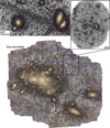 |
Fig. 1. General view of the Giant Coma Stream and its location in the Coma Cluster. Bottom: Color composite HERON image in the g and r bands. The dark background is constructed with the sum image. Uper right: WHT image of the Giant Coma Stream in L luminance (dark background) on a color image using g and r bands from the DECaLS survey. Upper left: Zoom onto the central region of the WHT image. |
2.2. WHT data
To obtain confirmation of this feature, we carried out follow-up observations with the 4.2 m William Herschel Telescope. We used the PF-QHY Camera with a field of view of 7.1′×10.7′ and pixel scale of 0.2667 arcsec pix−1. We used an L luminance filter, which is a UV-IR blocker with a high efficiency of 95% in the range of 370−720 nm, thus covering the g and r SDSS filters. The purpose of using a wide luminance band is to achieve maximum detection power given the extremely low surface brightness of this feature. A total of 200 individual 180 s exposures were obtained on June 4, 6, 11, and 14, 2021, under seeing conditions of approximately 1.2 arcsec. The data processing was similar to that used for the HERON data. Throughout the observations, we carried out extensive dithering, with maximum separation of about 5 arcmin (half of the field of view) in order to obtain high efficiency in the low-surface-brightness regime, minimizing the presence of gradients and allowing us to build a flat field with the science images.
Due to the extensive dithering of the observations, the exposure time varies with position. In Fig. A.1 we show the exposure time and equivalent depth along the footprint of the observations. In the maximum exposure region of 10 h, the limiting surface brightness reaches 31.4 mag arcsec−2 [3σ, 10″ × 10″] in the L luminance band. A relatively large portion of about 6 × 8 arcmin of the area of the image, including the central region of the stream, has a surface brightness limit of 31.0 mag arcsec−2 [3σ, 10″ × 10″]. The resolution is 1.2 arcsec in full width at half maximum (FWHM).
The WHT luminance band image confirms the existence of the narrow feature identified in the HERON data, achieving deeper surface brightness limits and higher resolution (see Figs. 1b and c) over the central region (14 × 17 arcmin) of the stream. We searched visually for potential remnants or overdensity from a parent galaxy. However, the stream appears completely featureless, especially in the higher resolution and deeper WHT image that samples the central region.
3. Association with the Coma Cluster
The detection of this stream in three images with two different telescopes allows us to confirm its discovery and to rule out a possible residual flux due to instrumentation or data processing.
The presence of globular clusters usually traces the trajectories of streams (Mackey et al. 2019), and can also provide an estimate of their distance through measurement of the peak of the globular cluster luminosity function (Rejkuba 2012). However, the HERON data do not have enough point-source depth, and do not allow color filtering with only the g and r bands. There are no HST data available over the area, and the only multi-band data available from DECaLS have insufficient point source depth, making detection of globular clusters infeasible until better data are obtained. In this section, we present an analysis performed to ensure that the detected feature is indeed a stellar stream located in Coma.
3.1. Potential resolved stars
We explore the possibility of the existence of an overdensity of point-like sources over the stream region, which would indicate a close distance. For this, we use SExtractor (Bertin 2006) with a detection threshold of 1σ. We do not apply any magnitude criteria other than selecting sources compatible with point-like sources, and for this we select sources with a stellarity index of higher than 0.5.
The middle panel of Fig. 2 shows the density of point-like sources that we can associate with low-luminosity stars. Interestingly, this stream is not resolved into stars in the WHT data, appearing as an extremely smooth and low-surface-brightness feature. Considering that this feature is not resolved into stars, we follow the analysis by Zackrisson et al. (2012) to impose a lower limit on distance. The fact that stars are unresolved in our highest-resolution data with a seeing of 1.2 arcsec and a surface brightness of approximately 29 mag arcsec−2 (detailed in later sections) suggests that the feature must be at a distance of at least 1 Mpc.
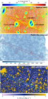 |
Fig. 2. Comparison between optical point-like source density and far-IR emission in the central region (13.5 × 7.6 arcmin). Top panel: WHT image in the luminance L filter color coded in surface brightness according to the upper color bar. Middle panel: density of detected point-like sources in the region with WHT data. Lower panel: 250 μm counterpart with the Herschel space telescope. The image is color coded in Sν according to the lower color bar. The dashed lines mark elliptical surface brightness contours of approximately μL = 26 mag arcsec−2 for the galaxies named in the top panel, and μL = 29.5 mag arcsec−2 for the location of the Giant Coma Stream. |
3.2. Far-infrared counterpart
In order to explore the possibility that the stream could be a trace of dust from the interstellar medium (ISM) or Galactic cirrus of the Milky Way, we used data available from the Herschel space telescope at 250 μm (Pilbratt et al. 2010). Due to its low temperature, Galactic cirrus are efficiently detected in far-infrared (FIR) and submillimeter bands (Low et al. 1984; Veneziani et al. 2010). The Herschel data at 250 μm offer a significant advantage over data from other instruments, such as IRAS (Neugebauer et al. 1984) or the Planck observatory with its 857 GHz band (Planck Collaboration XXIV 2011), both in detection power and – importantly for our case – resolution.
The lower panel of Fig. 2 shows a comparison between our optical data and the Herschel 250 μm band of the same field. The images have been stretched in the optical to provide maximum contrast for the detection of the faintest sources. The FWHM of the 250 μm Herschel data is 17.6 arcsec, which is lower than the detected stream width in optical bands of 1 arcmin. Visually, there is no emission trace in the 250 μm band, either in the region where the stream is located or adjacent to it. The only detectable emission in 250 μm is that corresponding to galaxies along the line of sight, among which we can highlight the strong emission from the late-type galaxy NGC 4848.
In order to quantify the 250 μm emission over the region of the stream, we calculated the total flux in the aperture defined by the dashed lines shown in Fig. 2 and outside this region. This aperture is defined using HERON optical data, and is detailed in Sect. 4.1. This is done on the heavily masked image, avoiding the integration of regions corresponding to external sources that appear in the image. The average sky background value over the region of the stream is Sν, 250 μm = −0.02 ± 0.04 MJy sr−1 and that outside this region is Sν, 250 μm = 0.02 ± 0.01 MJy sr−1. Therefore, the stream has no emission in the 250 μm band, at least up to the value defined by the sky background noise of these data.
The absence of a 250 μm counterpart to the optically detected stream suggests that the Galactic cirrus emission is an unlikely explanation for the origin of the feature. Additional reasons to rule out a Galactic cirrus contamination are that this celestial region is very close to the Galactic pole (b = 88°), with a low extinction by dust (Ar = 0.02 mag; Schlafly & Finkbeiner 2011) and that the stream is almost one dimensional, not showing the expected fractal morphology of cirrus in optical wavelengths (Marchuk et al. 2021).
3.3. Environmental analysis
The extremely low surface brightness of this feature makes it highly challenging to obtain spectroscopic information with which to measure its redshift. We have not found any gas detections in the region using the NASA/IPAC Extragalactic Database, nor counterparts in recent work by Bonafede et al. (2022).
Assuming that the feature is indeed a stellar stream, its elongated morphology suggests that it must be a tidal feature and therefore should be associated with some structure that impacts it gravitationally. Considering its large apparent size, beyond the obvious possible association with the adjacent Coma cluster, we explored a potential association with some nearby structures in close projection.
Figure 3 shows a celestial coordinate map with large-scale structures in the line of sight of the stream. We make use of the catalogue of nearby groups within 3500 km s−1 by Kourkchi & Tully (2017) to identify these structures. Kourkchi & Tully (2017) also offer estimates of the virial radius of these structures.
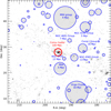 |
Fig. 3. Graphical representation of galactic associations in the line of sight of the Giant Coma Stream. Groups and clusters of local galaxies (Vrad < 3500 km s−1) and their apparent virial radii are represented with gray circles. Galaxies with redshift in the range of 3500 km s−1 < Vrad < 10 000 km s−1 are represented with black dots. The apparent Coma virial radius is represented with a red circle. The position and longitude of the Giant Coma Stream is represented with a red segment. |
We plot all groups together with their virial radii in Fig. 3. We convert from physical to projected coordinates using the same cosmological parameters as those in Kourkchi & Tully (2017) with H0 = 75 km s−1 Mpc−1. Where a distance is not available for a group, we use a direct conversion by Hubble’s law using the radial velocity. We find that only sparse groups do not have measured distances, and in any case, they are not close in projection to the Coma Cluster. As a complement, and given that the Kourkchi & Tully (2017) catalogue only contains groups up to 3500 km s−1, we plot galaxies with radial velocities of between 3500 and 10 000 km s−1 obtained from the NASA/IPAC Extragalactic Database as black points. This upper limit is used because it is the maximum radial velocity of the galaxies contained in the central region of the Coma cluster. To represent the virial radius of the Coma cluster, we rely on Ho et al. (2022), giving 2.4 Mpc with H0 = 75 km s−1 Mpc−1. We also plot the length and location of the stream as a red segment.
We can comment on some nearby structures. First, the Virgo Galaxy Cluster, which could be a potential host for the stream, is located at approximately 13° projected separation from Coma. With a calculated virial radius of 1.3 Mpc for the Virgo Cluster, this corresponds to an apparent size of 4.4°. The stream would therefore be located at a projected distance of 3.9 times the virial radius of the Virgo Cluster. The M 94 group is the other structure with a large apparent size, having a virial radius of 365 kpc, which is equivalent to 4.4°. The stream is located at three times the virial radius of the M 94 Group. NGC 4725, located at a distance of 12 Mpc, has a virial radius of 143 kpc, equivalent to 0.63°, with the stream at 5.1 times its virial radius. Next, the group of NGC 4565, located at a distance of 13 Mpc, has a virial radius of 343 kpc, equivalent to 1.4°, leaving the stream at more than 4.4 times its virial radius. Finally, the closest structure in terms of virial radius is M 64, located at a distance of 5 Mpc, with a virial radius of 224 kpc, equivalent to 2.34°. The stream would therefore be projected at a distance of 2.8 times this virial radius.
We explored the possibility that the stream could be caused by a disturbance from a galaxy that overlaps with it in the line of sight. In Fig. 2 the most prominent candidates are identified by name. In particular, the pair of overlapping galaxies UGC 08071 and LEDA 083688 could be candidates to produce the stream. However, our very deep images do not show any sign of asymmetry in them. Furthermore, the radial velocities of UGC 08071 and LEDA 083688 are 6933 ± 2 km s−1 and 8169 ± 2 km s−1, respectively, and these objects are therefore located more than 1200 km s−1 apart in velocity space (the radial velocity of galaxies in Coma ranges from 4000 to 10 000 km s−1). This makes it highly unlikely that they could have interacted at such a high velocity while leaving no asymmetry in the time during which the stream expanded. The other galaxies in the line of sight also show no appreciable asymmetry that would be compatible with the occurrence of the stream. We note that for a tidal-force calculation between galaxies in the line of sight, a distance value between them is necessary. However, in this case, a relative distance value is not easily obtained, considering that we are in a clustered environment, and that very close projections between galaxies might only be apparent. This would mean that galaxies in close projection could be separated by tens or even hundreds of kiloparsecs. We therefore consider the potential presence of disturbance in the outer parts of galaxy haloes to form the basis of the most reliable approach to identifying the presence of interaction between galaxies.
We further investigate a possible counterpart to a radio relic. Radio relics are diffuse structures detected in radio by synchrotron emission frequently found in interacting galaxy clusters (see a review by van Weeren et al. 2019). Notably, these radio relics are often found in the peripheral regions of galaxy clusters, with morphologies similar to those of the stream (Feretti et al. 2012; Jee et al. 2015). Although no optical counterpart has been found for these radio relics by previous works, due to the extreme surface brightnesses that we explore in this work, it is interesting to look for a counterpart to a radio relic. However, we do not identify a counterpart in the deepest and most recent data in Coma by Bonafede et al. (2022).
From this analysis, we conclude that the stream is embedded within the region of influence or virial radius of the Coma Galaxy Cluster, and does not overlap with the virial radius of any other structure in the line of sight. No other galactic association, such as a group or cluster, overlaps with the location of the stream, and there is no galaxy in the line of sight that could be the origin of the stream. This indicates that the stream is most likely associated with Coma and that there is no other particular galaxy or galactic association that can explain its clearly disturbed morphology.
4. Analysis
4.1. Photometry
To better constrain the nature and possible origin of the stream, we performed a photometric analysis of the Giant Coma Stream with the two different datasets available to us. The HERON image provides two photometric bands g and r with surface brightness limits of 29.5 mag arcsec−2 [3σ, 10″ × 10″] in g and r bands, respectively, in the region of interest, with a spatial resolution of ≈3 arcsec FWHM and completely covering the region. The WHT data partially cover the central region of the stream with an average depth of 31.0 mag arcsec−2 [3σ, 10″ × 10″] in the luminance band and a spatial resolution of approximately 1.2 arcsec in FWHM. Given the different characteristics of the two datasets, we performed a different analysis on each, focusing on obtaining different photometric properties.
We first analyzed the photometry using the HERON data. In the top panel of Fig. 4, we show a composite color image with both g and r bands from HERON. This image is useful for visualizing the full extent of the stream and its morphology. The apparent size in length and width of 18.5 × 1 arcmin by visual inspection corresponds to approximately 510 × 25 kpc at the Coma distance. The middle panels of Fig. 4 show the masking and subsequent binning (5 × 5 pixels, equivalent to 5.58 × 5.58 arcsec) of these data, allowing us to isolate the stream from external sources. We can see that the stream has a certain curvature. We estimate a radius of curvature of about 3620 arcsec, which is about 1°, and is equivalent to 1.7 Mpc. The Coma virial radius is 2.4 Mpc (Ho et al. 2022). In the middle panel of Fig. 4, we indicate with dashed lines the contours of an annular aperture of 45 arcsec in width with this calculated radius of curvature. This aperture is the width at which the stream is detected in the HERON data, corresponding approximately to a surface brightness of 30 mag arcsec−2 in the r band (the shallowest of the HERON data; see Sect. 2.1). This aperture is the same as the one used in Sect. 3.2 to explore the potential IR emission of the stream.
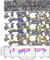 |
Fig. 4. Images and photometric profiles with HERON data. Top panel: composite color image with HERON in g and r bands. The high-contrast gray background is constructed with the sum g + r image. Middle panels: high-contrast images in the same field as the top panel in g, g + r, and r. Sources external to the stream were masked and the image was then rebinned to 5 × 5 pixels. The region bound by green dashed lines in the g + r image marks the position of the stream. Bottom panel: surface brightness profiles of the stream along the aperture indicated in the g + r image. HERON g and r bands are shown in blue and red, respectively, with an error of 1σ. Gray regions are spatial locations along the stream, which are discarded due to the absence of signal produced by the masking from external sources. |
We use this aperture on the masked image to derive g and r band photometric profiles along the stream, which are shown in the lower panel of Fig. 4. Because of the strong fluctuations in the profiles, we smooth them with a Gaussian kernel of approximately 10 binned pixel units in order to obtain a sufficient signal-to-noise ratio (S/N) in the profile. We calibrate the zero-flux sky level in the region adjacent to, but sufficiently far from, the stream. We find average surface brightnesses along the stream length of approximately 29.5 mag arcsec−2 in the g band and 29.0 mag arcsec−2 in the r band. The strong fluctuations of the photometric profiles of the stream are due to the extremely low surface brightness, together with the presence of masked regions, but also to possible systematic effects such as background fluctuation due to flat-fielding and sky subtraction.
Despite the obvious fluctuations, we observe that the difference between the g and r photometric profiles is relatively constant. Figure 5 shows the distribution of pixel color values for the stream. This latter faithfully follows a Gaussian function, compatible with a constant color that would correspond to the color of the stream. To obtain the average color and error, we calculate the mean value and error using a 3σ robust mean, yielding g − r = 0.53 ± 0.05 mag. This color indirectly indicates that a potential lensing of a high-redshift background source amplified by Coma can be ruled out, as a high-redshift source should appear much redder in g − r color, and additionally, Coma is too nearby to act effectively as a lens. In complement to this, we fit the distribution with a Gaussian function that provides an equivalent value (see Fig. 5). In order to obtain a pseudo color g − L with which to relate the photometric magnitudes between HERON (g and r bands) and WHT (L band), we constructed an image with the average of the g and r bands. Using this pseudo L band, we carried out a similar analysis, which yielded g − L = 0.32 ± 0.03 mag.
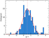 |
Fig. 5. Histogram of g − r color using HERON data at the selected aperture for the Giant Coma Stream (see Fig. 4). The solid red line shows the best fit to a Gaussian function. The dashed red vertical line marks the mean color calculated with a 3σ resistant mean. |
We now focus on the analysis of the WHT data, with higher nominal depth and better resolution, albeit only available in the central region of the stream. Figure 6 shows a photometric profile along the cross-section of the stream. The left panel shows a high-contrast image binned 5 × 5 from the original pixel size of 0.2667 arcsec, giving at a pixel scale of 1.334 arcsec. The central panel, shows this same image with masking applied to hide external sources to the stream. This masking is performed with a combination of SExtractor, which aggressively hides mainly sources of small sizes (DETECT_THRESH = 0.3), and a manual masking with wide circular apertures hiding larger galaxies and their expected haloes that could appear even below the surface brightness detectable visibly in the images. After this masking, the images are binned at 1.334 arcsec pix−1, allowing the diffuse light to emerge efficiently (see Román et al. 2021, for a similar processing).
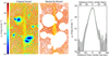 |
Fig. 6. Surface-brightness images and profiles with the WHT data in the luminance filter. Left panel: binned image at a size of 5 × 5 pixels (equivalent to 1.333 × 1.333 arcsec) color-coded in surface brightness and oriented so that the stream appears vertically. Middle panel: similar to left panel but with all external sources masked and then binned to 5 × 5 pixels. Right panel: photometric profile in the luminance band L (approximately equivalent to g + r) in the cross section (left-right) direction. The gray error regions correspond to 1σ. The widths in the transverse direction of the three panels coincide in spatial scale. |
Given the nearly straight morphology of the stream in this partial region, we project the combined flux in this direction, obtaining a photometric profile along the cross-section. This is done in the region of the image with a nominal depth of fainter than 31.0 mag arcsec−2 in the L band (see Fig. A.1), avoiding the outermost areas, which due to the dithering of the observations have a lower S/N. The whole region shown in the central panel is the one used for the photometric profile. For averaging, we use the median value along the stream direction, with errors calculated as 1σ. We introduce a tilt plane that fits the sky background in order to eliminate a small gradient present in the profile. The obtained profile is smoothed with a three-pixel Gaussian kernel to eliminate small fluctuations from the effects of masking.
The maximum surface brightness of the stream is approximately 29.2 mag arcsec−2 in the L band. Using the previously calculated g − L color of 0.32 mag, this would translate into a maximum surface brightness of approximately 29.5 mag arcsec−2 in the g band, agreeing with the values obtained from the HERON data, and giving confidence to the results. The WHT profile reaches reliably down to a surface brightness of about 32 mag arcsec−2, beyond which spurious fluctuations begin to show up, probably due to sky fluctuations and masking residuals. The shape of the profile is approximately straight in its slope, and is therefore compatible with an exponential decay. By analyzing this profile in flux units, we can identify an approximately Gaussian shape (see Fig. 7). By modeling this flux profile with a Gaussian function, the 1σ fitted width has a value of 20.1 arcsec or 9.3 kpc. The FWHM is 42.3 arcsec or 19.5 kpc. We notice a small asymmetry in the profile, where on the left side (toward the direction where Coma is located) the profile shows a slight excess. However, this asymmetry is not strong, and is potentially caused by the masking residuals of nearby galaxies located in that region.
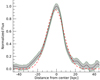 |
Fig. 7. Photometric profile equivalent to that in the right panel of Fig. 6 but in arbitrary flux units. The dashed red line indicates the best fit to a Gaussian function (see text). The gray error regions correspond to 1σ. |
Due to the numerous sources overlapping the stream, a direct flux measurement is not possible. In order to obtain an integrated magnitude, we use the good fit to a Gaussian profile to model the total flux. To this end, we assume the average profile to be that obtained in the analysis of Fig. 7 in order to integrate it along the estimated length of 510 kpc (see Fig. 4). We consider this a relatively good approximation because of the approximately constant surface brightness along the entire length of the stream. The value produced is L = 20.90 ± 0.12 mag, which corresponds to g = 21.22 ± 0.15 mag according to the color g − L = 0.32 ± 0.03 mag calculated above. The absolute magnitude of the stream according to this model at the distance of Coma would therefore be Lg = −13.78 ± 0.15 mag. Following mass to light ratio predictions by Roediger & Courteau (2015), this translates to a stellar mass of M⋆ = 6.8 ± 0.8 × 10⁷ M⊙. We note the potential presence of uncertainties on the integrated photometric quantities, both because of systematic errors due to modeling and possible nondetection of further structure in our data. Therefore, integrated magnitudes are to be considered as order-of-magnitude estimates, and as lower limits on the mass of both the stream and its potential progenitor.
According to the predicted mass–metallicity relations for a galaxy of this range of stellar mass (Panter et al. 2008; Simon 2019), a metallicity of approximately Z/H = −1 is expected. The color g − r = 0.53 ± 0.05 mag would therefore indicate that this is an old, passive dwarf galaxy according to single stellar population models by Vazdekis et al. (2015; see also Román & Trujillo 2017).
4.2. Similar structures in simulations
To obtain an idea of how such structures could arise in ΛCDM, we use the Illustris-TNG50 (TNG50 for short) simulations to insight the existence of similar streams in clusters. The TNG50 simulation has a box size ∼50 Mpc on a side and a baryonic mass-per-particle of ∼8.5 × 10⁴ M⊙. TNG50 is part of the Illustris-TNG suite of galaxy simulations in different volumes, which all include gravity, magnetohydrodynamics, and a treatment for the most relevant physical processes involved in galaxy formation, such as star formation, metal enrichment, and stellar and black hole feedback (Pillepich et al. 2018; Nelson et al. 2019).
It is difficult to estimate the frequency with which one should expect to observe the kind of thin structure seen for the Giant Coma Stream within the ΛCDM model. The formation of these thin structures will depend primarily on two circumstances: timing of the merger or infall, and the intrinsic properties of the progenitors. Tidal disruption that sets in too early with respect to the present time at z = 0 – at which we analyze the cluster – or progenitors that have overly extended intrinsic sizes will lead to stellar streams that are too wide to be comparable to the Giant Coma Stream. On the other hand, satellite infall that is too late or intrinsic sizes that are too compact will lead to insufficient disruption to generate stellar streams that are as long as this stream.
While the relatively small box size in TNG50 does not allow for clusters as massive as Coma to exist in the simulated volume, the high numerical resolution needed to resolve the inner properties of the progenitors with an estimated mass of M⋆ ∼ 108 − 9 M⊙ makes the 50 Mpc box the most adequate to conduct our analysis. From the TNG database, we use their friend-of-friends group information to identify spatially coherent groups (Davis et al. 1985), the information about haloes and subhaloes as provided by Subfind catalogs (Springel 2005; Dolag et al. 2009), and the SubLink merger trees (Rodriguez-Gomez et al. 2015).
The most massive cluster in TNG50 (group 0) has a virial mass of M200 ∼ 2 × 10¹⁴ M⊙ and a virial radius of r200 ∼ 1200 kpc (virial quantities are defined at the radius where the average enclosed density is 200 times the critical density of the Universe). We note that the mass of Coma is approximately larger by a factor of ten, M200 ∼ 2 × 10¹⁵ M⊙ (Ho et al. 2022), which means that that even analyzing the highest-mass cluster in TNG50 falls short of an appropriate comparison. Nevertheless, our use of the TNG50 simulation is justified given the mass and spatial resolution needed to explore the presence of such narrow streams with dwarf-mass progenitors as those inferred in our calculations.
In order to identify similar stream structures, we selected all dwarf galaxies in the stellar mass range of M⋆, max = 108 − 9 M⊙ that interacted with our group according to the SubLink merger trees; we refer to these as progenitors. The selection is done at the time of maximum stellar mass, M⋆, max. This gives us a total of 342 progenitors for group 0. We then focused our search on progenitors that have lost a significant fraction of their maximum stellar content, f⋆, bound < 45%, where the bound fraction refers to the fraction of stellar mass at z = 0 compared to the maximum stellar mass, because we are interested in progenitors of a sizable stellar stream. This cut is used as it is close to but smaller than half the maximum stellar mass of all satellites. In any case, the exact value of the cut has little impact on our results. For example, choosing all progenitors retaining 50% of their mass would only add two objects to the sample, which were identified to be accreted very late and to leave remnants at much larger distances than the observed structure. We therefore decided to keep our 45% mass cut as a good proxy for our progenitors.
In addition, to identify progenitors that created structures further out in the halo of the cluster, we require that the median radius (r50) of the stellar debris, here simply defined as the material that has been tidally removed according to our substructure finder Subfind, be larger than 800 kpc. Our final sample comprises 19 progenitors. The main panel in Fig. 8 shows an image created from the stellar debris of this sample.
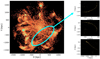 |
Fig. 8. Projected map of stellar remnants from the identified dwarf progenitors with M⋆, max = 108 − 9 M⊙ that fell into the most massive group simulated by the TNG50 simulation according to our selection criteria (see text). The map is color-coded by arbitrary surface brightness units, with a resolution of 30 arcsec. The most prominent candidate for a Coma stream analog is highlighted, and the right panels show 2D projected maps of only this remnant with a resolution of 1 arcsec (comparable to observational resolution). |
Encouragingly, within this sample, we find one particular stream with characteristics that are reminiscent of those of the Giant Coma Stream. The analogous structure is highlighted in cyan in the main panel of Fig. 8 and then shown in three perpendicular projections in the smaller panels on the right. Not only is this stream narrow and very extended as in the case of the Giant Coma Stream, but also under the right projection it appears as an almost straight line (when the projection is close to the orbital plane). We note that the center of curvature of the stream points toward the center of the cluster, as is the case for the Giant Coma Stream. This could be considered as further evidence that indeed the Giant Coma Stream belongs to Coma, because the approximate center of curvature coincides with the center of the gravitational potential about which they orbit (Nibauer et al. 2023).
Our simulated analog has a progenitor stellar mass of M⋆, max = 1.1 × 10⁸ and has lost ∼75% of its original mass at the present day, which is defined at snapshot 98 in the simulation, or redshift z = 0.009. Interestingly, the formation history of this stream is somewhat noncanonical, as the gravitational potential of the clusters is not the only environment responsible for the stellar stream formation. The tidal disruption leading to the formation of this thin stream seems to start as part of preprocessing in a smaller group environment. Our analog is first accreted into another group with a virial mass of M200 = 5.48 × 10¹¹ M⊙ at infall time tinf = 2.98 Gyr (zinf = 2.2, defined as the last time this dwarf galaxy was centered in its own dark matter halo). Only at later times, by t = 6.5 Gyr, does the analog join the friends-of-friends group of the main cluster, only crossing its virial radius by t ∼ 12.7 Gyr, making it a relatively recent accretion. At the final time, the analog has gone through only one pericenter around the main cluster, from which it recently emerged and is on its way to the first apocenter. The center of the group where the preprocessing occurred is currently more than 1000 kpc away from our analog.
The numerical resolution of TNG50 is insufficient to study the morphology of the stream in detail, for example, in terms of width or the light profile across the stream, for which hundreds of thousands of stellar particles would be needed to faithfully trace the structure (compared to the ∼10 000 available in TNG50 for this progenitor). Instead, this simulation provides a idea of a possible formation scenario for very narrow and long stellar streams in massive galaxy clusters, demonstrating that they do occur within the current cosmological scenario. Tailored idealized simulations would be the obvious next step to study and understand the detailed properties of the stream in terms of width, light profile, and color gradients.
5. Discussion
The properties of the Giant Coma Stream are remarkable. Its thin and coherent morphology is reminiscent of cold stellar streams observed in the Milky Way (e.g., Odenkirchen et al. 2003; Grillmair & Dionatos 2006; Balbinot et al. 2016) or streams in the Andromeda Galaxy (see a review by Ferguson & Mackey 2016). Its surface brightness peaks at a very faint level of 29.5 mag arcsec−2 in the g band (see Fig. 6), which is comparable to the surface brightness of the Giant Stream in the Andromeda Galaxy (Ibata et al. 2001). However, the size of the Giant Coma Stream, with a detected length of approximately 510 kpc, is longer than any known “giant” stream in the literature (Ibata et al. 2001; Martínez-Delgado et al. 2009, 2021, 2023b). To the best of our knowledge, no stellar stream of such size has ever been detected, nor has a stream of such low surface brightness been seen in surface photometry observations.
Previous work in Coma and other galaxy clusters revealed the presence of tidally disrupted objects (Trentham & Mobasher 1998; Gregg & West 1998; Conselice & Gallagher 1999; Calcáneo-Roldán et al. 2000) showing evidence for the build up of the intracluster light by accretion of substructures. We now discuss some particular cases. First, the plume-like object discovered by Gregg & West (1998) in the heart of Coma is 130 kpc long and about 15−30 kpc wide. Its surface brightness is much brighter (μR = 25.7 mag arcsec−2) than that of the Giant Coma Stream, as is its integrated luminosity (R = 15.6 ± 0.1 mag), and it is of a much redder color, namely g − r ≈ 0.75 mag (Gregg & West 1998). A simple calculation shows that the stellar mass of this plume-like object is approximately 1010 solar masses, indicating that the remnant is a much more massive galaxy than a dwarf, and is probably an elliptical galaxy, discarding a common origin. While the properties and locations of this plume-like object and the Giant Coma Stream differ, it is interesting that both share the same orientation, and that this orientation coincides in their alignment with the main filament that feeds Coma (see Malavasi et al. 2020). Additionally, correlated accretion due to the orientation of filaments and large-scale structure is expected to occur within ΛCDM (e.g., Libeskind et al. 2014). Another interesting object is the arc located in the Centaurus cluster discovered by Calcáneo-Roldán et al. (2000). Its morphology is remarkably similar to that of the Giant Coma Stream, with a linear and featureless appearance, and a length of ∼170 kpc (Calcáneo-Roldán et al. 2000). However, the surface brightness is considerably higher than that of the Giant Coma Stream with μR = 26.1 mag arcsec−2. Calcáneo-Roldán et al. (2000) argue that this object could be a tidally disrupted luminous spiral galaxy.
Several more recent studies have been carried out in a number of galaxy clusters (Giallongo et al. 2014; Montes & Trujillo 2018, 2022; DeMaio et al. 2018; Montes et al. 2021; Jiménez-Teja et al. 2021). The surface brightness and resolution (due to the close proximity of the Coma cluster) achieved in our work are unprecedented, with one exception. The Burrell Schmidt Deep Virgo Survey (Mihos et al. 2017) is comparable in terms of depth to our observations with the addition of a better resolution due to the proximity of the Virgo Cluster. Indeed, a large number of thin stellar streams appear in the central region of Virgo; for example, a pair of streams to the NW of M87 with lengths of around 150 kpc and similarly thin morphologies and widths of on the order of tens of kiloparsecs (streams A and B by Mihos et al. 2005; Rudick et al. 2010), as well as a myriad of much smaller streams or tidal features associated with different galaxies in the field of Virgo (Mihos et al. 2017).
A fundamental characteristic that differentiates the Giant Coma Stream from the streams detected in Virgo is that it is not associated with any particular galaxy but is a free-floating structure in the external regions of Coma. Dynamically cold and extremely faint stellar streams are thought to form through strong tidal fields in low-mass accretion events (Bullock & Johnston 2005), and in the case of galaxy clusters through interactions of low-mass galaxies passing through the inner region of the clusters (Romanowsky et al. 2012; Cooper et al. 2015). These streams are fragile, and dynamical times of one or two times the crossing time are enough to destroy them (Rudick et al. 2009). It is therefore striking that the Giant Coma Stream is a free-floating stream far from the center of the cluster, with such a coherent and fragile morphology.
We argue that the lack of detected free-floating streams in Virgo could be due to two factors. First, Coma is much more massive than Virgo, which implies a much higher velocity dispersion, σv = 1008 km s−1 for Coma (Struble & Rood 1999) versus σv = 638 km s−1 for Virgo (Kashibadze et al. 2020), and so high-velocity galaxies are more common in Coma. Second, a free-floating stream in Virgo would be expected to lie in the periphery of the cluster, but due to the proximity of Virgo, the deep data provided by Mihos et al. (2017) are limited to its central region. If a similar feature exists at a projected distance of the Giant Coma Stream, namely 0.8 Mpc, in Virgo, that stream would be outside the footprint of these observations and therefore undetected. This makes it potentially interesting to explore the outermost regions of the Virgo cluster or other nearby clusters in a search for similar free-floating streams analogous to the Giant Coma Stream.
The presence of an analog stream in the TNG-50 simulation may indicate that such free-floating streams with cold or thin morphology may be common in galaxy clusters. There is no guarantee that the Giant Coma Stream was formed by a complex interaction like the one depicted by our analog. However, it is encouraging that we find at least one analog in the formation history of a galaxy cluster. Our analysis indicates that while typical debris from this type of progenitor tends to be wider and less coherent than the Giant Coma Stream, at least there is one case where the narrowness and length of the stellar stream are comparable to it, suggesting that such structures may occur in ΛCDM. The recent accretion of this analog is compatible with the fragility of this type of structure, which, as mentioned above, is typically able to survive only one or two times the crossing time in its orbit by the cluster, making it very likely that the Giant Coma Stream is a recent accretion.
The potential presence of such thin stellar streams of cold morphology in galaxy clusters could extend the environmental range of their study from galactic to cluster scales. If cold stellar streams of considerably larger sizes than those found in the Local Group were found to be common, this would make current projections of their detectability much more optimistic (Pearson et al. 2019), and future observational work, including by Euclid, the Rubin Observatory, the Nancy Grace Roman Space Telescope or ARRAKIHS, will be necessary in order to unveil similar structures in galaxy clusters and the properties of both the Giant Coma Stream and potential new discoveries.
One of the imminent and most impactfull applications of the study of cold stellar streams is related to the possibility of testing the shapes of the dark matter haloes and the subhalo distribution in their hosts, as the presence and number of subhaloes is ultimately defined by the properties of dark matter particles (Ibata et al. 2002; Carlberg 2012; Erkal & Belokurov 2015). Ongoing work includes the analysis of the morphology and kinematics of cold stellar streams in the Milky Way, with the objective of tracing the global gravitational potential and also analyzing the possible impact of a low-mass dark matter subhalo that could perturb these streams both morphologically and kinematically (Erkal et al. 2016; Banik & Bovy 2019; Ibata et al. 2020; Banik et al. 2021).
The available observational data for the Giant Coma Stream are insufficient in both resolution and depth and therefore do not allow a detailed analysis of this stream. We recall that the maximum resolution of our data is approximately 1.2 arcsec FWHM, which is equivalent to 550 pc at the Coma distance. Additionally, radial velocity measurements of individual stars are fundamental to these analyses (Pearson et al. 2022). While current instrumental capabilities do not allow for such analyses, the new generation of extremely large-aperture telescopes may have sufficient observational capabilities for these studies.
6. Summary
In this work, we report the discovery of the Giant Coma Stream, a stellar stream with an extremely coherent and thin morphology, located at a distance of 0.8 Mpc from the center of the Coma cluster, and reminiscent of the cold stellar streams detected in the Milky Way.
-
The properties of the Giant Coma Stream are striking: a maximum surface brightness of μg = 29.5 mag arcsec−2 and a length of 510 kpc. This makes it the faintest stream ever detected by surface photometry. The stellar mass is estimated to be M⋆ = 6.8 ± 0.8 × 10⁷ M⊙ with a color of g − r = 0.53 ± 0.05 mag, which is consistent with a passive dwarf galaxy being the potential progenitor for the Giant Coma Stream. We do not identify any potential galaxy remnant or core, and the stream structure appears featureless in our data.
-
The Giant Coma Stream is orders of magnitude fainter in surface brightness than previous tidal features discovered in Coma and other clusters (Trentham & Mobasher 1998; Gregg & West 1998; Conselice & Gallagher 1999; Calcáneo-Roldán et al. 2000). It is comparable in surface brightness to the thin streams detected in Virgo (Mihos et al. 2017), however unlike these, the Giant Coma Stream does not appear to be associated with any particular galaxy, appearing as a free-floating feature in the outer regions of Coma.
-
Through analysis of the Illustris-TNG50 simulation, we find a remarkably similar analog, suggesting that such giant, extremely faint, and free-floating thin stellar streams may exist in galaxy clusters according to Λ-CDM.
This work shows a glimpse of the kind of structures waiting to be discovered in the ultralow-surface-brightness Universe. These structures, such as the Giant Coma Stream, show promising properties in revealing the ongoing hierarchical assembly of galaxy clusters and potentially unveiling the ultimate nature of dark matter.
Acknowledgments
We thank the two anonymous referees for a thorough review of our work. We thank Chris Mihos, Garreth William Martin and Claudio Dalla Vecchia for interesting discussions about the result. We acknowledge financial support from the State Research Agency (AEI-MCINN) of the Spanish Ministry of Science and Innovation under the grant “The structure and evolution of galaxies and their central regions” with reference PID2019-105602GB-I00/10.13039/501100011033, from the ACIISI, Consejería de Economía, Conocimiento y Empleo del Gobierno de Canarias and the European Regional Development Fund (ERDF) under grant with reference PROID2021010044, and from IAC project P/300724, financed by the Ministry of Science and Innovation, through the State Budget and by the Canary Islands Department of Economy, Knowledge and Employment, through the Regional Budget of the Autonomous Community. J.R. acknowledges funding from University of La Laguna through the Margarita Salas Program from the Spanish Ministry of Universities ref. UNI/551/2021-May 26, and under the EU Next Generation. R.M.R. acknowledges financial support from his late father Jay Baum Rich. I.T. and G.G. acknowledge support from the ACIISI, Consejería de Economía, Conocimiento y Empleo del Gobierno de Canarias and the European Regional Development Fund (ERDF) under grant with reference PROID2021010044 and from the State Research Agency (AEI-MCINN) of the Spanish Ministry of Science and Innovation under the grant PID2019-107427GB-C32 and IAC project P/302300, financed by the Ministry of Science and Innovation, through the State Budget and by the Canary Islands Department of Economy, Knowledge and Employment, through the Regional Budget of the Autonomous Community. The operation of the Jeanne Rich Telescope was assisted by David Gedalia and Osmin Caceres and is hosted by the Polaris Observatory Association. This work is based on service observations made with the William Herschel Telescope (programme SW2021a15) operated on the island of La Palma by the Isaac Newton Group of Telescopes in the Spanish Observatorio del Roque de los Muchachos of the Instituto de Astrofísica de Canarias.
References
- Akeson, R., Armus, L., Bachelet, E., et al. 2019, arXiv e-prints [arXiv:1902.05569] [Google Scholar]
- Balbinot, E., Yanny, B., Li, T. S., et al. 2016, ApJ, 820, 58 [CrossRef] [Google Scholar]
- Banik, N., & Bovy, J. 2019, MNRAS, 484, 2009 [NASA ADS] [CrossRef] [Google Scholar]
- Banik, N., Bovy, J., Bertone, G., et al. 2021, JCAP, 2021, 043 [Google Scholar]
- Belokurov, V., Zucker, D. B., Evans, N. W., et al. 2006, ApJ, 642, L137 [Google Scholar]
- Bertin, E. 2006, ASP Conf. Ser., 351, 112 [NASA ADS] [Google Scholar]
- Bertin, E., Mellier, Y., Radovich, M., et al. 2002, ASP Conf. Proc., 281, 228 [NASA ADS] [Google Scholar]
- Biviano, A. 1998, Untangling Coma Berenices: A New Vision of an Old Cluster, 1 [Google Scholar]
- Bonaca, A., & Hogg, D. W. 2018, ApJ, 867, 101 [NASA ADS] [CrossRef] [Google Scholar]
- Bonafede, A., Brunetti, G., Rudnick, L., et al. 2022, ApJ, 933, 218 [NASA ADS] [CrossRef] [Google Scholar]
- Bullock, J. S., & Johnston, K. V. 2005, ApJ, 635, 931 [Google Scholar]
- Calcáneo-Roldán, C., Moore, B., Bland-Hawthorn, J., et al. 2000, MNRAS, 314, 324 [CrossRef] [Google Scholar]
- Carlberg, R. G. 2012, ApJ, 748, 20 [Google Scholar]
- Conselice, C. J., & Gallagher, J. S. 1999, AJ, 117, 75 [NASA ADS] [CrossRef] [Google Scholar]
- Cooper, A. P., Cole, S., Frenk, C. S., et al. 2010, MNRAS, 406, 744 [Google Scholar]
- Cooper, A. P., Gao, L., Guo, Q., et al. 2015, MNRAS, 451, 2703 [Google Scholar]
- Crnojević, D., Sand, D. J., Spekkens, K., et al. 2016, ApJ, 823, 19 [Google Scholar]
- Davis, M., Efstathiou, G., Frenk, C. S., et al. 1985, ApJ, 292, 371 [NASA ADS] [CrossRef] [Google Scholar]
- DeMaio, T., Gonzalez, A. H., Zabludoff, A., et al. 2015, MNRAS, 448, 1162 [NASA ADS] [CrossRef] [Google Scholar]
- DeMaio, T., Gonzalez, A. H., Zabludoff, A., et al. 2018, MNRAS, 474, 3009 [Google Scholar]
- Dey, A., Schlegel, D. J., Lang, D., et al. 2019, AJ, 157, 168 [Google Scholar]
- Dolag, K., Borgani, S., Murante, G., et al. 2009, MNRAS, 399, 497 [NASA ADS] [CrossRef] [Google Scholar]
- Dodd, E., Callingham, T. M., Helmi, A., et al. 2023, A&A, 670, L2 [NASA ADS] [CrossRef] [EDP Sciences] [Google Scholar]
- Dubinski, J., Mihos, J. C., & Hernquist, L. 1999, ApJ, 526, 607 [CrossRef] [Google Scholar]
- Duc, P.-A., Cuillandre, J.-C., Karabal, E., et al. 2015, MNRAS, 446, 120 [Google Scholar]
- Erkal, D., & Belokurov, V. 2015, MNRAS, 454, 3542 [NASA ADS] [CrossRef] [Google Scholar]
- Erkal, D., Belokurov, V., Bovy, J., et al. 2016, MNRAS, 463, 102 [NASA ADS] [CrossRef] [Google Scholar]
- Euclid Collaboration (Scaramella, R., et al.) 2022a, A&A, 662, A112 [NASA ADS] [CrossRef] [EDP Sciences] [Google Scholar]
- Euclid Collaboration (Borlaff, A. S., et al.) 2022b, A&A, 657, A92 [NASA ADS] [CrossRef] [EDP Sciences] [Google Scholar]
- Feretti, L., Giovannini, G., Govoni, F., et al. 2012, A&ARv, 20, 54 [NASA ADS] [CrossRef] [Google Scholar]
- Ferguson, A. M. N., & Mackey, A. D. 2016, Tidal Streams in the Local Group and Beyond (Cham: Springer) [Google Scholar]
- Genina, A., Deason, A. J., & Frenk, C. S. 2023, MNRAS, 520, 3767 [NASA ADS] [CrossRef] [Google Scholar]
- Giallongo, E., Menci, N., Grazian, A., et al. 2014, ApJ, 781, 24 [Google Scholar]
- Gregg, M. D., & West, M. J. 1998, Nature, 396, 549 [NASA ADS] [CrossRef] [Google Scholar]
- Grillmair, C. J., & Dionatos, O. 2006, ApJ, 643, L17 [Google Scholar]
- Gu, M., Conroy, C., Law, D., et al. 2020, ApJ, 894, 32 [NASA ADS] [CrossRef] [Google Scholar]
- Helmi, A. 2020, ARA&A, 58, 205 [Google Scholar]
- Ho, M., Ntampaka, M., Rau, M. M., et al. 2022, Nat. Astron., 6, 936 [NASA ADS] [CrossRef] [Google Scholar]
- Ibata, R., Irwin, M., Lewis, G., et al. 2001, Nature, 412, 49 [NASA ADS] [CrossRef] [Google Scholar]
- Ibata, R. A., Lewis, G. F., Irwin, M. J., et al. 2002, MNRAS, 332, 915 [CrossRef] [Google Scholar]
- Ibata, R., Thomas, G., Famaey, B., et al. 2020, ApJ, 891, 161 [Google Scholar]
- Ibata, R., Malhan, K., Martin, N., et al. 2021, ApJ, 914, 123 [NASA ADS] [CrossRef] [Google Scholar]
- Ivezić, Ž., Kahn, S. M., Tyson, J. A., et al. 2019, ApJ, 873, 111 [Google Scholar]
- Jee, M. J., Stroe, A., Dawson, W., et al. 2015, ApJ, 802, 46 [NASA ADS] [CrossRef] [Google Scholar]
- Jiménez-Teja, Y., Dupke, R. A., Lopes de Oliveira, R., et al. 2019, A&A, 622, A183 [Google Scholar]
- Jiménez-Teja, Y., Vílchez, J. M., Dupke, R. A., et al. 2021, ApJ, 922, 268 [CrossRef] [Google Scholar]
- Johnston, K. V., Zhao, H., Spergel, D. N., et al. 1999, ApJ, 512, L109 [NASA ADS] [CrossRef] [Google Scholar]
- Johnston, K. V., Bullock, J. S., Sharma, S., et al. 2008, ApJ, 689, 936 [Google Scholar]
- Kashibadze, O. G., Karachentsev, I. D., & Karachentseva, V. E. 2020, A&A, 635, A135 [NASA ADS] [CrossRef] [EDP Sciences] [Google Scholar]
- Kelvin, L. S., Hasan, I., & Tyson, J. A. 2023, MNRAS, 520, 2484 [NASA ADS] [CrossRef] [Google Scholar]
- Knapen, J. H., & Trujillo, I. 2017, Astrophys. Space Sci. Lib., 434, 255 [NASA ADS] [CrossRef] [Google Scholar]
- Kourkchi, E., & Tully, R. B. 2017, ApJ, 843, 16 [NASA ADS] [CrossRef] [Google Scholar]
- Lang, D., Hogg, D. W., Mierle, K., et al. 2010, AJ, 139, 1782 [NASA ADS] [CrossRef] [Google Scholar]
- Libeskind, N. I., Knebe, A., Hoffman, Y., et al. 2014, MNRAS, 443, 1274 [NASA ADS] [CrossRef] [Google Scholar]
- Liu, M. C., & Graham, J. R. 2001, ApJ, 557, L31 [NASA ADS] [CrossRef] [Google Scholar]
- Low, F. J., Beintema, D. A., Gautier, T. N., et al. 1984, ApJ, 278, L19 [NASA ADS] [CrossRef] [Google Scholar]
- Mackey, D., Lewis, G. F., Brewer, B. J., et al. 2019, Nature, 574, 69 [NASA ADS] [CrossRef] [Google Scholar]
- Malavasi, N., Aghanim, N., Tanimura, H., et al. 2020, A&A, 634, A30 [NASA ADS] [CrossRef] [EDP Sciences] [Google Scholar]
- Marchuk, A. A., Smirnov, A. A., Mosenkov, A. V., et al. 2021, MNRAS, 508, 5825 [NASA ADS] [CrossRef] [Google Scholar]
- Martin, G., Bazkiaei, A. E., Spavone, M., et al. 2022, MNRAS, 513, 1459 [NASA ADS] [CrossRef] [Google Scholar]
- Martínez-Delgado, D., Pohlen, M., Gabany, R. J., et al. 2009, ApJ, 692, 955 [CrossRef] [Google Scholar]
- Martínez-Delgado, D., Gabany, R. J., Crawford, K., et al. 2010, AJ, 140, 962 [Google Scholar]
- Martínez-Delgado, D., Román, J., Erkal, D., et al. 2021, MNRAS, 506, 5030 [CrossRef] [Google Scholar]
- Martínez-Delgado, D., Cooper, A. P., Román, J., et al. 2023a, A&A, 671, A141 [NASA ADS] [CrossRef] [EDP Sciences] [Google Scholar]
- Martínez-Delgado, D., Roca-Fàbrega, S., Miró-Carretero, J., et al. 2023b, A&A, 669, A103 [NASA ADS] [CrossRef] [EDP Sciences] [Google Scholar]
- McConnachie, A. W., Ibata, R., Martin, N., et al. 2018, ApJ, 868, 55 [Google Scholar]
- Mihos, J. C. 2019, arXiv e-prints [arXiv:1909.09456] [Google Scholar]
- Mihos, J. C., Harding, P., Feldmeier, J., et al. 2005, ApJ, 631, L41 [NASA ADS] [CrossRef] [Google Scholar]
- Mihos, J. C., Harding, P., Feldmeier, J. J., et al. 2017, ApJ, 834, 16 [Google Scholar]
- Monachesi, A., Gómez, F. A., Grand, R. J. J., et al. 2019, MNRAS, 485, 2589 [NASA ADS] [CrossRef] [Google Scholar]
- Montes, M. 2022, Nat. Astron., 6, 308 [NASA ADS] [CrossRef] [Google Scholar]
- Montes, M., & Trujillo, I. 2018, MNRAS, 474, 917 [Google Scholar]
- Montes, M., & Trujillo, I. 2022, ApJ, 940, L51 [NASA ADS] [CrossRef] [Google Scholar]
- Montes, M., Brough, S., Owers, M. S., et al. 2021, ApJ, 910, 45 [CrossRef] [Google Scholar]
- Mouhcine, M., Ibata, R., & Rejkuba, M. 2010, ApJ, 714, L12 [NASA ADS] [CrossRef] [Google Scholar]
- Nelson, D., Springel, V., Pillepich, A., et al. 2019, Comput. Astrophys. Cosmol., 6, 2 [Google Scholar]
- Neugebauer, G., Habing, H. J., van Duinen, R., et al. 1984, ApJ, 278, L1 [NASA ADS] [CrossRef] [Google Scholar]
- Nibauer, J., Bonaca, A., & Johnston, K. V. 2023, ApJ, 954, 195 [NASA ADS] [CrossRef] [Google Scholar]
- Odenkirchen, M., Grebel, E. K., Dehnen, W., et al. 2003, AJ, 126, 2385 [Google Scholar]
- Panter, B., Jimenez, R., Heavens, A. F., et al. 2008, MNRAS, 391, 1117 [NASA ADS] [CrossRef] [Google Scholar]
- Pearson, S., Starkenburg, T. K., Johnston, K. V., et al. 2019, ApJ, 883, 87 [NASA ADS] [CrossRef] [Google Scholar]
- Pearson, S., Price-Whelan, A. M., Hogg, D. W., et al. 2022, ApJ, 941, 19 [NASA ADS] [CrossRef] [Google Scholar]
- Pilbratt, G. L., Riedinger, J. R., Passvogel, T., et al. 2010, A&A, 518, L1 [NASA ADS] [CrossRef] [EDP Sciences] [Google Scholar]
- Pillepich, A., Vogelsberger, M., Deason, A., et al. 2014, MNRAS, 444, 237 [Google Scholar]
- Pillepich, A., Nelson, D., Hernquist, L., et al. 2018, MNRAS, 475, 648 [Google Scholar]
- Planck Collaboration XXIV. 2011, A&A, 536, A24 [NASA ADS] [CrossRef] [EDP Sciences] [Google Scholar]
- Planck Collaboration VI. 2020, A&A, 641, A6 [NASA ADS] [CrossRef] [EDP Sciences] [Google Scholar]
- Reino, S., Rossi, E. M., Sanderson, R. E., et al. 2021, MNRAS, 502, 4170 [NASA ADS] [CrossRef] [Google Scholar]
- Rejkuba, M. 2012, Ap&SS, 341, 195 [Google Scholar]
- Rey, M. P., & Starkenburg, T. K. 2022, MNRAS, 510, 4208 [NASA ADS] [CrossRef] [Google Scholar]
- Rodriguez-Gomez, V., Genel, S., Vogelsberger, M., et al. 2015, MNRAS, 449, 49 [Google Scholar]
- Rich, R. M., Collins, M. L. M., Black, C. M., et al. 2012, Nature, 482, 192 [NASA ADS] [CrossRef] [Google Scholar]
- Rich, R. M., Brosch, N., Bullock, J., et al. 2017, IAU Symp., 321, 186 [Google Scholar]
- Rich, R. M., Mosenkov, A., Lee-Saunders, H., et al. 2019, MNRAS, 490, 1539 [Google Scholar]
- Roediger, J. C., & Courteau, S. 2015, MNRAS, 452, 3209 [NASA ADS] [CrossRef] [Google Scholar]
- Román, J., & Trujillo, I. 2017, MNRAS, 468, 4039 [Google Scholar]
- Román, J., Trujillo, I., & Montes, M. 2020, A&A, 644, A42 [NASA ADS] [CrossRef] [EDP Sciences] [Google Scholar]
- Román, J., Castilla, A., & Pascual-Granado, J. 2021, A&A, 656, A44 [NASA ADS] [CrossRef] [EDP Sciences] [Google Scholar]
- Romanowsky, A. J., Strader, J., Brodie, J. P., et al. 2012, ApJ, 748, 29 [Google Scholar]
- Rudick, C. S., Mihos, J. C., Frey, L. H., et al. 2009, ApJ, 699, 1518 [NASA ADS] [CrossRef] [Google Scholar]
- Rudick, C. S., Mihos, J. C., Harding, P., et al. 2010, ApJ, 720, 569 [Google Scholar]
- Sanders, J. L., & Binney, J. 2013, MNRAS, 433, 1826 [CrossRef] [Google Scholar]
- Schlafly, E. F., & Finkbeiner, D. P. 2011, ApJ, 737, 103 [Google Scholar]
- Simon, J. D. 2019, ARA&A, 57, 375 [NASA ADS] [CrossRef] [Google Scholar]
- Smirnov, A. A., Savchenko, S. S., Poliakov, D. M., et al. 2023, MNRAS, 519, 4735 [NASA ADS] [CrossRef] [Google Scholar]
- Springel, V. 2005, MNRAS, 364, 1105 [Google Scholar]
- Struble, M. F., & Rood, H. J. 1999, ApJS, 125, 35 [Google Scholar]
- Tal, T., van Dokkum, P. G., Nelan, J., et al. 2009, AJ, 138, 1417 [NASA ADS] [CrossRef] [Google Scholar]
- Trentham, N., & Mobasher, B. 1998, MNRAS, 293, 53 [NASA ADS] [CrossRef] [Google Scholar]
- Trujillo, I., D’Onofrio, M., Zaritsky, D., et al. 2021, A&A, 654, A40 [NASA ADS] [CrossRef] [EDP Sciences] [Google Scholar]
- van Weeren, R. J., de Gasperin, F., Akamatsu, H., et al. 2019, Space Sci. Rev., 215, 16 [Google Scholar]
- Vazdekis, A., Coelho, P., Cassisi, S., et al. 2015, MNRAS, 449, 1177 [Google Scholar]
- Veneziani, M., Ade, P. A. R., Bock, J. J., et al. 2010, ApJ, 713, 959 [Google Scholar]
- Zackrisson, E., de Jong, R. S., & Micheva, G. 2012, MNRAS, 421, 190 [NASA ADS] [Google Scholar]
- Zwicky, F. 1933, Helv. Phys. Acta, 6, 110 [NASA ADS] [Google Scholar]
- Zwicky, F. 1951, PASP, 63, 61 [NASA ADS] [CrossRef] [Google Scholar]
Appendix A: Exposure times and depth in the WHT data
The left panel of Fig. A.1 shows the exposure time footprint for the WHT data. In order to provide a map of surface brightness limits, we performed the correlation between the standard deviation for pixels with equal exposure time and the exposure time. This correlation is shown graphically in Fig. A.2. The parameters of the best fit are
![Mathematical equation: $$ \begin{aligned} \mu _{lim,L} = -2.55\times log\left(\frac{1}{\sqrt{t_{exp}[h]}}\right)+30.13\;mag\;arcsec^{-2}, \end{aligned} $$](/articles/aa/full_html/2023/11/aa46780-23/aa46780-23-eq1.gif)
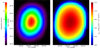 |
Fig. A.1. Maps of exposure time (left panel) and equivalent limiting surface brightness (right panel) for the WHT data in the luminance band (equivalent to g + r SDSS filters). Images cover a 14.15 x 17.67 arcmin rectangle. North is up, east to the left. |
 |
Fig. A.2. Linear correlation between exposure time and surface brightness limits measured as 3σ in 10×10 arcsec boxes for the WHT data. The blue line marks the correlation data obtained. The black dashed line marks the best fit of the correlation (see text). |
measured as 3σ in 10×10 arcsec boxes. By means of this obtained relation, we can make a surface brightness map using the exposure time values for each pixel. This map is shown in the right panel of Fig. A.1.
All Figures
|
Fig. 1. General view of the Giant Coma Stream and its location in the Coma Cluster. Bottom: Color composite HERON image in the g and r bands. The dark background is constructed with the sum image. Uper right: WHT image of the Giant Coma Stream in L luminance (dark background) on a color image using g and r bands from the DECaLS survey. Upper left: Zoom onto the central region of the WHT image. |
| In the text | |
|
Fig. 2. Comparison between optical point-like source density and far-IR emission in the central region (13.5 × 7.6 arcmin). Top panel: WHT image in the luminance L filter color coded in surface brightness according to the upper color bar. Middle panel: density of detected point-like sources in the region with WHT data. Lower panel: 250 μm counterpart with the Herschel space telescope. The image is color coded in Sν according to the lower color bar. The dashed lines mark elliptical surface brightness contours of approximately μL = 26 mag arcsec−2 for the galaxies named in the top panel, and μL = 29.5 mag arcsec−2 for the location of the Giant Coma Stream. |
| In the text | |
|
Fig. 3. Graphical representation of galactic associations in the line of sight of the Giant Coma Stream. Groups and clusters of local galaxies (Vrad < 3500 km s−1) and their apparent virial radii are represented with gray circles. Galaxies with redshift in the range of 3500 km s−1 < Vrad < 10 000 km s−1 are represented with black dots. The apparent Coma virial radius is represented with a red circle. The position and longitude of the Giant Coma Stream is represented with a red segment. |
| In the text | |
|
Fig. 4. Images and photometric profiles with HERON data. Top panel: composite color image with HERON in g and r bands. The high-contrast gray background is constructed with the sum g + r image. Middle panels: high-contrast images in the same field as the top panel in g, g + r, and r. Sources external to the stream were masked and the image was then rebinned to 5 × 5 pixels. The region bound by green dashed lines in the g + r image marks the position of the stream. Bottom panel: surface brightness profiles of the stream along the aperture indicated in the g + r image. HERON g and r bands are shown in blue and red, respectively, with an error of 1σ. Gray regions are spatial locations along the stream, which are discarded due to the absence of signal produced by the masking from external sources. |
| In the text | |
|
Fig. 5. Histogram of g − r color using HERON data at the selected aperture for the Giant Coma Stream (see Fig. 4). The solid red line shows the best fit to a Gaussian function. The dashed red vertical line marks the mean color calculated with a 3σ resistant mean. |
| In the text | |
|
Fig. 6. Surface-brightness images and profiles with the WHT data in the luminance filter. Left panel: binned image at a size of 5 × 5 pixels (equivalent to 1.333 × 1.333 arcsec) color-coded in surface brightness and oriented so that the stream appears vertically. Middle panel: similar to left panel but with all external sources masked and then binned to 5 × 5 pixels. Right panel: photometric profile in the luminance band L (approximately equivalent to g + r) in the cross section (left-right) direction. The gray error regions correspond to 1σ. The widths in the transverse direction of the three panels coincide in spatial scale. |
| In the text | |
|
Fig. 7. Photometric profile equivalent to that in the right panel of Fig. 6 but in arbitrary flux units. The dashed red line indicates the best fit to a Gaussian function (see text). The gray error regions correspond to 1σ. |
| In the text | |
|
Fig. 8. Projected map of stellar remnants from the identified dwarf progenitors with M⋆, max = 108 − 9 M⊙ that fell into the most massive group simulated by the TNG50 simulation according to our selection criteria (see text). The map is color-coded by arbitrary surface brightness units, with a resolution of 30 arcsec. The most prominent candidate for a Coma stream analog is highlighted, and the right panels show 2D projected maps of only this remnant with a resolution of 1 arcsec (comparable to observational resolution). |
| In the text | |
|
Fig. A.1. Maps of exposure time (left panel) and equivalent limiting surface brightness (right panel) for the WHT data in the luminance band (equivalent to g + r SDSS filters). Images cover a 14.15 x 17.67 arcmin rectangle. North is up, east to the left. |
| In the text | |
|
Fig. A.2. Linear correlation between exposure time and surface brightness limits measured as 3σ in 10×10 arcsec boxes for the WHT data. The blue line marks the correlation data obtained. The black dashed line marks the best fit of the correlation (see text). |
| In the text | |
Current usage metrics show cumulative count of Article Views (full-text article views including HTML views, PDF and ePub downloads, according to the available data) and Abstracts Views on Vision4Press platform.
Data correspond to usage on the plateform after 2015. The current usage metrics is available 48-96 hours after online publication and is updated daily on week days.
Initial download of the metrics may take a while.