| Issue |
A&A
Volume 679, November 2023
|
|
|---|---|---|
| Article Number | A55 | |
| Number of page(s) | 19 | |
| Section | Planets and planetary systems | |
| DOI | https://doi.org/10.1051/0004-6361/202244752 | |
| Published online | 07 November 2023 | |
The GAPS programme at TNG
XLVIII. The unusual formation history of V1298 Tau★
1
INAF – Osservatorio Astrofisico di Torino,
via Osservatorio 20,
10025
Pino Torinese, Italy
e-mail: This email address is being protected from spambots. You need JavaScript enabled to view it.
2
ICSC – National Research Centre for High Performance Computing, Big Data and Quantum Computing,
Via Magnanelli 2,
40033
Casalecchio di Reno, Italy
3
INAF – Istituto di Astrofisica e Planetologia Spaziali,
via Fosso del Cavaliere 100,
00133
Roma, Italy
4
Dipartimento di Fisica e Astronomia – Università di Padova,
Via Marzolo 8,
35121
Padova, Italy
5
INAF – Osservatorio Astronomico di Padova,
Vicolo dell’Osservatorio 5,
35122,
Padova, Italy
6
INAF – Osservatorio Astronomico di Trieste,
Via G. B. Tiepolo 11,
34143,
Trieste, Italy
7
INAF – Osservatorio Astronomico di Palermo,
Piazza del Parlamento, 1,
90134,
Palermo, Italy
8
Space Science Data Center - ASI,
Via del Politecnico snc,
00133
Roma, Italy
9
Instituto de Astrofísica de Canarias,
38200
La Laguna, Tenerife, Spain
10
Universidad de La Laguna, Dept. Astrofísica,
38206
La Laguna, Tenerife, Spain
11
INAF – Osservatorio Astronomico di Roma,
Via Frascati 33,
00040,
Monte Porzio Catone, Italy
12
School of Physical Sciences, The Open University,
Walton Hall,
Milton Keynes
MK7 6AA, UK
13
SUPA, Institute for Astronomy, University of Edinburgh,
Blackford Hill,
Edinburgh
EH9 3HJ, UK
14
INAF – Osservatorio Astronomico di Brera,
Via E. Bianchi 46,
23087,
Merate, Italy
15
Instituto Nacional de Astrofísica, Óptica y Electrónica,
Luis Enrique Erro 1,
Sta. Ma. Tonantzintla, Puebla, Mexico
16
Université Côte d’Azur, Observatoire de la Côte d’Azur, CNRS, Laboratoire Lagrange,
Nice, France
17
Université Grenoble Alpes, CNRS, IPAG,
38000
Grenoble, France
18
Geneva Observatory, University of Geneva,
Chemin Pegasi 51,
1290
Versoix, Switzerland
19
Department of Astronomy, Stockholm University, AlbaNova University Center,
10691
Stockholm, Sweden
20
CRAL, UMR 5574, CNRS, Université de Lyon,
Ecole Normale Supérieure de Lyon, 46 allée d’Italie,
69364
Lyon Cedex 07, France
21
INAF – Osservatorio Astrofisico di Catania,
Via Santa Sofia 78,
95123
Catania, Italy
22
Department of Physics and Astronomy, University of Exeter,
Stocker Road,
Exeter
EX4 4QL, UK
23
INAF – Osservatorio Astronomico di Cagliari,
Via della Scienza 5,
09047
Selargius, Italy
24
Department of Physics, University of Rome “Tor Vergata”,
Via della Ricerca Scientifica 1,
00133,
Roma, Italy
25
Max Planck Institute for Astronomy,
Königstuhl 17,
69117,
Heidelberg, Germany
26
Aix-Marseille Univ., CNRS, CNES, LAM,
Marseille, France
Received:
15
August
2022
Accepted:
4
July
2023
Abstract
Context. Observational data from space- and ground-based campaigns have revealed that the 10-30 Ma old V1298Tau star hosts a compact and massive system of four planets. Mass estimates are available for the two outer giant planets and point to unexpectedly high densities for their young ages.
Aims. We investigate the formation of these two outermost giant planets, V1298 Tau b and e, and the present dynamical state of V1298 Tau’s global architecture in order to shed light on the history of this young and peculiar extrasolar system.
Methods. We performed detailed N-body simulations to explore the link between the densities of V1298 Tau b and e and their migration and accretion of planetesimals within the native circumstellar disk. We combined N-body simulations and the normalized angular momentum deficit (NAMD) analysis of the architecture to characterize V1298 Tau’s dynamical state and connect it to the formation history of the system. We searched for outer planetary companions to constrain V1298 Tau’s planetary architecture and the extension of its primordial circumstellar disk.
Results. The high densities of V1298 Tau b and e suggest they formed at quite a distance from their host star, likely beyond the CO2 snowline. The higher nominal density of V1298 Tau e suggests it formed farther out than V1298 Tau b. The current architecture of V1298 Tau is not characterized by resonant chains. Planet-planet scattering with an outer giant planet is the most likely cause for the lack of a resonant chain between V1298 Tau’s planets, but currently our search for outer companions using SPHERE and Gaia observations can exclude only the presence of planets more massive than 2 MJ.
Conclusions. The most plausible scenario for V1298 Tau’s formation is that the system formed by convergent migration and resonant trapping of planets born in a compact and plausibly massive disk. In the wake of their migration, V1298 Tau b and e would have left a dynamically excited protoplanetary disk, naturally creating the conditions for the later breaking of the resonant chain by planet-planet scattering.
Key words: planetary systems / stars: individual: V1298 Tau / planets and satellites: formation / planets and satellites: dynamical evolution and stability / planets and satellites: detection / chaos
Based on observations made with the Italian Telescopio Nazionale Galileo (TNG) operated by the Fundaciòn Galileo Galilei (FGG) of the Istituto Nazionale di Astrofisica (INAF) at the Observatorio del Roque de los Muchachos (La Palma, Canary Islands, Spain).
© The Authors 2023
 Open Access article, published by EDP Sciences, under the terms of the Creative Commons Attribution License (https://creativecommons.org/licenses/by/4.0), which permits unrestricted use, distribution, and reproduction in any medium, provided the original work is properly cited.
This article is published in open access under the Subscribe to Open model. This email address is being protected from spambots. You need JavaScript enabled to view it. to support open access publication.
1 Introduction
Young planets offer us the unique opportunity to study unaltered products of planet formation, before secular evolution and interactions with host stars modify or cancel the original characteristics of the planets. When they belong to multiplanet systems, young planets also represent invaluable case studies to comparatively investigate how different formation histories can shape planets born from the same stellar and disk environments.
Multiple authors (e.g., Donati et al. 2016; Yu et al. 2017; Benatti et al. 2021) have argued that the population of massive planets in close orbits around young stars can be significantly larger than that of their counterparts around older stars. The proposed roots of this difference are the mass loss in the early evolutionary stages driven by the strong X and UV radiation from the host star, as well as the processes of orbital migration and chaotic evolution at play during the early phases of planetary systems that favor the engulfment (e.g., Donati et al. 2017; Spina et al. 2021) or the removal (e.g., Zinzi & Turrini 2017; Turrini et al. 2018, 2020, 2022) of planets.
Because young stars are usually very active, another reason for this difference could reside in the false positives induced by stellar activity. The number of known young planets has been questioned by recent works that have unveiled fake detections (e.g., Carleo et al. 2018; Donati et al. 2020; Damasso et al. 2020). In the past years, however, NASA Kepler and its K2 campaigns (Borucki et al. 2003; Howell et al. 2014) and recently the Transiting Exoplanet Survey Satellite (TESS; Ricker et al. 2015) detected transits of several young and multiple planets (e.g., David et al. 2016; Mann et al. 2016; Rizzuto et al. 2020; Plavchan et al. 2020), allowing the study of the early evolution and architecture of these systems (e.g., Benatti et al. 2019, 2021).
Analyzing the Kepler light curve of the young star Vl298 Tau (K2 Mission; Howell et al. 2014), David et al. (2019a) first discovered a Jupiter-sized planet (V1298 Tau b), and soon after David et al. (2019b) added three other planets following a forward analysis of the K2 Campaign 4 photometry. The transits of all four planets were later observed with TESS (Feinstein et al. 2022), confirming that V1298 Tau’s system is host to two Neptune-sized planets (dubbed “c” and “d”) and two Jovian-sized planets (“b” and “e”) – names are listed in order of distance from the parent star. The four planets inhabit an orbital region comparable to that contained within Mercury’s orbit in the Solar System.
In the framework of the Global Architecture of Planetary Systems project (GAPS; Covino et al. 2013; Carleo et al. 2020) and in collaboration with other groups, V1298 Tau was later observed by means of an intensive spectroscopic campaign. The GAPS campaign attained radial velocity (RV) measurements using several high-resolution spectrographs (HARPS-N, CARMENES, SES, and HERMES; Suárez Mascareño et al. 2022) in orderto constrain the masses of the fourplanets. These observations (Suárez Mascareño et al. 2022), combined with the constraints from Kepler and K2, yielded mass values for both planet b (0.64 ± 0.19 MJ) and planet e (1.16 ± 0.30 MJ), while they provided only upper limits for planets c and d (<0.24 and <0.31 MJ, respectively). Notwithstanding the uncertainties affecting the mass estimates, the GAPS survey has revealed that V1298 Tau is one of the most massive systems among those characterized by compact orbital architectures discovered so far.
Using the ExoplAn3T online tool (Exoplanet Analysis and 3D visualization Tool1; Zinzi et al. 2021a,b) developed by the Space Science Data Center of the Italian Space Agency, we queried the NASA Exoplanet Archive2 on the 8 May 2023 to search for massive exoplanetary systems with similarly compact architectures. We searched for systems with multiplicity greater than two around solar-type stars, orbital periods lower than 100 days, and at least one planet with a mass greater than 100 M⊕ being hosted. The only systems satisfying these constraints are V1298 Tau, Kepler-46 (three planets, two giants) and Kepler-256 (four planets, one giant). Adding the further requirement that the total planetary mass is greater than 1 MJ restricted this list to V1298 Tau and Kepler-46 only.
The availability of both planetary radii and masses for planets b and e allows for the estimation of their bulk densities. The values derived by Suárez Mascareño et al. (2022) using the planetary radii from Kepler and K2 are 1.2 ± 0.45 and 3.6 ± 1.6 g cm−3 for planets b and e, respectively. While affected by large uncertainties, these values are significantly greater than those predicted by formation theories for their age. Two possible explanations are discussed by Suárez Mascareño et al. (2022): the more rapid contraction of these young planets than predicted by interior evolution models or their extreme enrichment in heavy elements.
While the first possibility implies the need to revise our current understanding of giant planet evolution (Suárez Mascareño et al. 2022), the second explanation naturally arises from the planet formation process when giant planets undergo extensive migration within their native disk (Thorngren et al. 2016; Shibata et al. 2020; Turrini et al. 2021). The conclusions drawn by Suárez Mascareño et al. (2022) are also valid for the new measurements of the radii of V1298 Tau’s planets from the photometric observations by TESS (Feinstein et al. 2022), which update the densities of planets b and e upward and downward, respectively (roughly by about 30%).
The architecture of V1298 Tau’s planets initially appeared very close to being in a resonant chain. In particular, the orbit of the fourth planet was originally assessed by Suárez Mascareño et al. (2022) to be close to completing a resonant chain, either 3:2, 2:1, and 3:2 or 3:2, 2:1, and 2:1. However, the period ratio between planet b and d is too far from a 2:1 resonant ratio, effectively excluding the possibility that the system is currently in a resonant chain (Tejada Arevalo et al. 2022). Furthermore, recent data indicate an orbital period of planet e (Feinstein et al. 2022; Damasso et al. 2023) that is not in resonance with that of planet b.
The combination of the masses and densities of planets b and e and the compact architecture of V1298 Tau points toward the system having formed by convergent migration within the circumstellar disk followed by resonant trapping. The trapping in a stable resonant configuration is particularly important for planets b and e, as they would otherwise become unstable long before reaching their current compact orbits. In this scenario, however, the current non-resonant orbits of its planets require that the system underwent a phase of instability that broke the original resonant chain despite its young age (Tejada Arevalo et al. 2022).
In this work, we jointly study the formation of V1298 Tau’s planets b and e and their orbital architecture with the aim of shedding light on V1298 Tau’s unusual formation history. We complement our study with new observations of V1298 Tau, searching for additional outer planets to constrain the extension of the planet-forming region in V1298 Tau’s circumstellar disk. As we later show, the convergent and large-scale migration required to explain the high density values and compact orbits of V1298 Tau b and e naturally creates the conditions to evolve the planetary system into its present configuration.
This paper is organized as follows: in Sect. 2 we revise the fundamental parameters of V1298 Tau’s planets based on the most up-to-date observations, while in Sect. 3 we describe the numerical algorithms used in modeling their formation, their capture in resonance, and the onset of their subsequent instability. In Sect. 4, we outline our results concerning the history of the planetary system and the conditions that can lead to its present non-resonant configuration. Section 5 is devoted to observational constraints on the presence of additional planets in outer orbits obtained with SPHERE (the Spectro-Polarimetric High-contrast Exoplanet REsearch facility at the VLT telescope), while in Sect. 6 we discuss the implications of our results and combine them in a unified picture.
2 Vl298 Tau: The star and its planets
With its estimated age ranging between 10 and 30 Ma (Suárez Mascareño et al. 2022; Maggio et al. 2022), V1298 Tau is one of the youngest solar-type planet-host stars. As its Teff = 5050 ± 100 K, V1298 Tau is a K1 spectral type with iron abundance [Fe/H] = 0.10 ± 0.15 dex (Suárez Mascareño et al. 2022), and it belongs to the young stellar group 29 identified by Oh et al. (2017). The star is characterized by a high and steady activity level, causing large RV activity variations, as also testified by the value of < log(R′HK) > = −4.2397 ± 0.0179 determined by GAPS (Suárez Mascareño et al. 2022). We report the main stellar parameters of V1298 Tau in Table 1.
From XMM-Newton observations, Maggio et al. (2022) found that this young star has a bolometric luminosity ratio of logLX/log LBol =  , confirming that it is an X-ray bright young star near the saturated emission regime observed for G-K stars. Despite the close position of the four planets to their star (see Table 1), Maggio et al. (2022) found that the two outer planets (b and e) are not affected by evaporation on timescales of billions of years. The two inner planets (c and d) are also impervious to evaporation if their masses are higher than 40 M⊕.
The analysis performed by Suárez Mascareño et al. (2022) to derive the mass of planet e attributed an orbital period of 40 days to the planet. The subsequent observations by TESS led to this value being revised upward, suggesting a most probable period of 44 days and providing additional discreet solutions for larger orbital periods characterized by decreasing probabilities (Feinstein et al. 2022). The TESS observations also led to the planetary radii of planets b and e being revised downward and upward, respectively (Feinstein et al. 2022). Following these new observations, we reevaluated the mass of planet e and then updated its density as well as that of planet b.
To reassess the mass of planet e accounting for the larger possible values of its orbital period, we reanalyzed the RV dataset from Suárez Mascareño et al. (2022), imposing the additional constraint to the priors that the orbital period of planet e should not be smaller than 44 days. Feinstein et al. (2022) showed that an orbital period shorter than this value would result in an unobserved second transit within the TESS baseline. Previously, K2 data only constrained the orbital period to values higher than 36 days. Following the results of Feinstein et al. (2022), we used a half-normal distribution starting at 44 days, with a sigma of 7 days, as the prior for the period of planet e. Apart from this additional prior, our analysis is the same as described in Suárez Mascareño et al. (2022).
We fit K2 photometry, ground-based photometry, and RV time series simultaneously. We modeled the activity signals in all datasets using a Gaussian processes regression with celerite (Foreman-Mackey et al. 2017). The K2 photometry was used to obtain information on the parameters of the transits. The ground-based photometric data is contemporary to the RV data and helped constrain the parameters of the stellar activity model. To sample the posterior distribution, we relied on nested sampling (Skilling 2004) using dynesty (Speagle 2020). For more details and a full description of the priors used in the global model, we refer the reader to Suárez Mascareño et al. (2022).
The priors and posteriors of the analysis are shown in the top row of Fig. 1, while the bottom row shows the derived planetary and orbital parameters of planet e. The new mass value of planet e is  , which is slightly higher yet consistent within 1-σ with the previous value from Suárez Mascareño et al. (2022). Our analysis also updates the plausible periods of V1298 Tau e and shows that the most likely values are at 45 and 46 days, with two possible lower-probability solutions at 44 and 47.7 days (see Fig. 1). While multimodal posteriors, like those characterizing the orbital period, are known to be difficult to sample with traditional MCMC methods, nested sampling methods in general, and dynesty in particular, have been shown to be able to sample them robustly and efficiently (Speagle 2020).
None of the solutions presented above results in a resonant coupling between planets b and e. Preliminary results from ongoing observations of the ESA mission CHEOPS exclude the solutions at 44 and 46 days and are instead compatible with the one at about 45 days (Damasso et al. 2023), which we adopted as the nominal period of V1298 Tau e in this work.
The full updated characterization of V1298 Tau’s four planets is reported in Table 1. Figure 1 and Table 1 show that, like its mass, the eccentricity of planet e is higher than that estimated by Suárez Mascareño et al. (2022), but also in this case, the two values are consistent at the 1-σ level.
Main stellar and planetary parameters of V1298 Tau’s system.
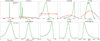 |
Fig. 1 New analysis of the RV dataset and its results on planet e. Top: priors and posteriors of the new analysis from Suárez Mascareño et al. (2022) where we include the constraints from TESS on its orbital period (Feinstein et al. 2022). Bottom: derived distributions of the planetary and orbital parameters. We note that we used the updated planetary radius from TESS (Feinstein et al. 2022) in our analysis in place of the one appearing in this figure, which is still based on the Kepler and K2 data, as in Suárez Mascareño et al. (2022). |
2.1 Dynamical excitation of V1298 Tau b and e
We used the updated architecture of V1298 Tau from Table 1 to investigate the dynamical excitation of planets b and e by means of their normalized angular momentum deficit (NAMD; see Chambers 2001; Turrini et al. 2020). The NAMD provides an architecture-agnostic measure of dynamical excitation that can intuitively be interpreted as the “dynamical temperature” of planetary systems. Stated simply, the higher the value, the more excited the dynamical state of the system. We adopted the NAMD of the Solar System (1.3 × 10⁻³; Turrini et al. 2020) as the boundary between dynamically cold and hot orbits (see Carleo et al. 2021; Turrini et al. 2022 for a discussion).
Following Carleo et al. (2021), the goal of our analysis is not to pinpoint the exact value of V1298 Tau’s NAMD but to verify if, notwithstanding the uncertainties on the physical and orbital parameters of its planets, its dynamical excitation is systematically higher than that of the Solar System and whether it indicates past or current phases of dynamical instability. We accounted for the uncertainties on the mass, semimajor axis, and eccentricity of the two planets following the Monte Carlo approach described in Turrini et al. (2020) and Carleo et al. (2021). To better sample the effects of the large uncertainties of these parameters on the NAMD, we used 106 extractions for each parameter in place of the original 104 proposed by Laskar & Petit (2017).
Based on the low mutual inclination of the two planets (<1º; see Table 1) that limitedly contributes to the NAMD, we assumed the two orbits to be coplanar. Due to the positive-defined nature of the NAMD, this choice means that we err toward lower excitations. The resulting NAMD modal value (2.2 × 10⁻²) is 17 times higher than that of the Solar System, with the 3σ range extending from five times (6.4 × 10⁻³) to 120 times (0.16) that of the Solar System. As discussed by Turrini et al. (2020, 2022) and illustrated by the recent study by Rickman et al. (2023), such a systematically high range of NAMD values is associated with phases of dynamical instability and planet-planet scattering events (either in the past or presently).
The results of the NAMD analysis quantitatively confirm the dynamical indication supplied by the present non-resonant state of this compact system (Tejada Arevalo et al. 2022). Specifically, the dynamical state of V1298 Tau argues in favour of a formation scenario where the planetary system acquired its compact architecture by forming through convergent migration and resonant capture. The original resonant architecture was then broken during a later phase of dynamical instability. This scenario is supported by dynamical population studies of exo-planetary systems (Laskar & Petit 2017; Gajdoš & Vanko 2023) revealing how 25-45% of known multiplanet systems, and the majority of high-multiplicity systems hosting four or more planets like V1298 Tau, show the signatures of chaos and instability in their architectures. We investigate the plausible causes of the instability in Sects. 4.4 and 4.5.
2.2 Density values of V1298 Tau b and e
We reevaluated the densities of planets b and e using the new mass estimate of planet e from Sect. 2 and the planetary radii provided by TESS (Feinstein et al. 2022). Specifically, we used the values of Rp/R* and R* from Feinstein et al. (2022) reported in Table 1 together with the volumetric mean radii of the Sun and Jupiter3 to estimate the planetary radii (see Table 1) and volumes. The resulting density values of the planets are 1.4 ± 0.4 g cm−3 and 2.4 ± 0.8 g cm−3, respectively. As discussed by Suárez Mascareño et al. (2022), unless the two giant planets underwent a more rapid contraction than predicted by interior evolution models, their densities can be explained by marked enrichments in heavy elements (Thorngren et al. 2016).
Recent results on the evolution over time of the dust abundance in circumstellar disks (Manara et al. 2018; Mulders et al. 2021; Bernabò et al. 2022) and the radiometric ages of meteorites in the Solar System (see Scott 2007; Coradini et al. 2011; Lichtenberg et al. 2023, and references therein) argue that the bulk of the heavy elements is locked into planetesimals by the time giant planets form. As discussed by Shibata et al. (2020) and Turrini et al. (2021), the mass of planetesimals that giant planets accrete during their growth is directly proportional to the extent of their migration. The larger the migration, the greater the mass of planetesimals that can enter their feeding zone and be accreted. Conversely, giant planets undergoing little or no migration will experience limited accretion of planetesimals (Turrini et al. 2015; Shibata & Ikoma 2019).
We used the updated density values of the two giant planets to derive order-of-magnitude estimates of the masses of planetesimals that they need to accrete. We focused on the density of the solid material and not on the bulk density of the planetesimals in order to remove the issue of the unknown macroporosity of the planetesimals. We assumed the solid material accreted through the planetesimals to possess density of 3 g cm−3, that is, to be composed half of rock and metals with an average density of 5 g cm−3 and half of ice with a density of 1 g cm−3 (see e.g., Turrini et al. 2021; Pacetti et al. 2022, for the mass balance between rock and ice).
For the gas composing the envelopes of V1298 Tau b and e, we assumed the same metallicity and density as that of Jupiter in the Solar System. This gas has a density of 1.33 g cm−3, and its composition is about three times richer in heavy elements with respect to hydrogen than that of the Sun (see Atreya et al. 2018; Öberg & Wordsworth 2019, and references therein). In other words, heavy elements account for at least 4% of Jupiter’s mass. As in the enrichment scenario discussed by Suárez Mascareño et al. (2022) for planets b and e, Jupiter’s formation, metallicity, and enrichment in heavy elements are argued to have been shaped by large-scale migration and planetesimal accretion (Pirani et al. 2019; Öberg & Wordsworth 2019).
The density of V1298 Tau b can be obtained by adding about 11 M⊕ of planetesimals to about 192 M⊕ of Jovian gas. Merging the contributions in heavy elements of planetesimals and enriched Jovian gas, the resulting mixture is composed of 91% (184 M⊕) H and He and 9% (19 M⊕) heavy elements. The same approach applied to V1298 Tau e required combining 140 M⊕ of Jovian gas and 250 M⊕ of planetesimals. Grouping the heavy elements together resulted in a mixture where 66% of the mass (256 M⊕) is provided by heavy elements and 34% (135 M⊕) is by H and He. While V1298 Tau b is similar to Jupiter and Saturn in terms of the ratio between heavy elements and hydrogen, V1298 Tau e appears closer to a Neptunian planet, as H and He do not dominate its mass.
Since this metallicity is anomalously high for such a massive planet (Thorngren et al. 2016) and the uncertainty toward lower mass values is particularly large, we explored the case where the real mass of V1298 Tau e is 0.75 MJ (i.e., 1-σ less than the nominal value from Table 1 and Fig. 1). This resulted in a planetary density of 1.5 g cm−3 and required adding 29 M⊕ of heavy elements to 209 M⊕ of H and He. In this scenario, the metallicities of V1298 Tau b and e are similar, and both giant planets are consistent with the ratio between heavy elements and hydrogen of Jupiter and Saturn.
In the following analysis, we consider both scenarios summarized in Table 2, that is, one where V1298 Tau e is characterized by a higher mass and metallicity (HMZe in the following and in Table 2) and one where the giant planet has a lower mass and metallicity (LMZe in the following and in Table 2). Before proceeding, we note that the gas density we adopted in our back-of-the-envelope computations is the one characterizing Jupiter today. Between 10–30 Ma after its formation, the radius of Jupiter is expected to have been 1.5–1.6 times the present value (Lissauer et al. 2009; D’Angelo et al. 2021), resulting in its larger volume by a factor of three to four and correspondingly to a lower density of the gas (about 0.3–0.4 g cm−3).
This lower gas density requires larger amounts of heavy elements to fit the estimated densities, specifically 87 M⊕ for V1298 Taub and 108 M⊕ for V1298 Tau e, even in the LMZe scenario. In this case, the mass of the two giant planets would be composed of 45% heavy elements (Z/Z* ~ 25 using the nominal metallicity of V1298 Tau from Sect. 2). In the HMZe scenario, V1298 Tau e would require about 305 M⊕ of heavy elements, that is, H and He would supply only 20% of its mass (Z/Z* ~ 45). Given the uncertainty affecting the masses of the two planets and its significant impact on their densities and metallicities (see Table 2), we did not also simulate these scenarios, but we discuss their implications in Sects. 4.1 and 6.
Physical scenarios considered for the planetary masses and the enrichment in heavy elements of V1298 Tau b and V1298 Tau e.
3 V1298 Tau’s formation and dynamical histories: Numerical methods
3.1 Formation simulations of V1298 Tau b and e
We simulated the growth of V1298 Tau b and e, their migration, and their interactions with the planetesimal disk using the N-body code Mercury-Arχes (Turrini et al. 2019, 2021). The N-body simulations modeled the effects of the mass growth of the forming V1298 Tau b and e planets, their planetary radius evolution, and orbital migration as well as the dynamical evolution of their surrounding planetesimal disk under the effects of their gravitational perturbations alongside those of gas drag and the disk gravity.
We modeled the native circumstellar disk as possessing the characteristic radii rc = 50 AU and gas surface density Σ(r) = Σ0(r/rc)γ exp [– (r/rc)(2–γ)] (see Sect. 4.1 for the values of Σ0 considered in the simulations), where γ = 0.8 (Isella et al. 2016). We assumed that the disk gas is in a steady state and does not decline over time. The disk temperature profile on the midplane is T(r) = T0 r−0.6, where T0 = 200 K (Andrews & Williams 2007; Öberg et al. 2011; Eistrup et al. 2016). The mass of V1298 Tau was set to 1.17 M⊙ (Suárez Mascareño et al. 2022).
Planetesimals were included in the N-body simulations as particles possessing an inertial mass, computed assuming a common diameter of 100 km (see Klahr & Schreiber 2016; Johansen & Lambrechts 2017; Turrini et al. 2019), a bulk density of 1 g cm−3 (see Turrini et al. 2019, 2021), and no gravitational mass. The density of the planetesimals is lower than what was used in Sect. 2 to estimate the amounts of solid material accreted by the giant planets to account for the macro-porosity of these planetary bodies. The dynamical evolution of the planetesimals is affected by the gravity of the host star and of the forming planets V1298 Tau b and e, and by the disk gas through aerodynamic drag and gravity (as they possess inertial mass).
The dynamical evolution of the planetesimals is not affected by the interactions among planetesimals themselves (as they do not possess gravitational mass) nor do the planetesimals perturb the two forming planets. The damping effects of gas drag on the planetesimals were simulated following the treatment from Brasser et al. (2007) with updated drag coefficients from Nagasawa et al. (2019) accounting for both the Mach and Reynolds numbers of the planetesimals. The exciting effects of the disk self-gravity were simulated based on the analytical treatment for axisymmetric disks by Ward (1981) following Marzari (2018) and Nagasawa et al. (2019).
The formation of the two giant planets was modeled over two growth and migration phases using the parametric approach from Turrini et al. (2019, 2021). The first phase accounts for their core growth and subsequent capture of an expanded atmosphere (e.g., Bitsch et al. 2015; Johansen et al. 2019; D’Angelo et al 2021). The planetary mass evolved as  , where M0 = 0.1 M⊕ is the initial mass of the core, M1 = 30 M⊕ is the final cumulative mass of core and expanded atmosphere at the end of the first growth phase (see Turrini et al. 2021 for further discussion), and e is the Euler number.
The constant τp is the duration of the first growth phase and was set to about 1 Ma for both planets based on observational and theoretical constraints from circumstellar disks (Manara et al. 2018; Mulders et al. 2021; Bernabò et al. 2022) and the Solar System (Scott 2007; Coradini et al. 2011; Lichtenberg et al. 2023). The individual values of τp are 1 Ma and 1.25 Ma for planets b and e, respectively. The slower growth of planet e was introduced to delay the onset of its second growth and migration phase and to allow planet b to get close to its final orbit before planet e reaches its peak rate of migration. This choice limits the chances of destabilizing close encounters between the two giant planets before they achieve their compact architecture.
The second phase of mass growth accounted for the runaway gas accretion of the two giant planets, where their mass evolves as  , with M2 as the final mass of the giant planets and τg as the e-folding time of the runaway gas accretion process. Based on the discussion in Sect. 2.2, M2 was set to 184 M⊕ for planet b when aiming to reproduce both the HMZe and LMZe scenarios from Table 2. In the case of planet e, M2 was set to 135 M⊕ and 209 M⊕ when the simulations focus on the HMZe and LMZe scenarios, respectively.
The value of τg was set to 0.1 Ma based on the results of hydrodynamic simulations (Lissauer et al. 2009; D’Angelo et al. 2021), meaning that the gas giants reach more than 99% of their final mass in about 0.5 Ma from the onset of the runaway gas accretion. During the runaway gas accretion, giant planets form a gap in the disk gas, whose width was modeled as Wgap = C • RH (Isella et al. 2016; Marzari 2018) and where the numerical proportionality factor C = 8 is from Isella et al. (2016) and Marzari (2018) and RH is the planetary Hill’s radius. The gas density Σgap(r) inside the gap evolves over time with respect to the local unperturbed gas density Σ(r) as Σgap (r) = Σ(r) • exp [– (t – τp)/τg] (Turrini et al. 2021).
The physical radius of the growing giant planets is a critical parameter governing the accretion efficiency of planetesimals. The planetary radius, RP, evolves together with the planetary mass across the two growth phases following the approach described by Fortier et al. (2013), which is based in turn on the hydrodynamic simulations of Lissauer et al. (2009). During the first phase, the planetary core grows its extended atmosphere, and the physical radius evolves as  , where G is the gravitational constant, MP is the instantaneous mass of the giant planet, cs is the sound speed in the protoplanetary disk at the orbital distance of the planet, k1 = 1, and k2 = 1/4 (Lissauer et al. 2009).
When the giant planets enter their runaway gas accretion phase (i.e., for t > τP), the gravitational infall of the gas causes the planetary radius to shrink as  , where RE is the planetary radius at the end of the extended atmosphere phase and ΔR = RE – RT is the decrease of the planetary radius during the gravitational collapse of the gas. We adopted as the final values of the planetary radii RT the ones recently measured from TESS light curves (see Table 1). Particles in the N-body simulations impact one of the giant planets when their relative distance from said planet is less than the planetary radius (see Turrini et al. 2021, for further discussion).
The migration of the giant planets over two growth phases was modeled after the migration tracks from Mordasini et al. (2015) following the parametric approach by Turrini et al. (2021). During the first growth phase, the planets underwent a damped Type I migration regime with a drift rate (Turrini et al. 2021)  , where Δt is the timestep of the N-body simulation, Δa1 is the radial displacement during the first growth phase, and υp and ap are the instantaneous planetary orbital velocity and semimajor axis, respectively. During the second growth phase, encompassing the transition to full Type I regime first and Type II regime later, the drift rate became (Hahn & Malhotra 2005; Turrini et al. 2021)
  , where Δa2 is the radial displacement during this second phase (see Sect. 4.1 for the values adopted in the simulations).
We set the spatial density of planetesimals in the N-body simulations to 1000 particles/au, with the inner edge of the planetesimal disk at 1 au and the outer edge at rc (see Turrini et al. 2021 for the discussion of the choice of the disk inner edge). To compute the mass of the heavy elements accreted by V1298 Tau b and e during their growth and migration, we treated each impacting particle in the N-body simulations as a swarm of real planetesimals. The cumulative mass of each swarm was computed by integrating the disk gas density profile over a ring wide 0.1 au centered on the initial orbit of the impacting particle and multiplying the resulting gas mass by the local solid-to-gas ratio.
The solid-to-gas ratio is a function of the disk metallicity and local disk midplane temperature and is described by a simplified radial profile based on the realistic ones from Turrini et al. (2021) and Pacetti et al. (2022). The disk metallicity was set to 1.4% (Asplund et al. 2009) based on V1298 Tau’s solar metallicity (Suárez Mascareño et al. 2022). The solid-to-gas ratio is 0.5 times the disk metallicity for planetesimals formed at temperatures between 1200 K and 140 K (i.e., between the condensation of silicates and that of water). The solid-to-gas ratio grows to 0.75 times the disk metallicity for planetesimals formed at temperatures comprised between 140 K and 30 K (i.e., between the snowlines of water and carbon monoxide), and it reaches 0.9 times the disk metallicity for planetesimals formed at temperatures below 30 K (i.e., beyond the carbon monoxide snowline).
3.2 Resonant capture and resonance break simulations
To study the resonant capture process responsible for the present architecture of V1298 Tau, we performed N-body integrations on converging orbits of V1298 Tau’s planets, simulating their migration due to the interaction with the disk. To perform the N-body simulations, we modified the RADAU algorithm (Everhart 1985) to include different damping terms in the semimajor axis, eccentricity, perihelion precession, and velocity of each planet.
The parameters of these damping terms are time dependent and can be tuned to simulate the disk dissipation timescales. To this end, we adopted damping terms that decrease exponentially on a timescale of 0.5 Ma. We assumed that the four planets are fully formed (i.e., the resonant capture simulations take place after the conclusion of the formation simulations) and that the disk is close to its final dispersion. The masses adopted for the planets b and e are the nominal ones of Table 1. For the two inner planets, V1298 Tau c and d, only the upper limits of their mass values mc < 0.24 MJ and md < 0.31 MJ are available (Suárez Mascareño et al. 2022).
We considered two mass configurations for these planets. In the first configuration, the planets are very light, with a density of ρ = 0.65 g cm−3, giving mass values of mc = 0.045 MJ and md = 0.077 MJ. This choice is based on the assumption that the planets are significantly puffed up due to their young age. We also considered a case where the density for both planets is ρ = 1.3 g cm−3. This case results in mass values mc = 0.09 MJ and md = 0.15 MJ, which are still within the observational constraints set by Suárez Mascareño et al. (2022) as well as the upper limits set by Tejada Arevalo et al. (2022).
We used the resonant configurations obtained with these simulations to select the starting conditions to study the breakup of the resonant chain by planet-planet and planetesimal-planet scattering. The simulations of the interactions between massive planetesimal belts and V1298 Tau’s planets were performed with Mercury-Arχes, using a version of its hybrid symplectic algorithm ported to GPU computing through Open ACC.
4 Results
4.1 Constraining the formation tracks of V1298 Tau b and e
The campaign of N-body simulations explores the characteristics of the circumstellar disk and the migration tracks that can give rise to the HMZe and LZMe scenarios in Table 2. Due to the uncertainty on the planetary masses and densities of V1298 Tau b and e, the goal of the simulations was to gather indications of how divergent the formation histories of the two giant planets are rather than to pinpoint their exact migration tracks. When comparing the planetesimals accreted in the simulations to the amounts of heavy elements reported in Table 2, we considered the two values to match when the differences are limited to 10–20% (i.e., smaller than the uncertainty on the masses).
We considered three host circumstellar disks (see Table 3). The first disk has a mass of 0.06 M⊙, which is comparable to that of a Minimum Mass Solar Nebula-like disk (Hayashi 1981), with the radial extension reported in Sect. 3.1 (simulations 1-4 in Table 3). The second and third disks are twice (0.12 M⊙, simulations 5–12 in Table 3) and three times (0.18 M⊙, simulations 13–18 in Table 3) more massive, respectively. The increasing masses of these disks impact the planetesimal accretion efficiencies of the planets both by providing more solid material and by changing the balance between gas drag and planetary perturbations. As a consequence, the results do not simply scale linearly with the amount of solid material available.
Table 3 shows the combination of disk parameters, formation regions, and migration scenarios we explored. As illustrated by Table 3 and consistent with the results of Shibata et al. (2020), the amounts of heavy elements accreted by the giant planets can be enhanced or reduced by proportionally increasing or decreasing their orbital displacements (see Sect. 6 for further discussion). The partition of the displacements between the two migration phases was chosen to maximise the planetesimal accretion efficiency of the planets (Shibata et al. 2020; Turrini et al. 2021).
The total mass of solids contained in the first disk (0.06 M⊙) is not enough to support the HMZe scenario, so in simulations 1-4, we focused exclusively on the LMZe scenario. The metallicity values of the two giant planets in the LMZe scenario were obtained when V1298 Tau b began its formation around 10 au, and V1298 Tau e was about twice as distant as showcased by simulations 3 and 4. This picture is qualitatively preserved in the two more massive disks. The LMZe scenario was reproduced by having V1298 Tau b start its formation slightly closer to the star (about 7 au in both disks) and having V1298 Tau e initially located 1.5–2 times farther away (see simulations 12 and 18 in Table 3).
The HMZe scenario could only be reproduced by the most massive disk considered in our simulations (0.18 M⊙). Even in this case, the high metallicity value of V1298 Tau e required the planet to start its formation at the outer edge of the disk in order to encounter and accrete enough planetesimals (see simulations 16). In the intermediate disk (0.12 M⊙), the same extreme migration track results in about half the metallicity required for V1298 Tau e in the HMZe scenario (see simulation 9 in Table 3). An additional process, such as the accretion of disk gas enriched in heavy elements (e.g., Booth & Ilee 2019; Cridland et al. 2019; Schneider & Bitsch 2021), needs to be invoked together with planetesimal accretion to explain the missing metallicity.
The larger enrichment required in the case of the lower density values of the inflated gaseous envelopes expected for the two hot and young giant planets (87 and 108 M⊕ for V1298 Tau b and e in the LMZe scenario, see Sect. 2.2) point to both planets having undergone extensive migration in a disk whose mass was at least 10% that of the host star (i.e., similar or more massive than our intermediate disk). The results reported in Table 3 suggest that in this scenario, V1298 Tau b should have started its formation about midway through its host disk and V1298 Tau e about twice as far (i.e., closer to the outer edge of the disk). Lower planetary mass values than the nominal ones reported in Table 1 or the presence of massive cores (which we ignored in our computations) would lower the required planetesimal accretion and shift the initial formation regions of the planets inward.
As the previous results and discussion show, the planetary density and metallicity values allow the discussion of the formation histories of the two giant planets only from a comparative point of view. Specifically, the picture emerging from our campaign of simulations consistently indicates that V1298 Tau e should have formed further out than V1298 Tau b, likely about twice as far from their host star. The uncertainty regarding their masses and our ignorance of the characteristics of their now long-gone native disk, however, prevent us from precisely pinpointing the formation regions of the two giant planets. We discuss this issue further in Sect. 6.1 and highlight how future atmospheric characterization of the two planets will allow us to overcome it in Sect. 6.2.
Parameters of the circumstellar disks and the migration scenarios considered in the 18 formation simulations for V1298 Tau’s planets b and e, and the resulting accretion of heavy elements of each scenario.
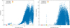 |
Fig. 2 Dynamical excitation of the planetesimal disk after the formation and migration of V1298 Tau b and e in scenario 9 from Table 3. Left panel: Eccentricity. Right panel: inclination. The empty circles in the panels mark the initial position of the giant planets. The simulation stopped with the giant planets about three times more distant from V1298 Tau than their current orbits to prevent dynamical instabilities that would result in a system incompatible with V1298 Tau’s compact architecture. |
4.2 Impact of the formation tracks of V1298 Taub and e on the subsequent evolution of the system
As shown in Fig. 2, the migration histories of V1298 Tau b and e shape the characteristics of the surviving planetesimal disk in two ways. First, the two migrating giant planets leave in their wake surviving planetesimal disks that are characterized by two different dynamical regions (see Fig. 2). The innermost region, roughly extending from the current orbits of the giant planets to the initial formation region of V1298 Tau b (see Fig. 2), is depopulated of planetesimals. Furthermore, due to the higher gas density in the inner disk regions, the dynamical excitation of the surviving planetesimals is efficiently damped by gas drag. The outermost region, roughly extending between the initial formation regions of V1298 Tau b and e (see Fig. 2), is populated by dynamically excited planetesimals.
Second, the larger migration of V1298 Tau e favors its acquisition of a marked population of Trojan satellites (see the planetesimals “piled up” on V1298 Tau e in Fig. 2), planetesimals co-orbiting with the giant planet in stable orbits around its L4 and L5 Lagrangian points with the star, which is similar to what is argued in the case of the Solar System for Jupiter (Pirani et al. 2019). The formation history of V1298 Tau b appears to hinder its efficiency in capturing Trojan satellites, although this could be an artefact of the specific migration tracks we adopted. Dedicated studies of the convergent migration and resonant trapping of V1298 Tau b and e are required to assess the dynamical lifetime of possible Trojan bodies.
The population of dynamically excited planetesimals created by the forming giant planets can affect the later evolution of the planetary system in two ways. On the one hand, the resulting higher impact frequency among planetesimals promotes the growth of existing oligarchs and the formation of additional massive planetary bodies, whose mutual interactions can inject them on eccentric orbits outside the present orbits of the four known planets. Later encounters between such excited outer planets and the four resonant inner planets could result in the breakup of the resonant chain and the onset of dynamical instability. On the other hand, the high-velocity impacts between the excited planetesimals cause large-scale production of collisional dust, replenishing the dust population of the circumstellar disk, as shown by the results of Turrini et al. (2019) and Bernabò et al. (2022).
We used the DEBRIS code (Turrini et al. 2019; Bernabò et al. 2022) to estimate the possible amount of collisional dust produced in simulations 4 and 9 (see Table 3 and Fig. 2 for the excited planetesimal disk at the end of simulation 9) by the migration of the V1298 Tau b and e. We assumed the plan-etesimal population to be characterized by the size-frequency distribution and mechanical strength typical of primordial plan-etesimals formed by streaming instability (Krivov et al. 2018; Turrini et al. 2019). We refer the interested reader to Turrini et al. (2019) and Bernabò et al. (2022) for details on the collisional and dust production algorithms implemented in the DEBRIS code.
The collisional cascade among the surviving excited plan-etesimals is capable of converting back into dust between 50 M⊕ (simulation 4) and 160 M⊕ (simulation 9). Such an amount of collisional dust, while drifting inward toward the star, is large enough to impact the formation history of V1298 Tau’s system. First, it promotes pebble accretion on surviving planetary embryos not accreted by the migrating planets, resulting in the formation of additional massive planets. We discuss the role of such planets in shaping the current architecture of V1298 Tau in Sect. 4.4. Second, it promotes new phases of streaming instability and can form massive planetesimal belts outside the current orbits of V1298 Tau e. The gravitational interactions between such belts and V1298 Tau’s four resonant planets can also potentially break the resonance chain. We investigate this scenario in Sect. 4.5.
4.3 Primordial capture in four-body resonance as V1298 Tau’s original architecture
As discussed in Sect. 2.1, the current architecture of V1298 Tau’s planets is not characterized by the resonant chain expected for such compact systems and shows the signs of having been sculpted by dynamical instabilities. To understand the origin of these characteristics, we first explored the possible primordial architectures of the system. There are two possible Laplace resonance chains that are dynamically close to the nominal solution and stable. They are the 3:2, 2:1, 3:2 chain and the 3:2, 2:1, 2:1 chain.
A possible scenario for the formation of either of the two resonant chains is that the planets migrated into resonance while the circumstellar disk was still present which is consistent with the migration scenarios simulated in Sect. 4.1 to explain the density values of V1298 Tau b and e. The capture in both these Laplace resonances was simulated with the parallel version of the N-body integration code RADAU15 (Everhart 1985) described in Sect. 3.2 using exponential damping terms in the semimajor axis and eccentricity with e-folding times of 0.5 Ma.
The masses adopted for the planets b and e are the nominal ones of Table 1, while for planets c and d, we considered two configurations (see Sect. 3.2): first, one configuration where the planets have a density of ρ = 0.65 g cm−3 and masses mc = 0.045 MJ and md = 0.077 MJ, and a second one where they have a density of ρ = 1.3 g cm−3 and masses mc = 0.09 MJ and md = 0.15 MJ. We found no significant differences between the two configurations.
The way in which the real capture in resonance may have occurred depends on a large number of parameters, including the initial orbits of the planets, the disk gas density profile and the timescale of its dissipation, the local effects of the planets on the gas, and the viscosity of the disk and its temperature profile. As it is impossible to perform a complete exploration of all these parameters, we first found a case in which the trapping occurs to confirm that it is indeed a realistic scenario.
Then, starting from this single case, we explored the phase space near this resonant solution in order to find all the possible resonant configurations. This approach allowed us to map the range of the planetary orbital elements in the specific Laplace resonant configuration. A random search without the knowledge of the orbital elements of at least one resonant configuration would be impossible. Depending on the above-mentioned parameters influencing the planet migration rate, different resonant configurations, among those we have found, were achieved during the evolution of the system.
The detailed exploration of the resonant phase space was performed by randomly sampling all planetary orbital elements in the proximity of the resonant solution. During the numerical integration of the planetary orbits, the critical angles of the Laplace resonance were automatically checked, and the non-librating, non-apsidal corotation cases were rejected. This last condition was dictated by the results of Beaugé et al. (2006), which suggest that as long as the migration is sufficiently slow to be approximated as an adiabatic process, all captured planets must be in apsidal corotations. The range we found in eccentricity shows the possible final orbital configurations of the four planets at the end of migration and resonance capture for different potential initial disk and planet parameters.
In Fig. 3, we illustrate the trapping in the 3:2, 2:1, 3:2 resonant chain where at the beginning of the simulation, the planets are close to the resonance and become captured during the subsequent inward migration. The eccentricity of each planet at the resonance trapping is pumped up to a value that is kept constant until the end of the migration. These high values are compatible with observations. The critical arguments of the three individual resonances librate around different values. In Fig. 4, we show the second scenario of resonance trapping where the planets are captured in a 3:2, 2:1, 2:1 resonant chain. Even in this case, the eccentricity is pumped up, and the resonant angles are all librating. We note that these simulations can be scaled in semimajor axis to get as close as possible to the observed semimajor axes of the planets.
In subsequent detailed explorations of the phase space, we numerically integrated millions of initial planetary configurations to find the extension of the phase space of the Laplace resonant configurations. In Fig. 5, we show the ranges of the initial values of semimajor axis (very tiny) and eccentricity with all four planets locked in a Laplace resonance in both cases (3:2, 2:1, and 3:2 on the left and 3:2, 2:1, and 2:1 on the right). Within these ranges, there are resonant solutions that are compatible in terms of eccentricity with the observed nominal system, suggesting that the primordial system was indeed in a Laplace resonance, and it later escaped from the resonant configuration. When comparing the two different configurations, 3:2, 2:1, and 3:2 versus 3:2, 2:1, and 2:1, we find it interesting to note that the last configuration leads to higher eccentricities for the third planet.
It is worth pointing out that the resonant solutions plotted in Fig. 5 were obtained by requiring that both resonant arguments librate, a condition naturally leading to apsidal libration. This condition is in agreement with the work of Beaugé et al. (2006), who suggest that as long as the orbital migration is sufficiently slow to be approximated by an adiabatic process (which is a condition compatible with the slow migration of giant planets toward the end of their formation; see e.g., Pirani et al. 2019; Tanaka et al. 2020), all captured planets should be in apsidal co-rotations.
Even if the resonant lock provides a solution for the origin of V1298 Tau’s compact architecture, the system is not in resonant chain at present, as confirmed by the extensive parameter exploration performed by Tejada Arevalo et al. (2022). The ratios between the planetary semimajor axes, according to the current nominal solutions from Table 1, are 1.312, 1.559, and 1.535, while to be in a four-body resonance, they should be 1.310, 1.587, and 1.310 or 1.310, 1.587, and 1.587.
This mismatch can be explained if the system evolved into either of the two resonant chains in the initial stages of its formation history but the resonance lock was broken during its later evolution by some additional dynamical mechanism. According to the capture simulations with a dissipating disk (Fig. 3 and Fig. 4), it is difficult for the gas dispersal alone to break the resonance lock. Dynamically destabilizing mechanisms must be invoked, specifically the planet-planet scattering and planetesimals scattering introduced in Sect. 4.1 and explored in detail in the next sections.
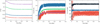 |
Fig. 3 Migration of the four planets in resonant configuration with the planets in the 3:2, 2:1, and 3:2 resonances. The left panel shows the semimajor axis evolution, the middle panel shows the eccentricity, and the right panel shows the resonant critical angles during the migration and subsequent resonance capture. The gas was slowly dissipating across the simulation. |
4.4 V1298 Tau’s present architecture: Resonance break by planet-planet scattering
The first possible scenario to break the resonant lock requires that additional dynamically excited planets populated, and maybe still populate, the system on orbits external to that of planet e. These excited planets would be difficult to detect through transits due to their longer orbital periods. As discussed in Sect. 4.2, the convergent migration shaping the formation path of V1298 Tau could act to promote the formation of such planets. These additional planets would have formed at later times in the wake of the passage of V1298 Tau b and e (see Sect. 4.2) and would not have migrated as close to the star as planets b and e either because of the dissipation of the gaseous disk or because they began to interact gravitationally with each other (Marzari et al. 2010). The dissipation of the disk itself can cause the onset of the dynamical instability among the resulting population of planets.
During their mutual gravitational interactions, one (or more) of such outer planets may have ended up in a highly eccentric orbit (Weidenschilling & Marzari 1996; Rasio & Ford 1996; Lin & Ida 1997 and Davies et al. 2014 for a review of the dynamical process and Limbach & Turner 2015; Zinzi & Turrini 2017; Turrini et al. 2020, 2022 for its signatures in observed multiplanet systems). This additional planet on an eccentric orbit may have become close enough to the four presently discovered planets while they were locked in a Laplace resonance to destabilize them. Encounters between this additional planet and planet e would break the resonance chain, leading the system of inner planets to instability on short timescales. The young age of the system suggests that the event triggering the instability of the outer planets, from which the fifth planet originated, could have been the dissipation of the gaseous disk, unless the planet formed directly on an eccentric orbit from the planetesimal disk after it was excited by the migration of planets b and e.
In Fig. 6, we show two examples of such a planet-planet scattering scenario. In the first case (top panel), a 200 M⊕ planet is added to the system on an orbit with a = 8 au, e = 0.95, and i = 10°. The inner planets remain locked in the four-body resonance until a series of close encounters with the fifth planet breaks the resonance lock, the critical arguments begin to circulate, and the system is quickly destabilized. In the second case (bottom panel), a heavier planet with M = 2MJ is placed on an orbit with a semimajor axis a = 4 au, eccentricity e = 0.85, and inclination i = 2°, and a similar evolution is observed.
These two examples are representative of the large sample of simulations we performed including outer planets with masses ranging from m = 150 M⊕ to m = 2 MJ and different initial eccentricities and semimajor axes, all leading to resonance break and instability. The first case has a very high eccentricity, which compensates the lower planet mass and the larger semimajor axis. It illustrates a scenario where the outer planetary system formed far away from the inner one and, becoming unstable, produced the perturbing planet. In the second case, the perturbing planet is closer but with a smaller eccentricity and a larger mass, representing a scenario where the inner and outer planets were potentially born more packed.
There is an infinite number of possible configurations of a perturbing planet on a crossing orbit with respect to the inner bodies leading to planet-planet scattering, chaotic evolution, and instability. Due to the chaotic nature of the problem, there is little reason to perform more extended explorations of the parameter space, particularly since our goal is solely to prove that this is a viable scenario. There is no way to identify the exact configuration that led to the present planetary system, as even those closely reproducing the observed system would not be unique. The timescale for the onset of instability depends on the initial conditions and can be tuned by changing the initial semimajor axis of the fifth planet to delay the instability.
This behavior can explain why at present we observe V1298 Tau’s four planets close to a resonance chain but not locked in it and is supported by the high value of the NAMD of V1298 Tau (see Sect. 2), which is highly suggestive of a period of violent planetary encounters (Carleo et al. 2021; Turrini et al. 2022). Unfortunately, it is not possible to trace back the initial conditions that led to the present unstable system with precision, even with a large sample of numerical simulations. The chaotic evolution due to planet-planet scattering can drive any putative system close to the observed one at different times during its evolution, and many different initial conditions can bring the system close to the observed one.
A possible alternative mechanism that may drive a system initially formed in a resonant chain to instability is tidal eccentricity damping, which may lead to divergence of the orbital semimajor axes of the resonant bodies (Batygin & Morbidelli 2013; Lithwick & Wu 2012). However, the eccentricity damping timescale of the innermost planet (planet c) is two orders of magnitude longer than the age of the system according to an estimate based on the tidal model of Leconte et al. (2010) and a modified tidal quality factor of 105 for the planet. The mass loss of the innermost planets due to photoevaporation, caused by their proximity to the star, is an additional plausible candidate for triggering dynamical instabilities in a packed resonant chain (Goldberg et al. 2022). Unfortunately, to be effective, this mechanism also requires a timescale that is on the order of 100 Ma or more, which is significantly greater than the age of V1298 Tau (see Sect. 2 and Table 1). Finally, it is worth noting that the two inner planets are also very close to a 2:1 resonance, and it is the third that is far from the resonant ratio with respect to the inner two.
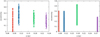 |
Fig. 5 Random resonant solutions in the semimajor axis and eccentricity planet for the two different chains (3:2, 2:1, and 3:2 on the left and 3:2, 2:1, and 2:1 on the right). The solutions are scalable in semimajor axes, and the three inner planet semimajor axes can be shifted until they coincide with the observed ones. |
4.5 V1298 Tau’s present architecture: Planetesimal scattering does not break the resonance
We also investigated the possibility that residual planetesimal scattering may be responsible for the resonant chain breaking and the current unstable configuration of the system. Remnant planetesimals may be present in the region where the planets migrate while in resonance. Furthermore, as discussed in Sect. 4.2, the migrating giant planets leave in their wake dynamically excited planetesimals whose high-velocity impacts convert a significant fraction of their mass into second-generation dust and pebbles (Turrini et al. 2012, 2019; Bernabò et al. 2022). While drifting toward the star, this second-generation dust can trigger new phases of planetesimal formation and create new planetesimal belts closer to the resonant planets.
We considered two scenarios characterized by planetesimal belts of 10 and 50 M⊕, respectively, both extending between 0.3 au and 10 au. This is the same orbital region where gas drag efficiently damps the dynamical excitation of the planetesimals (see Fig. 2), and as a result, the planetesimals populating the belts start their evolution after the dispersal of the circumstellar disk on low-eccentricity, low-inclination orbits (e ≈ i < 0.01, where the inclination is expressed in radians).
We simulated the 10 and 50 M⊕ planetesimal belts using 1000 massive particles whose initial masses are 0.01 and 0.05 M⊕, respectively. Collisions among planetesimals were treated as inelastic mergers resulting in mass growth. The giant planets were placed in a stable resonant chain at the beginning of the simulations, and the whole system was evolved for 10 Ma (i.e., the lower bound of V1298 Tau’s age in Table 1) with a timestep of 0.35 days. The simulations were performed using the GPU-accelerated version of Mercury-Arχes N-body code (Turrini et al. 2019, 2021) discussed in Sect. 3.2.
The simulations revealed that the presence of the 10 M⊕ planetesimal belt has negligible effects on the dynamical evolution of the four planets, whose orbital architecture remain unaltered with respect to the reference scenario with no planetesimal belt. The presence of the 50 M⊕ planetesimal belt produces limited alterations to the dynamical evolution of the planets, as the encounters with the more massive planetesimals slightly damp the eccentricity of V1298 Tau e and reduce the amplitude of the eccentricity oscillations of V1298 Taub. Aside from these limited differences, the secular variations of the orbital elements of the four planets are within the ranges of the scenarios with the 10 M⊕ belt and no planetesimal belt. Overall, even the presence of the 50 M⊕ planetesimal belt does not appear capable of breaking the resonance chain over the lifetime of the system. Unless V1298 Tau hosts a planetesimal belt more massive than those considered in this analysis, planetesimal scattering does not appear as a viable solution to break the resonance chain.
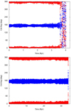 |
Fig. 6 Evolution of the critical argument of the outer planet pair (b and e) initially locked in a 3:2 resonance. In the upper panel, the additional planet has a mass m = 200 M⊕, a = 8 au, e = 0.95, and i = 10°. In the bottom panel, a more massive planet on a less eccentric orbit was adopted (m = 2 MJ, a = 4 au, e = 0.85, and inclination i = 2°). In both cases, after a period of chaotic evolution, the onset of repeated close encounters breaks the resonance lock and leads to fast instability. |
5 Observational clues on the presence of additional planets at wide separation
The scenario of high enrichment in heavy elements of V1298 Tau b and e we explore in Sect 4.1 is best reproduced if the two planets form and migrate across compact protoplanetary disks with a radial extension of <50–100 au. Wider disks imply lower spatial densities of the planetesimals, as the disk mass is spread over wider areas since, for the same total disk mass, they would have a lower coefficient of the power law describing the mass density profile. This, in turn, implies that migrating giant planets encounter fewer planetesimals and accrete lower masses of heavy elements over the same radial displacement.
Fitting the density values of planets b and e in such wide disks would require initial formation regions for the two planets similar to those of the giant planets revealed by ALMA surveys (e.g., Long et al. 2018; Andrews et al. 2018). However, it is currently unclear if such outer formation regions are capable of producing hot planets such as those around V1298 Tau. The presence of massive planets at large orbital separations, the signpost of an extended native disk, would therefore require revisiting the scenario discussed in Sect. 4.1.
Considering the young age of the system, the direct imaging technique allowed us to achieve sensitivities well into the planetary regime over a broad range of separations. Only moderately shallow data are available in the literature (Daemgen et al. 2015), so we observed V1298 Tau with SPHERE as part of a program on the characterization of the outer regions around young stars with transiting planets (Desidera et al., in prep.). The comparison of proper motions from different catalogs is also considered as an indicator of the possible presence of companions at moderately wide separations.
5.1 Observations and data reduction
We observed V1298 Tau three times with the SPHERE high-contrast imaging instrument at VLT (Beuzit et al. 2019). A first-epoch observation was acquired on 18 November 2019, exploiting the IRDIFS mode, then observing simultaneously with IFS (Claudi et al. 2008) in the Y and J bands (from 0.95 to 1.35 µm) and with IRDIS (Dohlen et al. 2008) in the H band using the H23 filter pair (wavelength of 1.593 µm and 1.667 µm for H2 and H3, respectively; Vigan et al. 2010). The second and third observations were obtained on 28 October 2021 and 2 December 2021, with the main goal of determining the status (physical companion versus background) of a faint candidate detected in the first epoch, as discussed in Sect. 5.2.
The follow-up observations were performed in the IRDIFS_EXT mode, then observing simultaneously with IFS in Y, J, and H bands (from 0.95 to 1.65 µm) and with IRDIS in the K band using the K12 filter pair (wavelength of 2.110 µm and 2.251 µm for K1 and K2 bands, respectively). We chose a different setup for the follow-up in order to obtain complementary photometric measurements for the candidate and achieve a better sensitivity for planets with very dusty atmospheres (see, e.g., Chauvin et al. 2018). The characteristics of the three datasets are summarized in Table 4.
The data were reduced through the SPHERE Data Center (Delorme et al. 2017) following the SPHERE Data Reduction and Handling pipeline (Pavlov et al. 2008) and applying the appropriate calibrations for our datasets. We then applied speckle subtraction algorithms TLOCI (Marois et al. 2014) and principal components analysis (PCA; Soummer et al. 2012) on the reduced data as implemented in the SpeCal pipeline (Galicher et al. 2018).
Main characteristics of the SPHERE observations of V1298 Tau used for this work.
Astrometry and photometry of the candidate companion detected around V 1298 Tau.
5.2 A background object projected close to V1298 Tau
A point source was detected in all the three epochs in the IRDIS field of view at a separation of about 2.77″ (Fig. 7). The source has a contrast higher than 11 magnitudes with respect to the central star. The signal-to-noise ratio of the detection is 35.2, 6.8, and 9.4 for the first, second, and third epochs, respectively. This difference is reflected by the higher error bars in the astrometry and the photometry of the candidate listed in Table 5. The astrometric calibration of each epoch was obtained following the method devised by Maire et al. (2016). The photometry was calculated using the negative planet method as described in Bonnefoy et al. (2011) and in Zurlo et al. (2014), for example.
We checked the NIRI images of Vl298Tau obtained by Daemgen et al. (2015), and we confirmed that the source is not detected in this dataset, as expected from the published detection limits. We compared the astrometry in the first and the third epoch, adopting the stellar parameters listed in Table 1. We decided to exclude the second epoch from this analysis as, in that epoch, the candidate companion is just above the detection limit and the astrometric error bars are very large as a consequence.
This comparison is displayed in Fig. 8, where the green square represents the position of the candidate relative to the star in the first epoch, while the orange diamond gives the relative position of the candidate in the third epoch. The solid black line represents the course of the candidate during the considered period if it were a background object with no proper motion. The black square at the end of this line is the expected position of the candidate in this latter case at the third epoch. This plot excludes the fact that the candidate could be gravitationally bound to the central star and points to it being a background object possibly possessing a non-negligible proper motion.
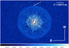 |
Fig. 7 SPHERE image of Vl298Tau in the H2 band with the faint background object at 2.77″ highlighted with the red arrow. |
5.3 Constraints on additional planets
No additional sources were detected either with IFS or IRDIS. In order to quantify our detection limits, we defined the contrast around the central star for both instruments and for the first and third epochs, exploiting the procedure described in Mesa et al. (2015) and corrected for the small sample statistic following the method described by Mawet et al. (2014). From these contrast limits, we calculated the upper mass limits for companions around V 1298 Tau using the AMES-COND models (Allard et al. 2003) and adopting the stellar parameters by Suárez Mascareño et al. (2022). Finally, we defined the best upper limits for all three epochs and considering both IFS and IRDIS mass limits. The final results of this procedure are displayed in Fig. 9.
The present constraints rule out the presence of giant planets more massive than Jupiter beyond 50-100 au (i.e., at orbital periods greater than 300–1000 years), suggesting that the circumstellar disk from which V1298 Tau’s planetary system formed was more compact and dense than those presently being observed by ALMA surveys (e.g., Andrews et al. 2018; Long et al. 2018). Such a compact disk fits the picture discussed in Sect. 4.1, as it favors the accretion of large amounts of planetesimals by the migrating planets and the production of large amounts of collisional dust from the surviving planetesimal disk.
Furthermore, the present constraints rule out only giant planets more massive than a few Jovian masses in the inner regions within 50 au. This means that between 10 and 50 au (i.e., at orbital periods between 30 and 300 yr), there may well be planets as massive as 2My on eccentric or unstable orbits that are below the detection limit of SPHERE (as discussed in Sect. 5.4, such planets would fall near or below the 50% iso-probability curve of Gaia’s astrometric observations). Among these planets, the one that possibly destabilized the inner four may be still orbiting V1298 Tau on a highly eccentric orbit, unless it was ejected from the system by the planet-planet scattering process that triggered the instability.
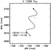 |
Fig. 8 Relative astrometric position of the proposed companion in the first and the last observing epoch. The solid black line represents the expected course of the companion if it were a stationary background object. The black square at the end of the line represents the expected position at the epoch of the last observation in this case. The minor difference between the observed and expected positions is consistent at ~1.5cr with measurement errors or could be due to a non-zero intrinsic motion of the background source. |
5.4 Additional clues from astrometry
The star V1298 Tau was not observed by the HIPPARCOS space astrometry mission, so it is not possible to provide direct constraints on long-period orbiting companions in a regime of orbital separations complementary to the one probed by the SPHERE direct imaging observations (a ≲ 10 au) using the HIPPARCOS-Gaia proper motion anomaly technique (see, e.g., Kervella et al. 2019, 2022; Brandt 2018, 2021). However, Gaia DR3 provides the renormalized unit weight error (RUWE) statistics, which is a good proxy for the quality of the single-star astrometric solution. Typically, RUWE ≃ 1.0 indicates a good-quality single-star solution, while sources with RUWE above the threshold value ≃1.4 are typically considered to have observations inconsistent with the astrometric five-parameter model, with additional variability in the astrometry possibly due to binarity (e.g., Lindegren et al. 2018, 2021).
The reported RUWE value for V1298 Tau in Gaia DR3 is 1.035, which indicates no significant departures from a singlestar model are observed, and in fact no non-single-star solution of any type has been reported. Following the approach by Belokurov et al. (2020) and Penoyre et al. (2020), for example, it is nevertheless possible to explore the regime of companion masses and orbital separations that can be excluded, as they would have produced larger RUWE values than the reported one.
We set up a numerical simulation, creating synthetic Gaia observations of V1298 Tau using the nominal astrometric parameters published in Gaia DR3. We used the Gaia observation forecast tool4 to obtain a close representation of the actual Gaia observation times, scan angle, and along-scan parallax factors encompassing the mission time span utilized in Gaia DR3. Orbital motion effects were linearly superposed considering companions with orbital periods in the range 0.5–20.0 yr and masses in the range 1.0–40.0 MJ.
For each period-mass pair, 100 random realizations of the remaining orbital elements were produced, all being drawn from uniform distributions within their nominal intervals. The Gaia-like observations of each star plus companion system were then perturbed with Gaussian measurement uncertainties appropriate for the case of a G = 10 mag star such as V1298 Tau (see, e.g., Holl et al. 2023, Fig. 3). Each time series was then fitted with a single-star model, and the corresponding RUWE value was recorded. For each period-mass pair, the fraction of systems with RUWE values exceeding the one reported for V1298 Tau in the Gaia DR3 archive was recorded. In total, the simulation was run for 4 000 000 systems.
Figure 10 shows the iso-probability contours in companion period-mass space corresponding to different fractions of systems for which RUWE was recorded to be larger than the value reported in the Gaia DR3 archive for V1298 Tau. Given the time span and quality of Gaia DR3 observations for the star, we deduced that the Gaia sensitivity to super-Jupiter-type companions around V1298 Tau is presently limited to a narrow regime of orbital periods in the approximate interval of 1.5–4 yr, or roughly 1.4–2.7 au. This is the regime of orbital separations for which Gaia DR3-level astrometry provides mass sensitivity comparable to that achieved by SPHERE’S direct imaging data at 10–20 au.
The astrometric signals of the much shorter-period giants V1298 Tau b and e are clearly out of reach for Gaia, as expected. In the approximate period interval 5–10 yr, the presence of low-mass brown dwarfs can be safely ruled out. At P = 20 yr, a 20-MJ companion still has a 50% chance of going undetected. As in the case of SPHERE’S observations, Gaia’s astrometric data leave open the possibility that planets as massive as 2MJ linked to the destabilization of the primordial resonant chain of V1298 Tau’s four inner planets still orbit the host star on eccentric or unstable orbits below the detection limits.
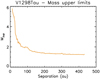 |
Fig. 9 Mass detection limits (5σ) obtained from the SPHERE data (both IRDIS and IFS) expressed in units of Jovian mass as a function of the separation expressed in astronomical units. |
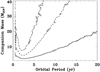 |
Fig. 10 Gaia DR3 sensitivity to companions of a given mass (in units of Jovian mass) as a function of the orbital period (in years). Solid, dashed, and dashed-dotted lines correspond to iso-probability curves for 50%, 90%, and 99% probability of a companion of given properties to produce a RUWE value that exceeds the value reported in the Gaia DR3 archive (1.035). |
5.5 Additional clues from radial velocities
To further constrain the presence of additional companions, we investigated the detection limits from the RV time series from Suárez Mascareño et al. (2022) through the Bayesian procedure adopted in Pinamonti et al. (2022). This technique consists of modeling an additional planetary signal in the RV time series by means of the publicly available emcee Affine Invariant MCMC Ensemble sampler (Foreman-Mackey et al. 2013) and using the posterior distribution of its orbital parameters to derive the detectability function.
The additional planet was modeled simultaneously to the other planetary signals present in the data, both to account for their uncertainties and to accurately estimate its detectability. However, the strong stellar activity contamination in the RV hinders a straightforward computation of the detection function of the time series. This issue can be addressed by adopting the RV residuals from Suárez Mascareño et al. (2022), as the activity have already been removed, or by including it in the analysis via GP regression (see Pinamonti et al. 2022). The first approach produces an optimistic detection threshold, while the second yields a pessimistic one, as illustrated in the left panel of Fig. 11.
The detection function can be reliably computed with the Bayesian technique only for periods up to the time span of the RV observations (≃400 days). To extend the search to longer periods, comparable with those investigated in Sects. 5.3 and 5.4, we performed an injection-recovery simulation in which synthetic planetary signals were injected in the RV residuals and the detection function was computed as the recovery rate of these signals, covering orbital periods between 400–4000 days (i.e., approximately between 1 and 5 au). The simulated signals were fit with either a circular-Keplerian orbit or a linear or quadratic trend (because a period longer than the time span might not be properly modeled by a Keplerian). We adopted the Bayesian information criterion (BIC; Schwarz 1978) in order to compare the fitted planetary model with a constant model with a threshold of ΔBIC > 10. The resulting detection function map is shown in the right panel of Fig. 11.
As can be seen from Fig. 11, in the optimistic case and considering the best-case correction of the stellar activity, we can rule out the presence of companions of 0.5MJ at periods shorter than P = 650 d, and we can rule out the presence of additional companions as massive as 2MJ up to P = 1500 d. However, when considering the pessimistic case and taking into account the effect of the stellar noise in the RV time series, we can exclude only the presence of 2MJ companions on short-period orbits (P ≲ 3 d). The real detection limit of V1298 Tau likely falls between these two scenarios. As a result, while we can somewhat confidently rule out the presence of massive companions at orbits close to those of the transiting planets, it is difficult to accurately constrain the presence of longer-period planetary signals underneath the stellar RV noise.
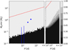 |
Fig. 11 Detection function map of the RV time series of V1298 Tau from Suárez Mascareño et al. (2022), with the stellar activity already removed (i.e., the optimistic case). The color scale expresses the detection function, while the red dashed lines correspond to the 90% detection threshold including the stellar activity in the modeling (i.e., the pessimistic case). The blue circles correspond to the position of the measured planets in the systems, while the blue lines mark the upper limits of the planets with no mass-measurement yet. The left panel shows the Bayesian detection map computed for P < 400 days, while the right panel shows the inject-recovery detection map computed for 400 < P < 4000 days. |
6 Discussion and conclusions
The recent observational campaigns aimed at characterizing the planets around V1298 Tau (David et al. 2019a,b; Suárez Mascareño et al. 2022; Feinstein et al. 2022; Damasso et al. 2023) reveal that this young planetary system is highly peculiar. Its current architecture is quite compact, yet its planets do not appear to be globally locked in resonance Tejada Arevalo et al. (2022), and their orbital characteristics argue for the system having crossed phases of dynamical instability (Sect. 2.1).
The dynamical state of the system, however, is not the sole peculiar aspect of V1298 Tau. The estimated masses of its two outer giant planets are associated with anomalously high density values for such young planetary objects. The confirmation of its currently assessed physical characteristics would make V1298 Tau a unique natural laboratory to study the formation and evolution of planetary systems as well as a compelling target for future physical and atmospheric characterization campaigns.
Specifically, unless young giant planets contract faster than previously thought (Suárez Mascareño et al. 2022), the current densities of V1298 Tau b and e point to their formation tracks as being shaped by large-scale migration and enrichment in heavy elements (Thorngren et al. 2016; Shibata et al. 2020; Turrini et al. 2021; Pacetti et al. 2022). Consequently, reconstructing the formation history of V1298 Tau must account for both the high enrichment of heavy elements in its outer two planets and the non-resonant state of the compact dynamical configuration of the system.
In this work, we outlined the possible sequence of events that drove the system into its present configuration. Specifically, we argued that the convergent, large-scale migration of V1298 Tau’s planets while embedded in their native circumstellar disk can explain both the density values of the two outermost giant planets and the formation of V1298 Tau’s compact architecture by resonant trapping. The dynamically excited planetesimal disk left behind by the migrating giant planets can then support the formation of additional planets that can break the original resonant chain.
6.1 Assembling the mosaic of V1298 Tau’s formation history
The uncertainty affecting the mass and density estimates of V1298 Tau’s planets make it difficult to precisely pinpoint their formation regions. Optimistic estimates require about 20 and 30 M⊕ of heavy elements for V1298 Taub and e, respectively. Accounting for the lower density of the hot gas composing such young giant planets brings the masses of heavy elements to 90 and 110 M⊕, respectively, making these planets some of the most metallic gas giants currently known. Adopting the nominal mass of V1298 Tau e would result in a planet whose composition is two-thirds heavy elements, and therefore more similar to Neptune than jupiter, notwithstanding its jovian mass.
Explaining the nominal density of V1298 Tau e in the framework of the migration and enrichment scenario would require the planet to have undergone extreme migration within a massive circumstellar disk. The intense planetesimal flux hitting the forming planet would likely hinder the onset of its runaway gas accretion process. This would keep the planet in the form of a massive core surrounded by an extended atmosphere (unless the primordial atmosphere is collisionally stripped) until the planetesimal flux drops and the gas accretion process can restart.
A similar scenario is discussed for jupiter by Alibert et al. (2018), but the characteristics of V1298 Tau e would invoke a significantly more extreme version than its original formulation. This scenario would make V1298 Tau e the first example of a new class of outcomes of the planet formation process. Due to the large uncertainty on its mass, however, it is more plausible that the true density of V1298 Taue is lower than its current nominal value. Alternatively, the high density can be explained by invoking the interplay between planetesimal accretion and the accretion of disk gas enriched in heavy elements (Booth & Ilee 2019; Cridland et al. 2019; Schneider & Bitsch 2021).
Notwithstanding these uncertainties, our results describe an overall coherent picture. Our simulations of the accretion history of V1298 Tau b and e show that to reproduce their enrichment in heavy elements, particularly that of planet e, their native circumstellar disk was plausibly massive, at least as massive as 0.1 times the host star. While massive, such a disk should have been compact, with radial extension not exceeding 50–100 au. This is consistent with the lack of massive companions at large separations that we verified by combining SPHERE’s direct imaging and Gaia’s astrometric data.
Both planets must have crossed significant fractions of this disk to accrete enough heavy elements to fit the current data, as when adopting even the lowest metallicity values, their formation region lies beyond jupiter’s current orbit. In all of our simulations, V1298 Taue should have started its formation about twice as far as V1298 Tau b to be able to encounter and accrete enough planetesimals. Depending on their real density values and the interplay between planetesimal and enriched-gas accretion in delivering heavy elements, their migration could have spanned from a few astronomical units to several tens of astronomical units. This uncertainty showcases the limited diagnostic power of planetary density and metallicity (see Turrini et al. 2022 for more discussion) but also makes these planets compelling targets for future atmospheric characterization, as we discuss below (see Sect. 6.2).
Fitting V1298 Tau’s current compact architecture with the large-scale migration of its two outer planets requires that the system formed by convergent migration and resonant trapping (i.e., the planets were trapped in a sequence of mean motion resonances while migrating inwards due to disk-planet interactions). This is confirmed by our simulations showing how the planets are captured in a Laplace resonance in the presence of dissipative forces such as those caused by their interactions with the native circumstellar disk. The resonance trapping mechanism naturally explains why at present V1298 Tau’s four planets are very close to a resonant configuration. Moreover, their convergent migration promotes the conditions for the late formation of massive planets in their wake, an important piece to explain the later evolution of the system.
Resonant capture can account for the high eccentricity of the planets, which will be excited during the dissipative resonant capture. However, since the present system is only close to but not in a Laplace resonance (Tejada Arevalo et al. 2022) and also in a dynamically excited state, some additional mechanism is needed to break the resonance lock after its formation. Thanks to its well-constrained young age, V1298 Tau is an almost unique laboratory for exploring different resonance-breaking mechanisms. Specifically, V1298 Tau’s age allows for the exclusion of both the mechanism proposed by Batygin & Morbidelli (2013) and a possible role of planetary evaporation (see Goldberg et al. 2022).
Next, we explore the two remaining possibilities we identified: planetesimals scattering and planet-planet scattering. In the case of planetesimals scattering, we verified with N-body simulations that even massive planetesimal populations made by the combination of remnant and second-generation bodies cannot break the tight resonant lock. In the case of planet-planet scattering, we find that a planet with a mass ranging from 0.5 to 2 MJ on highly eccentric orbits and with a semimajor axis between 4 and 8 au can break the resonance lock after a series of close encounters with the inner planets and leave the inner planetary system in a dynamical state like the one observed at present.
The planet-planet scattering mechanism requires that the multiplicity of V1298 Tau’s planetary system is or was higher than that suggested by its currently discovered four planets. The massive planets required by this mechanism are below the detection thresholds of the current SPHERE and Gaia observations, meaning that the eccentric planets responsible for breaking the resonant lock could still be orbiting V1298 Tau. As we showed, the possibility that one or more additional planets formed in V1298 Tau’s circumstellar disk is supported by the formation scenario we proposed to explain the architecture and density values of V1298 Tau’s four inner planets.
In other words, the very same conditions required to produce the densities of planets b and e as well as the compact architecture of V1298 Tau by means of a resonance lock plant the seed for destroying the said lock. Additional observations are needed to conclusively characterize the dynamical state of V1298 Tau’s four planets, identify the possible presence of the outer planet(s), and verify whether they could have been responsible for breaking the original resonance lock of the inner four planets.
6.2 Implications for the atmospheric compositions of V1298 Taub and e
As introduced above, the unusual formation history of V1298 Tau makes this young system a compelling target for future observational studies of atmospheric composition, notwithstanding the challenges posed by the activity of its host star. While the uncertainty of the mass and density values of V1298 Tau b and e hinder any attempt to pinpoint their original formation region through metallicity alone, the different densities of the two planets provide a basis to argue that their atmospheric compositions should be markedly different.
As an example, for the disk thermal profile we adopted in our simulations, the snowlines of H2O, CO2, and CO would be located at about 2, 6, and 23 au, respectively, while those of NH3 and N2 would fall at about 4 and 30 au (e.g., Eistrup et al. 2016; Öberg & Wordsworth 2019). Most refractory elements would be in solid form already within 1 au (e.g., Lodders 2003; Fegley & Schaefer 2010). The atmospheric composition of V1298 Tau b and e would therefore be characterized by radically different elemental abundances, depending on their actual formation tracks (e.g., Turrini et al. 2021; Pacetti et al. 2022; Fonte et al. 2023).
Specifically, the lowest metallicity scenario we considered would place the formation of both planets inside the CO snowline. The presence of massive cores inside both planets or, alternatively, lower masses and densities than their current modal values would reduce the planetesimal mass to be accreted and would shift their formation regions closer or inside the H2O, NH3, and CO2 snowlines. Adopting more realistic gas densities for such hot and young objects would place the formation region of both planets beyond the CO snowline, with V1298 Tau e plausibly having formed beyond the N2 snowline. The nominal metallicity scenario for V1298Taue, which is also its highest metallicity scenario, firmly puts the formation region of the planet beyond the N2 snowline. These different formation regions would be reflected by different patterns in the abundance ratios between C, O, and N (see Turrini et al. 2021, 2022; Pacetti et al. 2022 and Biazzo et al. 2022; Kolecki & Wang 2022 for observational validations).
Finally, the highest metallicity scenario for V1298Taue requires an extreme planetesimal accretion history, unless the giant planet accreted gas enriched in heavy elements from the disk (Booth & Ilee 2019; Cridland et al. 2019; Schneider & Bitsch 2021). Such a process results in a lower refractory-to-volatile ratio and a different C/O ratio than those resulting from the sole accretion of planetesimals (Turrini et al. 2021; Schneider & Bitsch 2021; Pacetti et al. 2022). Constraining the abundance of one or more refractory elements in V1298 Tau e’s atmosphere would allow these two sources of heavy elements to be distinguished (Turrini et al. 2021; Pacetti et al. 2022) as well as possible biases affecting the C/O ratio due to the depletion of atmospheric oxygen by refractory species to be identified (Fonte et al. 2023).
Acknowledgements
This work has made use of the SPHERE Data Centre, jointly operated by OSUG/IPAG (Grenoble), PYTHEAS/LAM/CeSAM (Marseille), OCA/Lagrange (Nice), Observatoire de Paris/LESIA (Paris), and Observatoire de Lyon/CRAL, and supported by a grant from Labex OSUG2020 (Investissements d’avenir – ANR10 LABX56). This work has also made use of data from the European Space Agency (ESA) mission Gaia (https://www.cosmos.esa.int/gaia), processed by the Gaia Data Processing and Analysis Consortium (DPAC, https://www.cosmos.esa.int/web/gaia/dpac/consortium). Funding for the DPAC has been provided by national institutions, in particular the institutions participating in the Gaia Multilateral Agreement. The authors acknowledge the support of the National Institute of Astrophysics (INAF) through the PRIN-INAF 2019 projects “Planetary systems at young ages (PLATEA)” and “The HOT-ATMOS Project”, as well as that of the Italian Space Agency (ASI) through the ASI-INAF contracts no. 2018-16-HH.0 and 2021-5-HH.0, and that of the European Research Council via the Horizon 2020 Framework Programme ERC Synergy “ECOGAL” Project GA-855130. This work is supported by the Fondazione ICSC, Spoke 3 “Astrophysics and Cosmos Observations”, National Recovery and Resilience Plan (Piano Nazionale di Ripresa e Resilienza, PNRR) Project ID CN_00000013 “Italian Research Center on High-Performance Computing, Big Data and Quantum Computing” funded by MUR Missione 4 Componente 2 Investimento 1.4: Potenziamento strutture di ricerca e creazione di “campioni nazionali di R&S (M4C2-19)” -Next Generation EU (NGEU). D.T. acknowledges the support of the INAF Main Stream project “Ariel and the astrochemical link between circumstellar discs and planets” (CUP: C54I19000700005). D.P. acknowledges the support from the Istituto Nazionale di Oceanografia e Geofisica Sperimentale (OGS) and CINECA through the program “HPC-TRES (High Performance Computing Training and Research for Earth Sciences)” award number 2022-05. A.S. acknowledges support from the Italian Space Agency (ASI) under contract 2018-24-HH.0 “The Italian participation to the Gaia Data Processing and Analysis Consortium (DPAC)” in collaboration with the Italian National Institute of Astrophysics. A.S.M. acknowledges financial support from the Spanish Ministry of Science and Innovation (MICINN) under 2018 Juan de la Cierva program IJC2018-035229-I. A.S.M. and J.I.G.H. acknowledge financial support from the Spanish Ministry of Science and Innovation (MICINN) project PID2020-117493GB-I00, and from the Government of the Canary Islands project ProID2020010129. V.B. and N.L. acknowledge support from the Agencia Estatal de Investigación del Ministerio de Ciencia e Innovación (AEI-MCINN) under grant PID2019-109522GB-C53. C.d.B. acknowledges support by Mexican CONAHCYT research grant FOP16-2021-01-320608. The computational resources for this work were supplied by the Genesis cluster at INAF-IAPS and the technical support of Romolo Politi, Scigè john Liu and Sergio Fonte is gratefully acknowledged.
References
- Alibert, Y., Venturini, J., Helled, R., et al. 2018, Nat. Astron., 2, 873 [NASA ADS] [CrossRef] [Google Scholar]
- Allard, F., Guillot, T., Ludwig, H., et al. 2003. IAU Symp., 211, 325 [NASA ADS] [Google Scholar]
- Andrews, S. M., & Williams, J. P. 2007, ApJ, 659, 705 [NASA ADS] [CrossRef] [Google Scholar]
- Andrews, S. M., Huang, J., Pérez, L. M., et al. 2018, ApJ, 869, L41 [NASA ADS] [CrossRef] [Google Scholar]
- Asplund, M., Grevesse, N., Sauval, A. J., & Scott, P. 2009, ARA & A, 47, 481 [NASA ADS] [CrossRef] [Google Scholar]
- Atreya, S. K., Crida, A., Guillot, T., et al. 2018, in Saturn in the 21st Century, eds. K. H. Baines, F. M. Flasar, N. Krupp, & T. Stallard (Cambridge University Press), 5 [CrossRef] [Google Scholar]
- Batygin, K., & Morbidelli, A. 2013, AJ, 145, 1 [NASA ADS] [CrossRef] [Google Scholar]
- Beaugé, C., Michtchenko, T. A., & Ferraz-Mello, S. 2006, MNRAS, 365, 1160 [Google Scholar]
- Belokurov, V., Penoyre, Z., Oh, S., et al. 2020, MNRAS, 496, 1922 [Google Scholar]
- Benatti, S., Nardiello, D., Malavolta, L., et al. 2019, A & A, 630, A81 [CrossRef] [EDP Sciences] [Google Scholar]
- Benatti, S., Damasso, M., Borsa, F., et al. 2021, A & A, 650, A66 [NASA ADS] [CrossRef] [EDP Sciences] [Google Scholar]
- Bernabò, L. M., Turrini, D., Testi, L., Marzari, F., & Polychroni, D. 2022, ApJ, 927, L22 [CrossRef] [Google Scholar]
- Beuzit, J. L., Vigan, A., Mouillet, D., et al. 2019, A & A, 631, A155 [NASA ADS] [CrossRef] [EDP Sciences] [Google Scholar]
- Biazzo, K., D’Orazi, V., Desidera, S., et al. 2022, A & A, 664, A161 [NASA ADS] [CrossRef] [EDP Sciences] [Google Scholar]
- Bitsch, B., Lambrechts, M., & Johansen, A. 2015, A & A, 582, A112 [CrossRef] [EDP Sciences] [Google Scholar]
- Bonnefoy, M., Lagrange, A. M., Boccaletti, A., et al. 2011, A & A, 528, L15 [NASA ADS] [CrossRef] [EDP Sciences] [Google Scholar]
- Booth, R. A., & Ilee, J. D. 2019, MNRAS, 487, 3998 [CrossRef] [Google Scholar]
- Borucki, W. J., Koch, D. G., Lissauer, J. J., et al. 2003, SPIE Conf. Ser., 4854, 129 [Google Scholar]
- Brandt, T. D. 2018, ApJS, 239, 31 [Google Scholar]
- Brandt, T. D. 2021, ApJS, 254, 42 [NASA ADS] [CrossRef] [Google Scholar]
- Brasser, R., Duncan, M. J., & Levison, H. F. 2007, Icarus, 191, 413 [NASA ADS] [CrossRef] [Google Scholar]
- Carleo, I., Benatti, S., Lanza, A. F., et al. 2018, A & A, 613, A50 [NASA ADS] [CrossRef] [EDP Sciences] [Google Scholar]
- Carleo, I., Malavolta, L., Lanza, A. F., et al. 2020, A & A, 638, A5 [NASA ADS] [CrossRef] [EDP Sciences] [Google Scholar]
- Carleo, I., Desidera, S., Nardiello, D., et al. 2021, A & A, 645, A71 [NASA ADS] [CrossRef] [EDP Sciences] [Google Scholar]
- Chambers, J. E. 2001, Icarus, 152, 205 [Google Scholar]
- Chauvin, G., Gratton, R., Bonnefoy, M., et al. 2018, A & A, 617, A76 [CrossRef] [EDP Sciences] [Google Scholar]
- Claudi, R. U., Turatto, M., Gratton, R. G., et al. 2008, Proc. SPIE, 7014, 70143E [Google Scholar]
- Coradini, A., Turrini, D., Federico, C., & Magni, G. 2011, Space Sci. Rev., 163, 25 [NASA ADS] [CrossRef] [Google Scholar]
- Covino, E., Esposito, M., Barbieri, M., et al. 2013, A & A, 554, A28 [NASA ADS] [CrossRef] [EDP Sciences] [Google Scholar]
- Cridland, A. J., van Dishoeck, E. F., Alessi, M., & Pudritz, R. E. 2019, A & A, 632, A63 [NASA ADS] [CrossRef] [EDP Sciences] [Google Scholar]
- Daemgen, S., Bonavita, M., Jayawardhana, R., Lafrenière, D., & Janson, M. 2015, ApJ, 799, 155 [NASA ADS] [CrossRef] [Google Scholar]
- Damasso, M., Lanza, A. F., Benatti, S., et al. 2020, A & A, 642, A133 [NASA ADS] [CrossRef] [EDP Sciences] [Google Scholar]
- Damasso, M., Scandariato, G., Nascimbeni, V., et al. 2023, A & A, in press, https://doi.org/10.1051/0004-6361/202346840 [Google Scholar]
- D’Angelo, G., Weidenschilling, S. J., Lissauer, J. J., & Bodenheimer, P. 2021, Icarus, 355, 114087 [CrossRef] [Google Scholar]
- David, T. J., Hillenbrand, L. A., Cody, A. M., Carpenter, J. M., & Howard, A. W. 2016, ApJ, 816, 21 [Google Scholar]
- David, T. J., Cody, A. M., Hedges, C. L., et al. 2019a, AJ, 158, 79 [NASA ADS] [CrossRef] [Google Scholar]
- David, T. J., Petigura, E. A., Luger, R., et al. 2019b, ApJ, 885, L12 [Google Scholar]
- Davies, M. B., Adams, F. C., Armitage, P., et al. 2014, in Protostars and Planets VI, eds. H. Beuther, R. S. Klessen, C. P. Dullemond, & T. Henning (Tucson: University of Arizona Press), 787 [Google Scholar]
- Delorme, P., Meunier, N., Albert, D., et al. 2017, in SF2A-2017: Proceedings of the Annual meeting of the French Society of Astronomy and Astrophysics, eds. C. Reylé, P. Di Matteo, F. Herpin, et al. [Google Scholar]
- Dohlen, K., Langlois, M., Saisse, M., et al. 2008, Proc. SPIE, 7014, 70143L [Google Scholar]
- Donati, J. F., Moutou, C., Malo, L., et al. 2016, Nature, 534, 662 [Google Scholar]
- Donati, J. F., Yu, L., Moutou, C., et al. 2017, MNRAS, 465, 3343 [Google Scholar]
- Donati, J. F., Bouvier, J., Alencar, S. H., et al. 2020, MNRAS, 491, 5660 [Google Scholar]
- Eistrup, C., Walsh, C., & van Dishoeck, E. F. 2016, A & A, 595, A83 [NASA ADS] [CrossRef] [EDP Sciences] [Google Scholar]
- Everhart, E. 1985, Astrophys. Space Sci. Lib., 115, 185 [NASA ADS] [CrossRef] [Google Scholar]
- Fegley, B., & Schaefer, L. 2010, Astrophys. Space Sci. Proc., 16, 347 [NASA ADS] [CrossRef] [Google Scholar]
- Feinstein, A. D., David, T. J., Montet, B. T., et al. 2022, ApJ, 925, L2 [NASA ADS] [CrossRef] [Google Scholar]
- Fonte, S., Turrini, D., Pacetti, E., et al. 2023, MNRAS, 520, 4683 [NASA ADS] [CrossRef] [Google Scholar]
- Foreman-Mackey, D., Hogg, D. W., Lang, D., & Goodman, J. 2013, PASP, 125, 306 [Google Scholar]
- Foreman-Mackey, D., Agol, E., Ambikasaran, S., & Angus, R. 2017, AJ, 154, 220 [Google Scholar]
- Fortier, A., Alibert, Y., Carron, F., Benz, W., & Dittkrist, K. M. 2013, A & A, 549, A44 [NASA ADS] [CrossRef] [EDP Sciences] [Google Scholar]
- Gaia Collaboration (Brown, A. G. A., et al.) 2021, A & A, 649, A1 [NASA ADS] [CrossRef] [EDP Sciences] [Google Scholar]
- Gajdoš, P., & Vaňko, M. 2023, MNRAS, 518, 2068 [Google Scholar]
- Galicher, R., Boccaletti, A., Mesa, D., et al. 2018, A & A, 615, A92 [Google Scholar]
- Goldberg, M., Batygin, K., & Morbidelli, A. 2022, Icarus, 388, 115206 [NASA ADS] [CrossRef] [Google Scholar]
- Hahn, J. M., & Malhotra, R. 2005, AJ, 130, 2392 [Google Scholar]
- Hayashi, C. 1981, Prog. Theor. Phys. Supp., 70, 35 [CrossRef] [Google Scholar]
- Høg, E., Fabricius, C., Makarov, V. V., et al. 2000, A & A, 355, L27 [Google Scholar]
- Holl, B., Sozzetti, A., Sahlmann, J., et al. 2023, A & A, 674, A10 [NASA ADS] [CrossRef] [EDP Sciences] [Google Scholar]
- Howell, S. B., Sobeck, C., Haas, M., et al. 2014, PASP, 126, 398 [Google Scholar]
- Isella, A., Guidi, G., Testi, L., et al. 2016, Phys. Rev. Lett., 117, 251101 [NASA ADS] [CrossRef] [Google Scholar]
- Johansen, A., & Lambrechts, M. 2017, Annu. Rev. Earth Planet Sci., 45, 359 [NASA ADS] [CrossRef] [Google Scholar]
- Johansen, A., Ida, S., & Brasser, R. 2019, A & A, 622, A202 [NASA ADS] [CrossRef] [EDP Sciences] [Google Scholar]
- Kervella, P., Arenou, F., Mignard, F., & Thévenin, F. 2019, A & A, 623, A72 [NASA ADS] [CrossRef] [EDP Sciences] [Google Scholar]
- Kervella, P., Arenou, F., & Thévenin, F. 2022, A & A, 657, A7 [CrossRef] [EDP Sciences] [Google Scholar]
- Klahr, H., & Schreiber, A. 2016, in Asteroids: New Observations, New Models, ed. S. R. Chesley, A. Morbidelli, R. Jedicke, & D. Farnocchia, 318, 1–8 [Google Scholar]
- Kolecki, J. R., & Wang, J. 2022, AJ, 164, 87 [NASA ADS] [CrossRef] [Google Scholar]
- Krivov, A. V., Ide, A., Löhne, T., Johansen, A., & Blum, J. 2018, MNRAS, 474, 2564 [NASA ADS] [CrossRef] [Google Scholar]
- Laskar, J., & Petit, A. C. 2017, A & A, 605, A72 [NASA ADS] [CrossRef] [EDP Sciences] [Google Scholar]
- Leconte, J., Chabrier, G., Baraffe, I., & Levrard, B. 2010, A & A, 516, A64 [NASA ADS] [CrossRef] [EDP Sciences] [Google Scholar]
- Lichtenberg, T., Schaefer, L. K., Nakajima, M., & Fischer, R. A. 2023, ASP Conf. Ser., 534, 907 [NASA ADS] [Google Scholar]
- Limbach, M. A., & Turner, E. L. 2015, PNAS, 112, 20 [NASA ADS] [CrossRef] [Google Scholar]
- Lin, D. N. C., & Ida, S. 1997, ApJ, 477, 781 [NASA ADS] [CrossRef] [Google Scholar]
- Lindegren, L., Hernández, J., Bombrun, A., et al. 2018, A & A, 616, A2 [NASA ADS] [CrossRef] [EDP Sciences] [Google Scholar]
- Lindegren, L., Klioner, S. A., Hernández, J., et al. 2021, A & A, 649, A2 [NASA ADS] [CrossRef] [EDP Sciences] [Google Scholar]
- Lissauer, J. J., Hubickyj, O., D’Angelo, G., & Bodenheimer, P. 2009, Icarus, 199, 338 [NASA ADS] [CrossRef] [Google Scholar]
- Lithwick, Y., & Wu, Y. 2012, ApJ, 756, L11 [NASA ADS] [CrossRef] [Google Scholar]
- Lodders, K. 2003, ApJ, 591, 1220 [Google Scholar]
- Long, F., Pinilla, P., Herczeg, G. J., et al. 2018, ApJ, 869, 17 [Google Scholar]
- Maggio, A., Locci, D., Pillitteri, I., et al. 2022, ApJ, 925, 172 [NASA ADS] [CrossRef] [Google Scholar]
- Maire, A.-L., Langlois, M., Dohlen, K., et al. 2016, SPIE Conf. Ser., 9908, 990834 [Google Scholar]
- Manara, C. F., Morbidelli, A., & Guillot, T. 2018, A & A, 618, L3 [CrossRef] [EDP Sciences] [Google Scholar]
- Mann, A. W., Newton, E. R., Rizzuto, A. C., et al. 2016, AJ, 152, 61 [Google Scholar]
- Marois, C., Correia, C., Galicher, R., et al. 2014, Proc. SPIE, 9148, 91480U [NASA ADS] [CrossRef] [Google Scholar]
- Marzari, F. 2018, A & A, 611, A37 [CrossRef] [EDP Sciences] [Google Scholar]
- Marzari, F., Baruteau, C., & Scholl, H. 2010, A & A, 514, L4 [NASA ADS] [CrossRef] [EDP Sciences] [Google Scholar]
- Mawet, D., Milli, J., Wahhaj, Z., et al. 2014, ApJ, 792, 97 [Google Scholar]
- Mesa, D., Gratton, R., Zurlo, A., et al. 2015, A & A, 576, A121 [Google Scholar]
- Mordasini, C., Mollière, P., Dittkrist, K. M., Jin, S., & Alibert, Y. 2015, Int. J. Astrobiol., 14, 201 [NASA ADS] [CrossRef] [Google Scholar]
- Mulders, G. D., Pascucci, I., Ciesla, F. J., & Fernandes, R. B. 2021, ApJ, 920, 66 [NASA ADS] [CrossRef] [Google Scholar]
- Nagasawa, M., Tanaka, K. K., Tanaka, H., et al. 2019, ApJ, 871, 110 [NASA ADS] [CrossRef] [Google Scholar]
- Nguyen, D. C., Brandeker, A., van Kerkwijk, M. H., & Jayawardhana, R. 2012, ApJ, 745, 119 [Google Scholar]
- Öberg, K. I., & Wordsworth, R. 2019, AJ, 158, 194 [Google Scholar]
- Öberg, K. I., Qi, C., Fogel, J. K. J., et al. 2011, ApJ, 734, 98 [Google Scholar]
- Oh, S., Price-Whelan, A. M., Hogg, D. W., Morton, T. D., & Spergel, D. N. 2017, AJ, 153, 257 [NASA ADS] [CrossRef] [Google Scholar]
- Pacetti, E., Turrini, D., Schisano, E., et al. 2022, ApJ, 937, 36 [NASA ADS] [CrossRef] [Google Scholar]
- Pavlov, A., Möller-Nilsson, O., Feldt, M., et al. 2008, Proc. SPIE, 7019, 701939 [Google Scholar]
- Penoyre, Z., Belokurov, V., Wyn Evans, N., Everall, A., & Koposov, S. E. 2020, MNRAS, 495, 321 [NASA ADS] [CrossRef] [Google Scholar]
- Pinamonti, M., Sozzetti, A., Maldonado, J., et al. 2022, A & A, 664, A65 [NASA ADS] [CrossRef] [EDP Sciences] [Google Scholar]
- Pirani, S., Johansen, A., Bitsch, B., Mustill, A. J., & Turrini, D. 2019, A & A, 623, A169 [NASA ADS] [CrossRef] [EDP Sciences] [Google Scholar]
- Plavchan, P., Barclay, T., Gagné, J., et al. 2020, Nature, 582, 497 [Google Scholar]
- Rasio, F. A., & Ford, E. B. 1996, Science, 274, 954 [Google Scholar]
- Ricker, G. R., Winn, J. N., Vanderspek, R., et al. 2015, J. Astron. Telesc. Instrum. Syst., 1, 014003 [Google Scholar]
- Rickman, H., Wajer, P., Przyłuski, R., et al. 2023, MNRAS, 520, 637 [NASA ADS] [CrossRef] [Google Scholar]
- Rizzuto, A. C., Newton, E. R., Mann, A. W., et al. 2020, AJ, 160, 33 [Google Scholar]
- Schneider, A. D., & Bitsch, B. 2021, A & A, 654, A72 [CrossRef] [EDP Sciences] [Google Scholar]
- Schwarz, G. 1978, Ann. Stat., 6, 461 [Google Scholar]
- Scott, E. R. D. 2007, Annu. Rev. Earth Planet Sci., 35, 577 [NASA ADS] [CrossRef] [Google Scholar]
- Shibata, S., & Ikoma, M. 2019, MNRAS, 487, 4510 [NASA ADS] [CrossRef] [Google Scholar]
- Shibata, S., Helled, R., & Ikoma, M. 2020, A & A, 633, A33 [CrossRef] [EDP Sciences] [Google Scholar]
- Skilling, J. 2004, AIP Conf. Ser., 735, 395 [Google Scholar]
- Skrutskie, M. F., Cutri, R. M., Stiening, R., et al. 2006, AJ, 131, 1163 [NASA ADS] [CrossRef] [Google Scholar]
- Soummer, R., Pueyo, L., & Larkin, J. 2012, ApJ, 755, L28 [Google Scholar]
- Speagle, J. S. 2020, MNRAS, 493, 3132 [Google Scholar]
- Spina, L., Sharma, P., Meléndez, J., et al. 2021, Nat. Astron., 5, 1163 [NASA ADS] [CrossRef] [Google Scholar]
- Suárez Mascareño, A., Damasso, M., Lodieu, N., et al. 2022, Nat. Astron., 6, 232 [CrossRef] [Google Scholar]
- Tanaka, H., Murase, K., & Tanigawa, T. 2020, ApJ, 891, 143 [NASA ADS] [CrossRef] [Google Scholar]
- Tejada Arevalo, R., Tamayo, D., & Cranmer, M. 2022, ApJ, 932, L12 [NASA ADS] [CrossRef] [Google Scholar]
- Thorngren, D. P., Fortney, J. J., Murray-Clay, R. A., & Lopez, E. D. 2016, ApJ, 831, 64 [NASA ADS] [CrossRef] [Google Scholar]
- Turrini, D., Coradini, A., & Magni, G. 2012, ApJ, 750, 8 [NASA ADS] [CrossRef] [Google Scholar]
- Turrini, D., Nelson, R. P., & Barbieri, M. 2015, Exp. Astron., 40, 501 [NASA ADS] [CrossRef] [Google Scholar]
- Turrini, D., Miguel, Y., Zingales, T., et al. 2018, Exp. Astron., 46, 45 [NASA ADS] [CrossRef] [Google Scholar]
- Turrini, D., Marzari, F., Polychroni, D., & Testi, L. 2019, ApJ, 877, 50 [NASA ADS] [CrossRef] [Google Scholar]
- Turrini, D., Zinzi, A., & Belinchon, J. A. 2020, A & A, 636, A53 [CrossRef] [EDP Sciences] [Google Scholar]
- Turrini, D., Schisano, E., Fonte, S., et al. 2021, ApJ, 909, 40 [Google Scholar]
- Turrini, D., Codella, C., Danielski, C., et al. 2022, Exp. Astron., 53, 225 [CrossRef] [Google Scholar]
- Vigan, A., Moutou, C., Langlois, M., et al. 2010, MNRAS, 407, 71 [Google Scholar]
- Ward, W. R. 1981, Icarus, 47, 234 [NASA ADS] [CrossRef] [Google Scholar]
- Weidenschilling, S. J., & Marzari, F. 1996, Nature, 384, 619 [Google Scholar]
- Yu, L., Donati, J. F., Hébrard, E. M., et al. 2017, MNRAS, 467, 1342 [Google Scholar]
- Zinzi, A., & Turrini, D. 2017, A & A, 605, L4 [CrossRef] [EDP Sciences] [Google Scholar]
- Zinzi, A., Turrini, D., Alei, E., & Verrecchia, F. 2021a, Mem. Soc. Astron. It., 92, 124 [NASA ADS] [Google Scholar]
- Zinzi, A., Turrini, D., Alei, E., & Verrecchia, F. 2021b, LPI Contributions, 2549, 7019 [NASA ADS] [Google Scholar]
- Zurlo, A., Vigan, A., Mesa, D., et al. 2014, A & A, 572, A85 [NASA ADS] [CrossRef] [EDP Sciences] [Google Scholar]
All Tables
Physical scenarios considered for the planetary masses and the enrichment in heavy elements of V1298 Tau b and V1298 Tau e.
Parameters of the circumstellar disks and the migration scenarios considered in the 18 formation simulations for V1298 Tau’s planets b and e, and the resulting accretion of heavy elements of each scenario.
All Figures
|
Fig. 1 New analysis of the RV dataset and its results on planet e. Top: priors and posteriors of the new analysis from Suárez Mascareño et al. (2022) where we include the constraints from TESS on its orbital period (Feinstein et al. 2022). Bottom: derived distributions of the planetary and orbital parameters. We note that we used the updated planetary radius from TESS (Feinstein et al. 2022) in our analysis in place of the one appearing in this figure, which is still based on the Kepler and K2 data, as in Suárez Mascareño et al. (2022). |
| In the text | |
|
Fig. 2 Dynamical excitation of the planetesimal disk after the formation and migration of V1298 Tau b and e in scenario 9 from Table 3. Left panel: Eccentricity. Right panel: inclination. The empty circles in the panels mark the initial position of the giant planets. The simulation stopped with the giant planets about three times more distant from V1298 Tau than their current orbits to prevent dynamical instabilities that would result in a system incompatible with V1298 Tau’s compact architecture. |
| In the text | |
|
Fig. 3 Migration of the four planets in resonant configuration with the planets in the 3:2, 2:1, and 3:2 resonances. The left panel shows the semimajor axis evolution, the middle panel shows the eccentricity, and the right panel shows the resonant critical angles during the migration and subsequent resonance capture. The gas was slowly dissipating across the simulation. |
| In the text | |
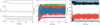 |
Fig. 4 Same as Fig. 3 but for the resonance sequence 3:2, 2:1, and 2:1. |
| In the text | |
|
Fig. 5 Random resonant solutions in the semimajor axis and eccentricity planet for the two different chains (3:2, 2:1, and 3:2 on the left and 3:2, 2:1, and 2:1 on the right). The solutions are scalable in semimajor axes, and the three inner planet semimajor axes can be shifted until they coincide with the observed ones. |
| In the text | |
|
Fig. 6 Evolution of the critical argument of the outer planet pair (b and e) initially locked in a 3:2 resonance. In the upper panel, the additional planet has a mass m = 200 M⊕, a = 8 au, e = 0.95, and i = 10°. In the bottom panel, a more massive planet on a less eccentric orbit was adopted (m = 2 MJ, a = 4 au, e = 0.85, and inclination i = 2°). In both cases, after a period of chaotic evolution, the onset of repeated close encounters breaks the resonance lock and leads to fast instability. |
| In the text | |
|
Fig. 7 SPHERE image of Vl298Tau in the H2 band with the faint background object at 2.77″ highlighted with the red arrow. |
| In the text | |
|
Fig. 8 Relative astrometric position of the proposed companion in the first and the last observing epoch. The solid black line represents the expected course of the companion if it were a stationary background object. The black square at the end of the line represents the expected position at the epoch of the last observation in this case. The minor difference between the observed and expected positions is consistent at ~1.5cr with measurement errors or could be due to a non-zero intrinsic motion of the background source. |
| In the text | |
|
Fig. 9 Mass detection limits (5σ) obtained from the SPHERE data (both IRDIS and IFS) expressed in units of Jovian mass as a function of the separation expressed in astronomical units. |
| In the text | |
|
Fig. 10 Gaia DR3 sensitivity to companions of a given mass (in units of Jovian mass) as a function of the orbital period (in years). Solid, dashed, and dashed-dotted lines correspond to iso-probability curves for 50%, 90%, and 99% probability of a companion of given properties to produce a RUWE value that exceeds the value reported in the Gaia DR3 archive (1.035). |
| In the text | |
|
Fig. 11 Detection function map of the RV time series of V1298 Tau from Suárez Mascareño et al. (2022), with the stellar activity already removed (i.e., the optimistic case). The color scale expresses the detection function, while the red dashed lines correspond to the 90% detection threshold including the stellar activity in the modeling (i.e., the pessimistic case). The blue circles correspond to the position of the measured planets in the systems, while the blue lines mark the upper limits of the planets with no mass-measurement yet. The left panel shows the Bayesian detection map computed for P < 400 days, while the right panel shows the inject-recovery detection map computed for 400 < P < 4000 days. |
| In the text | |
Current usage metrics show cumulative count of Article Views (full-text article views including HTML views, PDF and ePub downloads, according to the available data) and Abstracts Views on Vision4Press platform.
Data correspond to usage on the plateform after 2015. The current usage metrics is available 48-96 hours after online publication and is updated daily on week days.
Initial download of the metrics may take a while.