| Issue |
A&A
Volume 678, October 2023
|
|
|---|---|---|
| Article Number | A151 | |
| Number of page(s) | 29 | |
| Section | Catalogs and data | |
| DOI | https://doi.org/10.1051/0004-6361/202347333 | |
| Published online | 18 October 2023 | |
The LOFAR Two-Metre Sky Survey
VI. Optical identifications for the second data release★
1
Centre for Astrophysics Research, University of Hertfordshire,
College Lane,
Hatfield
AL10 9AB, UK
e-mail: This email address is being protected from spambots. You need JavaScript enabled to view it.
2
Cavendish Astrophysics, University of Cambridge, Cavendish Laboratory,
JJ Thomson Avenue
Cambridge
CB3 0HE, UK
3
SKA Observatory, Jodrell Bank, Lower Withington,
Macclesfield
SK11 9FT, UK
4
Institute for Astronomy, University of Edinburgh, Royal Observatory,
Blackford Hill,
Edinburgh
EH9 3HJ, UK
5
School of Physical Sciences, The Open University,
Walton Hall,
Milton Keynes
MK7 6AA, UK
6
Leiden Observatory, Leiden University,
PO Box 9513,
2300 RA
Leiden, The Netherlands
7
ASTRON, the Netherlands Institute for Radio Astronomy,
Postbus 2,
7990 AA
Dwingeloo, The Netherlands
8
Astronomical Observatory of the Jagiellonian University,
ul. Orla 171,
30-244
Krakow, Poland
9
Universidad Nacional Autonoma de Mexico (UNAM),
Avenida Insurgentes Sur 3000,
Mexico City, Mexico
10
Thüringer Landessternwarte,
Sternwarte 5,
07778
Tautenburg, Germany
11
Fakultät für Physik, Universität Bielefeld,
Postfach 100131,
33501
Bielefeld, Germany
12
INAF-IAPS,
Via Fosso del Cavaliere 100,
00133
Rome, Italy
13
Centre for Extragalactic Astronomy, Department of Physics, Durham University,
Durham
DH1 3LE, UK
14
Institute of Astronomy, Faculty of Physics, Astronomy and Informatics, NCU,
Grudziadzka 5,
87-100
Toruń, Poland
15
Space Radio-Diagnostics Research Centre, University of Warmia and Mazury,
ul.Oczapowskiego 2,
10-719
Olsztyn, Poland
16
INAF-Istituto di Radioastronomia,
Via P. Gobetti 101,
40129
Bologna, Italy
17
Hamburger Sternwarte, Universität Hamburg,
Gojenbergsweg 112,
21029,
Hamburg, Germany
18
Key Laboratory for Research in Galaxies and Cosmology, Shanghai Astronomical Observatory, Chinese Academy of Sciences,
80 Nandan Road,
Shanghai
200030, PR China
19
Department of Physics, Lancaster University,
Lancaster
LA1 4YB, UK
20
CSIRO Space and Astronomy, ATNF,
PO Box 1130,
Bentley, WA
6102, Australia
21
Departamento de Fisica de la Tierra y Astrofisica, Universidad Complutense de Madrid,
28040
Madrid, Spain
22
Department of Astronomy, Tsinghua University,
Beijing
100084, PR China
23
Inter-University Institute for Data Intensive Astronomy, Department of Astronomy, University of Cape Town,
7701 Rondebosch,
Cape Town, South Africa
24
Inter-University Institute for Data Intensive Astronomy, Department of Physics and Astronomy, University of the Western Cape,
7535 Bellville,
Cape Town, South Africa
25
Citizen scientist
Received:
1
July
2023
Accepted:
29
August
2023
Abstract
The second data release of the LOFAR Two-Metre Sky Survey (LoTSS) covers 27% of the northern sky, with a total area of ~5700 deg1. The high angular resolution of LOFAR with Dutch baselines (6 arcsec) allows us to carry out optical identifications of a large fraction of the detected radio sources without further radio followup; however, the process is made more challenging by the many extended radio sources found in LOFAR images as a result of its excellent sensitivity to extended structure. In this paper we present source associations and identifications for sources in the second data release based on optical and near-infrared data, using a combination of a likelihood-ratio cross-match method developed for our first data release, our citizen science project Radio Galaxy Zoo: LOFAR, and new approaches to algorithmic optical identification, together with extensive visual inspection by astronomers. We also present spectroscopic or photometric redshifts for a large fraction of the optical identifications. In total 4 116 934 radio sources lie in the area with good optical data, of which 85% have an optical or infrared identification and 58% have a good redshift estimate. We demonstrate the quality of the dataset by comparing it with earlier optically identified radio surveys. This is by far the largest ever optically identified radio catalogue, and will permit robust statistical studies of star-forming and radio-loud active galaxies.
Key words: catalogs / radio continuum: galaxies
The catalogues described in this paper are available at the CDS via anonymous ftp to cdsarc.cds.unistra.fr (130.79.128.5) or via https://cdsarc.cds.unistra.fr/viz-bin/cat/J/A+A/678/A151 and via the LOFAR surveys project website at https://lofar-surveys.org/dr2_release.html
© The Authors 2023
 Open Access article, published by EDP Sciences, under the terms of the Creative Commons Attribution License (https://creativecommons.org/licenses/by/4.0), which permits unrestricted use, distribution, and reproduction in any medium, provided the original work is properly cited.
This article is published in open access under the Subscribe to Open model. This email address is being protected from spambots. You need JavaScript enabled to view it. to support open access publication.
1 Introduction
The LOFAR Two-Metre Sky Survey1 (LoTSS; Shimwell et al. 2017) aims to survey the entire northern sky using the Low-Frequency Array (LOFAR; van Haarlem et al. 2013) at a central frequency of 144 MHz. The survey, which already covers a significant amount of the extragalactic northern sky, will provide an unrivalled resource for wide-area low-frequency selection of extragalactic samples, both of star-forming galaxies (hereafter SFG) and of radio-loud active galactic nuclei (hereafter RLAGN). In addition to the wide-field component, LoTSS has several deep fields with published and publicly available images and catalogues, including the Lockman Hole, Boötes (Tasse et al. 2021), and ELAIS-N1 (Sabater et al. 2021) fields. There is also a counterpart survey at lower LOFAR frequencies, the LOFAR Low-Band Antenna Sky Survey (LoLSS; de Gasperin et al. 2021). Key to the science goals of the project is accurate redshift information for the host galaxies of the radio sources. This information will be provided in part by more than one million optical spectra that will be obtained using the William Herschel Telescope Enhanced Area Velocity Explorer (WEAVE) instrument (Jin et al. 2023) as part of the WEAVE-LOFAR project (Smith et al. 2016), by the Sloan Digital Sky Survey (Blanton et al. 2017) and other ongoing and future large-scale spectroscopic campaigns such as the Dark Energy Spectroscopic Instrument (DESI; Levi et al. 2013) or the Euclid Wide Survey (Euclid Collaboration 2022), and for the remaining LOFAR sources by state-of-the-art photometric redshifts already in hand (Duncan et al. 2021).
In order to exploit the full potential of deep extragalactic radio surveys, we need optical identifications, and the photometric and/or spectroscopic redshifts that they make possible. Spectroscopic followup projects such as WEAVE-LOFAR also rely, where possible, on accurate optical positions of target sources. Historically, radio continuum surveys have produced catalogues of radio sources for others to follow up with further radio or optical observations: for example, the highly influential revised Third Cambridge Revised (3CR) sample of the brightest extragalactic low-frequency radio sources in the northern sky (3CRR; Laing et al. 1983), itself based on radio data taken in the 1960s (Bennett 1962; Gower et al. 1967), only received its final optical identification in 1996 (Rawlings et al. 1996). The radio survey that was the largest in terms of numbers of sources detected until very recently, the NRAO Very Large Array (VLA) Sky Survey (NVSS; Condon et al. 1998), which covers the whole sky above declination −40°, has never had anything approaching a full optical identification catalogue, partly because of the lack of any appropriate counterpart optical catalogue but also because its low resolution (45 arcsec) precludes reliable matching of the radio sources with deep optical data. Higher-resolution large-area surveys, such as Faint Images of the Radio Sky at Twenty-Centimeters (FIRST; Becker et al. 1995) are more easily matched to optical data, but high-resolution surveys with the VLA are insensitive to large-scale structure due to a lack of short interferometric baselines2, and so obtaining a catalogue that is both optically identified and flux-complete in the radio has historically involved labour-intensive combination of multiple radio catalogues with the optical data (e.g. Gendre & Wall 2008; Best & Heckman 2012). While the VLA Sky Survey (VLASS: Lacy et al. 2020), now in progress, will have excellent angular resolution and improved image fidelity compared to FIRST, it will still be insensitive to structures on scales larger than 30 arcsec.
A major complication of the process of optical identification of radio sources is due to the fact that radio structures, if properly imaged, can be physically large, with complex, resolved structure extending to much larger scales than those of the host galaxy observed in the optical. In extreme (but far from uncommon) cases, the catalogued positions of the two lobes of a double RLAGN may both lie arcminutes away from the true optical host and from each other (e.g. Oei et al. 2023). In situations like this two operations are required - the radio components must be ‘associated’, that is they must be recognised as a single physical source, and the source must be ‘identified’, that is an optical counterpart must be found. In general it is easier to do these two operations together and, at present, visual inspection remains the best way of doing so – a human being with a small amount of training can efficiently pick out radio structures that look like an extended radio galaxy and simultaneously select the best optical counterpart for the candidate radio source. For the very large surveys being generated by the current generation of radio telescopes, though, visual inspection is extremely expensive in terms of time. Banfield et al. (2015) describe ‘Radio Galaxy Zoo’, the first citizen-science project to aim specifically at providing associations and optical identifications for extended radio sources. Radio Galaxy Zoo involved the inspection by citizen scientists of ~100 000 radio sources, mostly from FIRST, and obtained infrared (IR) IDs from the Wide-field Infrared Survey Explorer (WISE) catalogue for a large fraction of them (56% in Data Release (DR) 1: Wong et al., in prep.), demonstrating the applicability of citizen science methods to such very large datasets.
The LoTSS surveys, because of the wide range of baselines provided by even the Dutch subset of LOFAR antennas, have the capability to detect extended emission on scales up to ~1° while also having resolution good enough (6 arcsec) for unambiguous identification of a large fraction of the detected radio sources and sensitivity nearly an order of magnitude higher than FIRST for sources of typical radio spectra, α ~ 0.7. It has always been the goal of the LoTSS project not only to produce the surveys, but also to provide the ancillary data needed for their scientific exploitation. In the first LoTSS data release, DR1, which covered 424 deg2 in a region of the Northern sky matched to the coverage of the Hobby-Eberly Telescope Dark Energy Experiment (HETDEX; Gebhardt et al. 2021), we were able to generate an optically identified catalogue (Williams et al. 2019) by combining the LoTSS data with Panoramic Survey Telescope and Rapid Response System (PanSTARRS) DR1 (Chambers et al. 2016) and AllWISE data (Wright et al. 2010; Mainzer et al. 2011), a process that generated a value-added catalogue of 318 520 radio sources, with plausible optical and/or IR counterparts for 73% of them. We developed an algorithm for deciding whether a particular radio source needed visual inspection for association and identification, described in detail by Williams et al. (2019). When required, we used a private Zooniverse project, ‘LOFAR Galaxy Zoo’ (hereafter LGZ), based on the approach of Radio Galaxy Zoo (RGZ), as a platform for distributing and collating the effort of inspection. This visual classification was largely done by members of the Surveys Key Science Project. The resulting optical identifications enabled a range of science including the study of RLAGN (Sabater et al. 2019; Hardcastle et al. 2019; Mingo et al. 2019), their environments (Croston et al. 2019) and their host galaxies (Zheng et al. 2020), giant radio galaxies (Dabhade et al. 2020), quasars (Gürkan et al. 2019; Morabito et al. 2019; Rankine et al. 2021), star-forming galaxies (Wang et al. 2019), and the search for extra-terrestrial intelligence (Chen & Garrett 2021). The process that we developed for DR1 was adapted to provide the optical identifications for the first release of the LoTSS deep fields (Kondapally et al. 2021), where an identification rate close to 100% was achieved thanks to the excellent optical data available in those fields.
The second wide-area data release, DR2, of LoTSS (Shimwell et al. 2022) covers 27% of the northern sky, but specifically targets areas at high Galactic latitude with good optical coverage for extragalactic sources. It has a total sky coverage of 5700 deg2, provided by 841 LOFAR pointings, and is split between two regions: the RA-13 (‘Spring’) region centred at approximately 12h45m00s +44°30′00″ and the RA-1 (‘Fall’) region centred at 1h00m00s +28°00′00″. The DR2 sky coverage (Fig. 1) reflects the contiguous sky area that the survey had built up at the start of the DR2 processing run in 2019, but excludes both the Galactic plane and also low-declination regions where the sensitivity of LOFAR is reduced due to geometrical effects; in total DR2 covers 46% of the extragalactic Northern sky with |b| > 10° and δ > 15°. DR2 contains 4.4 million catalogued sources, the largest radio source catalogue released so far, and so the required effort for optical identification and source association was over an order of magnitude larger than for DR1. We took an early decision to involve citizen scientists in the optical identifications for DR2 through a successor project to Radio Galaxy Zoo, which we named Radio Galaxy Zoo: LOFAR. For the remainder of this paper, this public project is referred to as RGZ(L) to make clear the distinction between it, the original RGZ, and our previous internal platform, LGZ.
In this paper, we describe the process of deriving optical identifications for LoTSS DR2 targets. Section 2 describes the datasets that we use for the optical counterpart catalogue and Sect. 3 describes the approach to likelihood-ratio cross-matching that we adopt for these datasets. Section 4 describes the choices made to decide whether likelihood-ratio matches should be used for a given source or whether visual inspection is needed for optical identification and/or association. Section 5 describes our public Zooniverse project, ‘Radio Galaxy Zoo: LOFAR’ and its outputs. We discuss the post-processing of the Zooniverse and likelihood-ratio identifications and associations in Sect. 6, source angular sizes are discussed in Sect. 7, and our methods for estimating photometric redshifts, galaxy masses and other physical quantities are briefly summarized in Sect. 8. The final catalogue is described in Sect. 9. We discuss some properties of the sources in the resulting catalogue in Sect. 10 and summarize our results in Sect. 11.
Throughout this paper we use a cosmology in which H0 = 70 km s−1 Mpc−1, Ωm = 0.3, and ΩΛ = 0.7. Radio flux density is quoted in Jy: 1 Jy is 10−26 W Hz−1 m−2. The radio spectral index α is defined in the sense Sν ∝ ν−α. Optical and IR magnitudes used are in the AB system unless stated otherwise. Code used for the operations described in this paper is available for download and modification online3.
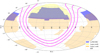 |
Fig. 1 Sky coverage of the LoTSS DR2 (blue) and the Legacy DR9 (yellow and orange) optical surveys. The purple lines (‘MW’) show the Galactic plane and lines of |b| = 10°. As described in the text, ‘Legacy North’ data is made up of BASS and MzLS data, ‘Legacy South’ data are from DECaLS. |
2 The input data
For radio data, our starting point is the DR2 images and combined catalogue described by Shimwell et al. (2022). The images used are the mosaiced images described in that paper, which have the greatest depth at any position in DR2. The catalogue is a radio catalogue generated by combining runs of the Python Blob Detector and Source Finder (PYBDSF; Mohan & Rafferty 2015) over all the mosaics, and so is the result of decomposing the image of the sky into many Gaussian components. For our purposes the key elements of the catalogue are, for each source: position, total flux density, major and minor full width at half-maximum (FWHM) and position angle of the fitted Gaussian, and the deconvolved versions of the last three quantities (i.e. after correcting for the 6-arcsec restoring beam). For the cataloguing parameters that we use, PYBDSF can sometimes combine the originally detected Gaussians into composite sources, and so for some purposes (discussed further below) we use the original Gaussian catalogue as well as the DR2 source catalogue. Since the latter is the starting point for our later efforts to associate components together into sources, we refer to it as the component catalogue in what follows.
Optical data for the identification effort are provided by the DESI Legacy Imaging Surveys, hereafter the Legacy Survey4 (Dey et al. 2019). This combines three optical surveys of the sky away from the Galactic plane: the Dark Energy Camera Legacy Survey (DECaLS), covering mostly southern declinations, and the Beijing-Arizona Sky Survey (BASS) and Mayall z-band Legacy Survey (MzLS), covering the northern sky. The coverage of the Legacy survey is shown in relation to LoTSS DR2 in Fig. 1. As can be seen in that figure, the bulk of our sky coverage in the RA-13 region is from BASS and MzLS, which reach typical point-source depths of 24.3, 23.7, and 23.3 mag in the g, r and z bands respectively. The coverage available in the RA-1 region, and a small amount to the south of the RA-13 region, is from the deeper DeCALS which reaches mean depths of 24.8, 24.2, and 23.3 mag in the northern sky, with the extinction-corrected depth being more or less constant over the areas of interest to LOFAR. Even the northern parts of the survey are 1.0 mag deeper in g and z, and 0.5 mag deeper in r, than PanSTARRS DR1, which provided the optical data for our DR1 optical cross-matching effort.
As can be seen in Fig. 1, there is an area of DR2 to the north of the RA-1 field that does not have Legacy Survey coverage, amounting to 48 LOFAR pointings or a little over 300 deg2 of our area. For simplicity this area is omitted from our analysis and from the value-added catalogues, which reduces the number of radio sources that can be optically identified to ~4.1 million.
For our likelihood-ratio cross-matching, as discussed below, we combined the Legacy DR9 ‘sweep’ catalogues, joining North and South at a declination of 32.375°. To obtain FITS images for visual inspection (Sects. 5 and 6) we used the publicly available survey web-based APIs to download WISE band 1 and grz Legacy image cubes. Around 2600 4096 × 4096 WISE images and 295 000 1000 × 1000 × 3 Legacy cubes, totalling ~3 TB, were downloaded.
3 Likelihood-ratio cross-matching
We cross-matched radio sources to their optical and/or IR counterparts using a likelihood-ratio (LR) method (Sutherland & Saunders 1992). First, we cross-matched the Legacy Survey data with the unWISE data (Schlafly et al. 2019) to create a combined optical and IR catalogue. We used a simple nearest neighbour match limited to a maximum radius of 2.0 arcsec to match optical to IR sources. This value for the radius was empirically found to be optimal to provide actual matches. Unmatched sources were added to the final combined catalogue without corresponding WISE or Legacy photometry. The combined optical and IR catalogue was then cross-matched to the LoTSS DR2 radio sources using the LR method presented by Williams et al. (2019), which uses both optical magnitude and colour as an input. This LR method is a statistical technique to match counterparts of the same source observed at different wavelengths. We considered ten colour (r-band to unWISE W1) bins plus two bins for objects with only unWISE data: one for objects with W1 and W2 magnitudes, and one for objects with only W2 magnitudes.
The cross-match was done separately for three different regions: a) the RA-1 (‘Fall’) region which is covered by the Legacy South survey; b) the RA-13 (‘Spring’) region covered by the Legacy South survey; and, c) the RA-13 (‘Spring’) region covered by the Legacy North survey. We did this to take into account the different locations on the sky and the possible differences in the optical survey properties. Within each of these regions we computed the Q0 values (where, as described by Williams et al. 2019, Q0 represents the fraction of sources that have an optical counterpart down to the magnitude limit of the survey) in different areas where the optical and IR coverage was complete. The values of Q0 for those different areas within a region were similar within the errors. This suggests that the range of declinations did not generate any significant biases for the LR method. The LR cutoff thresholds for the different regions are slightly different for the different regions, as expected. As a result of the LR matching, every source either had a bestmatch LR candidate ID, or no potential counterpart above the LR threshold.
4 The decision tree
The decision tree used for selecting which radio sources to accept their statistical LR identification (or lack thereof, see Sect. 3) and which sources to further process visually through the public RGZ(L) Zooniverse project (described in Sect. 5) was very similar to that used by Williams et al. (2019) for LoTSS DR1. This decision tree aims to identify ~~PYBDSF~~~ sources that are components of physical radio sources and that therefore need to be associated before the optical and IR cross-identification is made, together with other sources that are not suitable targets for the LR method. Here we give only a brief summary and highlight any changes to the process used for DR1. Figure 2 shows the modified decision tree used in this work, along with the numbers and fractions of sources at each outcome. Key parameters used for the decisions are defined in Table 1. A separate decision process is followed within the decision tree for ~~PYBDSF~~~ sources that are composed of multiple Gaussians. The decision tree used for this was essentially identical to that used for DR1 and is described by Williams et al. (2019).
The input parameters to the decision tree are the ~~PYBDSF~~~ source size (taken to be the major axis), source flux density, and number of fitted Gaussian components, as well as the calculated distances to the nearest neighbour (NN) and to the fourth closest neighbour (NN4). Further inputs are the likelihood ratios for sources smaller than 30 arcsec as well as for individual Gaussian components smaller than 30 arcsec. The outcomes of the decision tree are labels for each ~~PYBDSF~~~ source which determine how it should be treated subsequently. Some of these are derived directly from the source properties, but, as for DR1, some outputs of the decision tree required ‘visual sorting’ or filtering done by a small number of experienced people. This rapid process, performed using a simple P~~YTHON~~~ interface to view the RGZ(L) images and categorise the sources, was done to avoid overpop-ulating the RGZ(L) sample with sources that would not benefit from citizen science inspection.
A key difference with the DR1 flowchart was that we did not attempt to include faint sources, below a total flux density of 4 mJy, in the list of objects sent to RGZ(L) for visual sorting. The reason for this was twofold: firstly, experience from DR1 shows that these faint objects are often extremely difficult to associate and identify, especially for large sources; secondly, these sources are very numerous and would overwhelm the capacity of the Zooniverse project. The level of the limit was selected because we were aiming to produce an almost complete sample of physical radio sources for the WEAVE-LOFAR project, which will target all LoTSS sources brighter than 8 mJy for spectroscopic followup. In almost all cases we used a limit of 4 mJy, as these ~~PYBDSF~~~ sources might be components of an 8-mJy physical source and need to be associated, thereby ensuring greater completeness for the WEAVE 8-mJy flux-density selection criterion. Only in the branch of the decision tree addressing small, isolated, multiple-Gaussian component sources did we use a different limit of 8 mJy since, given their isolation, these sources are unlikely to be components of another source. Within this category of faint sources, all except the largest sources (>15 arcsec) will have LR determinations available, and the identification (or lack thereof) from these has been adopted for the catalogue; these can be used with the caveat that they may be wrong if the source is actually a component of a larger physical radio source. However, Williams et al. (2019) showed that not many sources in this flux range benefited from visual inspection.
A second key change to the decision tree from DR1 was the inclusion of the machine-learning (ML) classifications developed by Alegre et al. (2022). This gradient-booster classifier, whose features are similar to the parameters used in the decision tree here, was trained using the final outcomes from the DR1 processing, that is, whether a ~~PYBDSF~~~ source needed to be associated or deblended or had a different identification to that provided by LR, and therefore needed to be processed with LGZ, and used to predict the same for the DR2 ~~PYBDSF~~~ sources. While these ML classifications were not used to fully replace the decision tree, they were used to reduce the number of sources requiring visual sorting in several branches of the decision tree. Firstly, for large (>15 arcsec) and intermediate flux density sources (4 < S < 8 mJy), instead of visually sorting all sources, we used the ML classifications to select most (95%) for direct processing in RGZ(L), while only the remaining 5% were visually sorted. Roughly half of the latter category were selected for RGZ(L) after the visual inspection process. Secondly, the ML classifications were also used for clustered sources. Faint sources (< 4mJy) were not processed, while the brighter sources with ML RGZ(l) classifications were processed directly in RGZ(L) and the remainder through visual sorting. Finally, the non-isolated sources without LR identifications that did not meet either the flux density or separation criteria to identify possible double sources were selected either for RGZ(L) or visual sorting based on the ML classification after excluding the faintest (< 4mJy) sources. We are confident that this ML approach did not prevent unusual sources from being inspected through the RGZ(L) platform, as (a) the training data from DR1 are very well matched to the type of data used in DR2 and (b) the training set size from DR1 was close to 10% of the total size of DR2, meaning that all source types seen in DR2 are likely to be well represented in the training set.
The final outputs of the decision tree, combining algorithmic, machine-learning, and visual inspection outcomes, are flags indicating which of several post-processing steps are required. These outcomes are summarized in Table 2 along with the number of PYBDSF sources within each category. Similar to the approach of Williams et al. (2019), the visual sorting used in several branches of the decision tree identifies some sources directly for the post processing which is normally applied to sources that have passed through the RGZ(L) project, either through the deblending or too-zoomed-in workflows (described in Sect. 5).
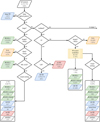 |
Fig. 2 Representation of the decision tree used to process all entries in the PYBDSF catalogue lying in the Legacy Survey sky area. Following this workflow a decision is made for each source whether to: (i) make the optical and IR identification, or lack thereof, through the LR method (blue and red outcomes respectively); (ii) process the source in RGZ(L) (green outcomes, including direct RGZ(L) post-processing); (iii) reject the source as an artefact (grey outcomes). The key parameters are defined in Table 1. The number and percentage of PYBDSF sources in each final bin are shown for each final outcome. Some faint sources are not processed further (orange outcomes); these are discussed in the text. |
Summary of the decision tree outcomes.
5 Zooniverse visual inspection
Almost all of the objects selected above as requiring visual inspection were sent to citizen scientists5 participating in the RGZ(L) project through the Zooniverse web interface6. The basic process for generating these images was very similar to that described by Williams et al. (2019), with radio and optical images again being generated using ~~APLPY~~~, but was modified to present citizen scientists with a simpler and more attractive view of the targets. Figure 3 shows an example of the three views provided to Zooniverse volunteers for one randomly chosen LOFAR source from the ‘large, bright’ category, where the user can flip between all three views at any time. The main differences in this interface compared to the LGZ interface used for DR1 was the inclusion of a multi-colour optical image, a colourmap version of the radio image (to enhance accessibility), and the exclusion of the WISE image. The latter choice was made to simplify the interface at the cost of losing a small number of distant RLAGN which are easy to spot in near-IR, since many of those sources were recoverable using the steps described below.
The field of view presented to the user for each catalogued radio source was chosen algorithmically with the aim of maximizing the probability of seeing all of a large, multi-component source. Initially the field of view was taken to encompass all of the target source itself, where a catalogued component from the DR2 catalogue with deconvolved FWHM values θmaj and θmin is represented by an ellipse with semi-major axis θmaj and semi-minor axis θmin. It was then extended iteratively to cover any other overlapping elliptical components; this helps to ensure that complex contiguous sources, where possible, are represented in the image sent to Zooniverse. Next, nearby resolved neighbour objects from the component catalogue with total flux density similar to (no more than a factor three less than) the target source and an offset of no more than 3 arcmin from the field centre were iteratively added to the field of view - once a nearest neighbour was added, the mean positional centroid of all the sources selected so far was calculated and the process repeated until convergence. This approach was intended to pick up, for example, lobes of a double source that might have similar total flux density but did not appear to overlap on the sky. Finally, the centroid and bounding box of the resulting set of components were computed. If the bounding box was larger than 5 arcmin, then only the size of the original component was used. This prevented very large fields being sent for inspection, as those would present the user with too large a field of view to reliably select components and optical counterparts. A minimum field of view of 1 arcmin (ten times the FWHM of the LOFAR restoring beam) was also imposed to ensure that at least some neighbouring sources and galaxies would be visible. Finally, the field of view used was rounded to the nearest 10 arcsec (this allows for simple formatting of the number when the data are uploaded to Zooniverse in ASCII format) and the three images were generated. As illustrated in Fig. 3, ellipses mark the positions of all catalogued radio sources in the field of view, with a solid ellipse indicating the ‘current’ source and dashed ellipses indicating others that might potentially be associated with it.
Citizen scientists were asked to go through a three-stage process for each source sent to Zooniverse, illustrated in Fig. 4. These can be summarized as ‘association’, ‘identification’, and ‘commenting’. In the first step, volunteers were asked to select any radio sources in the field of view that were physically associated with the object of interest (indicated with a solid ellipse) by clicking on the image. Next, they were asked to select one or more potential optical identifications for the associated source in the same way. In the final screen they could select one or more flags to indicate potential problems with the source, and/or choose to leave comments on the object on the Zooniverse talk page. Problems that could be flagged up included stating that the source was an artefact (i.e. not a physical source), that the source combined emission from two or more separate sources (a blend), that it was too zoomed in (i.e. there might be associated components outside the field of view), that one or other of the required images was missing, or some other general problem with the image (for example a bright star preventing the optical identification). Volunteers were also encouraged to tag the objects with descriptive but consistently used words (‘hashtags’: cf. Rudnick 2021) which could be recovered in processing. No previously defined hashtags were supplied, so the consistent use of these relied on communication between participants on the Zooniverse forums.
To guide and train the citizen scientists in the process, various resources were made available. The first time a user started classifying, a text-based tutorial appeared on the screen which explained the interface, the radio-optical overlay and the association, identification and commenting tasks. Additionally, we provided a tutorial video which explained the process with ten examples of common radio sources. Finally, a separate interactive training workflow was set up where volunteers could practice on those ten example radio sources and receive feedback interactively after clicking on the images. The project and text based tutorials were made available in eight languages7, while the tutorial video was made in four different languages, plus an additional version using closed captions.
Following the approach of Williams et al. (2019), we required a minimum of five classifications for each catalogued source, but large complex physical sources are often broken down into smaller sub-components in PYBDSF, so that many more individual classifications can contribute to the interpretation of a complex source. A refinement added part-way through the process was to ‘retire’ after only three views a source that no user had classified in any way at that point. This avoids wasting user time on sources where volunteers have nothing to say (i.e. compact sources with no optical identifications).
A total of 189 375 sources (4% of the total source count in the survey) were sent to RGZ(L): this includes 104582 large, bright sources (where we selected sources with flux density > 8mJy and size >15 arcsec but also a peak flux >2 times the local rms noise)8, 64835 sources with flux density >4 mJy selected directly from decision tree endpoints, and 19 958 sources prefiltered from decision tree endpoints by visual inspection from members of the project team. Results from RGZ(L) were initially processed in the manner described by Williams et al. (2019). User ‘clicks’ were provided in the JSON-format Zooniverse output, and these were matched to the radio and optical and WISE catalogues. Once clicks had been matched to the catalogue, quality factors for the association and identification of the sources were calculated based purely on the fraction of Zooniverse volunteers who had picked any particular identification or association. Overall, the whole process differed from the approach taken with our internal LGZ platform used for DR1 only because we used a magnitude-size relation for galaxies to give more leeway to the optical identifications with bright, nearby, extended galaxies. The default maximum circular offset threshold was 3 arcsec but it could be extended up to ~25 arcsec for the brightest galaxies.
A total of 957 374 classifications were made through the Zooniverse system by 13 711 distinct users, including users who were not logged in to the platform. Of these, only ~100 made more than 1000 classifications - the most prolific ~125 volunteers contributed half the total classifications. The distribution of user classification numbers is plotted in Fig. 5. It can be seen that several thousand volunteers tried classifying just once or twice before disengaging with the project – this may be a reflection of the comparative difficulty of the combined radio and optical classifications. However, the numbers level off above a few tens of classifications and show a rough power-law form between 100 and ~2000 classifications. This type of distribution is not uncommon, in some parts of the range, for measures of ‘scientific productivity’, loosely defined (Lotka 1926). For projects like this one it means that many of the classifications will be contributed by volunteers who have had the opportunity to develop expertise in source classification. Volunteers with more than 2000 classifications were offered co-authorship on this paper and personally contacted for assistance in finishing off the later parts of the project, and this may account for the change in the slope of the histogram at this point.
Interestingly, the raw rate of optical identification from the Zooniverse project was low. Only 27% of all sources sent to be viewed by volunteers returned with a consensus optical ID (that is, one where more than 2/3 of the votes on a given target agreed on the best associated optical object: examples of sources where this is and is not the case are shown in Fig. 6). This contrasts with 51% for the internal classifications through the same interface, and illustrates the difficulty of selecting the right optical object for relatively untrained volunteers. By contrast, the fraction of radio sources associated with others (around 18%) is similar for astronomers and Zooniverse volunteers as a whole. Objects with no consensus optical ID may still have associations and simply propagate through to the next stages of processing with no ID. On visual inspection of a randomly selected subsample of the RGZ(L) optical IDs by two independent astronomers, the error rate was found to be ~3%; in other words, the RGZ(L) optical ID process is conservative and probably does not assign an ID to every source that should have one, but where an ID is assigned, it is almost always correct.
As we have no ‘gold standard’ sources, we have no means of assessing the quality of individual volunteers’ classifications as objectively good or bad. What we can do instead is to assess the extent to which volunteers tend to agree with others. To do this, for optical IDs, we considered the final RGZ(L) source catalogue, and compared all optical ID classifications made by volunteers to it. If the final catalogue contained no ID for the source, each user who selected no ID for that particular source scored one point, and all volunteers who selected any ID scored no points. If the final catalogue did contain an optical ID, volunteers who had selected an ID positionally matched to the one in the catalogue scored one point, and all others scored no points. Dividing the points scored by the number of sources classified by each user gives a per-user ‘consensus score’ which must lie between 0 and 1, and the histogram of this (for all volunteers with more than 100 classifications, to give adequate statistics) is shown in Fig. 5. Since a selected optical ID requires more than 3/5 classifiers to agree on it, we expect this score to exceed 0.6 in general - that is, for any finally catalogued optical ID, at least 3/5 volunteers should score points. Consistent with this, the median of the consensus score is almost exactly 0.6. Volunteers who had a consensus score much lower than this were consistently disagreeing with other volunteers, and this suggests that they were not interpreting the images in the same way. Over 116 000 classifications were made by volunteers whose consensus score was less than 0.3. The histogram also shows that a few volunteers, generally with quite small numbers of classifications, have consensus scores approaching 1.0. Since this degree of consensus would be quite hard to achieve by other means, we suspect that these are volunteers who declined to classify (by hitting reload) all sources where the optical ID was not obvious, but this hypothesis cannot be confirmed from the available data on user interactions with the Zooniverse platform, which does not list classifications that were started but not completed.
Given the wide range of consensus scores for optical IDs and the low optical ID fraction, we elected to rerun the processing code with volunteers’ optical ID votes (only) reweighted by their consensus scores as shown in Fig. 5: volunteers who had not classified more than 100 objects were given a weighting of 0.6, the median value. This gave a modest improvement in the optical ID fraction from the RGZ(L) volunteers, increasing it to 31%, and so it is these consensus optical IDs which are fed to the next stages of the process.
Hashtags assigned by volunteers to each source were added to a supplementary catalogue file made available as a JSON dictionary. This will allow catalogue users to search easily for objects which have been tagged in a particular way. Widely used tags are listed in Table 3, and include a number which could give morphological information on the resulting source. However, it is worth noting that these tags were not consistently applied and should not be used to try to derive complete samples. Some morphological structures are labelled more reliably than others; for example, there are a reasonable amount of wide angle tailed sources labelled as WATs, but very few of the sources tagged as NATs have narrow angle tails, even though both tags have been applied a similar number of times. In general around 10–40% of tagged sources appear to be clearly described by their morphological tags. Additionally, only a small percentage of objects of any given kind were tagged to begin with.
 |
Fig. 3 Example of the three images presented to citizen scientists for one catalogued LOFAR radio source (ILTJ093236.46+602825.5). Left panel, the default view: radio contours from the LOFAR data (logarithmically increasing by a factor two at each interval from five times the local noise level) are superposed on the Legacy three-colour image. Cyan ellipses denote catalogued radio sources, with sizing as described in the text; the solid ellipse is the one under study and dotted ellipses represent other sources in the radio catalogue. Middle panel: the colour scale shows the LOFAR radio data only. Right panel: a view of the optical sky only. This image is 2 arcmin on a side. |
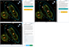 |
Fig. 4 Images from the classification section of the Zooniverse interface. This shows the three task screens presented for one catalogued source, ILTJ172125.82+370417.2, seen by the user in the order top left, top right, bottom left panels. The image shown here is 100 arcsec on a side. All three views here show the standard image (Legacy colour scale, radio contours, and ellipses to represent catalogued Gaussians). In the first panel, the marker for an associated component can be seen; in the second panel, the user has also marked an optical identification for the radio source. In the third panel, the user has the opportunity to apply various flags to the source or to discuss it on the talk pages. Note the unassociated radio source to the southeast (bottom left). The toolbar below the image allows the user to switch images, to get information on the source, to invert the colour map, or to add the source to a list of favourites. Additionally, the user has the option to zoom, pan, and rotate the image using the buttons on the right. |
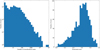 |
Fig. 5 Statistics of the Zooniverse volunteer population. Left: histogram showing the numbers of Zooniverse volunteers who made a certain number of classifications. On a log scale the rough power-law distribution of classification numbers is apparent, with a slope ≈ − 1. Right: histogram of the distribution of optical ID consensus scores for volunteers with more than 100 classifications. |
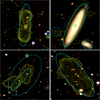 |
Fig. 6 Examples of RGZ(L) subjects with the optical and radio contour image seen by Zooniverse platform volunteers overplotted with the optical IDs selected by the volunteers, marked as green crosses. All sources have five or more optical ID selections (volunteers could optionally select more than one possible ID). The top row shows examples where a consensus was achieved and the correct optical ID selected, the bottom row ones where no consensus was found and no optical ID returned from RGZ(L). |
6 Catalogue generation, further visual inspection, and processing
Once the RGZ(L) outputs were processed, a first catalogue was created by merging the decision tree results (including a decision on whether or not to accept a likelihood-ratio optical ID for a given source) with the radio and optical catalogue generated by the process described in the previous section. For this we adapted the code written for the LoTSS Deep Fields analysis (Kondapally et al. 2021) which keeps track of the provenance of all finally generated sources, their components and their optical identifications. The output of this combination was (i) an initial catalogue of associated sources that combines the basic ~~PYBDSF~~~, optical, and RGZ(L) catalogues into one, along with provenance information, and (ii) a component catalogue that allows the final state of each PYBDSF source (whether as a catalogued source in its own right or as a component of an associated source) to be looked up. Objects flagged by a majority of Zooniverse volunteers as artefacts (or flagged as artefacts in the pre-filtering process discussed in the previous section) were removed from the catalogue at this point, and the catalogue generation process also generates derived table entries for quantities like the total flux density of a composite source from RGZ or the maximum size of the convex hull enclosing all of its components (Composite_Size).
Notes. Italics indicate tags that are descriptive of the images seen by the volunteers or the processes they followed rather than the sources themselves.
Further visual inspection was needed for a small minority of sources after this was done, with the aim being to ensure that the catalogue was as accurate as possible for extended, complex radio sources. This was done using six workflows carried out by astronomers on the LoTSS team, all of which involved an expert classifier editing either or both the association or identification of the catalogued source. These ran roughly in the following order:
‘First deblend’: in this workflow ~~PYBDSF~~~ components of a single composite source were broken down into their component Gaussians in order to allow a finer-grained allocation of radio sources to optical counterparts. This was particularly important in the case of two close but physically distinct radio sources that were merged into one ~~PYBDSF~~~ source. Sources flagged as blends by more than half of RGZ(L) volunteers or in pre-filtering were either sent to this workflow or to ‘Second deblend’ (see below). Users of the workflow could choose to send deblended sources on to the ‘too zoomed in’ workflow (see below) for further processing.
‘Too zoomed in’ (TZI): this workflow was used for sources where RGZ(L) volunteers flagged sources as ‘too zoomed in’ meaning that there appeared to be extended structure on scales larger than was visible in the image presented to the user. This was also used for sources prefiltered as TZI, or sent directly there by other workflows such as ‘Postfilter’ or ‘First deblend’, or for sources that exhibited other problems after the initial processing of the RGZ(L) catalogue. The original ~~PYBDSF~~~ component decomposition was retained and components could be added (or removed) from the current output of the catalogue to generate a new composite source. Remaining blended sources could be sent on to the ‘Second deblend’ workflow and the size of a source could be recorded manually if the PYBDSF components did not represent this well.
‘Deduplication’: this workflow provided a simple interface for merging objects with duplicate optical IDs or removing one of the duplicates as an artefact, and was set up part-way through the processing to reduce the labour costs of the more time-consuming TZI workflow. It was applied after the production of the initial catalogue.
‘Postfilter’: this workflow involved the visual inspection of all sources from the Zooniverse or TZI workflows with an angular size (Composite_Size) greater than 1 arcmin in order to check the validity of the source association - the ‘post-filtering’ step. Around 30% of these sources were flagged as problematic in some way (mostly sources that should have been flagged as ‘too zoomed in’ by RGZ(L) volunteers but were not) and these were sent on to a further iteration of the TZI workflow. A small number were flagged as blended and sent to the ‘Second deblend’ workflow.
‘Blend prefilter’: later in the processing, prefiltering was carried out on a large number of sources flagged as blends by RGZ(L) volunteers or by the flowchart to check whether these were genuine blends (which were sent on to the ‘Second deblend’ workflow) or should be dealt with in some other way, such as splitting into all individual components with IDs. This was an important step as only around 13% of blend prefiltered sources were sent to the time-consuming ‘Second deblend’ workflow.
‘Second deblend’: this workflow was a combination of TZI and deblending that allowed detailed editing of the components of complex sources, including the ability to include previously unassociated components, which was missing in ‘First deblend’. Sources flagged in Postfilter, TZI or (later in the processing) by RGZ(L) volunteers as blends were sent to this workflow, as shown in Fig. 7.
Finally, a version of the ridge-line optical ID code RL-XID of Barkus et al. (2022) was used on large (> 15 arcsec) sources with flux density above 10 mJy that did not have an optical ID assigned from visual inspection. This code, which uses the radio morphology of extended sources to help to select the most plausible host, allowed us to pick up a number of WISE-only or faint optical IDs that had been missed by RGZ(L) volunteers and/or by the expert classifiers. Relative to the version of the code described by Barkus et al. (2022), the main changes were optimizations of the size measurement and flood-filling algorithms to allow the code to run in reasonable time on the large number of sources present in DR2. The size and flux density limits were selected based on tests of the reliability of the ridge lines constructed by the code.
Table 4 gives the recorded radio source provenance, as recorded in the Created column, of all sources in the final catalogue, and the sources of optical IDs (Position_from) for all objects that have them. It can be seen that the vast majority of optical IDs (97%) come from the likelihood-ratio cross-matching (LR). However, Fig. 8 shows that half of all IDs for the brightest sources, and nearly 100% of IDs for the largest sources, come from visual inspection. The curves of optically identified fraction as a function of flux density and source largest angular size show that our methods are not uniformly good at identifying all sources: the fact that no source with a flux density less than 4 mJy was sent to visual inspection and only sources with fluxes > 10 mJy went to the ridge line code leads to a drop in the fraction of sources with IDs between 1 and 10 mJy, while the ID fraction steadily rises above this point. It is noteworthy that fewer than half of the sources returned from RGZ(L) have an ID returned from visual inspection, even after TZI processing. The sharp increase in the ID fraction above an angular size of 2 arcmin is presumably due to the postfilter step, and the data suggest that more IDs could be obtained with yet more visual inspection of sources with sizes >30 arcsec.
More details of the different routes to optical IDs are provided in the ID_flag column of the final catalogue, and the statistics of this are given in Table 5. At the end of the processing we achieved an 85.0% optical ID fraction for sources in the Legacy sky coverage.
Tags applied by RGZ(L) volunteers to 50 or more sources.
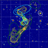 |
Fig. 7 Example user interface for the ‘Second deblend’ workflow. In an interactive Matplotlib window the expert classifier has separated the emission from two extended sources that had been combined in PYBDSF, seen in green and cyan, and has selected optical IDs for both. An unrelated source marked in white has been left unchanged. The new source is a mixture of PYBDSF components (solid lines) and Gaussians (dashed lines). |
Provenances of radio sources, IDs, redshifts, and sizes in the final catalogue.
Final ID flag statistics for sources with optical ID.
7 Radio source angular size estimates
As discussed above, non-composite sources have a size estimate (twice the deconvolved major axis of the fitted Gaussian), while a rough size estimate for composite sources can be obtained from the largest dimension of the convex hull encompassing all of the ~~PYBDSF~~~ components (Composite_Size). A small number of sources also have manual size measurements made during the too-zoomed-in visual inspection process. Because ~~PYBDSF~~~ tends systematically to overestimate the size of faint components (Boyce et al. 2023), while sometimes not detecting at all the largest-scale parts of an extended radio source, this size estimate is not ideal for physical size inference. As part of the L~~O~~~M~~ORPH~~~ (LM) code, Mingo et al. (2019) describe a method for estimating what we here refer to as ‘flood-fill sizes’, in which the ~~PYBDSF~~~ ellipses are used as the starting point for a measurement which in principle should include only the pixels of the image of the source that are above the local noise level. This method cannot return a size estimate much smaller than the beam size (i.e. the beam is not deconvolved from the size estimate) and so it is not suitable for application to compact sources.
We applied the flood-fill method to all sources in the catalogue with total flux density >5 mJy and estimated extended size >20 arcsec, 147 141 sources in total. The code returns flags if the flux density in the flood-fill source is significantly below the lower limit in the input catalogue, or if there are too few pixels to estimate a size after masking, and these, along with the size estimates, are included in the catalogue (column names LM_size, LM_flux, Bad_LM_flux and Bad_LM_image).
Some heuristic is then needed to make an overall best angular size estimate. The small number of manual size measurements in the catalogue (which can be assumed to be accurate since they are based on visual inspection) offer a guide: many of the flood-fill sizes are in good agreement with the manually measured sizes but some are smaller by a significant factor. The latter group, on inspection, are all sources with faint extended structure which does not appear above the noise floor in the flood-fill code. To some extent this problem can be mitigated by requiring the flux density measured by the flood-fill code to be close to the total catalogued flux density of the source - if a significant fraction of the radio emission is missing that can be taken as an indication that the flood-fill code is missing important structure.
To obtain an overall best size estimate (largest angular size, or LAS) we proceed as follows:
If a manual size measurement is available, we use that.
If not, a catalogue-based LAS is estimated by taking the Composite_size where available, and 2×DC_Maj otherwise.
The flood-fill size, if one exists, is adopted as the LAS in preference to the catalogue-based one if all three of the following conditions are met:
- (a)
No flood-fill flags are set
- (b)
The flood-fill flux density matches the catalogue flux density to within 20%
- (c)
The LAS is larger than 30 arcsec and smaller than 600 arcsec (this avoids regions where the flood-fill code cannot return good results).
- (a)
The final LAS and, for each source, an indication of the origin of the LAS (LAS_from) are given in columns in the final catalogue and the distribution of the origins of LAS is shown in Table 4. Sources where the LM_Size is adopted even though it is significantly different from the Composite_Size should be treated with caution - visual inspection shows that some of these sources have genuine low-surface brightness extended structure that was missed by the flood-fill algorithm, while others are point sources surrounded by artefacts.
For sources where the size estimate comes from the fitted Gaussian (the vast majority) we implement the resolution criterion of Shimwell et al. (2022), in the Resolved column of the catalogue. Size estimates should only be used where the source is flagged as resolved. All sources with alternative size measurements are taken to be resolved.
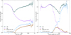 |
Fig. 8 Fractional optical IDs in the DR2 catalogue. The two plots show the total fraction of optically identified objects, and the breakdown by different methods of optical identification, as a function of (left) total flux density of the resulting source and (right) catalogued largest angular size. |
8 Redshifts and physical source properties
8.1 Spectroscopic and photometric redshifts
Photometric redshift (photo-z) estimates for the LoTSS sample with optical detections in the Legacy Surveys DR8 are taken from Duncan (2022), where full details of the methodology, training samples, and catalogue properties are presented. In summary, the photo-z estimation methodology was designed to produce robust photo-z predictions for a broad range of optical populations, including active galactic nuclei (AGN). The method employed Gaussian mixture models (GMMs) derived from the colour, magnitude, and size properties of the observed population to divide it into different regions of parameter space for training and prediction. The sparse Gaussian processes redshift code GPZ (Almosallam et al. 2016a,b) was then used to derive photo-z estimates for individual regions of observed parameter space, including cost-sensitive learning weights derived from the GMMs to mitigate against biases in the spectroscopic training sample.
Duncan (2022) explored the photo-z performance as a function of spectroscopic redshift, optical magnitude, and morphological type, finding that the photo-z estimates offer substantially improved reliability and precision at z > 1, with negligible loss in accuracy for brighter, resolved populations at z < 1 when compared to other photo-z predictions available in the literature for the same optical population. Crucially for the LoTSS sample, the photo-z predictions for the radio continuum selected population are suitable for use over a wide range in parameter space - with low robust scatter (σNMAD < 0.02–0.10) and outlier fraction (OLF015 < 10%)9 at z < 1 across a broad range of radio continuum (and X-ray) properties. At a given true redshift, zspec, there is no evidence that photo-z precision or reliability exhibits any dependence on the radio continuum flux density (and hence luminosity). The photo-z quality for a given LoTSS sample will therefore largely be dictated by the associated optical properties.
In the combined value-added catalogues presented in this paper we provide the derived photo-z columns presented in Table 3 of Duncan (2022). By construction, the GPZ predictions are unimodal, with zphot representing the mean of the normally distributed photo-z posterior and zphot_err the corresponding standard deviation.
In addition to the photo-z estimates, we also included spectroscopic redshifts from the Sloan Digital Sky Surveys Data Release 16 (SDSS DR16; Ahumada et al. 2020) when available. As the LoTSS DR2 sample contains a mixture of both galaxy and quasar type sources, we matched the SDSS spectroscopic sample in two stages. We first matched the main DR16 spectroscopic sources with zspec < 2 to the LoTSS sources through a positional match between the SDSS coordinates and the corresponding Legacy Surveys optical catalogue with a 1.5-arcsec radius. We then matched the SDSS DR16 Quasars catalogue (‘DR16Q_V4’; Lyke et al. 2020) sample with the same matching radius. For the sources with matches in both samples (which should largely be quasars at zspec < 2), the zspec value is taken to be that provided by Lyke et al. (2020). In total, we found SDSS counterparts for 296921 LoTSS radio sources, of which 273 935 had spectroscopic redshifts with no warning flags.
To these, we added spectroscopic redshifts from the early data release of the DESI spectroscopic survey (DESI Collaboration 2023) which covers a number of non-uniformly distributed fields within the LoTSS DR2 area. We positionally matched the DESI target position with the positions of LoTSS optical counterparts within 1.5 arcsec, taking only DESI sources with ZWARN=0 and ZCAT_PRIMARY=True. This gives us 45 128 counterparts to LoTSS radio sources, although a significant fraction of these also have SDSS redshifts.
Finally, we merged in spectroscopic redshifts from the first HETDEX data release (Mentuch Cooper et al. 2023). This gave a comparatively small number of redshifts for LoTSS optical IDs, all in the DR1 area (3339), and increases the available spectroscopic redshifts for the sample by only ~ 1 %, but we include them in this release of the catalogue as it is our intention to make further releases that will include the full spectroscopic results from HETDEX.
Redshifts >5 are not reliable either in the SDSS quasar catalogue or in the photometric redshift estimates. We have therefore removed all redshifts z > 5 from either of these two sources from the final catalogue but have merged in the DR2 high-z quasar catalogue, based on spectroscopic redshifts, from Gloudemans et al. (2022).
In the final catalogue, we define a z_best column which contains the best estimate of the source’s redshift. This is defined as follows, with earlier redshift types taking precedence over later ones:
the high-z quasar redshift if it exists; else
the SDSS redshift zspec_sdss if there are no SDSS warnings (zwarning_sdss = 0); else
the DESI redshift z_desi if one is available; else
the HETDEX redshift z_hetdex if one is available; else
the photometric redshift zphot if the photo-z quality flag flag_qual = 1.
The column is blank if there is no good-quality spectroscopic or photometric redshift, although the original redshifts are retained in the catalogue if they exist. A z_source column in the catalogue gives the origin of the ‘best’ redshift and the statistics of this are given in Table 4. As shown in Fig. 9, the redshifts are dominated by photometric redshifts above a WISE band 1 magnitude ~17, but we are close to having complete good spectroscopic or photometric redshifts down to W1 ~ 19 mag. 58.0% of sources in the Legacy Survey sky area, and 83.8% of sources with an ID in the Legacy catalogue, have a ‘good redshift’ listed in z_best.
The best redshift estimate, for those sources that have it, is used to define an estimated projected physical size (Size) in kpc from the largest angular size LAS as discussed in Sect. 7 and an estimated radio luminosity (L_144) in W Hz−1 from the total source flux density, on the assumption of a spectral index α = 0.7. These physical properties will in general have significant systematic uncertainties (from the assumption of α = 0.7 in the case of the total luminosity and from the relatively crude size estimates in the case of the projected physical size) as well as statistical uncertainties, which are not tabulated, in the case of the quantities derived from photometric redshifts: however, they represent our best estimates and should allow the initial selection of interesting sub-populations. As noted in Sect. 7, the Size column should only be used for sources that are flagged as Resolved.
8.2 Stellar mass estimates and rest-frame magnitudes
Although the available photometry is not sufficient for detailed spectral energy distribution (SED) modelling, the combination of rest-frame optical colours from Legacy Survey with WISE constraints on the overall normalisation of the rest-frame near-IR make stellar mass estimates possible for the LoTSS population with SEDs dominated by host galaxy light. We estimate stellar masses and key rest-frame magnitudes for the LoTSS sample with optical-IDs and robust photo-zs following a similar approach to that of Duncan (2022). In summary, stellar masses are estimated using the PYTHON-based SED fitting code previously used by Duncan et al. (2014, 2019). Composite stellar populations are generated using the stellar population synthesis models of Bruzual & Charlot (2003) for a Chabrier (2003) initial mass function (IMF), with the model SEDs convolved with the Legacy Surveys g, r, and z filters10 and WISE W1 and W2. The assumed set of parametric star-formation histories follow those outlined by Duncan (2022), spanning a range of double power-laws. Similarly, we assume the same dust attenuation law (Charlot & Fall 2000) and range of extinction values. Due to the limited available photometry, we restrict the available metallicities to Z ∈ {0.2,1.0} Z⊙ and fix the escape fraction of ionising photons to fesc = 0.
One key change from the approach taken by Duncan (2022) in this analysis is the incorporation of the photo-z uncertainty into the stellar mass estimates. The SED model grid is evaluated at 100 redshift steps from 0 < z < 1.5, with redshift steps evenly spaced in log10(1 + z). When fitting the LoTSS sample, we draw 100 Monte Carlo samples from the photo-z posterior and fit the observed photometry to the nearest corresponding redshift step for each draw, calculating the optimal scaling and the corresponding χ2 for every model in the grid (see Duncan et al. 2019). The stellar mass and associated 1-σ uncertainties are taken to be the 50th (and 16-84th percentiles, Mass_median and Mass_l68/Mass_u68 respectively) of the likelihood weighted mass distribution from all Monte Carlo trials after marginalising over the stellar population parameters. Additionally, we provide rest-frame magnitudes for key optical to IR bands, taken to be the median of the distribution of best-fitting templates from the Monte Carlo draws in each of the corresponding filters. For sources with spectroscopic redshift available, we assume a small redshift uncertainty of σ = 0.001 × (1 + zspec).
As z-band is the reddest optical filter available, constraints on the strength of the D4000Å break required to constrain the age of the stellar population (and hence mass to light ratio) beyond z ~ 1 will be limited. We therefore restrict stellar-mass fitting to LoTSS sources with zphot + < 1.5, or zspec < 1.5, as well as requiring reliable estimates and clean photometry (flag_qual = 1). In total, we fitted the SEDs of 2 193 448 sources in the LoTSS sample. However, this number includes a significant fraction of sources for which the SED fits (and associated stellar masses) are not expected to be reliable, primarily sources with significant contributions to the observed SED from either unobscured (i.e. radio-quiet or radio-loud quasar) or obscured radiative accretion activity.
To validate the precision of our stellar mass estimates, we compared our estimates to others available within the literature. At low redshifts, we cross-matched the LoTSS sample to the GALEX-SDSS-WISE Legacy Catalogue (GSWLC version 2: Salim et al. 2016, 2018), which provides stellar mass and star-formation rate estimates using the full UV to mid-IR photometry for a large sample of SDSS galaxies. We limited the analysis to sources where the photometric redshift zphot is close to the redshift assumed for the GSWLC fitting (δz < 0.02 × (1 + zphot)) and the source is not flagged as a poor fit or an IR AGN in either GSWLC or in LoTSS DR2 (based on the C75, ‘75% completeness’, W1–W2 colour criteria of Assef et al. 2013). The resulting sample consists of 90 626 sources with matches within 1 arcsec separation. The upper panel of Fig. 10 presents the difference in stellar mass estimate,
 (1)
(1)
as a function of the stellar mass estimated in this work. We find that the GSWLC mass estimates are consistently ~0.1dex higher than MLoTSS across all masses, but with a significant scatter that is equal to or greater than the systematic offset.
Extending to higher redshifts, we also compared the LoTSS DR2 stellar mass estimates for sources within the footprints of the LoTSS Deep Fields with those presented by Duncan (2022, DF hereafter). As outlined above, the methodology applied here follows that of Duncan (2022); however, the DF estimates incorporate both deeper and more extensive (in wavelength range and filter coverage) photometry that should yield both more reliable estimates. Similar to GSWLC, we limited the comparison to sources where the photo-z from the Deep Fields are in good agreement (δz < 0.1 × (1 + zphot)). Additionally, due to the different photometry measurements used for the estimates (corrected apertures versus model fluxes for Deep Fields and this work respectively), we also applied a correction based on the measured z-band flux, such that we define
 (2)
(2)
Similarly to our approach above, we limited the DF comparison sample to sources with zphot > 0.3 (where the DF aperture corrections are appropriate) and non IR AGN, we find a total of 11404 matches within 1 arcsec across all three DF fields). The lower panel of Fig. 10 shows the corresponding distribution of mass offsets. After accounting for the difference in total flux estimates (which is a strong function of observed galaxy size and hence most severe at low redshift), we found that our stellar mass estimates are also in good agreement with those from LoTSS DF, with masses within ~0.1 dex. However, unlike the flat ΔMGSWLC ~ 0.1dex distribution, ΔMDF shows a noticeable dependence on MLoTSS. Further investigation reveals that the apparent mass dependence is driven by a residual dependence on redshift (and hence likely source size), with higher ΔMDF values for lower redshift sources indicating that our simple aperture corrections are insufficient. Nevertheless, at zphot > 0.7 where the photometry is in good agreement, our stellar mass estimates are in excellent agreement with those from the DF catalogues.
Overall, Fig. 10 demonstrates that the mass estimates presented in this work are reliable, with no significant systematic offsets resulting from the limited photometric information available. Given the differences in photometry and assumed stellar population properties (and associated priors), the ~0.1 dex offsets are consistent with those expected from, for example, different star-formation history assumptions (Pacifici et al. 2023). However, we caution that this is only the case for sources with no significant radiative AGN contribution to the observed optical to near-IR photometry. We therefore provide an additional catalogue column, flag_mass, to indicate which stellar mass estimates are safe to use. For flag_mass set to True, we require that sources have a physically meaningful fit (Mass_median > 7.5 and Mass_u68 - Mass_l68 < 2) and are not expected to contain a significant radiative AGN contribution (type ≠ PSF to exclude likely quasars, and W1Vega – W2Vega < 0.77 to select sources not satisfying the C75 criteria of Assef et al. 2013).
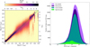 |
Fig. 9 Statistics of the photometric and spectroscopic redshifts. Left: photo-z posterior distributions as a function of SDSS spectroscopic redshift for LoTSS DR2 sources with reliable spectroscopic redshift (zwarning_sdss = 0) and photo-z estimates that pass the photo-z quality selection (flag_qual = 1). The photo-z distribution is normalized such that the distribution for each zspec bin integrates to unity. Dashed and dotted lines illustrate the bounds zphot = zspec ± 0.05 and 0.15 × (1 + z) respectively. Right: the distribution of available redshifts for all optically identified objects as a function of WISE band 1 magnitude, where a ‘good redshift’ is defined in the text. |
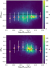 |
Fig. 10 Distribution of estimated stellar mass differences compared to GSWLC (ΔMGSWLC; Salim et al. 2016, 2018, upper panel) and LoTSS Deep Fields DR1 (ΔMDF; Duncan 2022, lower panel) for sources in common. Red circles and corresponding error bars illustrate the median and 16-84th percentile ΔM within a fixed log10(MLoTSS/M⊙) bin. |
9 Catalogue description
The catalogues described in this paper are available online11. Details of the columns are given in Appendix A.
Our main product is a science-ready source catalogue which contains all objects that we think are physical sources, together with their radio properties, their optical ID information, and their associated optical properties if available, our best estimate of redshift combining spectroscopic and photometric constraints, and derived physical quantities as described in the previous section. The source names in this catalogue are the names from the LoTSS DR2 radio source catalogue described by Shimwell et al. (2022), except for composite sources, where the tabulated RA and Dec, and therefore the name, are generated from the flux-weighted mean position of the components that make up the source.
Accompanying the source catalogue is a component catalogue which is essentially an annotated version of the DR2 radio source catalogue, with the following differences:
The name of entries in the catalogue is Component_Name;
Some entries in the original table may have been deleted as artefacts and so will not be present in our component table;
Some components are Gaussians promoted to components as part of the deblending process, and so were not originally present in the DR2 source catalogue: in this case there will be an entry in the Deblended_from column which refers back to the DR2 source catalogue;
All components have a Parent_Source column entry referring to an object in the main source table.
Finally, as noted above, a JSON-format dictionary provides a list of all tags for sources that were tagged by RGZ(L) volunteers. This can easily be iterated over to generate lists of sources with a particular tag, bearing in mind the caveats given in the previous section.
10 Properties of the final catalogue
10.1 Quality comparisons
There are few large fully optically identified radio catalogues in the northern sky with which we can compare our new catalogue. One instructive comparison is with the flux-complete 3CRR catalogue (Laing et al. 1983) which includes full optical identifications and spectroscopic redshifts. Largest angular size (LAS) measurements from high-resolution radio maps are also available12. Because the 3CRR sources are selected to have a flux density >10.9 Jy at 178 MHz (on the scale of Roger et al. 1973) they should all be detected by LoTSS: they are typically large, bright sources and so we would expect (Fig. 8) that many of them will have been associated and identified by visual inspection.
There are 62 3CRR sources in our sky area (Table 6) and all can be identified in the radio catalogue. We crossmatched by first searching for an optical ID matching the 3CRR position within 5 arcsec, and secondly looking for bright (>10 Jy) sources close to the 3CRR catalogued radio position in the LoTSS catalogue. Of the matches, two have no optical ID in the LoTSS catalogue (these are the high-z source 3C 68.2 where an ID might very well not have been detectable given our data, and the quasar 3C 263 where presumably the host was mistaken for a star by some volunteers in RGZ(L)) and three have the wrong ID, all from visual inspection. Given that the optical IDs for the 3CRR sources benefit from high-resolution, high-frequency observations, a correct optical ID fraction of 57/62 (92%) is good; it is noteworthy that all eight IDs derived from the ridge line code are correct. The flux density in LoTSS matches with the extrapolation of the 3CRR flux density to 144 MHz to within 20% in 49/62 (79%) of cases: the sources where there is not a good match tend to be large sources where presumably some components of the radio source were either not detected by ~~PYBDSF~~~ or were not correctly associated. Only a minority of sources (19/62) have LAS measurements in the LoTSS catalogue that match the 3CRR values to within 20%. This is partly because some (11) 3CRR objects are not resolved by LoTSS, but generally the LoTSS sizes, while being correlated with the 3CRR ones, tend to be systematically higher. Reasons for this will include the lower resolution of LoTSS compared to the VLA maps used to measure the 3CRR sizes, which tends to make flood-fill sizes an overestimate, issues with the composite source size discussed in Sect. 7, and possibly in some cases some physical effect where more extended emission is seen at low frequencies.
The LoTSS catalogue includes a redshift accurate to 10% in only 23/62 cases, almost all spectroscopic redshifts from SDSS. The redshift is clearly not expected to be correct in the 5/62 sources that have no or the wrong optical ID, In some cases we have no redshift at all in LoTSS (18/62) – many at high z where Legacy photometry may not be available, but also including low-z sources like 3C 31, 3C 338, and 3C465 where we might have expected to have a SDSS spectroscopic redshift13. 16/62 sources have an inaccurate photometric redshift, failing to match within 10%. The photometric redshifts are only badly wrong in a few cases (the worst is 3C 265 where the true redshift is 0.811 and the photo-z 0.319), and the 3CRR sources contain a large fraction of quasars, as well as galaxies with extremely strong emission lines, where photometric redshifts are likely to be more challenging. Nevertheless this does illustrate the value of a targeted spectroscopic survey of the LoTSS sources, as will be provided by the WEAVE-LOFAR project.
Finally, we confirmed that there are no sources in the LoTSS catalogue that should have been in the 3CRR catalogue but are not, either because of errors in the 3CRR selection or in our association. There are a number of unmatched sources in the overlapping sky area with 144-MHz flux densities > 12 Jy but all are 4C sources with catalogued 178-MHz flux density just below the 3CRR cutoff.
A further useful quality comparison is with the sources in LoTSS DR1 (Williams et al. 2019). Compared to DR2, DR1 benefited from the first stage of visual inspection for association and identification being done by astronomers who were able to inspect a wider range of data (including WISE images and FIRST contours) but relied on poorer LOFAR images with a higher noise level and used shallower PanSTARRS optical data. As noted above, the rate of optical identification is substantially higher in DR2. We matched DR1 and DR2 as closely as possible by restricting a comparison to sky areas where the density of DR1 sources is >500 deg−2, which gave a matching area of 353 deg2. DR1 includes 291 758 sources in this sky area, while DR2 has 401 890: the optical ID fraction is 73.0% in DR1 and 86.8% in DR2, while the fraction of these IDs with redshift estimates is 70.0% in both datasets. Of the 212949 sources in DR1 with IDs, 183 064 (86.0%) have an optical positional crossmatch within 1.5 arcsec with the IDs of DR2 sources, and these are overwhelmingly clearly the same LOFAR source when their DR1 and DR2 total flux density is compared - they show no obvious difference on a scatter plot comparing the total flux densities from sources that are simply crossmatched in radio position (of which there are 267 368, or 91.6% of DR1, within a 3 arcsec match radius). Figure 11 shows that the match fraction is lowest for faint and large sources, and best for bright and compact ones, as expected since we would hope that the LR algorithm would select the same sources in both DR1 and DR2. There is no evidence, comparing Figs. 8 and 11, that any of our optical ID methods from DR2 performs noticeably better or worse relative to DR1 than the others. There is no significant dip in the matching identification fraction at flux levels of a few mJy, suggesting that these sources are not any worse identified in DR2 than in DR1. The non-matching sources are also not uniformly distributed on the sky, which may suggest that per-mosaic astrometric uncertainties or a position-dependent higher fraction of spurious sources in one or other catalogue are responsible for some of the unmatched sources. Overall we view the good agreement between the two independently identified catalogues as positive, but the discrepancies illustrate that we have not yet converged on a process that gives identical optical IDs for a given region of radio and optical sky.
We cross-checked the optical IDs in our catalogue against those derived by O’Sullivan et al. (2023) in their study of 2461 polarized sources in LoTSS DR2 as part of the Magnetism Key Science Project (MKSP): their IDs were derived using a separate private Zooniverse project using the same radio data as us, but carried out by astronomers rather than the public, and using both Legacy and WISE data for optical IDs. The polarized sources on which the catalogue is based are bright and often extended relative to DR2 sources as a whole. O’Sullivan et al. (2023) obtained an 88% optical ID rate, similar to ours overall, but only 76% of their sources with optical IDs have the same IDs in our catalogue. The sizes and flux densities of the MKSP sources place them in the regime where we have the lowest optical ID rates (Fig. 8) and so the discrepancy is not surprising: as noted above, professional astronomers seem to give significantly higher optical ID rates than citizen scientists for extended sources, and WISE images are often better than the Legacy survey for high-z host galaxies. This is a further indication that it might be possible to obtain more IDs with more targeted visual inspection, although at considerably increased cost in time.
Finally, we compared with the results for the first data release (DR1) of the original RGZ project (Wong et al., in prep.), which provides a catalogue of 99 624 sources derived from the FIRST survey, of which 56% have a WISE counterpart ID derived from visual inspection by citizen scientists. Taking the overlapping sky area (all in the ‘Spring’ field of LoTSS DR2) and cutting regions where there is a low density of LoTSS DR2 sources to avoid edge effects, we have around 3000 deg2 in common, with our catalogue containing 2 787 742 sources while the RGZ DR1 catalogue contains 40 690. Of the 23 964 sources from the RGZDR1 sample that have WISE positional IDs, 20411 (85.2%) have a match to an optical position ID in the LoTSS DR2 optical catalogue within 3 arcsec – these are overwhelmingly true matches as can be verified from comparing their WISE magnitudes and radio properties. As with the LoTSS DR1 comparison, this gives confidence in our catalogue, since our hybrid process involving LR matching, heuristics and visual inspection is giving results comparable in quality to a pure visual inspection approach. Wong et al. (in prep.) estimate the reliability of the RGZ DR1 catalogue to be ~70–80%, so our agreement here is as good as would be expected, bearing in mind that for some of these sources RGZ and our catalogue may agree on a common but incorrect source ID. It is interesting to note that the raw ID fraction of RGZ is significantly higher than for our Zooniverse results (Sect. 5): we speculate that this is partly due to the RGZ input catalogue being composed of simpler, brighter radio sources derived from FIRST, and partly due to the use of WISE for the optical identification.
Matches of 3CRR objects with sources in the final Catalogue.
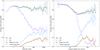 |
Fig. 11 As Fig. 8 but here the fraction of LoTSS DR1 objects that have an optical ID matching the one in DR2 are shown broken down by their origin in DR2. Flux and angular size values here are from DR1. |
10.2 Properties of the sources with optical IDs
Figure 12 (left panel) shows an example of the relation between optical or IR apparent magnitude and 144-MHz flux density for the nearly three million sources with usable photometry in WISE bands 1 and 2. This ‘teapot plot’ (which has a counterpart in the far-IR, e.g. Hardcastle et al. 2016) exhibits two distinct branches, one which shows a clear and close to linear correlation between radio and mid-IR flux for bright galaxies (due to star-forming galaxies on the main sequence of star formation) and one branch with brighter radio sources and fainter IR galaxies, with no clear relationship between radio flux and IR properties, which represents the AGN population (a less clearly defined branch to brighter magnitudes above flux densities of 10 mJy represents the quasar population). These relationships would not appear in a flux-flux plot unless the bulk of our optical identifications were correct. Using the good redshifts available for a subset of the sample, we can see the same relation in physical quantities in the right-hand panel of Fig. 12, where the main sequence of star formation is seen as a diagonal line with a plume of luminous points above it representing the RLAGN population: radio-quiet quasars occupy the right-hand side of the plot. The relatively narrow optical magnitude range occupied by RLAGN is a consequence of the fact that they are much more common in the most massive galaxies (e.g. Sabater et al. 2019). The relation between radio luminosity and absolute magnitude in this plot appears quite tight (with around half a decade of scatter) and persists over ~5 magnitudes. Care would need to be taken in selecting RLAGN using this plot alone, although it is clear that a luminosity cut > 1025 W Hz−1, as used in part by Hardcastle et al. (2019), would efficiently select true radio-excess AGN. We will return to the question of RLAGN selection in this sample in a future paper.
WISE colour-colour plots are widely used to classify optical sources (e.g., Assef et al. 2010; Stern et al. 2012; Gürkan et al. 2014). Figure 13 shows the colour-colour plot for 1.3 million radio-source counterparts with good WISE photometry (by which we mean sources that are detected and have magnitude errors < 0.3 in all three bands). Radio source counterparts are widespread across this plot but normal galaxies occupy a curved locus with a relatively narrow range of W1–W2 colours but considerable spread in W2–W3. Star-forming galaxies, which lie on the main sequence lines in Fig. 12, are concentrated in a relatively small colour space. Away from the normal galaxy locus, we see that the upper part of the plot (with red W1–W2 colours) are mostly high-z objects and therefore largely quasars. Intermediate-z objects lying below the normal galaxy locus with blue W1–W2 colours are non-quasar AGN hosts.
Finally, our mass estimates allow us to look at the relationship between physical quantities such as mass and radio luminosity. Figure 14 shows a plot of the relation between those two for sources with mass estimates flagged as reliable in the catalogue. Again the main sequence of star formation can be seen as a luminosity-mass relation in the lower part of the plot, while RLAGN have radio luminosity independent of mass. A visible horizontal scatter between luminosities of 1024 and 1025 W Hz−1 is the result of contamination by quasars, which do not have accurate mass estimates, as can be seen by considering their WISE colours, but overall this plot shows the expected behaviour and we clearly have the statistics for more detailed studies of the relationship between mass and radio properties in future papers.
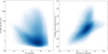 |
Fig. 12 Relations between radio and optical properties of objects in the catalogue. Left: logarithmic density plot of 3 226 797 WISE-detected DR2 sources showing total LOFAR flux density against WISE band 2 AB magnitude. Right: logarithmic density plot of 851 356 DR2 sources with good WISE magnitudes and zbest < 0.5 showing total 144-MHz radio luminosity against WISE band 2 absolute AB magnitude, with approximate K-correction using the W1–W2 colour. |
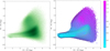 |
Fig. 13 Catalogued objects in the WISE color-colour space. Left: WISE colour-colour logarithmic density plot for 1 273 882 objects with good WISE photometry in the radio catalogue. Right: the same plot but showing the median redshift in each bin for the subset of 1 119 991 objects with good WISE photometry and also well-defined zbest < 4, overlaid with KDE-estimated logarithmic density contours. |
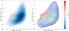 |
Fig. 14 Relationship between mass and radio luminosity for objects in the catalogue. Left: logarithmic density plot of radio luminosity as a function of mass for 1 737 778 radio sources with good mass estimates and usable W1 and W2 magnitudes. Right: the same plot but showing the median W1 – W2 colours for each cell, overlaid with KDE-estimated logarithmic density contours. |
10.3 Extreme sources
Another way of investigating the quality of the catalogue is to sort by measured or inferred physical quantities to search for sources with extreme properties, which could be present in error. The brightest radio sources in the catalogue, as discussed above (Sect. 10.1) are the 3CRR objects, and these are on the whole correctly identified with their host galaxies. The largest sources in terms of angular size include the degree-scale radio galaxy NGC 315, the giant radio galaxies 3C 236 and 3C 31, various other less well-known large FRI sources, and the spiral galaxy M101: none of the largest ten objects in the catalogue appear to be spurious associations, with the least plausible being ILTJ010331.88+230426.1, a putative large FRII source. There are 89 sources in the catalogue with angular sizes >10 arcmin. Because our catalogue is based on the 6-arcsec imaging, the images used for visual inspection had limited sensitivity to extended structure, and so we do not expect to see all the large sources found in visual inspection of lower-resolution images (Oei et al. 2022, 2023).
Turning to physical quantities, the highest-redshift radio source in our catalogue is at z = 6.6: as discussed above, all sources with z > 5 come from the high-redshift quasar catalogue of Gloudemans et al. (2022). For objects with reliable redshifts we can look at radio luminosity estimates. The most luminous object in our catalogue is 3C 196 at z = 0.870 (Table 6), followed by the z = 3.03 object ILTJ142921.88+540611.2 (6C B142744.1+541929), both at around 2 × 1029 W Hz−1. In total there are 25 objects with radio luminosity >1029 W Hz−1. This is the level that is reached by the most powerful 3CRR sources and corresponds to jet powers around 1040 W (Hardcastle et al. 2019). The vast majority of these powerful sources have redshifts that come from the SDSS quasar catalogue and so are as reliable as the SDSS redshifts: most are unresolved in the radio so their optical IDs are not in doubt. It is noteworthy that there are none of these very powerful sources at z ≳ 4, presumably because the nature of AGN accretion or environments and/or the very high radiative losses to inverse-Compton emission prevent them from occurring, since we could certainly detect them if they were optically identified.
Finally we can look at the physically largest sources. Our largest object, ILTJ152932.89+601538.1, has a nominal size of 6.9 Mpc, though we caution that this relies on a photometric redshift of 0.916, a slightly too large estimated angular size, and an uncertain identification. However, even if identified instead with the z = 0.798 galaxy associated with ILTJ152933.05+601552.6 and given a hand-measured size of 827 arcsec, its reduced computed size of 6.2 Mpc would still make it the largest radio galaxy known to date. Including this object, which will be discussed further by Oei et al. (in prep.), and ILTJ110838.03+291731.4, which at 5.7 Mpc becomes the second largest giant candidate discovered, there are 13 candidate sources with projected size >4 Mpc, all of which are convincing FRII radio galaxies on inspection, and four of which have spectroscopic redshifts. However, the optical IDs for these large angular size sources should be treated with caution as there could be multiple candidate hosts for each source. In total in the catalogue there are 8541 sources with estimated physical size >700 kpc, the standard threshold for a ‘giant’ radio source (Machalski et al. 2006) in a modern cosmology, though careful size measurements will be necessary to confirm whether they meet this threshold value.
10.4 Caveats and user advice
There are a number of potential issues affecting the scientific use of a catalogues of optical IDs like this one. Here we outline a few points that users of the catalogue should be aware of.
The first and most obvious issue is that the catalogue is not complete, in the technical sense that we do not have optical IDs for all the radio sources in the catalogue; moreover, we do not have redshifts for all the sources that have optical IDs. This limitation comes primarily from the optical and IR data available: the optical ID catalogues for the LoTSS deep fields (Kondapally et al. 2021) demonstrate that it is possible to get much closer to completeness, even for a radio survey significantly deeper than DR2, if one has substantially deeper optical and IR data than we have over the whole northern sky. When using the wide-area catalogue, though, the incompleteness means that one cannot, for example, select on radio properties such as radio luminosity and be certain that one has selected all the sources that physically should have been selected. Given that only 57% of sources have a good spectroscopic or photometric redshift, the bias introduced by incompleteness could be substantial, though it is likely to affect predominantly low-mass and/or high-redshift objects. So, for example, it is reasonable to expect that the catalogue is close to complete for low-z massive galaxies, but the catalogue user needs to conduct their own tests to quantify and account for the effects of this incompleteness for their science use case. For example, standard completeness correction techniques for the construction of luminosity functions for populations need to take account of the non-trivial selection functions for both optical ID and redshift incompleteness.
A more subtle issue is that the catalogue only lists objects that are detected in the original DR2 radio catalogue (Shimwell et al. 2022). Flux densities measured for detected objects should be reasonably secure, though it is important to consider the effects of detection incompleteness, Eddington bias and the possibility that a source might not be fully deconvolved at the faint end. Most of these issues can be avoided by applying a higher flux density cut to the catalogue, such as the 1.1 mJy flux density reported by Shimwell et al. (2022) to be the 95% completeness limit. The flux density scale for DR2 is accurate to the 5-10% level (Hardcastle et al. 2021). However, if a catalogue user wishes to measure the LoTSS maximum-likelihood flux density for a known pre-existing sample of optical objects, they should proceed in two stages. First they should cross-match their sample on optical position with the present catalogue, which will almost always give the best estimate of the radio properties of a given optical galaxy that appears here, including the effects of extended or multi-component sources. Secondly, they should return to the LoTSS images to estimate the flux measurements (or, if desired and appropriate to the analysis being conducted, upper limits) for objects that do not appear in this catalogue, which takes account both of the non-uniform noise in the LoTSS images and of sources that may be genuinely detected but are missing from the LoTSS radio catalogue. Neglecting the second step and considering only objects found in the present catalogue is likely to lead to a significantly biased analysis.
11 Summary and conclusions
We have found optical IDs and associations for 4.1 million radio sources in the LoTSS DR2 area. At more than an order of magnitude larger than our previous work in DR1 (Williams et al. 2019), this is by far the largest optically identified radio survey yet carried out. In addition to the extensive use of likelihood-ratio (LR) cross-matching, including the ridge-line analysis of Barkus et al. (2022), we made use of ~950 000 visual inspections by citizen scientist volunteers and ~150 000 by astronomers, including filtering, too-zoomed-in, and blend workflows as well as the internal Zooniverse project. We roughly estimate the human time cost of these inspections, based on a notional 30 s per object and a standard working pattern, at around six person-years.
We achieve an 85.0% optical ID rate, and the science-ready catalogue that we generate includes high-quality photometric redshifts for the optical IDs, spectroscopic redshifts from SDSS and HETDEX where possible, and, for the 58% of sources with a good redshift estimate, derived quantities including radio luminosity and physical size estimates. Galaxy mass estimates are also provided as a by-product of the photometric redshift process. A comparison with the bright, extended sources in the 3CRR catalogue (Laing et al. 1983) shows that the quality of our optical identifications and redshift estimates is generally good for this class of object. Followup with WEAVE-LOFAR (Smith et al. 2016) will obtain spectroscopic redshifts for most of the ~330 000 bright sources in the sample with flux density >8 mJy, which may include many high-z radio galaxies. This is the first work to combine (at scale) statistical, citizen science, and expert matching based on homogeneous radio source extraction parameters and multi-wavelength ancillary data, paving the way toward incorporating more advanced matching techniques that will prove crucial to work using SKA and LSST surveys.
The use of a citizen science project for work such as this, while immensely rewarding to the participants and the science team alike, is time-consuming and, as discussed in Sect. 5, gives relatively low optical identification rates which have to be supplemented by expert visual inspection and/or additional algorithms. For the still larger task of generating optical IDs for the remainder of the full LoTSS northern sky survey, and for future surveys with the SKA, it will be essential to learn from the results of this work. While human visual inspection seems hard to avoid for the most complex sources, algorithms for association (Mostert et al. 2022) and optical identification (Barkus et al. 2022) may soon be able to deal with a much larger fraction of radio sources. The associations and identifications that we have generated may be used to train future generations of machine-learning algorithms.
Our publicly released catalogue should provide a resource for a vast number of scientific projects based on the radio properties of active and star-forming galaxies. We expect to make future releases of the catalogues incorporating improved optical IDs, further spectroscopic redshifts including those from HETDEX, WEAVE, and DESI, and environmental and radio spectral information.
Although LoTSS is currently largely generating images using only the Dutch baselines of LOFAR, with a typical resolution of 6 arcsec, a stretch goal of the project is to exploit the much higher resolution provided by the full International LOFAR Telescope (ILT), which can be ~0.3 arcsec at 144 MHz (Morabito et al. 2022), over large areas of the sky. Exploitation of all-sky highresolution imaging, when available, should significantly improve the optical identification rate.
In addition to this problem, wide-area high-resolution surveys with the VLA, such as FIRST, are also necessarily strongly surface-brightness limited because of the small VLA field of view, which means that short observations are required in order to cover wide areas. In the case of some low-surface brightness structures, such as moderately resolved star-forming galaxies, it is this surface brightness limit thatprevents FIRST from seeing all of their emission rather than missing short baselines; here a VLA survey with a larger beam, such as NVSS, can perform much better (Condon et al. 2002).
A small number of sources, just over 4000 in total, were classified through a test version of the same interface by members of the collaboration before the launch of the public project. These classifications are merged in with the citizen science classifications in the final analysis.
In order of the volume of use by volunteers these were English, French, German, Italian, Polish, Dutch, Swedish, and Chinese.
Where σNMAD = 1.48 × median(|δz| /(1 + zspec)) and the outlier fraction, OLF0.15, is the fraction of sources with |δz| /(1 + zspec) > 0.15, for δz = zphot – zspec.
6978 sources that failed the rms criterion could not be sent to RGZ(L) as they could not be visualized using contour maps. Some of these were deleted as artefacts in subsequent processing, and a few were included in RGZ(L) or post-processing outputs, but many simply end up with a likelihood-ratio ID. In the final catalogue these objects can be selected by requiring Total_flux > 8 mJy, DC_Maj > 15 arcsec and Peak_flux < 2×Isl_rms. They should be treated with caution in the final catalogue.
Model grids are generated separately for the Legacy Surveys North and South datasets separately to account for the differing optical filters, with LoTSS sources fit to the corresponding grid.
From the LOFAR surveys website https://lofar- surveys.org/dr2_release.html or at the CDS.
We use the compilation of data at https://3crr.extragalactic.info/
3C 31 and 3C 465’s hosts are simply missing from the SDSS main galaxy sample, presumably due to the existence of close companions which prevented a fibre being placed on the galaxies (Strauss et al. 2002). 3C 338’s host position in the catalogue is 2.2 arcsec away from the corresponding SDSS catalogue position and therefore it is not picked up by our 1.5-arcsec crossmatch.
Acknowledgements
The full acknowledgments are available in Appendix B.
Appendix A Table descriptions
Table A.1 gives a description of the columns in the source catalogue and Table A.2 gives a description of the columns in the component catalogue.
Columns for the main catalogue. ‘Type’ gives the Python data type and its length in bits.
Appendix B Acknowledgements
We thank an anonymous referee for comments that allowed us to improve the paper. M.J.H., D.J.B.S., and J.C.S.P. acknowledge support from the UK STFC [ST/V000624/1]. M.A.H. acknowledges support from STFC grant [ST/X002543/1]. K.J.D. acknowledges funding from the European Union’s Horizon 2020 research and innovation programme under the Marie Sklodowska-Curie grant agreement no. 892117 (HIZRAD) and support from the STFC through an Ernest Rutherford Fellowship (grant number ST/W003120/1). L.A. is grateful for support from the STFC via CDT studentship grant ST/P006809/1. B.B. is grateful for support from the STFC [ST/S505614/1]. J.H.C. acknowledges support from the STFC [ST/T000295/1 and ST/X001164/1]. E.O. acknowledges support from the VIDI research programme with project number 639.042.729, which is financed by the Netherlands Organisation for Scientific Research (NWO). PNB and RK are grateful for support from STFC via grant ST/V000594/1. A.D. acknowledges support by the BMBF Verbundforschung under the grant 05A20STA. CLH acknowledges support from the Lever-hulme Trust through an Early Career Research Fellowship. M.J. acknowledges support from the National Science Centre, Poland under grant UMO-2018/29/B/ST9/01793. M.K.B. acknowledges support from the National Science Centre, Poland under grant no. 2017/26/E/ST9/00216. M.H. thanks the Ministry of Education and Science of the Republic of Poland for support and granting funds for the Polish contribution to the International LOFAR Telescope (arrangement no. 2021/WK/02) and for maintenance of the LOFAR PL-612 Baldy station (MSHE decision no. 28/530020/SPUB/SP/2022). F.dG. acknowledges the support of the ERC CoG grant number 101086378. S.P.O. acknowledges support from the Comunidad de Madrid Atraccion de Talento program via grant 2022-T1/TIC-23797. I.P. acknowledges support from INAF under the Large Grant 2022 funding scheme (project “MeerKAT and LOFAR Team up: a Unique Radio Window on Galaxy/AGN co-Evolution)”. D.J.S. acknowledges support by the project “NRW-Cluster for data intensive radio astronomy: Big Bang to Big Data (B3D)” funded through the programme “Profilbildung 2020”, an initiative of the Ministry of Culture and Science of the State of North Rhine-Westphalia. HT gratefully acknowledges the support from the Shuimu Tsinghua Scholar Program of Tsinghua University, the fellowship of China Postdoctoral Science Foundation 2022M721875, and long lasting support from JBCA machine learning group and Doa Tsinghua machine learning group. M.V. acknowledges financial support from the Inter-University Institute for Data Intensive Astronomy (IDIA), a partnership of the University of Cape Town, the University of Pretoria, the University of the Western Cape and the South African Radio Astronomy Observatory, and from the South African Department of Science and Innovation’s National Research Foundation under the ISARP RADIOSKY2020 Joint Research Scheme (DSI-NRF Grant Number 113121) and the CSUR HIPPO Project (DSI-NRF Grant Number 121291).
LOFAR is the Low Frequency Array, designed and constructed by ASTRON. It has observing, data processing, and data storage facilities in several countries, which are owned by various parties (each with their own funding sources), and which are collectively operated by the ILT foundation under a joint scientific policy. The ILT resources have benefited from the following recent major funding sources: CNRS-INSU, Observatoire de Paris and Université d’Orléans, France; BMBF, MIWF-NRW, MPG, Germany; Science Foundation Ireland (SFI), Department of Business, Enterprise and Innovation (DBEI), Ireland; NWO, The Netherlands; The Science and Technology Facilities Council, UK; Ministry of Science and Higher Education, Poland; The Istituto Nazionale di Astrofisica (INAF), Italy.
This research made use of the Dutch national e-infrastructure with support of the SURF Cooperative (e-infra 180169) and the LOFAR e-infra group. The Jülich LOFAR Long Term Archive and the German LOFAR network are both coordinated and operated by the Jülich Supercomputing Centre (JSC), and computing resources on the supercomputer JUWELS at JSC were provided by the Gauss Centre for Supercomputing e.V. (grant CHTB00) through the John von Neumann Institute for Computing (NIC).
This research made use of the University of Hertfordshire high-performance computing facility and the LOFAR-UK computing facility located at the University of Hertfordshire (https://uhhpc.herts.ac.uk) and supported by STFC [ST/P000096/1], and of the Italian LOFAR IT computing infrastructure supported and operated by INAF, and by the Physics Department of Turin University (under an agreement with Con-sorzio Interuniversitario per la Fisica Spaziale) at the C3S Supercomputing Centre, Italy.
This research made use of ASTROPY, a community-developed core Python package for astronomy (Astropy Collaboration 2013) hosted at http://www.astropy.org/, of MATPLOTLIB (Hunter 2007), of APLPY, an open-source astronomical plotting package for Python hosted at https://aplpy.github.io/, and of TOPCAT and STILTS (Taylor 2005).
The Legacy Surveys consist of three individual and complementary projects: the Dark Energy Camera Legacy Survey (DECaLS; Proposal ID #2014B-0404; PIs: David Schlegel and Arjun Dey), the Beijing-Arizona Sky Survey (BASS; NOAO Prop. ID #2015A-0801; PIs: Zhou Xu and Xiaohui Fan), and the Mayall z-band Legacy Survey (MzLS; Prop. ID #2016A-0453; PI: Arjun Dey). DECaLS, BASS and MzLS together include data obtained, respectively, at the Blanco telescope, Cerro Tololo Inter-American Observatory, NSF’s NOIRLab; the Bok telescope, Steward Observatory, University of Arizona; and the Mayall telescope, Kitt Peak National Observatory, NOIR-Lab. The Legacy Surveys project is honoured to be permitted to conduct astronomical research on Iolkam Du’ag (Kitt Peak), a mountain with particular significance to the Tohono O’odham Nation.
NOIRLab is operated by the Association of Universities for Research in Astronomy (AURA) under a cooperative agreement with the National Science Foundation.
This project used data obtained with the Dark Energy Camera (DECam), which was constructed by the Dark Energy Survey (DES) collaboration. Funding for the DES Projects has been provided by the U.S. Department of Energy, the U.S. National Science Foundation, the Ministry of Science and Education of Spain, the Science and Technology Facilities Council of the United Kingdom, the Higher Education Funding Council for England, the National Center for Supercomputing Applications at the University of Illinois at Urbana-Champaign, the Kavli Institute of Cosmological Physics at the University of Chicago, Center for Cosmology and Astro-Particle Physics at the Ohio State University, the Mitchell Institute for Fundamental Physics and Astronomy at Texas A&M University, Financiadora de Estudos e Projetos, Fundacao Carlos Chagas Filho de Amparo, Financiadora de Estudos e Projetos, Fundacao Carlos Chagas Filho de Amparo a Pesquisa do Estado do Rio de Janeiro, Conselho Nacional de Desenvolvimento Cientifico e Tecno-logico and the Ministerio da Ciencia, Tecnologia e Inovacao, the Deutsche Forschungsgemeinschaft and the Collaborating Institutions in the Dark Energy Survey. The Collaborating Institutions are Argonne National Laboratory, the University of California at Santa Cruz, the University of Cambridge, Centro de Investiga-ciones Energeticas, Medioambientales y Tecnologicas-Madrid, the University of Chicago, University College London, the DES-Brazil Consortium, the University of Edinburgh, the Eidgenössische Technische Hochschule (ETH) Zurich, Fermi National Accelerator Laboratory, the University of Illinois at Urbana-Champaign, the Institut de Ciencies de l’Espai (IEEC/CSIC), the Institut de Fisica d’Altes Energies, Lawrence Berkeley National Laboratory, the Ludwig Maximilians Universität Munchen and the associated Excellence Cluster Universe, the University of Michigan, NSF’s NOIRLab, the University of Nottingham, the Ohio State University, the University of Pennsylvania, the University of Portsmouth, SLAC National Accelerator Laboratory, Stanford University, the University of Sussex, and Texas A&M University.
BASS is a key project of the Telescope Access Program (TAP), which has been funded by the National Astronomical Observatories of China, the Chinese Academy of Sciences (the Strategic Priority Research Program “The Emergence of Cos-mological Structures” Grant # XDB09000000), and the Special Fund for Astronomy from the Ministry of Finance. The BASS is also supported by the External Cooperation Program of Chinese Academy of Sciences (Grant # 114A11KYSB20160057), and Chinese National Natural Science Foundation (Grant # 11433005).
This project, and the Legacy Survey project, makes use of data products from the Near-Earth Object Wide-field Infrared Survey Explorer (NEOWISE), which is a project of the Jet Propulsion Laboratory/California Institute of Technology. NEOWISE is funded by the National Aeronautics and Space Administration.
The Legacy Surveys imaging of the DESI footprint is supported by the Director, Office of Science, Office of High Energy Physics of the U.S. Department of Energy under Contract No. DE-AC02-05CH1123, by the National Energy Research Scientific Computing Center, a DOE Office of Science User Facility under the same contract; and by the U.S. National Science Foundation, Division of Astronomical Sciences under Contract No. AST-0950945 to NOAO.
HETDEX is led by the University of Texas at Austin McDonald Observatory and Department of Astronomy with participation from the Ludwig-Maximilians-Universität München, Max-Planck-Institut für Extraterrestrische Physik (MPE), Leibniz-Institut für Astrophysik Potsdam (AIP), Texas A&M University, Pennsylvania State University, Institut für Astrophysik Göttingen, The University of Oxford, Max-Planck-Institut für Astrophysik (MPA), The University of Tokyo and Missouri University of Science and Technology.
Observations for HETDEX were obtained with the Hobby-Eberly Telescope (HET), which is a joint project of the University of Texas at Austin, the Pennsylvania State University, Ludwig-Maximilians-Universität München, and GeorgAugust-Universität Göttingen. The HET is named in honor of its principal benefactors, William P. Hobby and Robert E. Eberly. The Visible Integral-field Replicable Unit Spectrograph (VIRUS) was used for HETDEX observations. VIRUS is a joint project of the University of Texas at Austin, Leibniz-Institut für Astrophysik Potsdam (AIP), Texas A&M University, MaxPlanck-Institut für Extraterrestrische Physik (MPE), Ludwig-Maximilians-Universität München, Pennsylvania State University, Institut für Astrophysik Göttingen, University of Oxford, and the Max-Planck-Institut für Astrophysik (MPA).
Funding for HETDEX has been provided by the partner institutions, the National Science Foundation, the State of Texas, the US Air Force, and by generous support from private individuals and foundations.
This research used data obtained with the Dark Energy Spectroscopic Instrument (DESI). DESI construction and operations is managed by the Lawrence Berkeley National Laboratory. This material is based upon work supported by the U.S. Department of Energy, Office of Science, Office of High-Energy Physics, under Contract No. DE-AC02-05CH11231, and by the National Energy Research Scientific Computing Center, a DOE Office of Science User Facility under the same contract. Additional support for DESI was provided by the U.S. National Science Foundation (NSF), Division of Astronomical Sciences under Contract No. AST-0950945 to the NSF’s National Optical-Infrared Astronomy Research Laboratory; the Science and Technologies Facilities Council of the United Kingdom; the Gordon and Betty Moore Foundation; the Heising-Simons Foundation; the French Alternative Energies and Atomic Energy Commission (CEA); the National Council of Science and Technology of Mexico (CONACYT); the Ministry of Science and Innovation of Spain (MICINN), and by the DESI Member Institutions: https://www.desi.lbl.gov/collaborating-institutions. The DESI collaboration is honored to be permitted to conduct scientific research on Iolkam Du’ag (Kitt Peak), a mountain with particular significance to the Tohono O’odham Nation. Any opinions, findings, and conclusions or recommendations expressed in this material are those of the author(s) and do not necessarily reflect the views of the U.S. National Science Foundation, the U.S. Department of Energy, or any of the listed funding agencies.
References
- Ahumada, R., Prieto, C. A., Almeida, A., et al. 2020, ApJS, 249, 3 [Google Scholar]
- Alegre, L., Sabater, J., Best, P., et al. 2022, MNRAS, 516, 4716 [NASA ADS] [CrossRef] [Google Scholar]
- Almosallam, I. A., Jarvis, M. J., & Roberts, S. J. 2016a, MNRAS, 462, 726 [NASA ADS] [CrossRef] [Google Scholar]
- Almosallam, I. A., Lindsay, S. N., Jarvis, M. J., & Roberts, S. J. 2016b, MNRAS, 455, 2387 [NASA ADS] [CrossRef] [Google Scholar]
- Assef, R. J., Kochanek, C. S., Brodwin, M., et al. 2010, ApJ, 713, 970 [NASA ADS] [CrossRef] [Google Scholar]
- Assef, R. J., Stern, D., Kochanek, C. S., et al. 2013, ApJ, 772, 26 [Google Scholar]
- Astropy Collaboration (Robitaille, T. P., et al.) 2013, A & A, 558, A33 [NASA ADS] [CrossRef] [EDP Sciences] [Google Scholar]
- Banfield, J. K., Wong, O. I., Willett, K. W., et al. 2015, MNRAS, 453, 2326 [Google Scholar]
- Barkus, B., Croston, J. H., Piotrowska, J., et al. 2022, MNRAS, 509, 1 [Google Scholar]
- Becker, R. H., White, R. L., & Helfand, D. J. 1995, ApJ, 450, 559 [Google Scholar]
- Bennett, A. S. 1962, MmRAS, 68, 163 [NASA ADS] [Google Scholar]
- Best, P. N., & Heckman, T. M. 2012, MNRAS, 421, 1569 [NASA ADS] [CrossRef] [Google Scholar]
- Blanton, M. R., Bershady, M. A., Abolfathi, B., et al. 2017, AJ, 154, 28 [Google Scholar]
- Boyce, M. M., Hopkins, A. M., Riggi, S., et al. 2023, PASA, 40, e027 [NASA ADS] [CrossRef] [Google Scholar]
- Bruzual, G., & Charlot, S. 2003, MNRAS, 344, 1000 [NASA ADS] [CrossRef] [Google Scholar]
- Chabrier, G. 2003, PASP, 115, 763 [Google Scholar]
- Chambers, K. C., Magnier, E. A., Metcalfe, N., et al. 2016, ArXiv e-prints [arXiv:1612.85568] [Google Scholar]
- Charlot, S., & Fall, S. M. 2000, ApJ, 539, 718 [Google Scholar]
- Chen, H., & Garrett, M. A. 2021, MNRAS, 507, 3761 [NASA ADS] [CrossRef] [Google Scholar]
- Condon, J. J., Cotton, W. D., Greisen, E. W., et al. 1998, AJ, 115, 1693 [Google Scholar]
- Condon, J. J., Cotton, W. D., & Broderick, J. J. 2002, AJ, 124, 675 [Google Scholar]
- Croston, J. H., Hardcastle, M. J., Mingo, B., et al. 2019, A & A, 622, A10 [NASA ADS] [CrossRef] [EDP Sciences] [Google Scholar]
- Dabhade, P., Röttgering, H. J. A., Bagchi, J., et al. 2020, A & A, 635, A5 [NASA ADS] [CrossRef] [EDP Sciences] [Google Scholar]
- de Gasperin, F., Williams, W. L., Best, P., et al. 2021, A & A, 648, A104 [CrossRef] [EDP Sciences] [Google Scholar]
- DESI Collaboration (Adame, A. G., et al.) 2023, AJ, submitted [arXiv:2386.86388] [Google Scholar]
- Dey, A., Schlegel, D. J., Lang, D., et al. 2019, AJ, 157, 168 [Google Scholar]
- Duncan, K. J. 2022, MNRAS, 512, 3662 [NASA ADS] [CrossRef] [Google Scholar]
- Duncan, K. J., Conselice, C. J., Mortlock, A., et al. 2014, MNRAS, 444, 2960 [Google Scholar]
- Duncan, K. J., Conselice, C. J., Mundy, C., et al. 2019, ApJ, 876, 110 [Google Scholar]
- Duncan, K. J., Kondapally, R., Brown, M. J. I., et al. 2021, A & A, 648, A4 [NASA ADS] [CrossRef] [EDP Sciences] [Google Scholar]
- Euclid Collaboration (Scaramella, R., et al.) 2022, A & A, 662, A112 [NASA ADS] [CrossRef] [EDP Sciences] [Google Scholar]
- Gebhardt, K., Mentuch Cooper, E., Ciardullo, R., et al. 2021, ApJ, 923, 217 [NASA ADS] [CrossRef] [Google Scholar]
- Gendre, M. A., & Wall, J. V. 2008, MNRAS, 390, 819 [NASA ADS] [Google Scholar]
- Gloudemans, A. J., Duncan, K. J., Saxena, A., et al. 2022, A & A, 668, A27 [NASA ADS] [CrossRef] [EDP Sciences] [Google Scholar]
- Gower, J. F. R., Scott, P. F., & Wills, D. 1967, MmRAS, 71, 49 [NASA ADS] [Google Scholar]
- Gürkan, G., Hardcastle, M. J., & Jarvis, M. J. 2014, MNRAS, 438, 1149 [CrossRef] [Google Scholar]
- Gürkan, G., Hardcastle, M. J., Best, P. N., et al. 2019, A & A, 622, A11 [CrossRef] [EDP Sciences] [Google Scholar]
- Hardcastle, M. J., Gürkan, G., van Weeren, R. J., et al. 2016, MNRAS, 462, 1910 [Google Scholar]
- Hardcastle, M. J., Williams, W. L., Best, P. N., et al. 2019, A & A, 622, A12 [NASA ADS] [CrossRef] [EDP Sciences] [Google Scholar]
- Hardcastle, M. J., Shimwell, T. W., Tasse, C., et al. 2021, A & A, 648, A10 [CrossRef] [EDP Sciences] [Google Scholar]
- Hunter, J. D. 2007, Comput. Sci. Eng., 9, 90 [NASA ADS] [CrossRef] [Google Scholar]
- Jin, S., Trager, S. C., Dalton, G. B., et al. 2023, MNRAS, in press, https://doi.org/18.1893/mnras/stad557 [Google Scholar]
- Kondapally, R., Best, P. N., Hardcastle, M. J., et al. 2021, A & A, 648, A3 [CrossRef] [EDP Sciences] [Google Scholar]
- Lacy, M., Baum, S. A., Chandler, C. J., et al. 2020, PASP, 132, 035001 [Google Scholar]
- Laing, R. A., Riley, J. M., & Longair, M. S. 1983, MNRAS, 204, 151 [NASA ADS] [CrossRef] [Google Scholar]
- Levi, M., Bebek, C., Beers, T., et al. 2013, ArXiv e-prints [arXiv: 1388.8847] [Google Scholar]
- Lotka, A. J. 1926, J. Washington Acad. Sci., 16, 317 [Google Scholar]
- Lyke, B. W., Higley, A. N., McLane, J. N., et al. 2020, ApJS, 250, 8 [NASA ADS] [CrossRef] [Google Scholar]
- Machalski, J., Jamrozy, M., Zola, S., & Koziel, D. 2006, A & A, 454, 85 [NASA ADS] [CrossRef] [EDP Sciences] [Google Scholar]
- Mainzer, A., Bauer, J., Grav, T., et al. 2011, ApJ, 731, 53 [Google Scholar]
- Mentuch Cooper, E., Gebhardt, K., Davis, D., et al. 2023, ApJ, 943, 177 [NASA ADS] [CrossRef] [Google Scholar]
- Mingo, B., Croston, J. H., Hardcastle, M. J., et al. 2019, MNRAS, 488, 2701 [NASA ADS] [CrossRef] [Google Scholar]
- Mohan, N., & Rafferty, D. 2015, Astrophysics Source Code Library [record ascl:1582.887] [Google Scholar]
- Morabito, L. K., Matthews, J. H., Best, P. N., et al. 2019, A & A, 622, A15 [NASA ADS] [CrossRef] [EDP Sciences] [Google Scholar]
- Morabito, L. K., Jackson, N. J., Mooney, S., et al. 2022, A & A, 658, A1 [NASA ADS] [CrossRef] [EDP Sciences] [Google Scholar]
- Mostert, R. I. J., Duncan, K. J., Alegre, L., et al. 2022, A & A, 668, A28 [NASA ADS] [CrossRef] [EDP Sciences] [Google Scholar]
- Oei, M. S. S. L., van Weeren, R. J., Hardcastle, M. J., et al. 2022, A & A, 660, A2 [NASA ADS] [CrossRef] [EDP Sciences] [Google Scholar]
- Oei, M. S. S. L., van Weeren, R. J., Gast, A. R. D. J. G. I. B., et al. 2023, A & A, 672, A163 [CrossRef] [EDP Sciences] [Google Scholar]
- O’Sullivan, S. P., Shimwell, T. W., Hardcastle, M. J., et al. 2023, MNRAS, 519, 5723 [CrossRef] [Google Scholar]
- Pacifici, C., Iyer, K. G., Mobasher, B., et al. 2023, ApJ, 944, 141 [NASA ADS] [CrossRef] [Google Scholar]
- Rankine, A. L., Matthews, J. H., Hewett, P. C., et al. 2021, MNRAS, 502, 4154 [CrossRef] [Google Scholar]
- Rawlings, S., Lacy, M., Leahy, J. P., et al. 1996, MNRAS, 279, L13 [NASA ADS] [CrossRef] [Google Scholar]
- Roger, R. S., Costain, C. H., & Bridle, A. H. 1973, AJ, 78, 1030 [Google Scholar]
- Rudnick, L. 2021, Galaxies, 9, 85 [NASA ADS] [CrossRef] [Google Scholar]
- Sabater, J., Best, P. N., Hardcastle, M. J., et al. 2019, A & A, 622, A17 [NASA ADS] [CrossRef] [EDP Sciences] [Google Scholar]
- Sabater, J., Best, P. N., Tasse, C., et al. 2021, A & A, 648, A2 [CrossRef] [EDP Sciences] [Google Scholar]
- Salim, S., Lee, J. C., Janowiecki, S., et al. 2016, ApJS, 227, 2 [NASA ADS] [CrossRef] [Google Scholar]
- Salim, S., Boquien, M., & Lee, J. C. 2018, ApJ, 859, 11 [Google Scholar]
- Schlafly, E. F., Meisner, A. M., & Green, G. M. 2019, ApJS, 240, 30 [Google Scholar]
- Shimwell, T. W., Röttgering, H. J. A., Best, P. N., et al. 2017, A & A, 598, A104 [NASA ADS] [CrossRef] [EDP Sciences] [Google Scholar]
- Shimwell, T. W., Hardcastle, M. J., Tasse, C., et al. 2022, A & A, 659, A1 [CrossRef] [EDP Sciences] [Google Scholar]
- Smith, D. J. B., Best, P. N., Duncan, K. J., et al. 2016, in SF2A-2016: Proceedings of the Annual meeting of the French Society of Astronomy and Astrophysics, eds. C. Reylé, J. Richard, L. Cambrésy, et al., 271 [Google Scholar]
- Stern, D., Assef, R. J., Benford, D. J., et al. 2012, ApJ, 753, 30 [Google Scholar]
- Strauss, M. A., Weinberg, D. H., Lupton, R. H., et al. 2002, AJ, 124, 1810 [Google Scholar]
- Sutherland, W., & Saunders, W. 1992, MNRAS, 259, 413 [Google Scholar]
- Tasse, C., Shimwell, T., Hardcastle, M. J., et al. 2021, A & A, 648, A1 [NASA ADS] [CrossRef] [EDP Sciences] [Google Scholar]
- Taylor, M. B. 2005, ASP Conf. Ser., 347, 29 [Google Scholar]
- van Haarlem, M. P., Wise, M. W., Gunst, A. W., et al. 2013, A & A, 556, A2 [CrossRef] [EDP Sciences] [Google Scholar]
- Wang, L., Gao, F., Duncan, K. J., et al. 2019, A & A, 631, A109 [NASA ADS] [CrossRef] [EDP Sciences] [Google Scholar]
- Williams, W. L., Hardcastle, M. J., Best, P. N., et al. 2019, A & A, 622, A2 [NASA ADS] [CrossRef] [EDP Sciences] [Google Scholar]
- Wright, E. L., Eisenhardt, P. R. M., Mainzer, A. K., et al. 2010, AJ, 140, 1868 [Google Scholar]
- Zheng, X. C., Röttgering, H. J. A., Best, P. N., et al. 2020, A & A, 644, A12 [NASA ADS] [CrossRef] [EDP Sciences] [Google Scholar]
All Tables
Columns for the main catalogue. ‘Type’ gives the Python data type and its length in bits.
All Figures
|
Fig. 1 Sky coverage of the LoTSS DR2 (blue) and the Legacy DR9 (yellow and orange) optical surveys. The purple lines (‘MW’) show the Galactic plane and lines of |b| = 10°. As described in the text, ‘Legacy North’ data is made up of BASS and MzLS data, ‘Legacy South’ data are from DECaLS. |
| In the text | |
|
Fig. 2 Representation of the decision tree used to process all entries in the PYBDSF catalogue lying in the Legacy Survey sky area. Following this workflow a decision is made for each source whether to: (i) make the optical and IR identification, or lack thereof, through the LR method (blue and red outcomes respectively); (ii) process the source in RGZ(L) (green outcomes, including direct RGZ(L) post-processing); (iii) reject the source as an artefact (grey outcomes). The key parameters are defined in Table 1. The number and percentage of PYBDSF sources in each final bin are shown for each final outcome. Some faint sources are not processed further (orange outcomes); these are discussed in the text. |
| In the text | |
|
Fig. 3 Example of the three images presented to citizen scientists for one catalogued LOFAR radio source (ILTJ093236.46+602825.5). Left panel, the default view: radio contours from the LOFAR data (logarithmically increasing by a factor two at each interval from five times the local noise level) are superposed on the Legacy three-colour image. Cyan ellipses denote catalogued radio sources, with sizing as described in the text; the solid ellipse is the one under study and dotted ellipses represent other sources in the radio catalogue. Middle panel: the colour scale shows the LOFAR radio data only. Right panel: a view of the optical sky only. This image is 2 arcmin on a side. |
| In the text | |
|
Fig. 4 Images from the classification section of the Zooniverse interface. This shows the three task screens presented for one catalogued source, ILTJ172125.82+370417.2, seen by the user in the order top left, top right, bottom left panels. The image shown here is 100 arcsec on a side. All three views here show the standard image (Legacy colour scale, radio contours, and ellipses to represent catalogued Gaussians). In the first panel, the marker for an associated component can be seen; in the second panel, the user has also marked an optical identification for the radio source. In the third panel, the user has the opportunity to apply various flags to the source or to discuss it on the talk pages. Note the unassociated radio source to the southeast (bottom left). The toolbar below the image allows the user to switch images, to get information on the source, to invert the colour map, or to add the source to a list of favourites. Additionally, the user has the option to zoom, pan, and rotate the image using the buttons on the right. |
| In the text | |
|
Fig. 5 Statistics of the Zooniverse volunteer population. Left: histogram showing the numbers of Zooniverse volunteers who made a certain number of classifications. On a log scale the rough power-law distribution of classification numbers is apparent, with a slope ≈ − 1. Right: histogram of the distribution of optical ID consensus scores for volunteers with more than 100 classifications. |
| In the text | |
|
Fig. 6 Examples of RGZ(L) subjects with the optical and radio contour image seen by Zooniverse platform volunteers overplotted with the optical IDs selected by the volunteers, marked as green crosses. All sources have five or more optical ID selections (volunteers could optionally select more than one possible ID). The top row shows examples where a consensus was achieved and the correct optical ID selected, the bottom row ones where no consensus was found and no optical ID returned from RGZ(L). |
| In the text | |
|
Fig. 7 Example user interface for the ‘Second deblend’ workflow. In an interactive Matplotlib window the expert classifier has separated the emission from two extended sources that had been combined in PYBDSF, seen in green and cyan, and has selected optical IDs for both. An unrelated source marked in white has been left unchanged. The new source is a mixture of PYBDSF components (solid lines) and Gaussians (dashed lines). |
| In the text | |
|
Fig. 8 Fractional optical IDs in the DR2 catalogue. The two plots show the total fraction of optically identified objects, and the breakdown by different methods of optical identification, as a function of (left) total flux density of the resulting source and (right) catalogued largest angular size. |
| In the text | |
|
Fig. 9 Statistics of the photometric and spectroscopic redshifts. Left: photo-z posterior distributions as a function of SDSS spectroscopic redshift for LoTSS DR2 sources with reliable spectroscopic redshift (zwarning_sdss = 0) and photo-z estimates that pass the photo-z quality selection (flag_qual = 1). The photo-z distribution is normalized such that the distribution for each zspec bin integrates to unity. Dashed and dotted lines illustrate the bounds zphot = zspec ± 0.05 and 0.15 × (1 + z) respectively. Right: the distribution of available redshifts for all optically identified objects as a function of WISE band 1 magnitude, where a ‘good redshift’ is defined in the text. |
| In the text | |
|
Fig. 10 Distribution of estimated stellar mass differences compared to GSWLC (ΔMGSWLC; Salim et al. 2016, 2018, upper panel) and LoTSS Deep Fields DR1 (ΔMDF; Duncan 2022, lower panel) for sources in common. Red circles and corresponding error bars illustrate the median and 16-84th percentile ΔM within a fixed log10(MLoTSS/M⊙) bin. |
| In the text | |
|
Fig. 11 As Fig. 8 but here the fraction of LoTSS DR1 objects that have an optical ID matching the one in DR2 are shown broken down by their origin in DR2. Flux and angular size values here are from DR1. |
| In the text | |
|
Fig. 12 Relations between radio and optical properties of objects in the catalogue. Left: logarithmic density plot of 3 226 797 WISE-detected DR2 sources showing total LOFAR flux density against WISE band 2 AB magnitude. Right: logarithmic density plot of 851 356 DR2 sources with good WISE magnitudes and zbest < 0.5 showing total 144-MHz radio luminosity against WISE band 2 absolute AB magnitude, with approximate K-correction using the W1–W2 colour. |
| In the text | |
|
Fig. 13 Catalogued objects in the WISE color-colour space. Left: WISE colour-colour logarithmic density plot for 1 273 882 objects with good WISE photometry in the radio catalogue. Right: the same plot but showing the median redshift in each bin for the subset of 1 119 991 objects with good WISE photometry and also well-defined zbest < 4, overlaid with KDE-estimated logarithmic density contours. |
| In the text | |
|
Fig. 14 Relationship between mass and radio luminosity for objects in the catalogue. Left: logarithmic density plot of radio luminosity as a function of mass for 1 737 778 radio sources with good mass estimates and usable W1 and W2 magnitudes. Right: the same plot but showing the median W1 – W2 colours for each cell, overlaid with KDE-estimated logarithmic density contours. |
| In the text | |
Current usage metrics show cumulative count of Article Views (full-text article views including HTML views, PDF and ePub downloads, according to the available data) and Abstracts Views on Vision4Press platform.
Data correspond to usage on the plateform after 2015. The current usage metrics is available 48-96 hours after online publication and is updated daily on week days.
Initial download of the metrics may take a while.