| Issue |
A&A
Volume 678, October 2023
|
|
|---|---|---|
| Article Number | A58 | |
| Number of page(s) | 12 | |
| Section | Stellar structure and evolution | |
| DOI | https://doi.org/10.1051/0004-6361/202346932 | |
| Published online | 05 October 2023 | |
Peering into the tilted heart of Cyg X-1 with high-precision optical polarimetry
1
Department of Physics and Astronomy, 20014 University of Turku, Finland
e-mail: vakrau@utu.fi
2
Nordita, KTH Royal Institute of Technology and Stockholm University, Hannes Alfvéns väg 12, 10691 Stockholm, Sweden
3
Nicolaus Copernicus Astronomical Center, Polish Academy of Sciences, Bartycka 18, 00-716 Warszawa, Poland
4
Department of Physics and Astronomy, East Tennessee State University, Johnson City, TN 37614, USA
5
Graduate School of Sciences, Tohoku University, Aoba-ku, 980-8578 Sendai, Japan
6
Leibniz-Institut für Sonnenphysik, Schöneckstr. 6, 79104 Freiburg, Germany
7
Istituto Ricerche Solari Aldo e Cele Daccò (IRSOL), Faculty of Informatics, Università della Svizzera italiana, 6605 Locarno, Switzerland
Received:
18
May
2023
Accepted:
3
August
2023
We present high-precision optical polarimetric observations of the black hole X-ray binary Cygnus X-1 that span several cycles of its 5.6-day orbital period. The week-long observations on two telescopes located in opposite hemispheres allowed us to track the evolution of the polarization within one orbital cycle with the highest temporal resolution to date. Using the field stars, we determined the interstellar polarization in the source direction and subsequently its intrinsic polarization Pint = 0.82%±0.15% with a polarization angle θint = 155° ±5°. The optical polarization angle is aligned with that in the X-rays recently obtained with the Imaging X-ray Polarimetry Explorer. Furthermore, it is consistent within the uncertainties with the position angle of the radio ejections. We show that the intrinsic polarization degree is variable with the orbital period with an amplitude of ∼0.2% and discuss various sites of its production. Assuming that the polarization arises from a single Thomson scattering of the primary star radiation by the matter that follows the black hole in its orbital motion, we constrained the inclination of the binary orbit i > 120° and its eccentricity e < 0.08. The asymmetric shape of the orbital profiles of the Stokes parameters also implies the asymmetry of the scattering matter distribution in the orbital plane, which may arise from the tilted accretion disk. We compared our data to the polarimetric observations made in 1975–1987 and find good agrement within 1° between the intrinsic polarization angles. On the other hand, the polarization degree decreased by 0.4% over half a century, suggesting secular changes in the geometry of the accreting matter.
Key words: accretion / accretion disks / black hole physics / polarization / stars: black holes / stars: individual: Cyg X-1 / X-rays: binaries
© The Authors 2023
 Open Access article, published by EDP Sciences, under the terms of the Creative Commons Attribution License (https://creativecommons.org/licenses/by/4.0), which permits unrestricted use, distribution, and reproduction in any medium, provided the original work is properly cited.
This article is published in open access under the Subscribe to Open model. Subscribe to A&A to support open access publication.
1. Introduction
The determination of the large-scale accretion geometry and orbital parameters of X-ray binaries is a fundametally important problem. Various techniques can be employed to examine the geometry of these systems, such as photometry, spectroscopy, imaging, and timing. A special place in this list belongs to polarimetry, which is known to be most sensitive to changes in geometry. The geometrical properties can be determined by tracking the changes in polarization degree (PD) and polarization angle (PA) as a function of the orbital phase. The stochastic variability on timescales comparable to the orbital period may significantly alter the average polarization profile. Dense coverage of an entire orbital cycle is needed to reliably determine the accretion geometry, shape, and orientation of the binary components.
The orbital parameters in binary systems are conventionally studied using optical and infrared polarimetry. For the low-mass X-ray binaries in outburst, emission in these wavelengths can be composed of several components: an (irradiated) accretion disk, a wind, a jet, and a hot accretion flow (Poutanen & Veledina 2014; Uttley & Casella 2014). Optical polarimetry has been used as a fine tool for distinguishing between them (Veledina et al. 2019; Kosenkov et al. 2020). In (near-)quiescence, optical polarimetry has helped constrain the role of the non-stellar components in total spectra (Kravtsov et al. 2022) and to determine the misalignment of the black hole (BH) and orbital spins (Poutanen et al. 2022). For high-mass X-ray binaries, emission in the infrared, optical, and ultraviolet bands is completely dominated by the donor star. The emission can be scattered by different large-scale components in the binary such as the accretion stream, disk, outflow or jet. The polarization signal in this case can reveal the location, orientation, and physical properties of the scattering component (Jones et al. 1994).
With the launch of the Imaging X-ray Polarimetry Explorer (IXPE; Weisskopf et al. 2022), the polarimetric field gained a second wind. It became possible to directly link the orientation of the large-scale binary components that are probed by the optical and infrared wavelengths to the innermost accretion geometry with the help of X-ray polarimetry. The prototypical BH X-ray binary Cygnus X-1 became the first target of these studies (Krawczynski et al. 2022). The week-long IXPE exposure has been accompanied by the global multiwavelength campaigns, allowing it to cover a large fraction of its 5.6 d orbital period.
Cyg X-1 is the first discovered BH X-ray binary and a well-studied system (Bowyer et al. 1965). It is a persistent source and a high-mass binary hosting a supergiant ∼40 M⊙ donor star of spectral type O in a nearly circular orbit (eccentricity e ∼ 0.02) with the most massive Galactic BH MBH = 21.2 ± 2.1 M⊙ known to date (Miller-Jones et al. 2021). The donor is close to filling its Roche lobe, and the compact object accretes the matter through the focused stellar wind (Gies & Bolton 1986a). Accretion proceeds through the disk, whose emission is often seen in the X-rays (Gierliński et al. 1997, 1999; Zdziarski & Gierliński 2004), and a fraction of matter leaves the system in the form of the jet (Stirling et al. 2001; Fender et al. 2006; Miller-Jones et al. 2021).
Optical radiation is dominated by the light of the companion star and shows pronounced variations at an orbital period that is caused by the asymmetric shape of the donor (Kemp et al. 1983; Gies & Bolton 1986b; Brocksopp et al. 1999b; Orosz et al. 2011). Optical polarization measurements also show pronounced orbital variability (Nolt et al. 1975). The observed double-peak sinusoidal variations of the PD and PA are consistent with the scenario in which polarization arises from Thomson scattering of the donor star radiation by optically thin matter located within the binary (Brown et al. 1978; Milgrom 1978). This pattern is typical for binary systems and was observed in a variety of sources from classical (Piirola 1980; Berdyugin & Harries 1999) to gamma-ray binaries (Kravtsov et al. 2020). The synchronization with the orbital phase indicates that the source of the polarization is connected to the orbital motion of the BH around the companion star.
Polarization may originate from the accretion stream, its impact point on the accretion disk or the disk matter itself, or it might be related to the outflow/jet. Which component causes variations in the polarization in Cyg X-1 is unknown. The shapes of the PD and PA profiles have been used in several works to constrain orbital parameters such as inclination and eccentricity (Kemp et al. 1978, 1983; Karitskaya 1981; Dolan & Tapia 1989; Nagae et al. 2009).
The long orbital period of Cyg X-1 became an obstacle to tracking the polarimetric variations over a large fraction of a single cycle, and the average profile was obtained by including data from many cycles. This approach may lead to a substantial deviation of the obtained mean profile from the individual cycles, however, because the system is known to show substantial superorbital variability (Priedhorsky et al. 1983; Karitskaya et al. 2001; Poutanen et al. 2008; Zdziarski et al. 2011). This means that the scattering matter gradually rearranges within the binary over the superorbital period, leading to a systematic bias in the determination of the binary inclination from the mean orbital profile. On the other hand, the data obtained during a single orbital period at one telescope are unavoidably under-sampled (Dolan & Tapia 1989; Nagae et al. 2009). We performed multi-observatory polarimetric observations of Cyg X-1 that for the first time covered up to 30% of the orbit in one cycle. This was achieved by observing with nearly identical polarimeters from telescopes that were separated by ∼140° in longitude.
In this paper, we present the results of joint analysis of the new high-precision optical polarimetric observations of Cyg X-1, historical polarimetric data obtained in 1975–1987, and optical flux measurements, which allowed us to make a new attempt to qualitatively and quantitatively constrain the geometry of Cyg X-1. The paper is organized as follows. In Sect. 2 we describe the observations of the source and of the field stars to determine the contribution of the interstellar polarization. In Sect. 3 we present the main results of the study: the variations in the polarization on different timescales. We present a model for the observed orbital and superorbital variability of the polarization in Sect. 4. Finally, we summarize our findings in Sect. 5.
2. Data acquisition and analysis
We performed high-precision optical polarimetric observations of Cyg X-1 with the broad-band BVR polarimeters DIPol-2 (Piirola et al. 2014) and DIPol-UF (Piirola et al. 2021). DIPol-2 is mounted on the remotely controlled 60 cm Tohoku telescope (T60) at Haleakala Observatory, Hawaii. DIPol-UF is a visitor instrument installed at the 2.56 m Nordic Optical Telescope (NOT) at the Observatorio del Roque de los Muchachos (ORM) on La Palma, Spain. DIPol-2 and DIPol-UF are high-precision double-image CCD polarimeters, capable of measuring polarization simultaneously in three optical (BVR) bands. The polarization of the sky (even if it changes during observations) is optically eliminated by the design of the instruments. The instrumental polarization of both instruments is low (< 10−4) and is well calibrated by observing 15–20 unpolarized standard stars. The zero-point of the PA was determined by observing the highly polarized standards HD 204827 and HD 161056. Each measurement of the Stokes parameters (qobs, uobs) took about 20 s, and more than 200 individual measurements were obtained during the average observing night. A more detailed description of the methods and calibrations can be found in Piirola et al. (2020) and Kravtsov et al. (2022).
Cyg X-1 was observed for 27 nights between 2022 March 28 and July 28 at the T60 and for 6 nights, 2022 May 15–21, at the NOT (see Table 1). Taking advantage of the ∼140° difference in the longitude of the observatories, we covered 30% of the orbit of Cyg X-1 simultaneously with IXPE observations (red stripe in Fig. 1). We refer to this dataset as season 2 (or just S2) hereafter. The typical errors on the 30-min-averaged measurement of the Stokes parameters are σp ≈ 0.004% for the NOT and ≈0.01% for the T60 data.
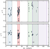 |
Fig. 1. Observed normalized Stokes parameters for Cyg X-1 in the B band. The vertical dotted black lines limit the observational seasons S1 and S3. The two vertical dashed red lines show the start and end of the IXPE campaign on 2022 May 15–21 (season 2). The vertical solid purple lines show the start and end of the TESS observations. |
Log of the polarimetric observations of Cyg X-1.
We additionally used the historical observations carried out at the Pine Mountain Observatory (PMO), United States, in 1975–1987 (see Table 1 and Fig. 2). The reduced data were presented in parts in several papers (Kemp et al. 1978, 1979, 1983), but have never been published as a raw dataset. With the kind permission of the Pine Mountain Observatory staff, we are publishing these data (hereafter PMO data) in the public domain for the first time1.
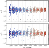 |
Fig. 2. Long-term variations in the normalized Stokes parameters q and u of Cyg X-1, measured in 1975–1987. The vertical dashed lines separate 11 observing seasons, which is roughly equal to one year of observations. The red crosses show season-averaged values. |
The description of the observational techniques can be found in Kemp & Barbour (1981). Each PMO observation is a nightly average value with a typical integration time of several hours. We also used previously unpublished polarimetric observations of Cyg X-1, carried out in 2002 April–May with the TurPol polarimeter (Piirola 1973, 1988), installed on NOT, and with the 60 cm KVA telescope, ORM, La Palma.
In addition to the polarimetric data, we retrieved and analyzed the publicly available2 Transiting Exoplanet Survey Satellite (TESS; Ricker et al. 2014) optical light curves of Cyg X-1. We used calibrated data with a 2-min cadence (PDCSAP_FLUX), obtained in sectors 54 and 55 (2022 July – September; see Fig. 3).
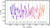 |
Fig. 3. TESS optical light curve of Cyg X-1. The vertical dashed lines separate the consecutive orbital periods T1–T11. |
3. Results
3.1. Average intrinsic polarization and its secular changes
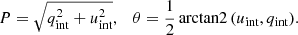
The observed polarization of Cyg X-1 is the sum of the intrinsic polarization of the source and the interstellar (IS) polarization component that arises from the dichroism of the dust grains located between the observer and the target. The IS polarization was estimated and subtracted from the observed polarization. To find a reliable estimate of IS polarization in the source direction, we observed a sample of six field stars (see Fig. 4) that are close to Cyg X-1, as indicated by their Gaia parallaxes (see Fig. 5). We considered the wavelength dependence of the observed polarization (to exclude stars with intrinsic polarization) and took both the angular separation and proximity to the target into account. We conclude that the polarization of star Ref 2 from our sample can serve as the IS polarization estimate. Hereafter, we denote the normalized Stokes parameters of Ref 2 as (qIS, uIS) and subtract them from the observed values of the target (qobs, uobs) to obtain the Stokes parameters of the intrinsic polarization (qint, uint). These are translated into the intrinsic PD P and angle θ,
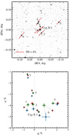 |
Fig. 4. Finding chart and polarization properties of Cyg X-1 and the field stars. Top panel: polarization map for Cyg X-1 and the field stars. The length of the bars corresponds to the PD, and the direction corresponds to the PA (measured from north to east). Bottom panel: observed normalized Stokes parameters q and u for Cyg X-1 (stars) and field stars (circles). The blue, green, and red points with 1σ error bars correspond to the B, V, and R filters, respectively. |
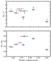 |
Fig. 5. Dependence of the PD (top panel) and PA (bottom panel) on the Gaia parallax for Cyg X-1 (red circle) and the field stars (black circles) in the R band. The horizontal error bars correspond to the errors on the Gaia parallaxes. The errors on the PD and PA are smaller than the symbol size. |
The uncertainty on the PD is equal to the uncertainty of the individual Stokes parameters, and uncertainty on the PA in radians was estimated as σθ = σp/(2P) (Serkowski 1962; Kosenkov et al. 2017). The average observed and intrinsic polarization of Cyg X-1, as well as the interstellar polarization estimates, are listed in Table 2.
Observed PD and PA, interstellar polarization, and intrinsic polarization of Cyg X-1, obtained by averaging S1–S3 data.
A large fraction of the observed polarization, about 4% out of a total 4.5–5%, has an IS origin (Kemp et al. 1979; Nagae et al. 2009). Subtracting the interstellar component from the observed polarization, we find an intrinsic PD of 0.8%±0.2% with a PA of 155° ±5° (or equivalently, −25°; see Table 2). This value is comparable to the characteristic optical PDs in other accreting BH X-ray binaries in outburst (Kosenkov et al. 2017; Veledina et al. 2019). The average intrinsic optical PA matches that measured in the X-rays within the errors (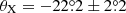 , Krawczynski et al. 2022).
The uniquely long history of polarimetric studies of Cyg X-1 allowed us to track the long-term evolution of the average PD almost 50 years back. We split the PMO V-band observations into 11 bins (PMO1–PMO11; see Fig. 2), each about a year long, and calculated the average values of the observed Stokes parameters within each bin. We plot them in the (q, u) diagram in Fig. 6 (colored crosses) along with our NOT+T60 2022 average polarization (red circle), KVA+NOT 2002 data (empty circle), and other published data (orange square and green diamond; Dolan & Tapia 1989; Nagae et al. 2009). We show the estimated value of the IS polarization with a blue square.
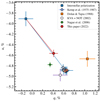 |
Fig. 6. Normalized Stokes parameters (qobs, uobs) of Cyg X-1 in the V band. The red circle with the error bar is the average polarization of Cyg X-1 in 2022. The crosses of different colors (from cool to warm) with error bars correspond to the average polarization in each of the 11 seasons of PMO observations in 1975–1987. The dashed blue and solid red lines show the directions of the average intrinsic polarization vector of Cyg X-1 for PMO and our observations, respectively. The other symbols correspond to the data obtained in other epochs, as described in the inset. |
The blue and red lines connect the PMO and NOT+T60 2022 data with the IS estimate, respectively. The length and direction (from the IS estimate toward the data points) of these lines correspond to the vectors of the average intrinsic polarization for different epochs. The vector directions match with a high accuracy (Δθint < 1°). This supports our choice of the reference star Ref 2 as an estimate of interstellar polarization because the alignment of the intrinsic polarization vectors is unlikely to be accidental. We note that the other historical values shown in Fig. 6 are substantially scattered in the q − u plane, despite their small error bars. This may be caused by the orbital variations: At least several different orbital periods must be averaged to obtain a robust estimate of the average polarization.
The average intrinsic polarization for our NOT+T60 2022 data differs significantly from the PMO data (|ΔPint|≈0.4%), indicating secular changes in the PD while preserving a constant PA. The decrease in the intrinsic PD may be caused by the decrease in the scattered flux, tailored to the secular changes of the wind density, changes in the accretion disk size, and/or its spatial orientation. Figure 2 shows that the one-year polarization averages change slightly from one season to the next. The different spread of all data points shows that the amplitude of the variability also varies on yearly timescales.
3.2. Short-term variability of the orbital profiles
The significant variability in the Stokes (qobs, uobs) parameters with an amplitude of about 0.1%–0.2% is clearly visible in our 2022 observations (see Fig. 1). We performed a timing analysis of our BVR polarimetric data that revealed that the main variation period of the Stokes parameters has not changed since the 1970s and is equal to half of the orbital period within the errors. To study the possible changes in the average orbital profiles of the polarization over decades, we folded our data and the PMO polarization data with the orbital phase, adopting the period Porb from the photometric ephemeris (Brocksopp et al. 1999a). To suppress the stochastic and instrumental noise, we split the data into 18 orbital phase bins, in which we calculated weighted average values of the Stokes parameters that were subsequently used to obtain the PD P and PA θ. The comparison of our light curve and the PMO polarization light curves is shown in Fig. 7. Except for the systematic offset between our and PMO data, the nature of which is discussed above, the shapes of the average PD and PA orbital profiles agree exceptionally well with each other.
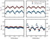 |
Fig. 7. Orbital profiles of the observed and intrinsic polarization of Cyg X-1. Left panels: observed PD, P, (top panel) and PA, θ, (bottom panel) of Cyg X-1 in the V band, folded with the orbital period. The blue circles correspond to the data obtained in 2022. The red crosses correspond to the PMO data obtained in 1975–1987. Each point corresponds to the average value, calculated within a phase bin of width Δϕ = 1/18. The typical 1σ uncertainty is smaller than the symbol size. Right panels: same as the left panel, but showing the intrinsic polarization of Cyg X-1. |
To determine how the shape of optical light curves changes from one period to another, we split TESS photometric data into 11 consecutive orbital periods T1–T11 (see Fig. 3). The shape of each individual profile is far from the double-sine wave that is expected in the case of ellipsoidal variations that are caused by the rotation of a tidally distorted star around the center of mass. A short-period variability is superimposed on the main double-sine curve, which leads to changes in the amplitudes and phases of the main maxima/minima. In Fig. 8 we show the orbital profiles of the intrinsic polarization in R band together with TESS photometric profiles. The optical polarization and optical flux both show double-sinusoidal orbital variations with minima in the conjunctions (phases 0 and 0.5) and maxima in the quadratures (phases 0.25 and 0.75).
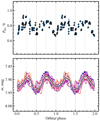 |
Fig. 8. Orbital profiles of the polarization and flux of Cyg X-1 in the optical band. Top panel: intrinsic polarization of Cyg X-1 in the R filter, folded with the orbital period (seasons 1–3 are plotted). Each circle with the 1σ error bar shows the average polarization, calculated within a 30-min bin. Bottom panel: TESS magnitude of Cyg X-1, folded with the orbital period. Different colors (from cold to warm) correspond to different orbital periods T1–T11. The solid black line shows the average orbital profile. |
Photometric variations arise from the nonspherical shape of the tidally distorted companion, whose visible area (and hence the flux) is largest around the quadratures. If the scattering of the donor star emission occurs in a region that is connected to the compact object, we expect the scattering angle to reach a maximum of 90° in the same phases, corresponding to the maximum PD in the case of Thomson scattering. In the conjunctions, the visible area of the supergiant approaches its minima, resulting in the lowest flux, while at the same time, the scattering angle reaches minimum or maximum, leading to a smaller PD. The short-term changes in both the flux and polarization, which are superimposed on the periodic variations, can originate from one or more mechanisms: the pulsations of the main star, spots on its surface, inhomogeneities of the wind, or eclipses of the bright parts of the disk by the infalling matter. We note that despite the correlation of flux and polarization, the polarization variability cannot be explained by variations in the unpolarized flux alone. For the intrinsic PD P = Fpol/Ftot ∼ 0.01, the unpolarized flux variations of about ΔFtot ∼ 5 × 10⁻³Ftot give a negligibly small polarization variability:
while the observed one is at least factor 20 of larger.
With our exceptionally dense orbital coverage, we can compare the profiles of a single cycle with the average one, as given by the PMO data. In Fig. 9 we show the profile obtained from the 8-day-long monitoring of Cyg X-1 during season 2, overlaid on the average profile of the polarization variability in the V band. The figure shows that although the overall shapes of the polarization variability curves are roughly consistent with the patterns of 1975–1987, the amplitude of the variations is substantially higher in our season 2 data, where the harmonic content is also richer. These facts support the statement of Dolan & Tapia (1989) about the existence of nonorbital polarization variability and the importance to account for it when extracting orbital parameters. In the following sections, we describe the modeling of the polarization variability curves with different analytical models and discuss how the short-term variability affects the results.
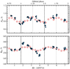 |
Fig. 9. Variability in the intrinsic PD (upper panel) and PA (bottom panel) of Cyg X-1 in V band, measured in May 2022 (blue circles). Each circle corresponds to the average value, calculated within a 30-min bin. The 1σ errors are smaller than the symbol size. The red crosses correspond to the average binned polarization, measured by Kemp with colleagues during 1975–1987, with a constant shift in PD by ΔP = −0.4%. |
3.3. Superorbital evolution of polarization profiles
In addition to the short-term variability, indications of long-term changes in the Cyg X-1 polarization profiles have been reported by several authors. Kemp et al. (1983) suggested long-term optical polarization variations at the superorbital period of 294 d, discovered in the X-rays (Priedhorsky et al. 1983). The authors discussed several models that could explain the variations, including the precession of the accretion disk and the obscuration of the scattering medium. Comparing the average optical polarization obtained between 1975 and 2006, Nagae et al. (2009) found secular variations in the average polarization component of Cyg X-1.
We find signatures of the long-term variability in our 2022 polarimetric data. Figure 10 shows the change in the polarization profiles with superorbital phase, separated roughly by a month (see Fig. 1). The changes in the average values of Stokes parameters along with the changes in the amplitude and profiles of the orbital variations are significant. In Fig. 11 we show the superorbital profile of the V-band polarization of Cyg X-1. The average values of the PD for seasons S1 – S3 (empty red circles), folded with the superorbital period (Psup = 294 d, JD0 = 2 440 000), are consistent with the same part of the superorbital profile as observed in PMO data.
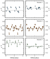 |
Fig. 10. Orbital variations in the observed normalized Stokes parameters q (left) and u (right) of Cyg X-1 in the B band for different seasons (seasons 1, 2, and 3 from top to bottom). The horizontal dashed lines show the weighted average values of the corresponding parameters. |
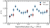 |
Fig. 11. Intrinsic PD of Cyg X-1 in the V band for PMO (blue circles) and S1–S3 (empty red circles) data, folded with the superorbital period. The red points are shifted by a constant ΔP = −0.4% in the vertical direction to take secular changes in the PD into account. |
4. Modeling
To explain the behavior of the polarization at different timescales, we considered several possibilities for the geometry of scattering matter. We started with the generic model for polarization production in binary systems, in which polarization arises from the Thomson scattering of the companion star radiation by a cloud of an optically thin matter near the compact object (Brown et al. 1978). The key assumption of the model is the corotation of the scattering material with the secondary, in our case, with the compact object. The PD in this case peaks at orbital phases at which the scattering angle is 90°. For a circular orbit, the Stokes parameters of the linear polarization vary as a sine-like wave at twice the orbital frequency. In the case of eccentric orbit and/or asymmetry of the distribution of the light-scattering material about the orbital plane, the profiles become skewed and can be described by adding the first harmonic of the orbital period. Alternatively, the appearance of the first harmonic can be related to the presence of an optically thick scattering material. Below, we study the harmonic content of the polarization profiles and consider different possibilities for the geometry of the scattering matter.
4.1. Fourier method
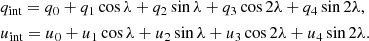
The polarization profiles corresponding to the case of the optically thin corotating scatterer in a circular orbit can be decomposed into Fourier series of the orbital longitude λ = 2πϕ (where ϕ is the orbital phase),
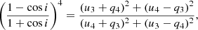
We employed Bayesian inference implemented as the Markov chain Monte Carlo (MCMC; Goodman & Weare 2010) ensemble sampler in the emcee package (Foreman-Mackey et al. 2013) in PYTHON to fit the orbital profiles of the Stokes parameters observed during season S2 with Eq. (2). The best-fit curves are shown in Fig. 12. Following the approach described in Drissen et al. (1986) and Kravtsov et al. (2020), we used the obtained Fourier coefficients to derive the inclination i of the binary,
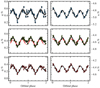 |
Fig. 12. Variability in the observed Stokes parameters of Cyg X-1, obtained during season 2 in B, V, and R bands (top, middle, and bottom panels, respectively). Each circle corresponds to the average value, calculated within a 30-min bin. The 1σ errors are smaller than the symbol size. The solid black lines correspond to the best fit with the Fourier series given by Eq. (2). The dashed red lines in the middle panels show the best fit of PMO historical V -band data with the same model, shifted vertically to overlap our data. |
and the position angle Ω of the orbital axis on the sky,
where
By fitting the orbital polarization profiles obtained in S2 with Eq. (2), we obtained formal values of the inclination i = 125° ±5° (i > 90° indicates the clockwise apparent motion of the compact object on the sky) and the position angle Ω = 129° ±5° of the orbital axis on the sky. However, the formal errors on the estimated orbital parameters obtained from the error propagation are underestimated and hence do not correspond to their actual confidence intervals, which are determined primarily by the internal properties of the model (2) and the amplitude of the stochastic variability in the data. The inclination estimates corresponding to the best-fit Fourier coefficients are always biased toward higher values (Aspin et al. 1981; Simmons et al. 1982; Wolinski & Dolan 1994). The confidence intervals on the orbital parameters for different signal-to-noise ratios can be obtained using Fig. 4 of Wolinski & Dolan (1994): 1σ and 2σ confidence intervals were calculated for four levels of data quality given by γ = 0.5N(A/σp)2, where σp is the standard deviation of noise in the data, A is the amplitude of the polarimetric variability, and N is the number of observations. Our value of γobs = 0.5 × 100 × (6.7)2 ≈ 2200 lies between their grid points (γ = 120 000 and γ = 300). To calculate the confidence intervals on the inclination that we obtained for our S2 data, we therefore performed our own Monte Carlo simulations following the procedure described in Wolinski & Dolan (1994): We modeled the Stokes parameters for different values of i ranging from 90° to 180° using the standard Brown et al. (1978) model (Eq. (6) in that paper). Then, we simulated the Gaussian noise in q and u by adding the fluctuations of the variance  . The Fourier model (Eq. (2)) was then fit to the simulated data using the MCMC approach, and the inclination i′ was calculated using Eq. (3). In Fig. 13 we show the inclination estimates i′ (black points) with the 1σ and 2σ confidence intervals (solid blue and red lines) as a function of the true input inclination i.
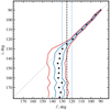 |
Fig. 13. Estimated 1σ and 2σ confidence intervals on the true inclination i for given estimate i′ (solid blue and red lines). The vertical dashed black line corresponds to the best-fit inclination of Cyg X-1. The vertical dotted blue lines correspond to the 1σ error on the best-fit inclination. |
The inclination i ≈ 125° that we derived from the best-fit Fourier coefficients of Cyg X-1 in V and R bands (shown as the dashed vertical black line in Fig. 13) is close to the so-called critical angle  . Above this angle, the 1σ confidence interval on the orbital inclination extends to i = 180° (Wolinski & Dolan 1994). This means that using high-precision polarimetry, we can only place a lower limit of 180° > i > 120° on the inclination value of the Cyg X-1 orbit. We note that previous polarimetrically derived inclination values (Kemp et al. 1978; Dolan & Tapia 1989; Nagae et al. 2009) are most likely overestimated because they were obtained by modeling the data with larger error bars, for which the critical angle is expected to be smaller than
  ∼ 130°. Our lower limit on the inclination i > 120° and the clockwise direction of the orbital motion on the sky are consistent with the value i = 153° ±1° from Miller-Jones et al. (2021).
In contrast to the inclination, the value Ω obtained from Eq. (4) is an unbiased estimate of the true position angle of the projection of the orbital axis on the sky. We used the same MCMC approach as for the inclination to calculate the confidence interval on this angle. Our value Ω = 129° ±10° (or Ω = 129° −180° = − 51° ±10° because of the ±180° ambiguity) is consistent within 3σ with those that were determined by the direction of the intrinsic polarization θint ≈ −25° and the position angle of the jet on the sky Ωjet ≈ −26° (Miller-Jones et al. 2021).
We emphasize that this low accuracy is not a result of the polarization measurement errors (which are smaller than 0.01% for the whole set of our data). Figure 12 shows a remarkable intrinsic scatter of the S2 data points around the fit curves that is especially noticeable for the Stokes q parameter. This aperiodic noise is explained by an additional suborbital variability component that appears on timescales shorter than one orbital cycle. Thus, the key assumption on corotation of the light-scattering material over (at least) a few consecutive orbital cycles does not hold for the Cyg X-1 binary system. Therefore, the traditional Fourier fit up to second harmonics made on polarization data cannot provide meaningful estimates of the orbital inclination, regardless of data quality, quantity, and sampling frequency.
4.2. Eccentric model
While for a circular orbit, theory predicts a smooth change in polarization with the dominant second harmonic of the orbital period, the eccentricity of the orbit shifts all the changes in the polarization toward the periastron. The polarization depends on the scattering angle, which changes according to the orbital motion of the scattering cloud. In the case of an eccentric orbit, this angle changes with different rates in different parts of the orbit, resulting in unequal distances between consecutive maxima/minima of the orbital Stokes parameters curves (this effect was observed for the binary with e ≈ 0.4 in Berdyugin & Tarasov 1998). Therefore, the orbital curves of Stokes parameters can be used for an independent estimation of the orbital eccentricity. We adopted the Thomson scattering model from the appendix of Kravtsov et al. (2020) to describe the orbital changes in the polarization of Cyg X-1. By fitting this model to the V-band season 2 data, we were able to place 3σ upper limit on the eccentricity of Cyg X-1 orbit. The eccecntricity is e < 0.08.
Figure 14 shows the (q, u) plane of the average Stokes parameters of Cyg X-1 obtained during season 2, together with the best-fits with the Fourier series (Eq. (2)) and the model of the Thomson scattering by a cloud on an eccentric orbit (Kravtsov et al. 2020). The latter model (which is a special case of the general BME model for symmetrically distributed matter in the orbital plane) cannot reproduce the pretzel-like shape of the trace left by orbital variations of Cyg X-1 on the (q, u)-plane: The additional source of asymmetry is needed. To explain a similar pattern, Kemp et al. (1978) proposed a model in which the scattering region is eclipsed by the secondary body for half the orbit. This model requires a high (90° > i > 130°) orbital inclination, which contradicts the latest results (including this article).
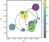 |
Fig. 14. Average Stokes parameters of Cyg X-1 obtained during season 2 in the R band. The color coding and size of the circle correspond to the orbital phase and 1σ uncertainty, respectively. The solid blue curve corresponds to the best fit with the Fourier series given by Eq. (2). The dashed orange line corresponds to the to the best-fit model of a scattering cloud on an eccentric orbit from the appendix of Kravtsov et al. (2020). |
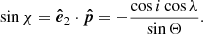
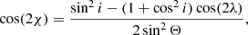
4.3. Polarization by Thomson scattering off a precessing accretion disk
In this section, we present a model of polarization from Thomson scattering by a tilted precessing accretion disk, which can naturally explain the asymmetric pattern of the polarization variability observed in Cyg X-1 without requiring a highly inclined or eccentric orbit. We considered the following geometry: The orbit with an eccentricity e is inclined by an angle i to the line of sight  (Fig. 15). The accretion disk, surrounded by a cloud of electrons, rotates around the optical companion together with the compact object. The disk axis
  is inclined by an angle β to the orbital axis
  (see Fig. 16). The axis of the disk can precess about the orbital axis with the period Tsup.
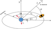 |
Fig. 15. Geometry of the system. Optical emission of the companion star (blue circle at the origin) is scattered by the tilted accretion disk (orange) and the optically thin material (indicated by the black circle in the center of the disk). |
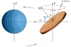 |
Fig. 16. Geometry of the precessing disk. The disk axis |


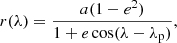
To describe the orbital motion, we introduced the coordinate system ( ,
,  ,
,  ), in which the
  -axis is directed along the orbital axis
  , the vector
  lies in the orbital plane and its projection on the sky is directed to the south, and the vector
  forms the right-handed basis. In this basis,
 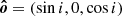 ,
,  , and
, and  . The angle γ is the azimuth of the projection of the disk axis onto the orbital plane measured from
  to
to  . To describe the polarization, we used the polarization basis (
 ,
,  ), in which the vector
 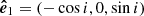 lies along the projection of the vector
  on the plane of the sky, and
 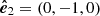 is perpendicular to
  and lies in the plane of the orbit.
The distance between the compact object and the optical companion varies with the orbital longitude λ, measured from  to
to  . It can be expressed as
where a is the semimajor axis of the orbit, and λp is the longitude of the periastron. The unit vector pointing toward the compact object is
and the scattering angle Θ is given by

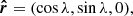
The observed flux Ftot = F* + Fsc is the sum of the flux produced by the optical companion F* and the scattered flux Fsc. We assumed that the latter is produced by Thomson scattering (in an optically thin regime) of stellar radiation by the accretion disk and the surrounding cloud of electrons. In this case, the angular distribution of scattered luminosity can be represented as

where l(μ) = 3(1 + μ2)/8 is the Thomson scattering indicatrix, and  and
and  are fractions of radiation scattered by the cloud and the disk, respectively. In both cases, this fraction is proportional to the total number of free electrons Ne in a cloud/disk and drops with the distance as 1/r2(λ),
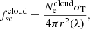
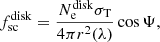
where  . The cos Ψ term is proportional to the effective area of the disk intercepting the stellar radiation, which depends on the position of the disk in the orbit λ and the orientation of its axis
  , defined by two angles: the inclination β of the disk, and its azimuth γ. The latter angle can change with time due to precession as γ = ±2πφsup + γ0, where φsup is the precession phase, and γ0 is the angle γ at zero phase. The sign determines the direction (counterclockwise or clockwise) of the precession.
We scaled  and
and  to the typical values
  and
and  as
as
![$$ \begin{aligned}&f^\mathrm{cloud}_{\rm sc} = f^\mathrm{cloud}_0\ \left[\frac{a(1-e^2)}{r(\lambda )}\right]^2 = f^\mathrm{cloud}_0 \ [1+ e \cos (\lambda -\lambda _{\rm p})]^2,\end{aligned} $$](/articles/aa/full_html/2023/10/aa46932-23/aa46932-23-eq50.gif)
![$$ \begin{aligned}&f^\mathrm{disk}_{\rm sc} = f^\mathrm{disk}_0\ \left[\frac{a(1-e^2)}{r(\lambda )}\right]^2\cos {\Psi }= f^\mathrm{disk}_0 \ [1+ e \cos (\lambda -\lambda _{\rm p})]^2\cos {\Psi }. \end{aligned} $$](/articles/aa/full_html/2023/10/aa46932-23/aa46932-23-eq51.gif)
The PD of scattered radiation in Thomson regime can be expressed in terms of the scattering angle Θ as
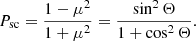
The observer measures the PD P = FscPsc/Ftot of the total flux Ftot, most of which is unpolarized and produced by the optical companion star. The polarized flux of the scattered radiation is
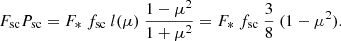
Therefore, the total PD
![$$ \begin{aligned} P = \frac{F_{\rm sc} P_{\rm sc}}{F_{\rm tot}} \approx \frac{3}{8}\ \left[f^\mathrm{cloud}_{\rm sc} + f^\mathrm{disk}_{\rm sc}\right] \ (1-\mu ^2), \end{aligned} $$](/articles/aa/full_html/2023/10/aa46932-23/aa46932-23-eq54.gif)
where we assumed that Fsc ≪ F* and substituted 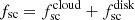 .
.
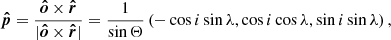
The normalized Stokes parameters of linear polarization are defined as q = Pcos(2χ) and u = Psin(2χ), where χ is the position angle of the polarization pseudo-vector  in the polarization basis (
 ,
,  ),
),
where  . Thus, the expressions for the Stokes parameters can be written as
![$$ \begin{aligned} \begin{aligned}&q = \frac{3}{8} \left[ f^\mathrm{cloud}_{\rm sc} + f^\mathrm{disk}_{\rm sc} \right]\ (1-\mu ^2) \cos (2\chi ), \\&u = \frac{3}{8} \left[ f^\mathrm{cloud}_{\rm sc} + f^\mathrm{disk}_{\rm sc} \right]\ (1-\mu ^2) \sin (2\chi ), \end{aligned} \end{aligned} $$](/articles/aa/full_html/2023/10/aa46932-23/aa46932-23-eq61.gif)
where the polarization angle χ is defined by the expressions
The explicit expressions for cos(2χ) and sin(2χ) are
Combining Eqs. (18) with (21) and (22), we obtain
![$$ \begin{aligned} \begin{aligned}&q = \frac{3}{16} \left[\sin ^2 i - \left(1\!+\!\cos ^2\! i\right) \cos 2\lambda \right]\left[ f^\mathrm{cloud}_{\rm sc} + f^\mathrm{disk}_{\rm sc} \right] , \\&u = -\frac{3}{8} \cos i\ \sin 2\lambda \left[ f^\mathrm{cloud}_{\rm sc} + f^\mathrm{disk}_{\rm sc} \right]. \end{aligned} \end{aligned} $$](/articles/aa/full_html/2023/10/aa46932-23/aa46932-23-eq66.gif)
The  term depends on cos Ψ, reflecting the difference in the amount of scattered radiation for different orientations of the disk axis
  relative to the source of the light. In our model, the disk is not transparent: it has two sides (top and bottom), only one of which is illuminated at any given time. The top of the disk is illuminated when cos Ψ > 0, the bottom of the disk is bright when cos Ψ < 0. The top of the disk is visible for the observer when
  and the bottom of the disk is visible when cos Σ < 0. Therefore, the disk is illuminated and visible only when the product cos Ψ cos Σ is positive, or
  when cos Ψ cos Σ ≤ 0.
To compare the calculations with the observed Stokes parameters (qobs, uobs), the orientation of the orbit on the sky must be taken into account: The projection of the orbital axis on the sky makes an angle Ω with direction to the north (we note that Ω defined in this way differs by π/2 from the longitude of the ascending node that is commonly used instead). The observed Stokes parameters (qobs, uobs) can be obtained by rotating the vector (q, u) by an angle 2Ω,


The modeled Stokes parameters are functions of the orbital longitude λ and need to be computed as functions of the orbital phase ϕ. While for the circular (or nearly circular) orbit, λ can be calculated as λ = 2π(ϕ + ϕp)+λp, where ϕp is the phase of the periastron, for the eccentric orbit, we need to solve Kepler’s equation: From the true anomaly of the orbit λ − λp, we can find the eccentric anomaly E,
and then the mean anomaly M,
which can be converted into the orbital phase as
Thus, the free parameters of the model are the inclination i, the eccentricity e, the longitude of periastron λp, the position angle of the projection of the orbit axis on the sky Ω, the phase of periastron ϕp, the inclination of the disk β and its initial position angle γ0 in the orbital plane, the period of precession Tsup (which can be set to be infinite for the nonprecessing case), and the scattering fractions  and
and  . In order to fit the data, there is a need for additional constant Stokes parameters q0 and u0, which describe the average polarization.
We fit the described model to S2 data by adopting the orbital parameters of Cyg X-1: eccentricity e = 0.02, inclination i = 153° (Miller-Jones et al. 2021), and inclination of the disk β = 20° (Ibragimov et al. 2007). The position angle of the orbital axis was set to be Ω = −26° to match the position angle of the jet. The contributions from the disk and the cloud were assumed to be  and
and  . Because the S2 data cover only one full orbital cycle, the precession period Tsup was set to be much longer than the orbital period so that possible precession of the disk was not taken into account.
The solid blue and dashed red lines in Figs. 17 and 18 show the fits of the model described above to S2 data with and without scattering off the tilted accretion disk, respectively. Although the reduced χ2 of the fits does not differ dramatically (χ2[disk + cloud] = 1.01 versus χ2[cloud] = 1.23), the asymmetric pretzel-like trace of the polarization on the (q, u)-plane cannot be reproduced by the scattering cloud alone. Additionally, the model with the tilted accretion disk predicts the changes in the shape of the orbital polarization profiles with the precession phase: If the superorbital variability observed from the radio to the X-rays is related to the disk precession, the pretzel will make a complete turn around its center once per superorbital period Tsup. To detect this effect, a significant part of the superorbital period must be covered with continuous high-precision optical polarimetric observations.
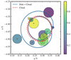 |
Fig. 17. Same as Fig. 14, but showing the model curves at the (q, u)-plane calculated with (solid blue line) and without (dashed red line) scattering by the accretion disk. |
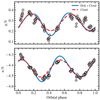 |
Fig. 18. Stokes parameters of Cyg X-1, obtained during season 2 (light crosses) together with the best-fit models with (solid blue line) and without (dashed red line) scattering by the tilted accretion disk. |
5. Summary
We presented new high-precision polarimetric observations of the BH X-ray binary Cyg X-1. Combining them with the 12-year-long PMO observations performed in 1975–1987, we were able to study the polarization behavior at the timescales ranging from hours to decades. The interstellar polarization, which dominates the observed optical polarization Pobs ∼ 4.5%, was accurately measured and subtracted from the data, allowing us to determine the intrinsic polarization of Cyg X-1 as Pint = 0.82%±0.15% with a PA θint = 155° ±5°. The alignment of the X-ray and optical PA, as well as the stability of this angle during the secular PD change, indirectly support our estimate of intrinsic polarization of Cyg X-1. Around-the-clock monitoring of the polarization with two telescopes located in different hemispheres allowed us to track the evolution of the polarization within one orbital cycle with a temporal resolution that is unrivalled so far. The intrinsic polarization of Cyg X-1 shows the orbital variations with two pronounced peaks in the quadratures and two minima in conjugations, most probably produced by Thomson scattering of the companion star radiation by matter that is gravitationally bound to the black hole. The amplitudes of the two consecutive polarization minima measured within one orbital cycle differ significantly, which implies asymmetry of the scattering matter in the orbital plane. We suggest that a tilted accretion disk could be the source of this asymmetry. We find that a misalignment of β ≳ 15° can reproduce the orbital polarization variations. This is in line with the recent finding of a significant misalignment between the orbital and jet axes (Zdziarski et al. 2023). Our modeling of orbital variations in the Stokes parameters allowed us to constrain the eccentricity e < 0.08 and inclination of the orbit i > 120°.
In addition to the orbital variations, we found a significant change (ΔPint ≈ −0.4%) in the average intrinsic PD of Cyg X-1 on a timescales of several decades while preserving the constant intrinsic PA. The decrease in the PD indicates the change in the fraction of scattered radiation, which in turn depends on the amount of scattering material and its effective scattering cross section. This may reflect secular changes in the size/shape of the accretion disk and/or changes in its spatial orientation. We note that the asymmetry of the (q, u)-plane trace of the polarization can be purely artificial. It may result from a complex superposition of periodic and nonperiodic variations and the orbital phase sampling. A long-term high-precision monitoring program with good orbital and superorbital coverage is needed to exclude this.
Analyzing high-precision TESS photometric data, we found stochastic variations of the flux on timescales shorter than the orbital period. Together with the stochastic variability found in the optical polarization, this suggests that one or several additional components are at play: pulsations of the optical companion, spots on its surface, wind clumpiness, eclipses of the bright part of the accretion disk by the infalling matter, and precession of the accretion disk.
Acknowledgments
This paper is based on observations made with the Nordic Optical Telescope, owned in collaboration by the University of Turku and Aarhus University, and operated jointly by Aarhus University, the University of Turku, and the University of Oslo, representing Denmark, Finland, and Norway, the University of Iceland and Stockholm University at the Observatorio del Roque de los Muchachos, La Palma, Spain, of the Instituto de Astrofisica de Canarias. The DIPol-2 and DIPol-UF polarimeters were built in cooperation between the University of Turku, Finland, and the Leibniz-Institut für Sonnenphysik, Germany. We are grateful to the Institute for Astronomy, University of Hawaii, for the allocated observing time. VK acknowledges support from the Vilho, Yrjö and Kalle Väisälä Foundation and Suomen Kulttuurirahasto. AAZ has been supported by the Polish National Science Center under the grant 2019/35/B/ST9/03944.
References
- Aspin, C., Simmons, J. F. L., & Brown, J. C. 1981, MNRAS, 194, 283 [CrossRef] [Google Scholar]
- Berdyugin, A. V., & Harries, T. J. 1999, A&A, 352, 177 [NASA ADS] [Google Scholar]
- Berdyugin, A. V., & Tarasov, A. E. 1998, Astron. Lett., 24, 111 [Google Scholar]
- Bowyer, S., Byram, E. T., Chubb, T. A., & Friedman, H. 1965, Science, 147, 394 [NASA ADS] [CrossRef] [Google Scholar]
- Brocksopp, C., Tarasov, A. E., Lyuty, V. M., & Roche, P. 1999a, A&A, 343, 861 [NASA ADS] [Google Scholar]
- Brocksopp, C., Fender, R. P., Larionov, V., et al. 1999b, MNRAS, 309, 1063 [NASA ADS] [CrossRef] [Google Scholar]
- Brown, J. C., McLean, I. S., & Emslie, A. G. 1978, A&A, 68, 415 [NASA ADS] [Google Scholar]
- Dolan, J. F., & Tapia, S. 1989, PASP, 101, 1135 [NASA ADS] [CrossRef] [Google Scholar]
- Drissen, L., Lamontagne, R., Moffat, A. F. J., Bastien, P., & Seguin, M. 1986, ApJ, 304, 188 [NASA ADS] [CrossRef] [Google Scholar]
- Fender, R. P., Stirling, A. M., Spencer, R. E., et al. 2006, MNRAS, 369, 603 [NASA ADS] [CrossRef] [Google Scholar]
- Foreman-Mackey, D., Hogg, D. W., Lang, D., & Goodman, J. 2013, PASP, 125, 306 [Google Scholar]
- Gierliński, M., Zdziarski, A. A., Done, C., et al. 1997, MNRAS, 288, 958 [CrossRef] [Google Scholar]
- Gierliński, M., Zdziarski, A. A., Poutanen, J., et al. 1999, MNRAS, 309, 496 [CrossRef] [Google Scholar]
- Gies, D. R., & Bolton, C. T. 1986a, ApJ, 304, 389 [NASA ADS] [CrossRef] [Google Scholar]
- Gies, D. R., & Bolton, C. T. 1986b, ApJ, 304, 371 [NASA ADS] [CrossRef] [Google Scholar]
- Goodman, J., & Weare, J. 2010, Commun. Appl. Math. Comput. Sci., 5, 65 [Google Scholar]
- Ibragimov, A., Zdziarski, A. A., & Poutanen, J. 2007, MNRAS, 381, 723 [NASA ADS] [CrossRef] [Google Scholar]
- Jones, T. J., Gehrz, R. D., Kobulnicky, H. A., Molnar, L. A., & Howard, E. M. 1994, AJ, 108, 605 [NASA ADS] [CrossRef] [Google Scholar]
- Karitskaya, E. A. 1981, Soviet Astron., 25, 80 [NASA ADS] [Google Scholar]
- Karitskaya, E. A., Voloshina, I. B., Goranskii, V. P., et al. 2001, Astron. Rep., 45, 350 [NASA ADS] [CrossRef] [Google Scholar]
- Kemp, J. C., & Barbour, M. S. 1981, PASP, 93, 521 [NASA ADS] [CrossRef] [Google Scholar]
- Kemp, J. C., Barbour, M. S., Herman, L. C., & Rudy, R. J. 1978, ApJ, 220, L123 [NASA ADS] [CrossRef] [Google Scholar]
- Kemp, J. C., Barbour, M. S., Parker, T. E., & Herman, L. C. 1979, ApJ, 228, L23 [NASA ADS] [CrossRef] [Google Scholar]
- Kemp, J. C., Barbour, M. S., Henson, G. D., et al. 1983, ApJ, 271, L65 [CrossRef] [Google Scholar]
- Kosenkov, I. A., Berdyugin, A. V., Piirola, V., et al. 2017, MNRAS, 468, 4362 [NASA ADS] [CrossRef] [Google Scholar]
- Kosenkov, I. A., Veledina, A., Berdyugin, A. V., et al. 2020, MNRAS, 496, L96 [NASA ADS] [CrossRef] [Google Scholar]
- Kravtsov, V., Berdyugin, A. V., Piirola, V., et al. 2020, A&A, 643, A170 [NASA ADS] [CrossRef] [EDP Sciences] [Google Scholar]
- Kravtsov, V., Berdyugin, A. V., Kosenkov, I. A., et al. 2022, MNRAS, 514, 2479 [NASA ADS] [CrossRef] [Google Scholar]
- Krawczynski, H., Muleri, F., Dovčiak, M., et al. 2022, Science, 378, 650 [NASA ADS] [CrossRef] [Google Scholar]
- Milgrom, M. 1978, A&A, 65, L1 [NASA ADS] [Google Scholar]
- Miller-Jones, J. C. A., Bahramian, A., Orosz, J. A., et al. 2021, Science, 371, 1046 [Google Scholar]
- Nagae, O., Kawabata, K. S., Fukazawa, Y., et al. 2009, AJ, 137, 3509 [NASA ADS] [CrossRef] [Google Scholar]
- Nolt, I. G., Kemp, J. C., Rudy, R. J., et al. 1975, ApJ, 199, L27 [NASA ADS] [CrossRef] [Google Scholar]
- Orosz, J. A., McClintock, J. E., Aufdenberg, J. P., et al. 2011, ApJ, 742, 84 [NASA ADS] [CrossRef] [Google Scholar]
- Piirola, V. 1973, A&A, 27, 383 [NASA ADS] [Google Scholar]
- Piirola, V. 1980, A&A, 90, 48 [NASA ADS] [Google Scholar]
- Piirola, V. 1988, in Polarized Radiation of Circumstellar Origin, eds. G. V. Coyne, A. M. Magalhaes, A. F. Moffat, R. E. Schulte-Ladbeck, & S. Tapia (Vatican City State/Tucson, AZ: Vatican Observatory/University of Arizona Press), 735 [Google Scholar]
- Piirola, V., Berdyugin, A., & Berdyugina, S. 2014, in Ground-based and Airborne Instrumentation for Astronomy V, Proc. SPIE, 9147, 91478I [Google Scholar]
- Piirola, V., Berdyugin, A., Frisch, P. C., et al. 2020, A&A, 635, A46 [NASA ADS] [CrossRef] [EDP Sciences] [Google Scholar]
- Piirola, V., Kosenkov, I. A., Berdyugin, A. V., Berdyugina, S. V., & Poutanen, J. 2021, AJ, 161, 20 [Google Scholar]
- Poutanen, J., & Veledina, A. 2014, Space Sci. Rev., 183, 61 [CrossRef] [Google Scholar]
- Poutanen, J., Zdziarski, A. A., & Ibragimov, A. 2008, MNRAS, 389, 1427 [Google Scholar]
- Poutanen, J., Veledina, A., Berdyugin, A. V., et al. 2022, Science, 375, 874 [NASA ADS] [CrossRef] [Google Scholar]
- Priedhorsky, W. C., Terrell, J., & Holt, S. S. 1983, ApJ, 270, 233 [NASA ADS] [CrossRef] [Google Scholar]
- Ricker, G. R., Winn, J. N., Vanderspek, R., et al. 2014, Proc. SPIE, 9143, 914320 [Google Scholar]
- Serkowski, K. 1962, Adv. Astron. Astrophys., 1, 289 [CrossRef] [Google Scholar]
- Simmons, J. F. L., Aspin, C., & Brown, J. C. 1982, MNRAS, 198, 45 [NASA ADS] [CrossRef] [Google Scholar]
- Stirling, A. M., Spencer, R. E., de la Force, C. J., et al. 2001, MNRAS, 327, 1273 [Google Scholar]
- Uttley, P., & Casella, P. 2014, Space Sci. Rev., 183, 453 [NASA ADS] [CrossRef] [Google Scholar]
- Veledina, A., Berdyugin, A. V., Kosenkov, I. A., et al. 2019, A&A, 623, A75 [NASA ADS] [CrossRef] [EDP Sciences] [Google Scholar]
- Weisskopf, M. C., Soffitta, P., Baldini, L., et al. 2022, JATIS, 8, 026002 [NASA ADS] [Google Scholar]
- Wolinski, K. G., & Dolan, J. F. 1994, MNRAS, 267, 5 [CrossRef] [Google Scholar]
- Zdziarski, A. A., & Gierliński, M. 2004, Prog. Theor. Phys. Suppl., 155, 99 [CrossRef] [Google Scholar]
- Zdziarski, A. A., Pooley, G. G., & Skinner, G. K. 2011, MNRAS, 412, 1985 [NASA ADS] [CrossRef] [Google Scholar]
- Zdziarski, A. A., Veledina, A., Szanecki, M., et al. 2023, ApJ, 951, L45 [NASA ADS] [CrossRef] [Google Scholar]
All Tables
Observed PD and PA, interstellar polarization, and intrinsic polarization of Cyg X-1, obtained by averaging S1–S3 data.
All Figures
|
Fig. 1. Observed normalized Stokes parameters for Cyg X-1 in the B band. The vertical dotted black lines limit the observational seasons S1 and S3. The two vertical dashed red lines show the start and end of the IXPE campaign on 2022 May 15–21 (season 2). The vertical solid purple lines show the start and end of the TESS observations. |
| In the text | |
|
Fig. 2. Long-term variations in the normalized Stokes parameters q and u of Cyg X-1, measured in 1975–1987. The vertical dashed lines separate 11 observing seasons, which is roughly equal to one year of observations. The red crosses show season-averaged values. |
| In the text | |
|
Fig. 3. TESS optical light curve of Cyg X-1. The vertical dashed lines separate the consecutive orbital periods T1–T11. |
| In the text | |
|
Fig. 4. Finding chart and polarization properties of Cyg X-1 and the field stars. Top panel: polarization map for Cyg X-1 and the field stars. The length of the bars corresponds to the PD, and the direction corresponds to the PA (measured from north to east). Bottom panel: observed normalized Stokes parameters q and u for Cyg X-1 (stars) and field stars (circles). The blue, green, and red points with 1σ error bars correspond to the B, V, and R filters, respectively. |
| In the text | |
|
Fig. 5. Dependence of the PD (top panel) and PA (bottom panel) on the Gaia parallax for Cyg X-1 (red circle) and the field stars (black circles) in the R band. The horizontal error bars correspond to the errors on the Gaia parallaxes. The errors on the PD and PA are smaller than the symbol size. |
| In the text | |
|
Fig. 6. Normalized Stokes parameters (qobs, uobs) of Cyg X-1 in the V band. The red circle with the error bar is the average polarization of Cyg X-1 in 2022. The crosses of different colors (from cool to warm) with error bars correspond to the average polarization in each of the 11 seasons of PMO observations in 1975–1987. The dashed blue and solid red lines show the directions of the average intrinsic polarization vector of Cyg X-1 for PMO and our observations, respectively. The other symbols correspond to the data obtained in other epochs, as described in the inset. |
| In the text | |
|
Fig. 7. Orbital profiles of the observed and intrinsic polarization of Cyg X-1. Left panels: observed PD, P, (top panel) and PA, θ, (bottom panel) of Cyg X-1 in the V band, folded with the orbital period. The blue circles correspond to the data obtained in 2022. The red crosses correspond to the PMO data obtained in 1975–1987. Each point corresponds to the average value, calculated within a phase bin of width Δϕ = 1/18. The typical 1σ uncertainty is smaller than the symbol size. Right panels: same as the left panel, but showing the intrinsic polarization of Cyg X-1. |
| In the text | |
|
Fig. 8. Orbital profiles of the polarization and flux of Cyg X-1 in the optical band. Top panel: intrinsic polarization of Cyg X-1 in the R filter, folded with the orbital period (seasons 1–3 are plotted). Each circle with the 1σ error bar shows the average polarization, calculated within a 30-min bin. Bottom panel: TESS magnitude of Cyg X-1, folded with the orbital period. Different colors (from cold to warm) correspond to different orbital periods T1–T11. The solid black line shows the average orbital profile. |
| In the text | |
|
Fig. 9. Variability in the intrinsic PD (upper panel) and PA (bottom panel) of Cyg X-1 in V band, measured in May 2022 (blue circles). Each circle corresponds to the average value, calculated within a 30-min bin. The 1σ errors are smaller than the symbol size. The red crosses correspond to the average binned polarization, measured by Kemp with colleagues during 1975–1987, with a constant shift in PD by ΔP = −0.4%. |
| In the text | |
|
Fig. 10. Orbital variations in the observed normalized Stokes parameters q (left) and u (right) of Cyg X-1 in the B band for different seasons (seasons 1, 2, and 3 from top to bottom). The horizontal dashed lines show the weighted average values of the corresponding parameters. |
| In the text | |
|
Fig. 11. Intrinsic PD of Cyg X-1 in the V band for PMO (blue circles) and S1–S3 (empty red circles) data, folded with the superorbital period. The red points are shifted by a constant ΔP = −0.4% in the vertical direction to take secular changes in the PD into account. |
| In the text | |
|
Fig. 12. Variability in the observed Stokes parameters of Cyg X-1, obtained during season 2 in B, V, and R bands (top, middle, and bottom panels, respectively). Each circle corresponds to the average value, calculated within a 30-min bin. The 1σ errors are smaller than the symbol size. The solid black lines correspond to the best fit with the Fourier series given by Eq. (2). The dashed red lines in the middle panels show the best fit of PMO historical V -band data with the same model, shifted vertically to overlap our data. |
| In the text | |
|
Fig. 13. Estimated 1σ and 2σ confidence intervals on the true inclination i for given estimate i′ (solid blue and red lines). The vertical dashed black line corresponds to the best-fit inclination of Cyg X-1. The vertical dotted blue lines correspond to the 1σ error on the best-fit inclination. |
| In the text | |
|
Fig. 14. Average Stokes parameters of Cyg X-1 obtained during season 2 in the R band. The color coding and size of the circle correspond to the orbital phase and 1σ uncertainty, respectively. The solid blue curve corresponds to the best fit with the Fourier series given by Eq. (2). The dashed orange line corresponds to the to the best-fit model of a scattering cloud on an eccentric orbit from the appendix of Kravtsov et al. (2020). |
| In the text | |
|
Fig. 15. Geometry of the system. Optical emission of the companion star (blue circle at the origin) is scattered by the tilted accretion disk (orange) and the optically thin material (indicated by the black circle in the center of the disk). |
| In the text | |
|
Fig. 16. Geometry of the precessing disk. The disk axis |
| In the text | |
|
Fig. 17. Same as Fig. 14, but showing the model curves at the (q, u)-plane calculated with (solid blue line) and without (dashed red line) scattering by the accretion disk. |
| In the text | |
|
Fig. 18. Stokes parameters of Cyg X-1, obtained during season 2 (light crosses) together with the best-fit models with (solid blue line) and without (dashed red line) scattering by the tilted accretion disk. |
| In the text | |
Current usage metrics show cumulative count of Article Views (full-text article views including HTML views, PDF and ePub downloads, according to the available data) and Abstracts Views on Vision4Press platform.
Data correspond to usage on the plateform after 2015. The current usage metrics is available 48-96 hours after online publication and is updated daily on week days.
Initial download of the metrics may take a while.