© The Authors 2025

1. Introduction

Accretion onto a compact object, a black hole (BH) or a neutron star (NS), leads to a substantial energy release and excites interest in studying the details of energy liberation. Thanks to recent technological advances in radio, submillimeter, and near-infrared (NIR) interferometry, we are able to probe the emission regions with micro-arc-second angular resolution. The highest resolution achieved in such studies, achieved by the Event Horizon Telescope (EHT), allows one to produce images that are a few Schwarzschild radii (R_S) in size. Two supermassive BHs – M87* (Event Horizon Telescope Collaboration 2019) and Sgr A* (Event Horizon Telescope Collaboration 2022) – have now been resolved down to the characteristic scales of energy release. Emission at the EHT wavelengths is thought to be shaped by synchrotron mechanism, indicating the presence of high-energy electrons and magnetic fields of significant magnitude near the event horizon. Additional information coming from polarimetric studies (Event Horizon Telescope Collaboration 2021, 2024a) suggests a rather ordered topology of the field.

Both M87* and Sgr A* are characterized by a low level of accretion, where an interplay between plasma processes and strong gravity jointly affect the observed images and average spectro-polarimetric signatures. Disentangling these effects is a difficult and degenerate problem. A promising avenue through which to understand the role of various effects is to use the time-dependent information.

Variability studies suggest an intermittent nature of accretion onto Sgr A*: the stable quiescent level is interrupted by incursions into bright flares. During the flare, the observed radio/submillimeter, NIR, and X-ray fluxes increase by about an order of magnitude (Baganoff et al. 2001; Genzel et al. 2003; Eckart et al. 2006a; Ponti et al. 2017; GRAVITY Collaboration 2020a; Wielgus et al. 2022). The flares are characterized by a high linear polarization degree (PD, reaching 40%) and rotating polarization angle (PA) over the course of the flare (Eckart et al. 2006b; Trippe et al. 2007). The flares occur up to a few times per day. Their average duration is about an hour, this being consistent with the characteristic Keplerian timescale near the event horizon, although rich substructure morphology with timescales of minutes has been detected (Dodds-Eden et al. 2009). Individual flares are now being resolved in both astrometric and polarimetric spaces; two flares have good simultaneous coverage in both domains (GRAVITY Collaboration 2018, 2020b; Wielgus et al. 2022; GRAVITY Collaboration 2023).

Several scenarios for the origin of flares have been discussed, either based on a hot spot orbiting the BH close to the innermost stable circular orbit (ISCO, Genzel et al. 2003; Wielgus et al. 2022; Vincent et al. 2024) or an expanding blob of plasma ejected from the BH vicinity (Yusef-Zadeh et al. 2006; Vincent et al. 2014; Aimar et al. 2023). More sophisticated models have also been considered, such as a complex orbiting emission pattern formed, for example, by the local perturbations or by the interplay between the outflow and surrounding disk (Matsumoto et al. 2020). Finally, it remains elusive whether all flares can be attributed to a single mechanism or whether, rather, similar flares can be caused by different physical phenomena. In this context, it is important to note the recent change in the statistical properties of flaring activity in Sgr A*, likely owing to the close approaches by S0-2 stars and the G2 cloud (Do et al. 2009, 2019).

Intrinsic spectra and polarimetric properties of the hot plasma near the event horizon are altered on the way to the distant observed by the relativistic aberration, light-bending and frame-dragging effects (Connors & Stark 1977; Stark & Connors 1977; Pineault 1977; Pineault & Roeder 1977; Connors et al. 1980). While the PD is an invariant quantity, the polarization signatures of each point or element in the accretion disk is expected to be different because of the PA rotation and alteration of the viewing angle; both of these effects depend on the location of the element in the disk, BH spin, and observer inclination. To understand the intrinsic properties of flares, as well as the geometry of the quiescent-level accretion onto Sgr A* and M87*, it is important to distinguish between the effects of strong gravity, radiative transfer, and plasma processes. Calculations of these effects often involve parallel transport of the Stokes vector along the null geodesics; for example, via the conservation of the Walker & Penrose (1970) constant. The geodesics can in turn be computed using the ray-tracing technique (often used, e.g., Dexter & Agol 2009; Vos et al. 2022). However, this straightforward routine is often nonintuitive with respect to the prediction of parameters from the observed properties; it is also rather computationally expensive.

Recently, a number of semi-analytical methods have been developed to serve the purpose of computationally fast studies of the effects of model parameters on the observed images, polarimetry, and variability. Polarimetric images of the M87* surroundings have been obtained (Narayan et al. 2021) by evaluating the Walker-Penrose constant for an approximate light-bending formula of Beloborodov (2002). An extension to this model for the case of a Kerr BH was also considered (Gelles et al. 2021). Furthermore, the effects of relativistic aberration have been isolated by considering the polarimetric signatures of orbiting hot spots in Minkowski space (Vincent et al. 2024). The aforementioned methods consider motion of matter in the equatorial plane; more recently, images of the vertically extended source have also been computed (Chang et al. 2024). The effects of the nonzero matter elevation on polarimetric properties have not been given detailed consideration.

In this work, we study the importance of effects of the non-equatorial and noncircular motion on the observed imaging and polarimetric characteristics. We utilize the approach of analytical ray tracing for spectro-polarimetric (ARTPOL) calculations and give explicit expressions for the PA rotation. The method is based on calculating the rotation of the PA along the photon trajectory using the higher-order approximation to the light-bending formula (Poutanen 2020). It was proved to be robust in the context of the X-ray polarization formed in the atmospheres of accreting NSs (Loktev et al. 2020), accretion disks around Schwarzschild (Loktev et al. 2022), and Kerr (Loktev et al. 2024) BHs. We extend the previous calculations for (i) the cases of polarized synchrotron emission, (ii) noncircular motion of matter, and (iii) nonzero matter elevation above the equatorial plane and nonzero thickness of the disk. We consider the case of the Schwarzschild metric; however, general expressions derived in this work can also be used in the case of the Kerr metric.

The first extension introduces an extra freedom in terms of magnetic field orientation and adds azimuthal dependence of local quantities. The second extension alters the azimuthal angles where Doppler effects are important. Addition of the third effect plays an important role in comparison to the observations.

The paper is organized as follows. In Sect. 2, we describe the geometry and introduce the coordinate system and auxiliary quantities. We also give an explicit expression for the rotation of PA, as a function of the azimuth, caused by general and special relativity (GR and SR) as well as by the changes in the local magnetic field orientation. The vector form for calculation of the aforementioned rotation angles, a detailed comparison to the previous methods, and approximations are given in the appendix. In Sect. 3, we show examples of the calculations, with an emphasis on the difference between the resulting quantities with the new features included. In Sect. 4, we consider applications of the developed approach to the BH images and spectro-polarimetric properties of flares. We also detail the difference between our results and previous semi-analytical models. In Sect. 5, we summarize our findings.

2. Model setup

In this section, we introduce the formalism describing the accretion geometry and transformation of the basic vectors affected by the strong gravity and fast motions of matter. We note that the formalism partly repeats the description given in Loktev et al. (2022, 2024); however, we give the full description here for completeness. Motivated by the earlier studies of M87* and Sgr A* images and flares showing the secondary effect of the BH spin on the observed characteristics (e.g., Gelles et al. 2021), we considered the case of a non-spinning BH.

2.1. Accretion geometry and observed flux

We considered accreting matter around the BH in the Schwarzschild metric. The matter can either constitute a compact blob (hot spot) or form an extended structure (accretion disk or its narrow ring). In both cases, we identified the basic plane related to the equatorial (mid)plane of the accretion disk and introduced the Cartesian coordinates related to this plane (see Fig. 1). We set the z axis to coincide with the normal to the disk plane, $\widehat{\mathit{n}}$. The x axis lies along the projection of the line of sight on the disk. The unit vector, $\widehat{\mathit{o}}$, points toward the observer and the radius vector of the considered point in the disk (or the hot spot) is r (with the corresponding unit vector, $\widehat{\mathit{r}}$) and the unit azimuthal vector is $\widehat{\mathit{\phi }}$. These vectors have the following coordinates:

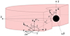Fig. 1. Geometry of the accreting matter around the BH. The fluid element is described by the radius vector, $\widehat{\mathit{r}}$, and velocity, $\widehat{\mathit{v}}$. Its trajectory is shifted from the midplane of the accretion disk by the angle, η. The observer is located in the direction of $\widehat{\mathit{o}}$, making an angle, i, with the disk normal, $\widehat{\mathit{n}}$.

$$\begin{array}{cc}\hfill \widehat{\mathit{n}}& =(0,0,1),\hfill \end{array}$$(1)

$$\begin{array}{cc}\hfill \widehat{\mathit{o}}& =(sini,0,cosi),\hfill \end{array}$$(2)

$$\begin{array}{cc}\hfill \widehat{\mathit{r}}& =(cos\phi cos\eta ,sin\phi cos\eta ,sin\eta ),\hfill \end{array}$$(3)

$$\begin{array}{cc}\hfill \widehat{\mathit{\phi }}& =(-sin\phi ,cos\phi ,0),\hfill \end{array}$$(4)

where η is the angle between the radius-vector, $\widehat{\mathit{r}}$, and the equatorial plane, φ is the azimuthal angle of the projection of $\widehat{\mathit{r}}$ to the x-y plane, measured from the x axis, and i is the inclination of the disk plane to the line of sight. The vectors, $\widehat{\mathit{r}}$ and $\widehat{\mathit{o}}$, form an angle, ψ:

$$\begin{array}{c}\hfill cos\psi \equiv \widehat{\mathit{r}}·\widehat{\mathit{o}}=sinicos\phi cos\eta +cosisin\eta .\end{array}$$(5)

Due to the effects of the light bending, the photons reaching the observer along $\widehat{\mathit{o}}$ are leaving the disk in the other direction, which we denote as ${\widehat{\mathit{k}}}_0$. Because the photon trajectories lie in a plane in the Schwarzschild metric, the wave vector, ${\widehat{\mathit{k}}}_0$, can be described by a linear combination of the radius-vector and the observer direction:

$$\begin{array}{c}\hfill {\widehat{\mathit{k}}}_0=[sin\alpha \widehat{\mathit{o}}+sin(\psi -\alpha )\widehat{\mathit{r}}]/sin\psi ,\end{array}$$(6)

where α is the angle between the radius vector and the direction toward the observer,

$$\begin{array}{c}\hfill cos\alpha \equiv \widehat{\mathit{r}}·{\widehat{\mathit{k}}}_0.\end{array}$$(7)

The angle, α, is related to ψ through the light-bending integral or an approximate light-bending formula (Pechenick et al. 1983; Beloborodov 2002; Poutanen 2020), introduced explicitly below. The wave vector makes an angle, ζ, with the disk normal,

$$\begin{array}{c}\hfill cos\zeta \equiv \widehat{\mathit{n}}·{\widehat{\mathit{k}}}_0=\frac{sin\alpha cosi+sin(\psi -\alpha )sin\eta }{sin\psi }.\end{array}$$(8)

Plasma orbits around the BH with Keplerian velocity and additionally gradually moves toward the compact object. The unit velocity vector is thus not purely parallel to the azimuthal vector. This deviation is described by the angle, σ, with respect to the equatorial radius vector, ${\widehat{\mathit{r}}}_{\mathrm{e}}=(cos\phi ,sin\phi ,0)$:

$$\begin{array}{c}\hfill cos\sigma \equiv {\widehat{\mathit{r}}}_{\mathrm{e}}·\widehat{\mathit{v}}.\end{array}$$(9)

We note that we did not consider vertical motion of matter (along the z axis). The unit velocity vector is described by

$$\begin{array}{c}\hfill \widehat{\mathit{v}}=(cos(\phi +\sigma ),sin(\phi +\sigma ),0).\end{array}$$(10)

Purely Keplerian rotation can be recovered by choosing σ = 90° or 270°; matter moves toward the BH for 90° < σ < 270°. For the magnitude of the dimensionless velocity, β = v/c, relative to the distant observer, we adopted the relation of Luminet (1979). In this work, we have considered the case in which the matter above the disk at a height of h = r sin η, where r = R/R_S is the circumferential radius measured in units of Schwarzschild radii, R_S = 2GM/c² (M is the mass of the compact object), and η ≠ 0, moves with Keplerian velocity corresponding to its equatorial radius, $r_{\mathrm{e}}=\sqrt{r^2-h^2}$. We have

$$\begin{array}{c}\hfill \beta =\frac{1}{\sqrt{2(r_{\mathrm{e}}-1)}}\end{array}$$(11)

and the Lorentz factor is then

$$\begin{array}{c}\hfill \gamma \equiv \frac{1}{\sqrt{1-{\beta }^2}}=\sqrt{\frac{r_{\mathrm{e}}-1}{r_{\mathrm{e}}-1.5}}.\end{array}$$(12)

The angle between the photon momentum and velocity vector is expressed as

$$\begin{array}{c}\hfill cos\xi \equiv \widehat{\mathit{v}}·{\widehat{\mathit{k}}}_0=\frac{sin\alpha }{sin\psi }sinicos(\phi +\sigma )+\frac{sin(\psi -\alpha )}{sin\psi }cos\eta cos\sigma .\end{array}$$(13)

Fast motions of matter close to the BH cause the photon trajectory to be altered by relativistic aberration. To account for this effect in the observed polarization properties, we considered quantities in a local fluid comoving frame. We denote quantities measured in this frame with primes. The photon vector in the comoving frame is

$$\begin{array}{c}\hfill {\widehat{\mathit{k}}}_0^{\prime }=\delta [{\widehat{\mathit{k}}}_0-\gamma \beta \widehat{\mathit{v}}+(\gamma -1)\widehat{\mathit{v}}(\widehat{\mathit{v}}·{\widehat{\mathit{k}}}_0)],\end{array}$$(14)

where δ is the Doppler factor,

$$\begin{array}{c}\hfill \delta \equiv \frac{1}{\gamma (1-\beta \widehat{\mathit{v}}·{\widehat{\mathit{k}}}_0)}=\frac{1}{\gamma (1-\beta cos\xi )}.\end{array}$$(15)

In the fluid frame, the photon makes an angle, ξ′, with the velocity vector,

$$\begin{array}{c}\hfill cos{\xi }^{\prime }\equiv \widehat{\mathit{v}}·{\widehat{\mathit{k}}}_0^{\prime }=\frac{cos\xi -\beta }{1-\beta cos\xi }=\gamma \delta (cos\xi -\beta ).\end{array}$$(16)

The angle between the photon momentum and the local normal in the disk is

$$\begin{array}{c}\hfill cos{\zeta }^{\prime }\equiv \widehat{\mathit{n}}·{\widehat{\mathit{k}}}_0^{\prime }=\delta cos\zeta .\end{array}$$(17)

To account for the light-bending effects and to transform the local emission and polarization to the observer frame, we need a relation between the angle, α, of the outgoing photon and the observer direction, ψ. We used the approximate relation (Poutanen 2020)

$$\begin{array}{c}\hfill cos\alpha \approx 1-(1-1/r)y\{1+\frac{y^2}{112r^2}-\frac{\mathrm{ey}}{100r}[ln(1-\frac{y}{2})+\frac{y}{2}]\},\end{array}$$(18)

where y = 1 − cos ψ. This relation gives accurate results given that the photon trajectories lie in the plane, which is strictly satisfied in the Schwarzschild metric. The transition from the Schwarzschild metric to the Kerr metric can be made by accounting for two additional effects: (i) a change in the orbital velocity profile and (ii) an additional twist in the light trajectories caused by the frame-dragging effects. While the former step is straightforward as the proper velocity profile is known, the latter effect is not accounted for by the present light-bending approximation. However, the second effect introduces deviations only for the trajectories that lie very close to the spinning BH, < 3R_S. Significant errors can be expected for the trajectories originating from the parts of the disk behind the BH (φ ∼ 180°) and a combination of a high spin parameter (a ≳ 0.8) and a high inclination (i ≳ 60°). At the same time, the integrated PD and PA in these cases show modest deviations (0.5% and 7°), becoming comparable to the observational uncertainties (Loktev et al. 2024). For the cases of prograde spins, a < 0.8, retrograde spins up to a = −1, and/or orbits at ∼3R_S or farther (comparable to the scales of the BH shadow probed by EHT), the current light-bending approximation leads to a precision that is higher than the observational errors.

The accretion flow is assumed to be optically thin to its own synchrotron emission and its spectral energy distribution follows the power-law dependence I_E ∝ E^−α_E. This means that the observer sees the whole volume of the flow, rather than its surface emission. To treat this, we split the accretion flow in surfaces in cylindrical coordinates, with the z axis being perpendicular to the equatorial plane of the accretion disk, and computed the total flux from each surface parallel to the equatorial plane by further splitting it into segments in the radial and azimuthal direction. The observed flux of each such segment depends on the solid angle it occupies on the sky (see more details in Poutanen & Beloborodov 2006; Loktev et al. 2022),

$$\begin{array}{c}\hfill \mathrm{d}\mathrm{\Omega }=\frac{\mathrm{d}Scos\zeta }{D^2}\mathcal{L}=\frac{R_{\mathrm{S}}^2}{D^2}\frac{r\mathrm{d}r\mathrm{d}\phi }{\sqrt{1-1/r}}\mathcal{L}cos\zeta ,\end{array}$$(19)

where the factor dScos ζ comes from the projection of the segment, D is the distance, and ℒ is the lensing factor (Beloborodov 2002; Poutanen 2020),

$$\begin{array}{cc}\hfill \mathcal{L}& \equiv \frac{1}{1-1/r}\frac{\mathrm{d}cos\alpha }{\mathrm{d}cos\psi }\approx \hfill \end{array}$$(20)

$$\begin{array}{cc}& \approx 1+\frac{3y^2}{112r^2}-\frac{\mathrm{e}y}{100r}[2ln(1-\frac{y}{2})+y\frac{1-3y/4}{1-y/2}].\hfill \end{array}$$(21)

The segment area projected onto the plane orthogonal to the photon propagation is the Lorentz invariant: dS′cos ζ′=dScos ζ. Hence, the observed solid angle can be expressed through the area of the disk segment as

$$\begin{array}{c}\hfill \mathrm{d}\mathrm{\Omega }=\frac{\delta \mathrm{d}{S}^{\prime }cos\zeta }{D^2}\mathcal{L}.\end{array}$$(22)

The latter expression will be used for computing the fluxes from the moving spots (blobs), for which the intrinsic area dS′ remains constant during the orbital motion. This area can be expressed through the comoving coordinates (r′,φ′) as (see also Nättilä & Pihajoki 2018; Bogdanov et al. 2019; Suleimanov et al. 2020)

$$\begin{array}{c}\hfill \mathrm{d}{S}^{\prime }=\frac{\gamma R_{\mathrm{S}}^2{r}_{\mathrm{e}}^{\prime }\mathrm{d}{r}_{\mathrm{e}}^{\prime }\mathrm{d}{\phi }^{\prime }}{\sqrt{1-1/r}}.\end{array}$$(23)

2.2. Transformation of polarized synchrotron emission

The magnetic field is described in the comoving frame, where it has radial, azimuthal, and vertical components. It is convenient to define the field through the components lying on the equatorial plane, B_eq, and along the disk normal, B_z. The equatorial field is further divided into the component lying along the gas motion and orthogonal to that, described by the angle, ϕ′, of the magnetic field direction relative to the gas motion. In the Cartesian coordinates of the comoving frame, the magnetic field vector is given by

$$\begin{array}{c}\hfill {\mathit{B}}^{\prime }=B_{\mathrm{eq}}[cos{\varphi }^{\prime }\widehat{\mathit{v}}+sin{\varphi }^{\prime }(\widehat{\mathit{n}}\mathbf{\times }\widehat{\mathit{v}})]+B_z\widehat{\mathit{n}}.\end{array}$$(24)

The unit vector, $\widehat{\mathit{B}}\prime \equiv \mathit{B}\prime /|\mathit{B}\prime |$, has components b_eq and b_z. The intensity and polarization of the photon depends on the angle between the magnetic field and photon direction,

$$\begin{array}{c}\hfill cos{\theta }^{\prime }\equiv {\widehat{\mathit{B}}}^{\prime }·{\widehat{\mathit{k}}}_0^{\prime }=b_{\mathrm{eq}}(cos{\varphi }^{\prime }cos{\xi }^{\prime }-\delta bsin{\varphi }^{\prime })+\delta b_{z}cos\zeta ,\end{array}$$(25)

where

$$\begin{array}{c}\hfill b=\frac{sin\alpha }{sin\psi }sinisin(\phi +\sigma )+\frac{sin(\psi -\alpha )}{sin\psi }cos\eta sin\sigma .\end{array}$$(26)

The radiation field in the comoving frame can be generally described by the Stokes vector,

$$\begin{array}{c}\hfill {\mathit{I}}_{E^{\prime }}^{\prime }({\theta }^{\prime })\equiv \left[\begin{array}{c}{I}_{E^{\prime }}^{\prime }\\ Q_{E^{\prime }}^{\prime }\\ U_{E^{\prime }}^{\prime }\end{array}\right]=I_{E^{\prime }}^{\prime }\left[\begin{array}{c}1\\ P_{\mathrm{s}}(E^{\prime })cos2{\chi }_0\\ P_{\mathrm{s}}(E^{\prime })sin2{\chi }_0\end{array}\right],\end{array}$$(27)

where I_E′′ is the local rest-frame specific intensity, P(E′) corresponds to the PD in this frame, and χ₀ gives the PA relative to the chosen axis. A natural choice for synchrotron emission is the axis going along the magnetic field vector. The basis vectors are

$$\begin{array}{c}\hfill {\widehat{\mathit{e}}}_1=\frac{{\widehat{\mathit{B}}}^{\mathbf{\prime }}-cos{\theta }^{\prime }{\widehat{\mathit{k}}}_0^{\prime }}{sin{\theta }^{\prime }},{\widehat{\mathit{e}}}_2=\frac{{\widehat{\mathit{k}}}_0^{\prime }\times \widehat{{\mathit{B}}^{\mathbf{\prime }}}}{sin{\theta }^{\prime }}.\end{array}$$(28)

In this basis, χ₀ = 90° and synchrotron emission and polarization can be expressed as

$$\begin{array}{c}\hfill {\mathit{I}}_{E^{\prime }}^{\prime }({\theta }^{\prime })=c_0{E}^{\prime -{\alpha }_E}{l}_{\mathrm{ph}}^{\prime }{(Bsin{\theta }^{\prime })}^{1+{\alpha }_E}\left[\begin{array}{c}1\\ -P_{\mathrm{s}}\\ 0\end{array}\right],\end{array}$$(29)

where c₀ is a constant (e.g., Eq. (6.36) in Rybicki & Lightman 1979), l_ph′ is the photon path length through the synchrotron-emitting medium (measured in the comoving frame), and P_s = (p + 1)/(p + 7/3) gives the PD of the power-law electrons with index p = 2α_E + 1 (Ginzburg & Syrovatskii 1965). The typical value considered for the optically thin synchrotron emission is α_E = 0.7, while the observations of bright flares in Sgr A^* tend to give a somewhat steeper slope, α_E ≈ 1 (Gillessen et al. 2006). The latter value was used in the modeling of the Sgr A^* and M87^* (Narayan et al. 2021; Vincent et al. 2024), and we adopted this value for the calculations presented in this work. The advantage of such a representation of the observed Stokes parameters is that it explicitly distinguishes the PA from the PD. The PD is a Lorentz invariant; hence, the transformation of polarization signatures reduces to the tracing of the changes in the photon electric field orientation (as a result of aberration and light bending) along the photon trajectory.

The intensity of the steady matter flow in the comoving frame is related to the observed intensity as

$$\begin{array}{c}\hfill I_E=g^3{I}_{E^{\prime }}^{\prime }\propto g^{3+{\alpha }_E}{E}^{-{\alpha }_E},\end{array}$$(30)

where $g\equiv E/E\prime =\delta \sqrt{1-1/r}$ is the total redshift factor (Luminet 1979; Chen & Shaham 1989) and the latter expression corresponds to the power-law spectrum I_E′′∝E′^−α_E. The photon path can be expressed as

$$\begin{array}{c}\hfill l_{\mathrm{ph}}^{\prime }=g{l}_{\mathrm{ph}}=\frac{h_0}{{\widehat{k}}_0^{{\prime }^{(z)}}}=\frac{h_0}{cos{\zeta }^{\prime }},\end{array}$$(31)

where h₀ is the characteristic vertical thickness of each synchrotron-emitting layer in the disk, seen in the observer’s frame, and ${\widehat{k}}_0^{\prime (z)}$ is the z component of the photon momentum vector in the comoving frame.

The observed flux from a segment of the disk is related to the observed intensity of radiation as

$$\begin{array}{c}\hfill \mathrm{d}{F}_E=I_E\mathrm{d}\mathrm{\Omega }=\delta I_E\mathcal{L}cos\zeta \frac{\mathrm{d}{S}^{\prime }}{D^2}.\end{array}$$(32)

Stokes parameters (in flux units) of each layer in the disk were obtained by integrating over the equatorial radii and azimuthal coordinates.

$$\begin{array}{cc}\hfill {\mathit{F}}_E& \equiv \left[\begin{array}{c}{F}_I(E)\\ F_Q(E)\\ F_U(E)\end{array}\right]=\int \mathrm{d}\mathrm{\Omega }\left[\begin{array}{c}{I}_E\\ Q_E\\ U_E\end{array}\right]=\hfill \\ & =\int \mathrm{d}\mathrm{\Omega }{g}^3\mathbf{M}(r,\phi ){\mathit{I}}_{E^{\prime }}^{\prime }({\theta }^{\prime })=\hfill \\ \hfill & =\int \frac{\mathrm{d}{S}^{\prime }}{D^2}{g}^3\delta \mathcal{L}cos\zeta \mathbf{M}(r,\phi ){\mathit{I}}_{E^{\prime }}^{\prime }({\theta }^{\prime }),\hfill \end{array}$$(33)

where the transformation from the vector, I′_E′(θ′), to the observed Stokes vector was done through the rotation Mueller matrix,

$$\begin{array}{c}\hfill \mathbf{M}(r,\phi )=\left[\begin{array}{ccc}1& 0& 0\\ 0& cos2{\chi }^{\mathrm{tot}}& -sin2{\chi }^{\mathrm{tot}}\\ 0& sin2{\chi }^{\mathrm{tot}}& cos2{\chi }^{\mathrm{tot}}\end{array}\right].\end{array}$$(34)

Here, χ^tot corresponds to the total rotation of the polarization (Stokes) vector from the comoving frame to the observer’s frame. For the synchrotron emission of the power-law electrons, the expression in Eq. (33) can be simplified to

$$\begin{array}{cc}\hfill {\mathit{F}}_E& =f_{E,0}\int \mathrm{d}\mathrm{\Omega }\frac{g^{3+{\alpha }_E}}{\delta cos\zeta }{(sin{\theta }^{\prime })}^{1+{\alpha }_E}\left[\begin{array}{c}1\\ -P_{\mathrm{s}}cos2{\chi }^{\mathrm{tot}}\\ -P_{\mathrm{s}}sin2{\chi }^{\mathrm{tot}}\end{array}\right]=\hfill \\ \hfill & =f_{E,0}\int \int \frac{\gamma R_{\mathrm{S}}^2{r}_{\mathrm{e}}^{\prime }\mathrm{d}{r}_{\mathrm{e}}^{\prime }\mathrm{d}{\phi }^{\prime }}{\sqrt{1-1/r}}{g}^{3+{\alpha }_E}\mathcal{L}{(sin{\theta }^{\prime })}^{1+{\alpha }_E}\left[\begin{array}{c}1\\ -P_{\mathrm{s}}cos2{\chi }^{\mathrm{tot}}\\ -P_{\mathrm{s}}sin2{\chi }^{\mathrm{tot}}\end{array}\right],\hfill \end{array}$$(35)

where f_E, 0 = c₀h₀E^−α_EB^1 + α_E. In the latter representation, we have preserved the expression of dS′, as it is most useful for moving spots, while the former expression is useful for calculations of the synchrotron-emitting disk image. Below, we have also used the relative Stokes parameters, obtained as q = F_Q(E)/F_I(E) and u = F_U(E)/F_I(E). The developed formalism can be used to construct the spectro-polarimetric images (see also Loktev et al. 2022, 2024). For this, we introduced the Cartesian coordinates, X and Y, in the plane of the sky, scaled to units of R_S, as

$$\begin{array}{c}\hfill \left[\begin{array}{c}X\\ Y\end{array}\right]=b\left[\begin{array}{c}-sin\mathrm{\Phi }\\ cos\mathrm{\Phi }\end{array}\right]=\frac{r}{\sqrt{1-1/r}}\frac{sin\alpha }{sin\psi }\left[\begin{array}{c}sin\phi cos\eta \\ sinisin\eta -cosicos\phi cos\eta \end{array}\right].\end{array}$$(36)

Here, Φ corresponds to the position angle of the point in the plane of the sky, measured counterclockwise from the projection of the disk axis on the sky, and $b=rsin\alpha /\sqrt{1-1/r}$ corresponds to the impact parameter.

2.3. Rotation of polarization angle

The method described above allowed us to compute the observed Stokes parameters once the total rotation of the polarization plane along the photon trajectory (χ^tot) was known. The PA seen by the observer (with respect to the direction of the disk axis) was computed as a sum of the PA of emitted photon and its total rotation:

$$\begin{array}{c}\hfill \chi ={\chi }_0+{\chi }^{\mathrm{tot}},\end{array}$$(37)

where χ₀ = 90° for synchrotron emission. Under the assumption of photon trajectories lying in plane (corresponding to the Schwarzschild metric), the total rotation can be presented as the sum of rotations caused by the light-bending and relativistic aberration effects (the aberration effects need to be computed in the curved space, i.e., accounting for the deflection of the photon path, which is different from the case of the flat space Pineault 1977; Loktev et al. 2022). We followed the methodology described in Loktev et al. (2022, 2024), in which the rotation angles were computed relative to the normal of the disk (in our case, the equatorial plane). As the PA of synchrotron radiation is related to the magnetic field direction, we first need to link this direction to the disk normal via the rotation angle, χ^B. Then, the rotation of polarization plane resulting from light bending is described by the angle χ^GR and the special relativity (aberration) effects are accounted for by the angle χ^SR. This leads to the total rotation angle through the sum

$$\begin{array}{c}\hfill {\chi }^{\mathrm{tot}}={\chi }^B+{\chi }^{\mathrm{GR}}+{\chi }^{\mathrm{SR}}.\end{array}$$(38)

The explicit expression for the rotation caused by the effects of special relativity is given in Appendix A:

$$\begin{array}{c}\hfill tan{\chi }^{\mathrm{SR}}=-\beta \frac{cos\alpha cos\zeta }{{sin}^2\zeta -\beta cos\xi }.\end{array}$$(39)

The form of this expression is the same as in Eq. (31) of Loktev et al. (2022); however, the terms are not the same. Namely, in this work we explicitly considered the cases of a nonzero accretion velocity (σ ≠ 90° or 270°) and an out-of-equatorial-plane matter location (η ≠ 0); hence, the expressions for the terms cos ζ, sin ζ, and cos ξ are generally different from the ones given in the former work (see Eqs. (8) and (13)). In the case of the flat (Minkowski) space, the expression reduces to

$$\begin{array}{c}\hfill tan{\chi }_{\mathrm{flat}}^{\mathrm{SR}}=-\beta tani\frac{sinicos\phi cos\eta +cosisin\eta }{sini-\beta cos(\phi +\sigma )}.\end{array}$$(40)

For η = 0 and σ = 90°, it reduces to Eq. (32) of Loktev et al. (2022).

The expression for χ^GR becomes lengthy once we consider photons originating from the plane that is not equatorial. In coordinate form, it reads as (see Appendix A)

$$\begin{array}{c}\hfill tan{\chi }^{\mathrm{GR}}=cos\eta \frac{{\tilde{a}}_{1}sin\psi -{\tilde{a}}_{2}sinisin\phi }{{\tilde{a}}_1{\tilde{a}}_2-{cos}^2\eta {sin}^{2}i{sin}^2\phi sin\alpha },\end{array}$$(41)

where

$$\begin{array}{cc}\hfill {\tilde{a}}_1& =sin\eta +cot\psi sinicosisin\alpha sin\phi ,\hfill \end{array}$$(42)

$$\begin{array}{cc}\hfill {\tilde{a}}_2& =sin\alpha [cos\alpha cosi-sin\eta cos(\psi -\alpha )].\hfill \end{array}$$(43)

For η = 0, this expression reduces to Eq. (29) of Loktev et al. (2022).

The rotation angle transforming the polarization direction from the local magnetic field direction relative to the disk normal can be expressed as (see Appendix A)

$$\begin{array}{c}\hfill {\chi }^{\mathrm{B}}=arctan\left(\frac{{\widehat{\mathit{k}}}_0^{\prime }·(\widehat{\mathit{n}}\times \widehat{{\mathit{B}}^{\mathbf{\prime }}})}{\widehat{\mathit{n}}·\widehat{{\mathit{B}}^{\mathbf{\prime }}}-({\widehat{\mathit{k}}}_0^{\prime }·\widehat{\mathit{n}})({\widehat{\mathit{k}}}_0^{\prime }·\widehat{{\mathit{B}}^{\mathbf{\prime }}})}\right).\end{array}$$(44)

The expression for χ^B takes into account both the light-bending effects (ψ ≠ α) and the Lorentz transformation of the magnetic field (primed quantities). This angle is related to both general and special relativity effects, and depends on α and δ. The explicit expression for the angle χ^B reads as

$$\begin{array}{c}\hfill tan{\chi }^B=\frac{[\tilde{b}cos{\varphi }^{\prime }+\gamma sin{\varphi }^{\prime }(cos\xi -\beta )]}{\delta cos\zeta [\gamma cos{\varphi }^{\prime }(cos\xi -\beta )+\tilde{b}sin{\varphi }^{\prime }]+\frac{b_z}{b_{\mathrm{eq}}}[\delta {cos}^2\zeta -\frac{1}{\delta })]},\end{array}$$(45)

where $\stackrel{\sim }{b}$ is taken from Eq. (26).

The expression for χ^B for purely circular rotation (σ = 90°) in the equatorial plane (η = 0), far from the compact object (γ → 1, β → 0) and small, yet nonzero inclinations (i → 0), reduces to

$$\begin{array}{cc}\hfill tan{\chi }^B& \approx tan\phi ,\mathrm{if}{\varphi }^{\prime }=90°,\hfill \\ \hfill tan{\chi }^B& \approx -cot\phi ,\mathrm{if}{\varphi }^{\prime }=0.\hfill \end{array}$$(46)

Hence, we obtain

$$\begin{array}{cc}\hfill {\chi }^B& \approx \phi \mathrm{for}\mathrm{the}\mathrm{radial}\mathrm{field},\hfill \\ \hfill {\chi }^B& \approx \phi -90°\mathrm{for}\mathrm{the}\mathrm{toroidal}\mathrm{field}.\hfill \end{array}$$(47)

The observed PA is then χ = φ + 90° for the radial field and χ = φ for the toroidal one, and in both cases the result matches the intuitive expectations.

3. Results

The developed formalism allowed us to analytically compute the polarimetric signatures of matter close to the event horizon. The power of such a formalism is that we can separately understand each effect contributing to the total modification of polarization, and hence develop an intuition about the range of the model parameters for the given observed set of data. Furthermore, using the developed formalism, we can compare the predictions of the polarization rotation to the synchrotron source in an orbit around the BH.

Many parameters affect the polarimetric properties of the synchrotron source: distance to the BH, r, B-field topology, observer inclination, i, the location of the source with respect to the disk plane, η, and the direction of velocity vector determined by σ. Generally, with increasing distance to the BH, r, all relativistic effects fade and only the topology of the magnetic field affects the PA for different parts of the disk. Other effects are discussed below in detail. To produce the figures, we have considered the point source at given coordinates, unless stated otherwise.

3.1. Rotation of polarization angle due to relativistic effects

To disentangle the rotation of the polarization plane caused by relativistic effects from the effect of the B-field orientation changes, we first considered the case of a vertical field, B = (0, 0, B_z). In the absence of the relativistic effects, this case is trivial: the PA is constant and equal to 90° (for all inclinations except for the degenerate i = 0). In the absence of relativistic effects, which can alter the direction of the magnetic field, the angle is the same across the entire disk. We verified that our calculations reproduce this value with high accuracy.

We then included the special and general relativistic effects; we show the contours of constant PA as a function of the disk coordinates (r, φ) in Fig. 2. We assumed circular counterclockwise rotation, σ = 90°, and considered different inclinations, i = 30°, 60°, and 80°, and various elevations above the disk plane, η = 0, ±20°. We note that the cases η ≠ 0 correspond to conical surfaces above or below the disk plane, but very similar contours can be obtained by fixing the height to h = 3tanη for all radii. All of the parameters are listed in Table A.1. The azimuthal angle in the disk grows from the direction (X, −Y). For the case of rotation in the equatorial plane (η = 0) the contours of χ^GR + χ^SR are essentially the same as the ones shown in Fig. 4 of Loktev et al. (2022). We note the presence of a critical point at i = 30° near coordinates ( − 3, 2), where all lines of constant PA rotation intersect. This point corresponds to the place in the disk that an observer sees face-on as a result of the light-bending and SR effects; hence, PD = 0 at this point, leading to a degeneracy of PA.

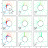Fig. 2. Contours of PA rotation (χSR + χGR) for different i = 30°, 60°, and 80° and η = 0, ±20° in the disk coordinates (r, φ), where r is measured in units of Schwarzschild radii. Azimuth increases in the counterclockwise direction, as is shown by the arrow in panel (a). Numbers on the contours correspond to the rotation angle (in degrees). The thick red line without a mark corresponds to ±90° rotation. Matter is assumed to have a purely circular Keplerian velocity in the counterclockwise direction (σ = 90°). The dashed line indicates the location of the ISCO. Contours corresponding to η = 0 (upper row) match those shown in Loktev et al. (2022). The effects of matter elevation above (or below) the orbital plane are clearly visible when comparing to the case of in-plane rotation. If matter is located in front of the BH (middle row), for the same radius from the BH the GR and SR effects appear to be less pronounced.

Movement around the origin in Fig. 2 corresponds to a rotation of a point (infinitely small spot) in a disk at a certain radius. The radius containing the critical point separates the region where the rotation of the PA crosses the ±90° cycle point from the region where the PA does not make a cycle. These two regions correspond to either one or two loops made by Stokes parameters per one orbital cycle of a spot, and the existence of such critical point has previously been noticed in a number of works (e.g., Dovčiak et al. 2008; GRAVITY Collaboration 2018, 2020b; Gelles et al. 2021; Vos et al. 2022; Loktev et al. 2022; Vincent et al. 2024).

The location of a critical point has been discussed in detail in Vincent et al. (2024) under the assumption of Minkowski space. However, its appearance is not entirely caused by aberration effects, and there are essential differences with respect to the contour morphology in the Schwarzschild metric. First, the SR rotation itself is different in the Minkowski and Schwarzschild metric (compare Eqs. (39) and (40)), as the ${\widehat{\mathit{k}}}_0$ and $\widehat{\mathit{o}}$ directions are not aligned. Inclusion of the light bending within the calculation of the PA rotation caused by aberration mainly leads to a strong up-down contour asymmetry (around the horizontal line, y = 0, in Fig. 2) and a shift in the position of the critical point from the azimuth, φ = 270°, for flat space toward φ ≈ 230° for the Schwarzschild space.

Interestingly, pure aberration effects in the Schwarzschild metric can lead to a formation of two critical points at different radii (Fig. 6 in Loktev et al. 2022); however, the additional rotation due to light-bending effects alters their location and may lead to a shift of one of them below ISCO. This effect is seen in Fig. 2: only one critical point is observed in the panels (a), (d), and (g), corresponding to i = 30°. At higher inclinations, the critical point disappears because the joint action of aberration and light-bending effects are not strong enough to direct the photons escaping vertically from the disk into the observer’s direction, and hence the PA rotation is always smaller than one complete cycle.

The radius and azimuthal coordinate of the critical point, along with the contour morphology, is also altered if the matter is located above or below the equatorial plane (middle and lower panels in Fig. 2). Since in our assumptions we considered the same speed of matter at different elevations, the effect purely scales with the magnitude of light bending.

3.2. Effects of magnetic field orientation

Additional rotation of PA can be gained because of the varying orientation of magnetic field with the azimuth; for example, in the cases of purely toroidal and radial magnetic fields. In Fig. 3, we show the results of calculations of χ^B, as a function of the disk azimuth, φ, for these two cases and three different inclinations of the observer: i = 30°, 60°, and 80°. Circular counterclockwise (σ = 90°) rotation of matter at the equatorial plane of the disk (η = 0) is assumed. All of the parameters are listed in Table A.1. Different lines correspond to matter located at different equatorial radii: r_e = 3 (solid black), 5 (dashed red), 15 (dash-dotted green) and 50 (dotted blue).

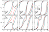Fig. 3. Rotation of PA due to magnetic field orientation, as a function of azimuth (in disk coordinates) for different equatorial radii (measured in units of Schwarzschild radii): re = 3 (solid black), 5 (dashed red), 15 (dash-dotted green), and 50 (dotted blue). The matter is assumed to undergo circular, counterclockwise rotation (σ = 90°) with velocity following Luminet’s law. The upper panels correspond to a purely radial comoving magnetic field (ϕ′ = 90°) and the lower panels correspond to a purely toroidal field (ϕ′ = 0). The columns (left to right) correspond to the observer inclination, i = 30°, 60°, and 80°.

For radii of r_e ≳ 50, the angle makes two full loops per azimuthal cycle for any inclination. In the simplest case of the disk at a relatively low inclination, i = 30°, the rotation, χ^B, increases with the azimuth nearly linearly. This replicates the behavior for small inclinations and large distances to the compact object described in Eq. (47).

For radii of r_e ≲ 5, there are noticeable deviations from the behavior at large radii thanks to the pronounced effects of relativistic aberration, modified by the light bending. The difference is particularly great at an azimuth of φ ∼ 270°; that is, for the approaching side of the disk. For i = 30°, the changes are severe, as rotation reduces to one loop over the azimuthal cycle, and hence the whole topology of rotation changes. The behavior of the PA with the azimuth is now different for the radial and toroidal fields, making it potentially possible to distinguish these fields via orbital (azimuthal) phase-resolved polarimetric data.

For both the toroidal and radial fields, the total PA rotation (χ^tot) is dominated by the rotation caused by the different magnetic field orientation (χ^B), rather than the rotation caused by relativistic effects (χ^GR + χ^SR), and the contours of constant rotation do not contain the critical point (examples of contours for the case of the toroidal field and different i are shown in Fig. 4). However, the lines of PA rotation have nearly the same morphology for pure radial and toroidal fields, albeit shifted in azimuth. Hence, their linear combination may lead to a substantial reduction of the PA rotation with the azimuth, essentially mimicking the vertical field, and may replicate the behavior near the critical point (Fig. 2). We find that the critical point appears, for example, for the combination of radial and toroidal field components (ϕ′ = 45°) at high inclinations (i = 80°) and matter below the equatorial plane (η = −20°).

Fig. 4. Contours of constant total rotation angle (χtot) for the case of a toroidal magnetic field (σ = 90°, ϕ′ = 0) and the equatorial plane matter movement, in disk coordinates. We note the disappearance of the critical point, compared to the case of a vertical field, as the rotation is dominated by the changing magnetic field orientation (χB). The observed PA, χ, was obtained by adding χ0 = 90°.

3.3. Effects of non-equatorial motion

The GR and SR effects on rotation of polarization plane have been studied, using the aforementioned formalism, in the case of razor-thin matter in an equatorial plane of BHs (Loktev et al. 2022, 2024). Emitting matter may, however, be elevated above the equatorial plane in the case of geometrically thick disks or if emission arises at the interface between the inflow and outflow (edge-brightened jet found, e.g. in high-resolution images of Cen A, Janssen et al. 2021). Our formalism enables a direct comparison between the polarization rotation for the matter rotating in the plane containing the BH itself (equatorial plane, η = 0) and that of the matter elevated by the height, h (set by η ≠ 0) above or below this plane.

In Fig. 5, we show the resulting observed PA (χ) for the specific case of η = 20°. The topology of the lines is the same as for the case η = 0, but the absolute values differ. In the cases of the equatorial field (two upper rows of panels), the PA rotation is dominated by the χ^B term and GR and SR effects are less pronounced, as lines corresponding to different radii nearly overlap, especially for smaller inclinations. Figure 2 (d-f) shows this effect in more detail. The contours of the same χ^GR + χ^SR are generally closer to the event horizon for η = 20°, compared to η = 0. This means that for the same distance from the BH, the polarization plane rotation is more severe for the case of equatorial rotation than for the matter located between this plane and the observer. The main reason for this is that for higher η, a smaller part of photon path lies close to the strong gravitational field of the BH; hence, bending effects are less pronounced. Likewise, if the matter is located below the equatorial plane – that is, behind the BH – relativistic effects become most pronounced and contours of higher PA rotation appear (Fig. 2g-i).

Fig. 5. PA seen by the observer (χ) obtained for the angle η = 20°, for different radii, observer inclinations, and magnetic fields, as a function of the azimuth in the disk. The upper panels show the case of the radial field, the middle panels correspond to the purely toroidal field, and the lower panels correspond to the vertical field. The columns correspond, from left to right, to an increasing observer inclination: i = 30°, 60°, and 80°. The matter is assumed to rotate counterclockwise (σ = 90°), with a velocity following Luminet’s law.

To quantify the effects of matter elevation at different radii, in Fig. 6 we show the difference between the total rotation (χ^tot) for the case of η = 20° with respect to the case η = 0 for various inclinations and magnetic field configurations, observer inclinations, and radii to the BH. For large distances, r, the effect of elevated matter is minor, as was expected. However, for distances of r ≲ 10, the difference can reach 30°, becoming comparable to the total rotation, and hence cannot be neglected. The difference can reach 90° for certain parameters and azimuths. It is generally asymmetric with respect to φ and has a complex dependence on the magnetic field orientation, making it difficult to a priori predict the effect of elevated matter on the PA rotation. However, it is generally clear that the effect is highest at azimuths of 180 ≲ φ ≲ 270, where the GR and SR effects are most pronounced. Since these effects strongly depend on the distance to the compact object and matter velocity, any changes to the distance caused by nonzero elevation result in substantial changes to the total PA rotation.

Fig. 6. Difference between the PA obtained for the angle η = 20° and η = 0 (χtot(η = 20° ) − χtot(η = 0)), for different radii, observer inclinations, and magnetic fields, as a function of the azimuth in the disk coordinates. The upper panels show the case of the radial field, the middle panels correspond to the purely toroidal field, and the lower panels correspond to the vertical field. The columns, from left to right, correspond to an increasing observer inclination: i = 30°, 60°, and 80°. The matter is assumed to rotate counterclockwise (σ = 90), with a velocity following Luminet’s law.

3.4. Effects of noncircular motion

Accretion flows around BHs have a nonzero radial velocity component – the accretion speed. In our formalism, this is parameterized by the angle, σ, which may potentially affect the resulting rotation of polarization, as the highest aberration may be achieved at a different angle. The trivial case of changing direction is the clockwise rotation, σ = 270°, which can be visualized by simply changing the azimuthal angle, φ_cl − w = 360° −φ. Another important example includes spherical (Bondi-Hoyle) accretion, σ = 180°. We consider the effects of noncircular motions of matter for different magnetic field geometries and varying inclinations in Fig. 7.

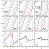Fig. 7. Effects of noncircular motion (σ) on the observed PA (χtot) for different inclinations (left to right: i = 30°, 60°, and 80°) and magnetic fields (upper panels: radial field, middle panels: toroidal field, lower panels: vertical field), as a function of the azimuth in the disk coordinates. Different directions of motion correspond to σ = 90° (solid black lines), 110° (dashed red), 150° (dash-dotted green), and 180° (dotted blue). The emitting matter is assumed to be located in the equatorial plane (η = 0) at a distance of r = 5, with a dimensionless velocity obeying Luminet’s law.

In equatorial field cases (panels a–f), the field direction is always fixed either parallel or orthogonal to the matter motion, and hence when the velocity direction changes, the field direction follows, introducing constant shifts to the lines. Apart from the constant shifts, there are minor deviations of the PA dependence on the azimuthal angle owing to the different combined SR and GR effects. Again, these are mostly pronounced for the locations of matter behind the BH (φ ∼ 180°).

In the case of the vertical field, the changes are generally likewise minor (Fig. 7h,i). The highest difference with respect to the default counterclockwise rotation occurs for i = 30° (Fig. 7g), close to the location of the critical point. By changing the velocity vector, it is possible to shift this point, changing the character of the PA rotation from the limited range (solid black line in Fig. 7g) to two complete loops per orbit (dashed red, dash-dotted green, and dotted blue). Hence, the σ parameter may be degenerate with inclination.

4. Applications

In this section, we compare the topology of static and dynamic signatures of BHs. The developed formalism can be applied to reproduce the horizon-scale images and polarimetric properties of M87* and Sgr A* (Event Horizon Telescope Collaboration 2019, 2021, 2022, 2024a), as well as dynamic polarimetric signatures of Sgr A* (Wielgus et al. 2022; GRAVITY Collaboration 2023). We start with the expected polarimetric signatures of the orbiting compact and extended spots. We then discuss polarimetric signatures of the narrow disk ring. After that, we show examples of computed images of the geometrically thick accretion disk.

4.1. Hot spot rotation

The quiescent level of Sgr A* accretion is known to be interrupted by the bright flares, when the observed radio (submillimeter) and NIR fluxes can suddenly increase by 1–2 orders of magnitude (e.g. Baganoff et al. 2001; Genzel et al. 2003). The characteristic timescales of the flares are roughly consistent with Keplerian time close to the event horizon, and the hot spot rotation scenario was proposed to explain the flares (Broderick & Loeb 2006; Trippe et al. 2007). Alternatively, a pattern movement could be responsible for the production of similar characteristics (Matsumoto et al. 2020; Aimar et al. 2023). Recently, observed movement of the brightness centroid and loops of polarized fluxes have given additional support to these scenarios (GRAVITY Collaboration 2018; Wielgus et al. 2022; GRAVITY Collaboration 2023). Perhaps the most intriguing property found in those data is the one observed polarimetric loop in Stokes parameters per one orbital period, with a zero-polarization point (where absolute Stokes parameters Q  =  U  =  0) being located within this loop (in the NIR, where interstellar polarization is expected to be low). Moreover, the PA was found to change at a nearly constant rate as a function of time, presumably corresponding to the azimuthal angle in the accretion disk (GRAVITY Collaboration 2023).

One complete rotation of PA per orbit is not expected to appear for a large fraction of the parameter space and is tightly linked to the location of the critical point (where the observed polarization turns zero). If the orbit does not intersect the location of a critical point (r_cr, φ_cr), either two complete loops of Stokes parameters (for orbits within r_cr) or one loop that does not enclose the origin Q = U = 0 (orbits beyond the radius of the zero-polarization point) are generally expected (see Sect. 3.1). The appearance of the critical point is also tightly related to the magnetic field direction (Sect. 3.2): if the spot is moving in the equatorial plane, the critical point is only observed in the case of the vertical field B = B_z. In order to reproduce the observed topology, the radius and inclination of the hot spot should clearly coincide with the location of the critical point, so that the second loop, which occupies a small fraction of the orbital motion, is small or completely absent, and the rotation around the secondary loop is fast enough to not affect the constant rate of PA changes. In other words, for the data that are limited in time and angular resolution, it should not be feasible to resolve the movement along the second polarimetric loop.

The limited range of radii and inclinations for which the critical point exists, as well as the strong dependence on the magnetic field topology, then translates into highly constraining estimates on these parameters that come from polarimetry (e.g., GRAVITY Collaboration 2018, 2023). In Fig. 8, we show the contours of PA rotation for the case of the vertical field, with inclinations over 90° that are believed to be relevant to the accreting matter around Sgr A*. For the inclinations outside 140° < i < 165°, the location of the critical point is either outside of the ∼10R_S, corresponding to scales that the instruments are sensitive to, or within the ISCO.

Fig. 8. Contours of constant GR and SR rotation angles (χGR + χSR), in disk coordinates. The position of the critical point is shown as a function of inclination for rotation caused solely by GR and SR effects (equivalent to B = Bz). The disk rotates counterclockwise (σ = 90°) in the equatorial plane, but at inclinations of i = 165° (a), 155° (b), and 140° (c) it is seen as rotating in the clockwise direction.

In Fig. 9, we show the patterns traced by the spot rotating in the equatorial plane. Increasing time (or azimuth) is shown as saturating color: the pale part of the curves corresponds to the beginning of the rotation from φ = 0. To produce this figure, we used the latter representation of (Stokes) fluxes in Eq. (35), and kept dS′=const throughout the rotation. While Eq. (35) was derived assuming the spot emits through the upper surface of the disk, the same expression is also valid for the synchrotron emission from a spherical, optically thin spot of radius h₀, as in this case the factors, cos ζ, entering the area, dS′, and the photon path, l_ph′, are omitted.

Fig. 9. Flux Stokes parameters, FQ and FU, obtained using η = 0, for different radii, B and i. Keplerian velocity and σ = 90° are assumed (note that for the considered inclinations, the observed matter movement is clockwise on the sky). Increasing saturation of color corresponds to progression of the spot along the azimuth. The time when the line intersects zero PD corresponds to the passage through the critical point. Note different scales in figures.

The loop topology becomes altered if the matter gradually rises above or below the equatorial plane. This scenario is expected; for example, if the spots correspond to ejecting plasmoids (Aimar et al. 2023). We illustrate this case by assuming a gradual increase in matter elevation above the orbital plane, keeping the equatorial radius of matter the same (helical motion). The results of calculations for the case of the vertical magnetic field and different inclinations are shown in Figs. 10 and 11. The topology of the loops strongly depends on the azimuthal angle, φ₀, at which the spot starts rising, as is evident from the comparison of the top, middle, and bottom panels.

Fig. 10. Stokes parameters, U and Q, for matter flying toward the observer (ηmax = 45°), in the direction orthogonal to rotation plane, at different launching azimuthal angles: φ0 = 90° (upper panels), 180° (middle panels), and 270° (lower panels). Note different scales in panels.

Next, we considered the behavior of relative Stokes parameters in the regime of strong gravity and fast motions. The PD is Lorentz-invariant, and hence compact spots located in any part of the disk are expected to have the PD that corresponds to the PD of intrinsic emission from the corresponding disk segment viewed at an angle, ζ′. Angular dependence of the intrinsic PD, for example in the case of the optically thick disk atmospheres, leads to a modulation of the PD with orbital phase, since the viewing angle, ζ′, for a given observer’s inclination and radius, changes with the azimuth (e.g., Fig. 7 of Loktev et al. 2022). However, in the case of the synchrotron emission, the PD does not depend on the viewing angle, but only on the index of the power-law electrons (Ginzburg & Syrovatskii 1965). Hence, in the simple scenario, we do not expect changes in the PD with the orbital phase (azimuth), which translates into the topology of two complete cycles or a part of the cycle pattern in the qu plane. In the lower panels of Fig. 12, we show the direct calculation of the relative Stokes parameters in the case of an infinitely small spot at different radii and inclinations (black, red, and green curves) that confirm the two-cycle or part-cycle pattern. A more complex pattern may be obtained if the angular dependence of the PD is caused by the angular-dependent (with respect to the magnetic field orientation) electron spectral index, p.

4.2. Polarimetry of an extended spot and disk ring

An important property of the observed signal is the considerably lower PD detected in the flares, ∼25%, as compared to the theoretical expectations, ∼70%. The reduction in the PD may be caused by the beam depolarization (Narayan et al. 2021), or if the spot is extended in the azimuthal, vertical, and/or radial direction (see examples of simulations in Yfantis et al. 2024). In Fig. 12, we compare the absolute (F_Q, F_U) and relative (q, u) Stokes parameters for the infinitely compact spot (black, red, and green curves) to those that are averaged in the azimuthal direction (infinitely thin disk segment), assuming the spot size of a quarter circle (blue, violet, and yellow curves). The spot is assumed to move and each point in the plot corresponds to the azimuth of the middle of the spot. The depolarization essentially occurs because of the averaging over Stokes vectors with different angles, but a large spot size (comparable to the orbital scale) is needed. The single loop and distorted shapes of the qu parameters can be recovered.

It is noteworthy that the behavior of NIR polarization during the flares does not always follow the one-loop pattern over the ∼70 min timescale (thought to correspond to the orbital period of the spots). Namely, the pattern detected in flares from August 18, 2019, and May 19, 2022 (Fig. 1 of GRAVITY Collaboration 2023), resembles a line rather than a loop. Furthermore, simultaneous high-precision astrometric measurements available for the flare on May 19, 2022, do not resemble a circle, expected for the circular motion around the compact object, but likewise are more consistent with a line. Similar behavior is observed for the astrometric flare from July 28, 2018. The patterns detected in polarization are consistent with those shown in the right columns of Figs. 10 and 11; that is, hot spots at high inclinations and flying away from the orbital plane. Likewise, the path of hot spots at inclinations closer to 90° is more squeezed, compared to the nearly circular one at low (∼0° or 180°) inclinations (e.g., images of accreting BHs in Fig. 9 of Loktev et al. 2022). We suggest that the flares showing elongated paths (or elongated loops) in astrometry and/or polarimetry can correspond to hot spots passing the BH at high inclinations.

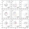Fig. 11. Same as in Fig. 10, but for matter flying away from the observer (ηmax = −45°) in the direction orthogonal to the rotation plane. Note different scales in panels.

Fig. 12. Stokes parameters of the infinitely compact spots and disk segments. Averaging was made over Δφ = 45° (i.e., a quarter of the circle). The upper and lower panels correspond to the absolute and relative Stokes parameters, respectively. Black, red, and green lines denote calculations of the infinitely small spot, while blue, violet, and yellow lines correspond to the parameters averaged over the segment. Note that several lines overlap in the lower panels.

If the extent of the hot spot becomes large, the PD drops, but it does not generally become zero. In the case of the disk ring, the net polarization arises owing to the broken symmetry as a result of the combined GR and SR effects. The net polarization of ∼5% was observed in Sgr A* (Event Horizon Telescope Collaboration 2024a). In Fig. 13, we show the net polarization (Stokes parameters) of the narrow disk ring at various radii, as a function of inclination. All points intersect at the origin, (q, u) = (0, 0), for i = 0 and the polarization generally increases with increasing i. The closer the disk ring is located to the BH, the higher the net polarization is, and the more the PA deviates from the direction along the disk normal. Hence, the u parameter of the net polarization can be used to obtain information about the proximity of matter to the compact object.

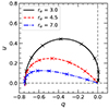Fig. 13. Relative Stokes parameters (in fractional units) of the disk ring (in the equatorial plane, η = 0, and rotating in the counterclockwise direction, σ = 90°) with vertical field B = Bz, as a function of inclination for different ring radii. Zero polarization corresponds to the case of i = 0 and increases, along the line, to i = 90°. Inclinations of i = 10°, 20°, and 30°...80° are marked with crosses. For inclinations of i > 90°, the curve is reflected around the u = 0 axis.

The polarimetric signatures of the disk ring depend on the inclination; hence, they are expected to change if the ring undergoes Lense-Thirring precession. The precessing disk rings scenario has been considered in the context of quasi-periodic eruptions (Raj & Nixon 2021; Arcodia et al. 2021). In the course of the Lense-Thirring precession, the inclination to the disk changes in a periodic way within limits set by the observer’s orientation relative to the BH spin and the misalignment angle between the BH spin and the plane of matter inflow. Intrinsic dependence of the polarimetric signatures on the inclination in Fig. 13 can then be converted to the observed profiles simply by computing the inclination of the disk at each precession phase (Veledina et al. 2013).

In Fig. 14, we show the dependence of the PD on the inclination angle in the case of the toroidal magnetic field, ϕ′ = 90°, and different radii. The case of r = 10⁴ might be relevant to the outer parts of the jet, as the ratio of the poloidal and toroidal components of the field decreases linearly with distance in the standard Blandford & Königl (1979) jet model. At small viewing angles, the PD is small because positive contributions to polarization coming from azimuthal angles φ and φ + 180° are (nearly) canceled by the negative contributions coming from the azimuthal angles φ ± 90°, for any φ. Light bending and aberration alter the PD at high inclinations, where otherwise (for slow motions and no light bending) the contributions from different parts of the disk have nearly the same PA; hence, the PD reaches a maximal value, P_s. For small distances from the compact object, we observe the effect of depolarization, caused by the different viewing angles of different parts of the disk; it is mostly pronounced at large inclinations. A good approximation for the case of a high radius is given by the sin^πi function (solid green line in Fig. 14).

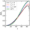Fig. 14. PD as a function of inclination, scaled to its maximal value, Ps, in the case of toroidal magnetic field (ϕ′ = 90°), equatorial counterclockwise rotation (η = 0, σ = 90°). The case re = 104 shows the dependence in the absence of relativistic effects and can be approximated well by sinπi.

For toroidal fields, the net polarization is aligned with the disk (or jet) axis for matter located at large distances. Close to the BH, the net PA deviates from this direction by up to 12°, achieved at r_e = 3. The PA deviation weakly depends on the inclination.

4.3. Image of the geometrically thick disk

Polarimetric images of two accreting supermassive BH environments recently obtained by the Event Horizon Telescope (Event Horizon Telescope Collaboration 2021, 2024a) show a consistent picture of spiral polarization pattern that is dominated by the azimuthally symmetric structure. The images correspond to the quiescent level of Sgr A* and M 87* emission and both show the rotationally symmetric pattern of PA rotation.

In Fig. 15, we plot the intensity (Eq. (35)) in the upper panel and the PD in the lower panel. The disk is assumed to be geometrically thick, with η = 30° at the ISCO, which translates into a constant height of h = 1.73R_S. We split the disk into 11 horizontal layers (one layer in the disk midplane and five layers below and above it) and assumed the elevation of matter above the midplane to be constant within each layer. We verified that this resolution is sufficient for convergence purposes. The observer inclination, i = 30°, and vertical magnetic field, B = B_z, were assumed. We obtained the characteristic image of an asymmetric ring-like structure, similar to the observed ones in M 87* and Sgr A*, as well as to the ones obtained in modeling of earlier works (Narayan et al. 2021; Vincent et al. 2024; Event Horizon Telescope Collaboration 2024b). However, the area of the region with high intensity is larger in the case of the thick disk, compared to the flat disk, and the shape of the BH shadow is squashed in the case of the thick disk. Both effects are caused by the presence of matter above the equatorial plane, at azimuthal angles close to zero (i.e., between the observer and the BH).

Fig. 15. Color-coded image of the thick accretion disk around a BH. In the upper panel, the color refers to the monochromatic intensity; in the lower panel, it refers to PD. The drop in PD close to the critical point can be seen in the upper left part of the image; otherwise, some depolarization is caused by the nonzero disk thickness.

The image of the disk is depolarized compared to the results for the narrow, flat ring. The depolarization is caused by the substantial vertical thickness: emission coming from different layers of the disk has different rotation angles of the polarization plane (see contours of PA rotation for different η in Fig. 2); hence, the net polarization is reduced. The dark area around coordinates ( − 4, 3) corresponds to the place where the disk is viewed face-on as a result of light-bending and aberration effects. For the vertical field, both intensity and PD decrease to zero here, and nonzero values appear as a result of the different position of this point for different disk layers. For the direct comparison to the data, additional beam depolarization and internal Faraday rotation (that is known to affect the polarization signatures in the submillimeter range, Event Horizon Telescope Collaboration 2021, 2024a; Wielgus et al. 2024) need to be considered. The latter effect can be taken into account by assuming that each layer between the emission point and the observer acts as a Faraday screen.

5. Summary

In this study, we have derived explicit analytical expressions for the transformation of polarization signatures for a fast-moving matter in the Schwarzschild metric in the case of the synchrotron emission. The rotation of the PA is caused by the joint effects of general and special relativity, as well as magnetic field orientation, which were considered separately. We considered different cases of moving matter direction, its elevation above and below the equatorial plane and magnetic field orientation, and computed the resulting PAs as a function of the azimuthal coordinate in the disk. We have further discussed potential applications of the developed formalism for the dynamic polarimetric signatures of spots orbiting around the compact object, as well as static images of geometrically thick accretion flows. We find that a number of the observed signatures can be explained by the nonzero thickness of the disk, which was generally omitted in previous analytical results. We highlight an important difference of the calculations presented in this work, compared to the polarization signatures in Minkowski space. The simple form of the derived expressions makes them attractive for the acceleration of the post-processing calculations, which can be done for a direct comparison with observations.

Acknowledgments

AV acknowledges support the Academy of Finland grant 355672. Nordita is supported in part by NordForsk. Authors thank V. Loktev, J. Poutanen and M. Wielgus for the useful discussions and comments on the paper.

References

Appendix A: Rotation of polarization angle

Light bending and relativistic aberration alter the direction of the photon path and hence change the direction of its electric field orientation, as seen by the observer. To determine the rotation of PA, we follow the method described in Loktev et al. (2022). For an arbitrary vector l, not collinear with the photon propagation direction $\widehat{\mathit{k}}$, we introduce the polarization basis, formed by two vectors orthogonal to each other and to the vector $\widehat{\mathit{k}}$ as

$$\begin{array}{c}\hfill \mathcal{B}(\widehat{\mathit{k}},\mathit{l})=\{{\widehat{\mathit{e}}}_1^{k,l},{\widehat{\mathit{e}}}_2^{k,l}\}=\{\frac{\mathit{l}-(\widehat{\mathit{k}}·\mathit{l})\widehat{\mathit{k}}}{|\widehat{\mathit{k}}\times \mathit{l}|},\frac{\widehat{\mathit{k}}\times \mathit{l}}{|\widehat{\mathit{k}}\times \mathit{l}|}\}.\end{array}$$(A.1)

The PA is given by the angle between the polarization plane of the photon and ${\widehat{\mathit{e}}}_1^{k,l}$, in the counterclockwise direction, as viewed by the observer intercepting the photon. For any other vector l₂, the new basis is $\mathcal{B}(\widehat{\mathit{k}},{\mathit{l}}_2)$, and the PA is given by the angle with respect to the new axis ${\widehat{\mathit{e}}}_1^{k,l_2}$. The new basis is built around the same photon direction, hence the PAs are different by the angle of rotation between the bases,

$$\begin{array}{c}\hfill \chi (\widehat{\mathit{k}},{\mathit{l}}_2\to \mathit{l})=\mathcal{B}({\widehat{\mathit{k}}}_0^{\prime },{\widehat{\mathit{B}}}^{\prime })\to \mathcal{B}({\widehat{\mathit{k}}}_0^{\prime },\widehat{\mathit{n}}),\end{array}$$(A.2)

that can be computed as

$$\begin{array}{c}\hfill tan\chi (\widehat{\mathit{k}},{\mathit{l}}_2\to \mathit{l})=\frac{\widehat{\mathit{k}}·(\mathit{l}\times {\mathit{l}}_2)}{\mathit{l}·{\mathit{l}}_2-(\widehat{\mathit{k}}·\mathit{l})(\widehat{\mathit{k}}·{\mathit{l}}_2)}.\end{array}$$(A.3)

For the synchrotron radiation of matter close to the BH, the photon is initially emitted along the direction ${\widehat{\mathit{k}}}_0\prime$ with polarization orthogonal to the magnetic field lines $\widehat{\mathit{B}}\prime$, the latter defines the basis $\mathcal{B}(\widehat{\mathit{k}}{\prime }_0,\widehat{\mathit{B}}\prime )$. Next, we shift to the description of the photon polarization plane orientation with respect to the normal to the plane of accreting matter $\widehat{\mathit{n}}$. Further, the relativistic aberration lead to the transition from $\widehat{\mathit{k}}{\prime }_0$ to ${\widehat{\mathit{k}}}_0$. Finally, the light bending changes the photon vector ${\widehat{\mathit{k}}}_0$ to $\widehat{\mathit{o}}$. Hence, we make the following steps between the bases:

$$\begin{array}{c}\hfill \mathcal{B}({\widehat{\mathit{k}}}_0^{\prime },{\widehat{\mathit{B}}}^{\prime })\to \mathcal{B}({\widehat{\mathit{k}}}_0^{\prime },\widehat{\mathit{n}})\to \mathcal{B}({\widehat{\mathit{k}}}_0,\widehat{\mathit{n}})\to \mathcal{B}(\widehat{\mathit{o}},\widehat{\mathit{n}}).\end{array}$$(A.4)

Each step is associated with the rotation of PA by the angle between the bases and is associated with different effects: magnetic field orientation χ^B, aberration χ^SR and light bending χ^GR. This can be explicitly written as

$$\begin{array}{c}\hfill \chi ={\chi }_0+{\chi }^{\mathrm{tot}}={\chi }_0+{\chi }^{\mathrm{B}}+{\chi }^{\mathrm{SR}}+{\chi }^{\mathrm{GR}},\end{array}$$(A.5)

where χ₀ = 90°.

Rotation associated with the magnetic field orientation is computed as the shift $\mathcal{B}(\widehat{{\mathit{k}}_{\mathbf{0}}\mathbf{\prime }},\widehat{\mathit{B}})\to \mathcal{B}(\widehat{{\mathit{k}}_{\mathbf{0}}\mathbf{\prime }},\widehat{\mathit{n}})$. Using Eq. A.3, χ^B is computed as

$$\begin{array}{c}\hfill {\chi }^{\mathrm{B}}=arctan\left(\frac{{\widehat{\mathit{k}}}_0^{\prime }·(\widehat{\mathit{n}}\times \widehat{{\mathit{B}}^{\mathbf{\prime }}})}{\widehat{\mathit{n}}·\widehat{{\mathit{B}}^{\mathbf{\prime }}}-({\widehat{\mathit{k}}}_0^{\prime }·\widehat{\mathit{n}})({\widehat{\mathit{k}}}_0^{\prime }·\widehat{{\mathit{B}}^{\mathbf{\prime }}})}\right).\end{array}$$(A.6)

Explicit analytical expression for the considered geometry and matter motions is given in Eq. (45).

The second and the third transformations have been described in Loktev et al. (2022) and we briefly mention them below for the sake of completeness. The transformation $\mathcal{B}(\widehat{\mathit{k}}{\prime }_0,\widehat{\mathit{n}})\to \mathcal{B}({\widehat{\mathit{k}}}_0,\widehat{\mathit{n}})$ is done via three steps:

$$\begin{array}{c}\hfill \mathcal{B}({\widehat{\mathit{k}}}_0^{\prime },\widehat{\mathit{n}})\to \mathcal{B}({\widehat{\mathit{k}}}_0^{\prime },\widehat{\mathit{v}})\to \mathcal{B}({\widehat{\mathit{k}}}_0,\widehat{\mathit{v}})\to \mathcal{B}({\widehat{\mathit{k}}}_0,\widehat{\mathit{n}}),\end{array}$$(A.7)

where the second step introduces zero rotation, as the vectors $\widehat{\mathit{k}}{\prime }_0$, $\widehat{\mathit{v}}$ and ${\widehat{\mathit{k}}}_0$ lie in the same plane. For the considered case $\widehat{\mathit{v}}\perp \widehat{\mathit{n}}$, the rotation angle is obtained as

$$\begin{array}{c}\hfill tan{\chi }^{\mathrm{SR}}=-\frac{\beta ({\widehat{\mathit{k}}}_0·(\widehat{\mathit{v}}\mathbf{\times }\widehat{\mathit{n}}))({\widehat{\mathit{k}}}_0·\widehat{\mathit{n}})}{1-{({\widehat{\mathit{k}}}_0·\widehat{\mathit{n}})}^2-\beta ({\widehat{\mathit{k}}}_0·\widehat{\mathit{v}})}.\end{array}$$(A.8)

The transformation $\mathcal{B}({\widehat{\mathit{k}}}_0,\widehat{\mathit{n}})\to \mathcal{B}(\widehat{\mathit{o}},\widehat{\mathit{n}})$ is done via an additional step involving the radial vector direction $\widehat{\mathit{r}}$:

$$\begin{array}{c}\hfill \mathcal{B}({\widehat{\mathit{k}}}_0,\widehat{\mathit{n}})\to \mathcal{B}({\widehat{\mathit{k}}}_0,\widehat{\mathit{r}})\to \mathcal{B}(\widehat{\mathit{o}},\widehat{\mathit{r}})\to \mathcal{B}(\widehat{\mathit{o}},\widehat{\mathit{n}}),\end{array}$$(A.9)

where, again, the second step introduces zero rotation, as the vectors ${\widehat{\mathit{k}}}_0$, $\widehat{\mathit{r}}$ and $\widehat{\mathit{o}}$ belong to the same plane in Schwarzschild metric (photon trajectories lie in plane). The resulting vector expression for the rotation angle is

$$\begin{array}{c}\hfill tan{\chi }^{\mathrm{GR}}=cos\eta \frac{(\widehat{\mathit{o}}·\widehat{\mathit{\phi }}){\tilde{g}}_1-({\widehat{\mathit{k}}}_0·\widehat{\mathit{\phi }}){\tilde{g}}_2}{{\tilde{g}}_1{\tilde{g}}_2+{cos}^2\eta (\widehat{\mathit{o}}·\widehat{\mathit{\phi }})({\widehat{\mathit{k}}}_0·\widehat{\mathit{\phi }})},\end{array}$$(A.10)

where

$$\begin{array}{cc}\hfill {\tilde{g}}_1& =(\widehat{\mathit{r}}·\widehat{\mathit{n}})-({\widehat{\mathit{k}}}_0·\widehat{\mathit{n}})({\widehat{\mathit{k}}}_0·\widehat{\mathit{r}}),\hfill \end{array}$$(A.11)

$$\begin{array}{cc}\hfill {\tilde{g}}_2& =(\widehat{\mathit{r}}·\widehat{\mathit{n}})-(\widehat{\mathit{o}}·\widehat{\mathit{n}})(\widehat{\mathit{o}}·\widehat{\mathit{r}}).\hfill \end{array}$$(A.12)

All Tables

All Figures

	Fig. 1. Geometry of the accreting matter around the BH. The fluid element is described by the radius vector, $\widehat{\mathit{r}}$, and velocity, $\widehat{\mathit{v}}$. Its trajectory is shifted from the midplane of the accretion disk by the angle, η. The observer is located in the direction of $\widehat{\mathit{o}}$, making an angle, i, with the disk normal, $\widehat{\mathit{n}}$.
In the text

Fig. 2. Contours of PA rotation (χSR + χGR) for different i = 30°, 60°, and 80° and η = 0, ±20° in the disk coordinates (r, φ), where r is measured in units of Schwarzschild radii. Azimuth increases in the counterclockwise direction, as is shown by the arrow in panel (a). Numbers on the contours correspond to the rotation angle (in degrees). The thick red line without a mark corresponds to ±90° rotation. Matter is assumed to have a purely circular Keplerian velocity in the counterclockwise direction (σ = 90°). The dashed line indicates the location of the ISCO. Contours corresponding to η = 0 (upper row) match those shown in Loktev et al. (2022). The effects of matter elevation above (or below) the orbital plane are clearly visible when comparing to the case of in-plane rotation. If matter is located in front of the BH (middle row), for the same radius from the BH the GR and SR effects appear to be less pronounced.

In the text

Fig. 3. Rotation of PA due to magnetic field orientation, as a function of azimuth (in disk coordinates) for different equatorial radii (measured in units of Schwarzschild radii): re = 3 (solid black), 5 (dashed red), 15 (dash-dotted green), and 50 (dotted blue). The matter is assumed to undergo circular, counterclockwise rotation (σ = 90°) with velocity following Luminet’s law. The upper panels correspond to a purely radial comoving magnetic field (ϕ′ = 90°) and the lower panels correspond to a purely toroidal field (ϕ′ = 0). The columns (left to right) correspond to the observer inclination, i = 30°, 60°, and 80°.

In the text

Fig. 4. Contours of constant total rotation angle (χtot) for the case of a toroidal magnetic field (σ = 90°, ϕ′ = 0) and the equatorial plane matter movement, in disk coordinates. We note the disappearance of the critical point, compared to the case of a vertical field, as the rotation is dominated by the changing magnetic field orientation (χB). The observed PA, χ, was obtained by adding χ0 = 90°.

In the text

Fig. 5. PA seen by the observer (χ) obtained for the angle η = 20°, for different radii, observer inclinations, and magnetic fields, as a function of the azimuth in the disk. The upper panels show the case of the radial field, the middle panels correspond to the purely toroidal field, and the lower panels correspond to the vertical field. The columns correspond, from left to right, to an increasing observer inclination: i = 30°, 60°, and 80°. The matter is assumed to rotate counterclockwise (σ = 90°), with a velocity following Luminet’s law.

In the text

Fig. 6. Difference between the PA obtained for the angle η = 20° and η = 0 (χtot(η = 20° ) − χtot(η = 0)), for different radii, observer inclinations, and magnetic fields, as a function of the azimuth in the disk coordinates. The upper panels show the case of the radial field, the middle panels correspond to the purely toroidal field, and the lower panels correspond to the vertical field. The columns, from left to right, correspond to an increasing observer inclination: i = 30°, 60°, and 80°. The matter is assumed to rotate counterclockwise (σ = 90), with a velocity following Luminet’s law.

In the text

Fig. 7. Effects of noncircular motion (σ) on the observed PA (χtot) for different inclinations (left to right: i = 30°, 60°, and 80°) and magnetic fields (upper panels: radial field, middle panels: toroidal field, lower panels: vertical field), as a function of the azimuth in the disk coordinates. Different directions of motion correspond to σ = 90° (solid black lines), 110° (dashed red), 150° (dash-dotted green), and 180° (dotted blue). The emitting matter is assumed to be located in the equatorial plane (η = 0) at a distance of r = 5, with a dimensionless velocity obeying Luminet’s law.

In the text

Fig. 8. Contours of constant GR and SR rotation angles (χGR + χSR), in disk coordinates. The position of the critical point is shown as a function of inclination for rotation caused solely by GR and SR effects (equivalent to B = Bz). The disk rotates counterclockwise (σ = 90°) in the equatorial plane, but at inclinations of i = 165° (a), 155° (b), and 140° (c) it is seen as rotating in the clockwise direction.

In the text

Fig. 9. Flux Stokes parameters, FQ and FU, obtained using η = 0, for different radii, B and i. Keplerian velocity and σ = 90° are assumed (note that for the considered inclinations, the observed matter movement is clockwise on the sky). Increasing saturation of color corresponds to progression of the spot along the azimuth. The time when the line intersects zero PD corresponds to the passage through the critical point. Note different scales in figures.

In the text

	Fig. 10. Stokes parameters, U and Q, for matter flying toward the observer (ηmax = 45°), in the direction orthogonal to rotation plane, at different launching azimuthal angles: φ0 = 90° (upper panels), 180° (middle panels), and 270° (lower panels). Note different scales in panels.
In the text

	Fig. 11. Same as in Fig. 10, but for matter flying away from the observer (ηmax = −45°) in the direction orthogonal to the rotation plane. Note different scales in panels.
In the text

Fig. 12. Stokes parameters of the infinitely compact spots and disk segments. Averaging was made over Δφ = 45° (i.e., a quarter of the circle). The upper and lower panels correspond to the absolute and relative Stokes parameters, respectively. Black, red, and green lines denote calculations of the infinitely small spot, while blue, violet, and yellow lines correspond to the parameters averaged over the segment. Note that several lines overlap in the lower panels.

In the text

Fig. 13. Relative Stokes parameters (in fractional units) of the disk ring (in the equatorial plane, η = 0, and rotating in the counterclockwise direction, σ = 90°) with vertical field B = Bz, as a function of inclination for different ring radii. Zero polarization corresponds to the case of i = 0 and increases, along the line, to i = 90°. Inclinations of i = 10°, 20°, and 30°...80° are marked with crosses. For inclinations of i > 90°, the curve is reflected around the u = 0 axis.

In the text

	Fig. 14. PD as a function of inclination, scaled to its maximal value, Ps, in the case of toroidal magnetic field (ϕ′ = 90°), equatorial counterclockwise rotation (η = 0, σ = 90°). The case re = 104 shows the dependence in the absence of relativistic effects and can be approximated well by sinπi.
In the text

	Fig. 15. Color-coded image of the thick accretion disk around a BH. In the upper panel, the color refers to the monochromatic intensity; in the lower panel, it refers to PD. The drop in PD close to the critical point can be seen in the upper left part of the image; otherwise, some depolarization is caused by the nonzero disk thickness.
In the text

References

- Aimar, N., Dmytriiev, A., Vincent, F. H., et al. 2023, A&A, 672, A62 [NASA ADS] [CrossRef] [EDP Sciences] [Google Scholar]
- Arcodia, R., Merloni, A., Nandra, K., et al. 2021, Nature, 592, 704 [NASA ADS] [CrossRef] [Google Scholar]
- Baganoff, F. K., Bautz, M. W., Brandt, W. N., et al. 2001, Nature, 413, 45 [Google Scholar]
- Beloborodov, A. M. 2002, ApJ, 566, L85 [Google Scholar]
- Blandford, R. D., & Königl, A. 1979, ApJ, 232, 34 [Google Scholar]
- Bogdanov, S., Lamb, F. K., Mahmoodifar, S., et al. 2019, ApJ, 887, L26 [NASA ADS] [CrossRef] [Google Scholar]
- Broderick, A. E., & Loeb, A. 2006, MNRAS, 367, 905 [Google Scholar]
- Chang, D. O., Johnson, M. D., Tiede, P., & Palumbo, D. C. M. 2024, ApJ, 974, 143 [NASA ADS] [CrossRef] [Google Scholar]
- Chen, K., & Shaham, J. 1989, ApJ, 339, 279 [NASA ADS] [CrossRef] [Google Scholar]
- Connors, P. A., & Stark, R. F. 1977, Nature, 269, 128 [Google Scholar]
- Connors, P. A., Piran, T., & Stark, R. F. 1980, ApJ, 235, 224 [Google Scholar]
- Dexter, J., & Agol, E. 2009, ApJ, 696, 1616 [Google Scholar]
- Do, T., Ghez, A. M., Morris, M. R., et al. 2009, ApJ, 691, 1021 [NASA ADS] [CrossRef] [Google Scholar]
- Do, T., Witzel, G., Gautam, A. K., et al. 2019, ApJ, 882, L27 [NASA ADS] [CrossRef] [Google Scholar]
- Dodds-Eden, K., Porquet, D., Trap, G., et al. 2009, ApJ, 698, 676 [NASA ADS] [CrossRef] [Google Scholar]
- Dovčiak, M., Muleri, F., Goosmann, R. W., Karas, V., & Matt, G. 2008, MNRAS, 391, 32 [CrossRef] [Google Scholar]
- Eckart, A., Baganoff, F. K., Schödel, R., et al. 2006a, A&A, 450, 535 [NASA ADS] [CrossRef] [EDP Sciences] [Google Scholar]
- Eckart, A., Schödel, R., Meyer, L., et al. 2006b, A&A, 455, 1 [NASA ADS] [CrossRef] [EDP Sciences] [Google Scholar]
- Event Horizon Telescope Collaboration (Akiyama, K., et al.) 2019, ApJ, 875, L1 [Google Scholar]
- Event Horizon Telescope Collaboration (Akiyama, K., et al.) 2021, ApJ, 910, L12 [Google Scholar]
- Event Horizon Telescope Collaboration (Akiyama, K., et al.) 2022, ApJ, 930, L12 [NASA ADS] [CrossRef] [Google Scholar]
- Event Horizon Telescope Collaboration (Akiyama, K., et al.) 2024a, ApJ, 964, L25 [NASA ADS] [CrossRef] [Google Scholar]
- Event Horizon Telescope Collaboration (Akiyama, K., et al.) 2024b, ApJ, 964, L26 [CrossRef] [Google Scholar]
- Gelles, Z., Himwich, E., Johnson, M. D., & Palumbo, D. C. M. 2021, Phys. Rev. D, 104, 044060 [NASA ADS] [CrossRef] [Google Scholar]
- Genzel, R., Schödel, R., Ott, T., et al. 2003, Nature, 425, 934 [NASA ADS] [CrossRef] [Google Scholar]
- Gillessen, S., Eisenhauer, F., Quataert, E., et al. 2006, ApJ, 640, L163 [NASA ADS] [CrossRef] [Google Scholar]
- Ginzburg, V. L., & Syrovatskii, S. I. 1965, ARA&A, 3, 297 [Google Scholar]
- GRAVITY Collaboration (Abuter, R., et al.) 2018, A&A, 618, L10 [NASA ADS] [CrossRef] [EDP Sciences] [Google Scholar]
- GRAVITY Collaboration (Abuter, R., et al.) 2020a, A&A, 638, A2 [NASA ADS] [CrossRef] [EDP Sciences] [Google Scholar]
- GRAVITY Collaboration (Jiménez-Rosales, A., et al.) 2020b, A&A, 643, A56 [CrossRef] [EDP Sciences] [Google Scholar]
- GRAVITY Collaboration (Abuter, R., et al.) 2023, A&A, 677, L10 [NASA ADS] [CrossRef] [EDP Sciences] [Google Scholar]
- Janssen, M., Falcke, H., Kadler, M., et al. 2021, Nat. Astron., 5, 1017 [NASA ADS] [CrossRef] [Google Scholar]
- Loktev, V., Salmi, T., Nättilä, J., & Poutanen, J. 2020, A&A, 643, A84 [NASA ADS] [CrossRef] [EDP Sciences] [Google Scholar]
- Loktev, V., Veledina, A., & Poutanen, J. 2022, A&A, 660, A25 [NASA ADS] [CrossRef] [EDP Sciences] [Google Scholar]
- Loktev, V., Veledina, A., Poutanen, J., Nättilä, J., & Suleimanov, V. F. 2024, A&A, 685, A84 [NASA ADS] [CrossRef] [EDP Sciences] [Google Scholar]
- Luminet, J. P. 1979, A&A, 75, 228 [Google Scholar]
- Matsumoto, T., Chan, C.-H., & Piran, T. 2020, MNRAS, 497, 2385 [NASA ADS] [CrossRef] [Google Scholar]
- Narayan, R., Palumbo, D. C. M., Johnson, M. D., et al. 2021, ApJ, 912, 35 [NASA ADS] [CrossRef] [Google Scholar]
- Nättilä, J., & Pihajoki, P. 2018, A&A, 615, A50 [NASA ADS] [CrossRef] [EDP Sciences] [Google Scholar]
- Pechenick, K. R., Ftaclas, C., & Cohen, J. M. 1983, ApJ, 274, 846 [Google Scholar]
- Pineault, S. 1977, MNRAS, 179, 691 [Google Scholar]
- Pineault, S., & Roeder, R. C. 1977, ApJ, 212, 541 [NASA ADS] [CrossRef] [Google Scholar]
- Ponti, G., George, E., Scaringi, S., et al. 2017, MNRAS, 468, 2447 [NASA ADS] [CrossRef] [Google Scholar]
- Poutanen, J. 2020, A&A, 640, A24 [NASA ADS] [CrossRef] [EDP Sciences] [Google Scholar]
- Poutanen, J., & Beloborodov, A. M. 2006, MNRAS, 373, 836 [NASA ADS] [CrossRef] [Google Scholar]
- Raj, A., & Nixon, C. J. 2021, ApJ, 909, 82 [NASA ADS] [CrossRef] [Google Scholar]
- Rybicki, G. B., & Lightman, A. P. 1979, Radiative Processes in Astrophysics (New York: Wiley-Interscience) [Google Scholar]
- Stark, R. F., & Connors, P. A. 1977, Nature, 266, 429 [NASA ADS] [CrossRef] [Google Scholar]
- Suleimanov, V. F., Poutanen, J., & Werner, K. 2020, A&A, 639, A33 [NASA ADS] [CrossRef] [EDP Sciences] [Google Scholar]
- Trippe, S., Paumard, T., Ott, T., et al. 2007, MNRAS, 375, 764 [NASA ADS] [CrossRef] [Google Scholar]
- Veledina, A., Poutanen, J., & Ingram, A. 2013, ApJ, 778, 165 [NASA ADS] [CrossRef] [Google Scholar]
- Vincent, F. H., Paumard, T., Perrin, G., et al. 2014, MNRAS, 441, 3477 [NASA ADS] [CrossRef] [Google Scholar]
- Vincent, F. H., Wielgus, M., Aimar, N., Paumard, T., & Perrin, G. 2024, A&A, 684, A194 [NASA ADS] [CrossRef] [EDP Sciences] [Google Scholar]
- Vos, J., Mościbrodzka, M. A., & Wielgus, M. 2022, A&A, 668, A185 [NASA ADS] [CrossRef] [EDP Sciences] [Google Scholar]
- Walker, M., & Penrose, R. 1970, Commun. Math. Phys., 18, 265 [NASA ADS] [CrossRef] [Google Scholar]
- Wielgus, M., Moscibrodzka, M., Vos, J., et al. 2022, A&A, 665, L6 [NASA ADS] [CrossRef] [EDP Sciences] [Google Scholar]
- Wielgus, M., Issaoun, S., Martí-Vidal, I., et al. 2024, A&A, 682, A97 [NASA ADS] [CrossRef] [EDP Sciences] [Google Scholar]
- Yfantis, A. I., Wielgus, M., & Mościbrodzka, M. 2024, A&A, 691, A327 [NASA ADS] [CrossRef] [EDP Sciences] [Google Scholar]
- Yusef-Zadeh, F., Roberts, D., Wardle, M., Heinke, C. O., & Bower, G. C. 2006, ApJ, 650, 189 [NASA ADS] [CrossRef] [Google Scholar]