| Issue |
A&A
Volume 676, August 2023
|
|
|---|---|---|
| Article Number | A79 | |
| Number of page(s) | 11 | |
| Section | Stellar atmospheres | |
| DOI | https://doi.org/10.1051/0004-6361/202346875 | |
| Published online | 09 August 2023 | |
M giants with IGRINS
II. Chemical evolution of fluorine at high metallicities
1
Lund Observatory, Division of Astrophysics, Department of Physics, Lund University,
Box 43,
221 00
Lund, Sweden
e-mail: This email address is being protected from spambots. You need JavaScript enabled to view it.
2
Department of Astronomy and McDonald Observatory, The University of Texas,
Austin, TX
78712, USA
Received:
11
May
2023
Accepted:
14
June
2023
Abstract
Context. The origin and evolution of fluorine in the Milky Way Galaxy is still under debate. In particular, the increase in the [F/Fe] in metal-rich stars found from near-IR HF lines is challenging to explain theoretically. Chemical evolution models with current knowledge of yields from different fluorine-producing stellar sources cannot reproduce these observations.
Aims. The aim of this work is to observationally study the Galactic chemical evolution of fluorine, especially for metal-rich stars. We want to investigate whether the significant rise in fluorine production at high metallicities can be corroborated. Furthermore, we want to explore the possible reasons for this upturn in [F/Fe].
Methods. We determined the fluorine abundances from 50 M giants (3300 < Teff < 3800 K) in the solar neighborhood spanning a broad range of metallicities (−0.9 < [Fe/H] < 0.25 dex). These stars are cool enough to have an array of lines from the HF molecule in the K band. We observed the stars with the Immersion GRating INfrared Spectrograph (IGRINS) spectrometer mounted on the Gemini South telescope and on the Harlan J. Smith Telescope at McDonald Observatory and investigate each of 10 HF molecular lines in detail.
Results. Based on a detailed line-by-line analysis of ten HF lines, we find that the R19, R18, and R16 lines (22 699.49, 22 714.59, and 22 778.25 Å) should primarily be used for an abundance analysis. The R15, R14, and R13 lines at 22 826.86, 22 886.73, and 22 957.94 Å can also be used, but the trends based on these lines show increasing dependence on the stellar parameters. The strongest HF lines, namely R12, R11, R9, and R7 lying at 23 040.57, 23 134.76, 23 358.33, and 23 629.99 Å should be avoided. The abundances derived from these strongest lines show significant trends with the stellar parameters, as well as a high sensitivity to variations in the stellar microturbulence, especially for coolest and most metal-rich stars. This leads to a huge scatter and high fluorine abundances for supersolar metallicity stars, not seen in the trends from the weaker lines for the same stars.
Conclusions. When estimating the final mean fluorine abundance trend as a function of metallicity, we neglect the fluorine abundances from the four strongest lines (R7, R9, R11, and R12) for all stars and use only those derived from R16, R18, and R19 for the coolest and most metal-rich stars. We confirm the flat trend of [F/Fe] found in other studies for stars in the metallicity range of −1.0 < [Fe/H] < 0.0 dex. We also find a slight enhancement at super-solar metallicities (0 < [Fe/H] < 0.15 dex) but we cannot confirm the upward trend seen at [Fe/H] > 0.25 dex. The HF line is intrinsically temperature sensitive, which calls for studies of stars with highly accurate and homogeneous stellar parameters. The spread in our trend is presumably caused by the temperature sensitivity. We need more observations of M giants at super-solar metallicities with a spectrometer that covers as many of the HF lines as possible, for instance the IGRINS spectrometer, to confirm whether the metal-rich fluorine abundance upturn is real or not.
Key words: stars: abundances / solar neighborhood / stars: late-type
© The Authors 2023
 Open Access article, published by EDP Sciences, under the terms of the Creative Commons Attribution License (https://creativecommons.org/licenses/by/4.0), which permits unrestricted use, distribution, and reproduction in any medium, provided the original work is properly cited.
This article is published in open access under the Subscribe to Open model. This email address is being protected from spambots. You need JavaScript enabled to view it. to support open access publication.
1 Introduction
The chemical evolution of the Milky Way Galaxy can be deciphered from the chemical nature of the stars belonging to the stellar populations that make up its components (e.g., the Galactic disk, bulge, halo). The study of chemical evolution is enabled by the fact that the photospheric abundances of individual elements derived from absorption lines in stellar spectra trace the chemistry of the gas in the interstellar medium from which the stars were formed. The chemical evolution trends of observed elemental abundance ratios for different stellar populations can also open up the possibility to explore the dominant production sites or progenitors of each element by comparison with trends from theoretical chemical evolution models.
While the elements such as O, Mg, Si, P, and Ti have been inferred to form in massive stars based on such investigations (Chieffi & Limongi 2004; Cescutti et al. 2012; Nomoto et al. 2013; Matteucci 2021), there are many elements whose origin and progenitors are still under debate. Fluorine is one such element. From theory, multiple production sites have been suggested, such as rapidly rotating massive stars (Prantzos et al. 2018), thermal pulses in asymptotic giant branch (AGB) stars (Forestini et al. 1992; Straniero et al. 2006), and the neutrino-process in core collapse supernovae (Woosley & Haxton 1988) and in novae (José & Hernanz 1998; Spitoni et al. 2018). Whether or not helium burning phases in Wolf-Rayet (WR) stars (Meynet & Arnould 2000; Palacios et al. 2005) contribute to the cosmic budget of fluorine is uncertain. From observations, multiple production sites have also been suggested (see, e.g., Ryde et al. 2020; Ryde 2020).
A theoretical difficulty is the large uncertainties in the 19F yields (in M⊙) from several of the above-mentioned production sites, such as WR and novae, as well as differences in the mass and metallicity ranges adopted in different stellar yield calculations. There is also no final consensus on the initial rotational velocities adopted for massive stars and their metallicity dependences. Thus, it is difficult to use chemical evolution models that adopt different stellar yields as their input parameter to pinpoint the exact production sites in different metallicity ranges. Many recent studies have explored the variation in the fluorine abundance trends resulting from chemical evolution models that adopt different combinations of the above-mentioned parameters and assuming different progenitors (Spitoni et al. 2018; Grisoni et al. 2020; Womack et al. 2023).
From an observational perspective as well, there are many challenges in the measurement of the fluorine abundances from stellar spectra. First, the cosmic abundance of fluorine is generally very low. It is three orders of magnitude lower than that of its immediate neighbors in the periodic table (C, N, O, Ne, Na, Mg, Al, and Si). This is a reflection of its unique formation channels, where Galactic fluorine is not synthesized in the main nuclear burning phases of stars (Clayton 2003). Although newly formed fluorine nuclei in stellar interiors readily react with hydrogen and helium, there are processes that can synthesize it in order for it to survive and contribute to the buildup of the cosmic reservoir of fluorine. Second, there are not many diagnos-tically useful spectra lines from which the fluorine abundances can be determined. There are no strong atomic fluorine lines at optical or infrared wavelengths, and there are only a few accessible molecular lines in the form of vibration-rotational lines from the HF molecules in the rather crowded, and telluric affected, infrared regimes.
The HF lines have been used to determine fluorine abundances in AGB stars (Jorissen et al. 1992; Abia et al. 2009, 2010, 2015, 2019); in giants in globular clusters (de Laverny & Recio-Blanco 2013a,b; Guerço et al. 2019b); in dwarfs (Recio-Blanco et al. 2012); in field G, K, and M giants in the Galactic disk (Jönsson et al. 2014b, 2017b; Pilachowski & Pace 2015; Guerço et al. 2019a; Ryde et al. 2020; Ryde 2020); in Galactic bulge stars (Jönsson et al. 2014a); and recently in the Galactic nuclear star cluster (Guerço et al. 2022). Among these studies, only a handful have determined the fluorine abundances for stars at super-solar metallicities (i.e., stars with [Fe/H]>0dex; see, e.g., Jönsson et al. 2017b; Ryde et al. 2020; Guerço et al. 2022). The general finding in these studies is an enhanced fluorine-to-iron abundance ratio, as well as a significant upturn with increasing metallicity, which is interpreted as a secondary behavior of fluorine (Ryde et al. 2020). Chemical evolution models have been unable to reproduce this trend for thin and thick disk stars (e.g., Spitoni et al. 2018). Suggested reasons for this include large uncertainties concerning the nucleosynthesis of fluorine (Spitoni et al. 2018); the need to invoke uncertain production sites like AGB stars contributing at later times, high mass-loss from metal-rich, massive stars, and/or novae (Grisoni et al. 2020); large uncertainties in the fluorine yields at super-solar metal-licities; and differences in the stellar composition compared to the local gas of the interstellar medium. The last is expected since at super-solar metallicities, stars are expected to have formed in the inner disk and migrated to the solar neighborhood (Womack et al. 2023). Thus, this upturn in fluorine at supersolar metallicities still remains a mystery, and is the subject of this paper.
The vibrational-rotational molecular line of HF at λair = 23 358.33 Å is most commonly used to determine fluorine abundance in the above-mentioned studies. This is primarily owing to the fact that the line is sufficiently strong, least affected (blended) by lines of other elements or molecules contained in the stellar atmosphere, and not affected by telluric lines. Other HF lines become considerably weaker for spectral types hotter than M type (Teff > 3900 k), which are the stellar types used in most previous studies. Another reason is that some instruments used to obtain K-band spectra do not record the full K band and will have gaps in wavelength. This might result in the absence of many of the other HF lines in the observed spectra. The first issue can be solved by targeting and obtaining the spectra of the cooler giants of M type (Teff < 3900 K), which will have stronger HF lines. An instrument such as the Immersion GRating INfrared Spectrograph (IGRINS; Yuk et al. 2010; Wang et al. 2010; Gully-Santiago et al. 2012; Moon et al. 2012; Park et al. 2014; Jeong et al. 2014) provides spectra spanning the full H and K bands (1.45–2.5 µm), which therefore will be able to record all possible R-branch lines of HF, all lying in the K band, solving the second issue.
In this paper we used IGRINS spectra of 50 cool giants in the solar neighborhood, stars of spectral type M spanning a broad range of metallicities (−0.9 < [Fe/H] < 0.25 dex). For these stars we determined the fluorine abundances from ten HF molecular lines. We carried out detailed line-by-line analysis and plotted individual fluorine abundance trends as a function of Teff, log ɡ, [Fe/H], and ξmicro to investigate whether a similar upturn in fluorine abundances at super-solar metallicities is evident for the cool M giants as well.
Our observations and data reduction procedure are described in Sect. 2. The determination of the fluorine abundance using the Spectroscopy Made Easy (SME) code is described in Sect. 3, followed by results and discussion in Sects. 4 and 5, respectively. Finally, we present our concluding remarks in Sect. 6.
2 Observations and data reduction
We thus determine the fluorine abundance for 50 M stars from high-resolution K-band spectra observed with the IGRINS spec-trograph. IGRINS provides a spectral resolving power of R ~ 45 000, and the reductions were done with the IGRINS PipeLine Package (IGRINS PLP; Lee et al. 2017) to optimally extract the telluric corrected, wavelength calibrated spectra after flat-field correction (Han et al. 2012; Oh et al. 2014). The spectra were then re-sampled and normalized in iraf (Tody 1993), but to take care of any residual modulations in the continuum levels, we focused on defining defining specific local continua around the HF line being studied. Finally, the spectra are shifted to laboratory wavelengths in air after a stellar radial velocity correction. The average signal-to-noise ratio (S/N) provided by the Raw & Reduced IGRINS Spectral Archive (RRISA; Sawczynec et al. 2022), is the average S/N for K band, and is per resolution element. It varies over the orders and it is lowest at the ends of the orders of the spectra of our stars range from 65 to 400, with most spectra having S/N> 100 (Nandakumar et al. 2023).
The 50 stars were also analyzed for their fundamental parameters in Nandakumar et al. (2023), where further details of the observations and data reduction are given. Apart from six stars from the IGRINS spectral library archive (Park et al. 2018; Sawczynec et al. 2022), which were observed at McDonald Observatory, the stars were observed at the Gemini South telescope (Mace et al. 2018) within the programs GS-2020B-Q-305 and GS-2021A-Q302 from January to April 2021.
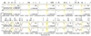 |
Fig. 1 Ten HF lines used to determine fluorine abundances. The top two rows show the observed spectra (black circles) for five HF lines (R19, R18, R16, R15, and R14) of one metal-rich star (32) and one metal-poor star (44); the stellar parameters (Teff, log ɡ, [Fe/H], and ξmicro) are to the left. The bottom two rows show the observed spectra for the remaining five HF lines (R13, R12, R11, R9, and R7) of the same two stars. The orange line denotes where the telluric lines lie before the telluric correction, and the red band the variation in the synthetic spectrum for ± 0.2 dex difference in fluorine abundance. The green line shows the synthetic spectrum without HF. The [F/Fe] values are also listed for each line. All identified atomic and molecular lines are denoted above the spectra. |
HF line data for the R branch (v″ = 0 to v′ = 1) lines used in this study.
3 Analysis
The fluorine abundances were derived from vibrational-rotational lines from the HF molecule. For a given star, defined by its stellar parameters, Teff, log ɡ, [Fe/H], and ξmicro (determined by Nandakumar et al. 2023), we synthesized model spectra using the Spectroscopy Made Easy code (SME; Valenti & Piskunov 1996, 2012). The synthesis uses one-dimensional (1D) Model Atmospheres in a Radiative and Convective Scheme (MARCS) stellar atmosphere models (Gustafsson et al. 2008), which are hydrostatic in spherical geometry, computed assuming LTE, chemical equilibrium, homogeneity, and conservation of the total flux. A relevant stellar atmosphere model is chosen by interpolating in a grid of MARCS models. The fluorine abundance is then set free and SME generates and fits multiple synthetic spectra with varying fluorine abundances. The final stellar abundance derived from the spectral line corresponds to the synthetic spectrum that best matches the observed spectrum by means of χ2 minimization method.
In Jönsson et al. (2014a), a comprehensive line list of the vibrational-rotational H19F lines (the R and P branches of the v″ = 0 to v′ = 1 band) in the K and L spectral bands are provided. The R branch lines lie toward the high-wavelength edge of the K band, with the R4-R91 lines being the strongest. The transition probabilities of the R7 to R19 lines do not vary much, but the series get increasingly weaker with increasing excitation energy of the lower rotational level (i.e., with increasing R-number). We were able to derive abundances from ten lines, namely the R7, R9, R11, R12, R13, R14, R15, R16, R18, and R19 lines. The other lines are heavily affected by blends or telluric lines and cannot be used to derive abundances.
The details of the ten HF absorption lines are listed in Table 1. For the surrounding atomic lines we used the modified line-list described in Nandakumar et al. (2023). The line data for the CO, CN, and OH molecular lines were adopted from the line lists of Li et al. (2015), Brooke et al. (2016), and Sneden et al. (2014), respectively.
3.1 Fundamental stellar parameters
Nandakumar et al. (2023) simultaneously determined Teff, log g, [Fe/H], ξmicro, [C/Fe], and [N/Fe] via an iterative spectroscopic method. In this method the effective temperature is mainly constrained by selected Teff-sensitive OH lines, the metallicity by selected Fe lines, the microturbulence by different sets of weak and strong lines, and the C and N abundances by selected CO and CN molecular lines. These abundances ensure that the CO and CN lines are fitted, which is especially important for the HF lines that are blended in part with CN and/or CO lines. The surface gravity is determined based on the effective temperature and metallicity by means of the Yonsei-Yale (YY) isochrones assuming old ages of 2-10 Gyr (Demarque et al. 2004), which is appropriate for low-mass giants. The final stellar parameters and C, N, O abundances determined for the 50 solar neighborhood stars are listed in Table 2.
Stellar parameters, [C/Fe], [N/Fe], [O/Fe], and mean [F/Fe] values along with the standard error of mean (from line-by-line abundances) for each star determined in this work.
3.2 Determination of F abundance
We determine the individual fluorine abundances from each of the ten HF lines for all studied stars. In Fig. 1 we show the synthetic spectra fit (crimson line) to the first five HF lines (R19, R18, R16, R15, and R14; top two rows) and the last five HF lines (R13, R12, R11, R9, and R7; bottom two rows) in the re-sampled observed spectra (black circles) of one metal-rich star 2M14333081-6221450 (32) and one metal-poor star 2M18522108-3022143 (44). We demonstrate the sensitivity of each HF line to the fluorine abundance with the red band that shows the variation in the synthetic spectra with Δ[F/Fe] = ±0.2 dex. We also indicate the star-specific telluric lines used for telluric correction in orange to highlight where they lie, and thus where some residuals might prevail, and to highlight where the noise is expected to be greater than in the rest of the spectrum. We note that the elimination of the telluric lines in general works very well. The yellow bands in each panel represent the line masks defined for the HF lines wherein SME fits the observed spectra by varying the fluorine abundance and finds the best synthetic spectra fit by chi-square minimization. The green line shows the synthetic spectrum without HF, thus indicating any possible known blends lying in the wavelength range of the HF line. We note that the line R11 has a dominant CO blend; the R7 and R12 lines have very strong CO lines to the left and right, respectively; and the R14, R15, R18, and R19 lines are blended by weak CN lines. The rest of the lines, namely, R16, R13, and R9, are the ones least affected by neighboring lines or molecules. The [F/Fe] values corresponding to the best fit case for each line is also listed in each panel.
We also carried out a detailed visual inspection of each HF line in every stellar spectrum to select only the lines of highest quality, those unaffected by noise, spurious features, and/or bad telluric corrections. Based on this, we found the HF lines at 23 134.76 Å (R11) and 23 358.33 Å (R9) (the third and fourth lines in the bottom panels in Fig. 1) to be of good quality for all 50 stars. The next−best quality lines are HF lines at 22 778.25 Å (R16) and 22 886.73 Å (R14) that are found to be of low quality only for around four to six stars. The HF line at 22 699.49 Å (first line in the top panels shown in the figure) is found to have the lowest quality, which makes it useful in only ~50% of the stars. The finally selected fluorine abundances, [F/Fe], determined from each HF line are listed in the Table 3.
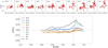 |
Fig. 2 Individual [F/Fe] vs. [Fe/H] trends. Top panels: [F/Fe] vs. [Fe/H] for the 50 solar neighborhood M giants (red circles) determined from the six K-band molecular HF lines (each panel) in the IGRINS spectra. All are scaled to the following solar abundances: A(F)⊙ = 4.43 (Lodders 2003) and A(Fe)⊙ = 7.45 (Grevesse et al. 2007). There is an evident increase and large scatter in [F/Fe] determined from the four reddest and strongest HF lines at 23 040.57 Å (R12), 23 134.76 Å (R11), 23 358 Å (R9), and 23 629.99 Å (R7) for stars with [Fe/H] ~ 0 dex and above (not evident in other lines) |
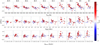 |
Fig. 3 [F/Fe] vs. Teff (top panels), log g (middle panels), and ξmicro (bottom panels). The color-coding indicates the respective metallicity (see color bar at right). The horizontal panels in each row are arranged in increasing order of wavelengths of the ten HF lines from which [F/Fe] was determined. |
[F/Fe] determined from the six HF lines after careful visual inspection of every star spectrum.
4 Results
In this section, we investigate the Galactic chemical evolution trend of fluorine in the solar neighborhood. To this end, we plot the [F/Fe] versus [Fe/H] for the fluorine abundances determined from individual HF lines in order to investigate if all of them show a similar upturn at super-solar metallicities to that seen in the case of warmer stars (see, e.g., Ryde et al. 2020; Ryde 2020). We further explore the nature of the individual fluorine abundance trends with respect to Teff, log g, [Fe/H], and ξmicro, as well as their sensitivity to a change in the microturbulence, ξmicro, which is indicative of the degree of saturation and how insensitive the line might be to the abundance. We also explore the temperature sensitivity of the HF lines in general. Our aim is to choose the best set of HF lines to determine fluorine abundances for M giants.
4.1 Individual [F/Fe] versus [Fe/H] trends
In the top panels of Fig. 2, we plot the [F/Fe] versus [Fe/H] trends for the 50 solar neighborhood M giants (red circles) determined from each of the ten HF lines. The trends are quite flat with some scatter for first four lines. The scatter then increases with increasing wavelength of the line used, especially for the four last lines. The scatter increases significantly for the metal-rich stars.
In the bottom panel we plot the running means of the fluorine abundances determined from each line with different colors to enable a qualitative comparison of the trends derived from the individual lines. We note that the running means plotted here have to be evaluated including the large spread, especially for the lines with the largest wavelengths. In this panel we also see the flat trends, especially for sub-solar metallicities. However, we also see a small fluorine enhancement at super-solar metallicities, an enhancement that increases for lines with increasing wavelengths. The lines with the highest wavelengths (the reddest ones) show the largest scatter and the largest super-solar increase. It is clear that the different HF lines show different derived fluorine abundances for the same stars at super-solar metallicity, especially from the four reddest lines at λair > 23 040.57 Å. An interesting question is then what causes these inconsistent abundances that are derived for the most metal-rich stars.
We note that the line at 23 134.76 Å is heavily blended with a CO(v = 2–0) line as shown in Fig. 1. Since other similarly weak CO lines close by are modeled well, we are confident that the fluorine abundance can be determined from this blended line. However, the blend makes it impossible to define a mask for the HF line, which is sensitive to fluorine alone.
4.2 Trends with stellar parameters
In Fig. 3, we plot the fluorine abundances determined from each HF line as a function of Teff (top panels), log ɡ (middle panels), and ξmicro (bottom panels), all color-coded according to the respective metallicities. From the figure we see that there is no significant Teff bias evident in our sample of 50 stars. An exception are the four coolest stars (Teff < 3400 K), which are all metal rich ([Fe/H] > 0.0 dex) and show higher fluorine abundances. This should be kept in mind since there are also metal-rich stars that are warmer and which, inconsistently, do not show these high abundance values. We also note that we do not have any cool (Teff < 3400 K) metal-poor stars in our sample.
The abundance trends as a function of Teff for the six bluest lines (R13, R14, R15, R16, R18, and R19), ignoring the four coolest stars, show only slight slopes. Since there is a range of metallicities represented at all temperatures, apart for Teff < 3400 K, this slight trend with Teff shows up as a scatter in the final [F/Fe] versus [Fe/H] trend.
For the four reddest HF lines at λair > 23 000 Å (R7, R9, R11, and R12), including the commonly used line at 23 358.33 Å (R9), however, we see significant downward trends as a function of Teff with higher abundances for cooler stars and lower abundances for hotter stars. For these lines the [F/Fe] ratio ranges from ∼ −0.5 to 0.5 dex for the metal-rich stars. This large spread is not seen for the other lines.
With respect to the surface gravity, log ɡ, there are no significant trends in the fluorine abundances for the ten lines. There is, however, significant scatter in the abundances from the four reddest lines at λair > 23 000 Å, presumably reflecting the large scatter in abundance trends with Teff mentioned above. A similar large scatter is also evident for these four lines in the plot versus ξmicro.
4.3 Sensitivity to ξmicro
In this section, we investigate the sensitivity of the ten HF lines to the variation in ξmicro. We varied ξmicro by ±0.2 dex, which can be considered quite a small amount for the microturbulence in general, and determined fluorine abundances from all ten HF lines for every star. The difference in the abundances corresponding to the ξmicro variation, color-coded according to Teff, is shown in Fig. 4.
We see in the figure that the two lines at λair < 22770 Å (R18 and R19) are insensitive to microturbulence, and are therefore good for deriving an abundance. For the sequential lines, the metal-rich stars start showing sensitivity to a change in microturbulence. As we go redward in the series, this sensitivity accelerates. There is also a clear signature that the abundances estimated for the cool (Teff < 3500 K) stars are affected the most.
The abundances from the HF lines at wavelengths larger than 22 885 Å (R7 to R14) are increasingly sensitive to ξmicro even for lower metallicities. For the four strong lines at λ > 23 000 Å, the abundance is extremely sensitive to microturbulence, leading to ~0.1–0.15 dex variations in [F/Fe] that increase from low to high metallicities. The strong correlation with ξmicro for abundances from these four HF lines is an indication that these lines are strong and saturated, especially for the cool metal-rich stars. These lines are therefore not useful for deriving an abundance, for M giants.
We note that lower sensitivities to ξmicro were demonstrated in earlier works by Jönsson et al. (2014a, 2017b), and Guerço et al. (2019a). The stars investigated in these works are warmer, however, which means that the lines are not saturated, and hence are considerably less ξmicro sensitive. We find, in fact, a similar trend in which our warmer stars and more metal-poor stars show the least ξmicro sensitivity (see Fig. 4).
4.4 Sensitivity to effective temperature
Since molecular lines in general are temperature sensitive, we also investigated the sensitivity of the ten HF lines to the variation in Teff. We varied the temperature within the given uncertainties from the method deriving the effective temperatures as given in Nandakumar et al. (2023; i.e., ±100 K). We then determined the fluorine abundances from all ten HF lines for every star. The difference in the abundances are shown in the Fig. 5. We see that the derived abundances indeed vary as much as ±0.15 dex for a change of ±100 K. This is the largest uncertainty source in our analysis, and is indicated in Fig. 6.
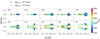 |
Fig. 4 Change in [F/Fe] as a function of variation in ξmicro. The color-coding indicates the Teff (see color bar at right) for the first five HF lines (R19, R18, R16, R15, and R14; top) and the last five HF lines (R13, R12, R11, R9, and R7; bottom). The variation in [F/Fe] for a +0.2 km s−1 change in ξmicro is shown by inverted triangles and for a −0.2 km s−1 change in ξmicro by circles. |
5 Discussion
In the previous section, we investigate the fluorine abundance trends from the ten HF lines as a function of stellar parameters and of their sensitivity to ξmicro. Based on this, we first attempt to choose the best HF lines to determine fluorine abundances for M giants followed by the comparison of our final [F/Fe] trend as a function of [Fe/H] to those available in the literature.
5.1 Best HF lines to determine fluorine abundances for M ɡiants
From the trends with metallicity of the ten HF lines it is obvious that the lines at 23 040.57, 23 134.76, 23 358.33, and 23 629.99 Å (i.e., the R7, R9, R11, and R12 lines) show a large scatter and do not follow the trends from the weaker lines. In addition, from the trends with the stellar parameters it is clear that the fluorine abundances derived from these four lines exhibit significant unexpected and inconsistent trends with Teff, log ɡ, and ξmicro, and show a large scatter in these plots. The R7, R9, R11, and R12 lines should therefore be avoided for abundance determinations in M giants (Teff < 3900 K). A reason for these trends and scatter might be that for cool, metal-rich, and low-gravity stars, these lines are strong, and could therefore be saturated (see, e.g., Gray 2008). This is actually reflected in the large spread in the microturbulence trends seen in Fig. 4. The abundances from these lines demonstrate strong correlations with ξmicro, especially for cool metal-rich stars.
We also find that the abundances from the three most blue-ward lines at 22 699.49, 22 714.59, and 22 778.25 Å (R19, R18, and R16) are the least susceptible to trends with Teff, log ɡ, and ξmicro. These lines should therefore primarily be used for abundance determinations for M giants. However, since they are increasingly weak, the slightly stronger lines at 22 826.86, 22 886.73, and 22 957.94 Å (R15, R14, and R13) could also be used, but with caution. The redder lines should always be avoided for M giants.
We also find that the strengths of the vibration-rotational lines of the HF molecule are very sensitive to uncertainties in the effective temperatures of the stars. This is not unexpected for molecules (OH is also very temperature sensitive; see, e.g., Nandakumar et al. 2023), which are sensitive to the temperatures in the line-forming regions. This could either be a result of uncertainties in the stellar parameters or in the detailed temperature structure itself of the model atmospheres. An intrinsic problem with the molecular lines of HF is that it is necessary to know the stellar temperatures with a high accuracy, which is difficult to achieve. Thus, the slight slopes in the abundance versus temperature plots might arise from a small systematic uncertainty in the Teff determination of the stars from Nandakumar et al. (2023).
We note that there is heavy CO(v = 2–0) blend in the line at 23 134.76 Å (R11; see Fig. 1). This blend can be taken care of provided that the similar CO lines close by in wavelength are modeled well. This ensures that the blend is properly modeled together with the HF line (which was successfully done for other elements in e.g. Nandakumar et al. 2022; Montelius et al. 2022).
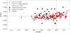 |
Fig. 6 Mean [Fe/Fe] vs. [Fe/H] for M giants in our sample (red circles) after excluding the fluorine abundances from the four reddest and strongest HF lines at 23 040.57 Å (R12), 23 134.76 Å (R11), 23 358 Å (R9), and 23 629.99 Å (R7). The black squares denote the stars in Pilachowski & Pace (2015), the blue circles the stars in Jönsson et al. (2014a), the plus signs the stars in Guerço et al. (2019a), and the gray diamonds and inverted triangles the stars in Ryde et al. (2020). |
5.2 [F/Fe] versus [Fe/H]: Comparison to literature
Due to the reasons elaborated in the previous section, we neglected the abundances from the four problematic lines (R7, R9, R11, and R12) for all stars in our sample while plotting the final [F/Fe] versus [Fe/H] trend. Furthemore, we only used the abundances from the three bluest HF lines (R16, R18, and R19) for cool and metal-rich stars (i.e., Teff < 3500 K and [Fe/H] > 0.0 dex). For all other stars, we plotted the mean [F/Fe] estimated from the six HF lines selected based on their quality (see Table 1). We show the final [F/Fe] versus [Fe/H] for the 50 stars in our sample in Fig. 6. As the comparison sample, we plot the fluorine abundances determined for stars in (Jönsson et al. 2014a, blue circles), Pilachowski & Pace (2015, black squares), Guerço et al. (2019a, gray plus signs), and Ryde et al. (2020, gray diamonds and inverted triangles).
Jönsson et al. (2014a) determined fluorine abundances from the R9 line using spectrum synthesis with SME for four bright nearby giants (including Arcturus) by analyzing their spectra observed with the Fourier Transform Spectrometer (FTS) mounted on the Kitt Peak National Observatory Mayall 4 m reflector. The Teff values were determined using angular diameter measurements taken from Mozurkewich et al. (2003), and the surface gravity, log ɡ, was based on the stellar radius, the parallax, and fits to evolutionary tracks. The metallicities were adopted from different spectroscopic archives and literature sources. All four stars have sub-solar metallicities, and apart from Arcturus with a Teff of 4226 K, the stars lie in the effective temperature range of 3700–3900 K.
Pilachowski & Pace (2015) determined the fluorine abundances also from the R9 line for nearly 80 G and K stars in the Galactic thin disk from spectra obtained with the Phoenix IR spectrometer on the 2.1 m telescope at Kitt Peak. They carried out the analysis using both spectral synthesis (with MOOG) and an equivalent width analysis (for weak lines). The stellar parameters for these stars have been adopted from various sources in the literature, with Teff in the range of 3800 K to 4800 K and metallicities in the range −0.6 < [Fe/H] < 0.3 dex. They estimated an average fluorine abundance of [F/Fe] = +0.23 ± 0.03 dex in the thin disk with a large scatter. In Fig. 6, we plot [F/Fe] for a subset of 52 stars, omitting the stars with upper limits.
Guerço et al. (2019a) estimated the fluorine abundances for a sample of Milky Way red giants from up to five HF lines (R16, R15, R14, R13, and R9) in K-band spectra obtained by observations using three infrared spectrographs: NOAO Phoenix (Hinkle et al. 2003), iSHELL spectrograph (Rayner et al. 2016), and the Fourier Transform Spectrometer (FTS) archive (Pilachowski et al. 2017). The Teff values, which were determined from photometric calibration, optical spectra, or adopted from APOGEE and from various other literature sources, range from 3400 K to 4900 K. The metallicities of the analyzed stars are limited to metal-poor to solar metallicities ([Fe/H] < 0.0 dex), as shown in Fig. 6.
Ryde et al. (2020) analyzed high-resolution K-band spectra of 61 Milky Way K giants obtained using the IGRINS and Phoenix spectrographs, and determined the fluorine abundances from the HF line at 23 358.33 Å (R9). They did not use other HF lines since the stars in their sample are warmer than the stars we analyzed here (4000-4600 K), resulting in weaker HF lines at shorter wavelengths. They also provided an upper limit of the fluorine abundances for several stars with very weak 23 358.33 Å lines (mostly hot, metal-poor, and high log g stars). A majority of the metal-rich stars in their study have the warmest Teff in their sample (Teff > 4300 K). Thus, for these stars the HF line is much weaker than for M giants in our sample, and therefore they cannot be expected to be saturated as is the case for cool M giants. Hence, the fluorine abundance determined from this line should be reliable. The stellar parameters in the Ryde et al. (2020) sample were determined from careful analysis from high-resolution optical spectra (Jönsson et al. 2017a). The stars in their sample cover a broader metallicity range of −1.2 < [Fe/H] < 0.4 dex.
The fluorine abundances determined for the four stars in Jönsson et al. (2014a) are consistent with our values in the same metallicity range. Our measurements are also consistent with the [F/Fe] values measured by Pilachowski & Pace (2015), although these show a larger scatter. Our final fluorine abundance trend agrees with the flat trend in Ryde et al. (2020) in the sub-solar metallicity range (i.e., for −1.0 < [Fe/H] < 0.0 dex). The scatter in the trend of Ryde et al. (2020) is larger (several stars with super-solar [F/Fe]), which is not the case with our trend. The sample from Guerço et al. (2019a) also exhibits a similarly flat trend for [Fe/H] > −0.4 dex, but decreases by ~0.1−0.2 dex for more metal-poor stars. This is a larger decrease than we see in that metallicity range. At super-solar metallicities there is a clear increase in [F/Fe] for stars from Ryde et al. (2020), while we find a slight enhancement ([F/Fe] ~ 0.1 dex) soon after solar metallicity. This could thus confirm a slight enhancement compared to more metal-poor stars. However, for stars more metal rich than [Fe/H] = 0.15 dex, we cannot confirm the steady and clear increase in [F/Fe] as seen in Ryde et al. (2020). The stars in our sample that have [Fe/H] > 0.2 dex are warmer than 3550 K and are therefore not affected that much by uncertainties in the microturbulence. Our derived fluorine abundances are therefore reliable. Our sample lacks stars with [Fe/H] higher than 0.25 dex to compare with similar stars in Ryde et al. (2020). All HF lines, however, are temperature sensitive and it has to be investigated whether the difference at [Fe/H] > 0.2 dex in these studies is due to uncertainties in the temperatures or whether it could be an unknown blend in the R9 line that mostly affects the warmer stars.
To conclude, we find a flat [F/Fe] versus [Fe/H] trend with no significant upturn at super-solar metallicities, but a hint of a slightly higher level of [F/Fe] for stars with [Fe/H] > 0 dex. The spread in our trend, which is smaller than that of Ryde et al. (2020), is presumably caused by the temperature sensitivity of the HF line. With the level of accuracy we have for the stellar parameters such a spread is indeed expected.
6 Conclusions
We carried out a detailed line-by-line abundance analysis of ten molecular HF lines in the IGRINS spectra of 50 Milky Way M giants (3300 K < Teff < 3800 K) in order to investigate the nature of the fluorine abundance trend as a function of metallicity. Of the 50 stars, 44 stars were observed within the programs GS-2020B-Q-305 and GS-2021A-Q302, while six were extracted from the IGRINS spectral library. The stellar parameters for these stars were determined based on the method using selected OH, CN, CO, and Fe lines in the H-band spectra described in Nandakumar et al. (2023).
Based on our investigations, we find that it is important to choose the lines wisely after detailed quality checks. We conclude that the R19, R18, and R16 lines (22 699.49, 22714.59, and 22 778.25 Å) of HF should primarily be used for abundance determinations for M giants, and can be used even for cool metal-rich stars. These are the least susceptible to trends with Teff, log ɡ, and ξmicro. However, since these lines are increasingly weak, the slightly stronger R15, R14, and R13 lines at 22 826.86, 22 886.73, and 22 957.94 Å could also be used, especially for lower metallicities. The strongest HF lines (R7, R9, R11, and R12) have significant trends with the stellar parameters, as well as a high sensitivity to variations in ξmicro, especially for the coolest and most metal-rich stars. These lines should therefore be avoided for abundance determinations in M giants (Teff < 3900 K).
Apart from the large trends of the derived abundances with the effective temperature of the stars for the four strongest HF lines, we also find a slight systematic trend with Teff for the six weaker lines. A reasonable explanation might be that this is caused by the high sensitivity of the molecular lines to the effective temperature and/or uncertainties in the temperature structure of the model atmosphere. These trends lead to an increased spread in the [F/Fe] versus [Fe/H] plots. This sensitivity is an intrinsic problem with lines from the HF molecule. One way to mitigate this problem would be to choose a sample of stars with a narrow range in Teff.
For cool (Teff < 3500 K) metal-rich stars, the HF lines (except R16, R18, and R19) show a higher sensitivity of the derived fluorine abundances to variations in ξmicro. This indicates that these lines might be strong or saturated, making their abundances uncertain. Thus, we neglected the fluorine abundances from the four strongest lines (R7, R9, R11, and R12) for all stars and used only those derived from R16, R18, and R19 for the coolest and most metal-rich stars when estimating the final mean fluorine abundance trend as a function metallicity.
From this trend we confirm the flat trend of Ryde et al. (2020) and Guerço et al. (2019a) for stars in the metallicity range of −1.0 < [Fe/H] < 0.0 dex and −0.6 < [Fe/H] < 0.0 dex. respectively. We also find a slight enhancement at super-solar metallicities (0 < [Fe/H] < 0.15 dex) that might be consistent with the general trend of Ryde et al. (2020). However, using our limited sample of stars at super-solar metallicities, we cannot confirm the upward trend seen at [Fe/H] > 0.15 dex in Ryde et al. (2020). We find lower fluorine abundances at these higher metallici-ties. Hence, we need more observations of many more M giants especially at high metallicities with their spectra from a capable high-resolution instrument like IGRINS to disentangle the correct nature of the fluorine trend.
Acknowledgements
We thank the anonymous referee for the constructive comments and suggestions that improved the quality of the paper. Henrik Jönsson is thanked for enlightening discussions. G.N. acknowledges the support from the Wenner-Gren Foundations and the Royal Physiographic Society in Lund through the Stiftelsen Walter Gyllenbergs fond. N.R. acknowledge support from the Royal Physiographic Society in Lund through the Stiftelsen Walter Gyllenbergs fond and Märta och Erik Holmbergs donation. This work used The Immersion Grating Infrared Spectrometer (IGRINS) that was developed under a collaboration between the University of Texas at Austin and the Korea Astronomy and Space Science Institute (KASI) with the financial support of the US National Science Foundation under grants AST-1229522, AST-1702267 and AST-1908892, McDonald Observatory of the University of Texas at Austin, the Korean GMT Project of KASI, the Mt. Cuba Astronomical Foundation and Gemini Observatory. This work is based on observations obtained at the international Gemini Observatory, a program of NSF’s NOIRLab, which is managed by the Association of Universities for Research in Astronomy (AURA) under a cooperative agreement with the National Science Foundation on behalf of the Gemini Observatory partnership: the National Science Foundation (United States), National Research Council (Canada), Agencia Nacional de Investigación y Desarrollo (Chile), Ministerio de Ciencia, Tecnología e Innovación (Argentina), Ministério da Ciência, Tecnologia, Inovações e Comunicações (Brazil), and Korea Astronomy and Space Science Institute (Republic of Korea). The following software and programming languages made this research possible: TOPCAT (version 4.6; Taylor 2005); Python (version 3.8) and its packages ASTROPY (version 5.0; Astropy Collaboration 2022), SCIPY (Virtanen et al. 2020), MATPLOTLIB (Hunter 2007) and NUMPY (van der Walt et al. 2011).
References
- Abia, C., Recio-Blanco, A., de Laverny, P., et al. 2009, ApJ, 694, 971 [NASA ADS] [CrossRef] [Google Scholar]
- Abia, C., Cunha, K., Cristallo, S., et al. 2010, ApJ, 715, L94 [NASA ADS] [CrossRef] [Google Scholar]
- Abia, C., Cunha, K., Cristallo, S., & de Laverny, P. 2015, A&A, 581, A88 [NASA ADS] [CrossRef] [EDP Sciences] [Google Scholar]
- Abia, C., Cristallo, S., Cunha, K., de Laverny, P., & Smith, V. V. 2019, A&A, 625, A40 [CrossRef] [EDP Sciences] [Google Scholar]
- Astropy Collaboration (Price-Whelan, A. M., et al.) 2022, ApJ, 935, 167 [NASA ADS] [CrossRef] [Google Scholar]
- Brooke, J. S. A., Bernath, P. F., Western, C. M., et al. 2016, J. Quant. Spec. Radiat. Transf., 168, 142 [NASA ADS] [CrossRef] [Google Scholar]
- Cescutti, G., Matteucci, F., Caffau, E., & François, P. 2012, A&A, 540, A33 [NASA ADS] [CrossRef] [EDP Sciences] [Google Scholar]
- Chieffi, A., & Limongi, M. 2004, ApJ, 608, 405 [NASA ADS] [CrossRef] [Google Scholar]
- Clayton, D. 2003, Handbook of Isotopes in the Cosmos (Cambridge University Press) [Google Scholar]
- de Laverny, P., & Recio-Blanco, A. 2013a, A&A, 555, A121 [NASA ADS] [CrossRef] [EDP Sciences] [Google Scholar]
- de Laverny, P., & Recio-Blanco, A. 2013b, A&A, 560, A74 [NASA ADS] [CrossRef] [EDP Sciences] [Google Scholar]
- Demarque, P., Woo, J.-H., Kim, Y.-C., & Yi, S. K. 2004, ApJS, 155, 667 [NASA ADS] [CrossRef] [Google Scholar]
- Forestini, M., Goriely, S., Jorissen, A., & Arnould, M. 1992, A&A, 261, 157 [NASA ADS] [Google Scholar]
- Gray, D. F. 2008, The Observation and Analysis of Stellar Photospheres (UK: Cambridge University Press) [Google Scholar]
- Grevesse, N., Asplund, M., & Sauval, A. J. 2007, Space Sci. Rev., 130, 105 [Google Scholar]
- Grisoni, V., Romano, D., Spitoni, E., et al. 2020, MNRAS, 498, 1252 [NASA ADS] [CrossRef] [Google Scholar]
- Guerço, R., Cunha, K., Smith, V. V., et al. 2019a, ApJ, 885, 139 [CrossRef] [Google Scholar]
- Guerço, R., Cunha, K., Smith, V. V., et al. 2019b, ApJ, 876, 43 [CrossRef] [Google Scholar]
- Guerço, R., Ramírez, S., Cunha, K., et al. 2022, ApJ, 929, 24 [CrossRef] [Google Scholar]
- Gully-Santiago, M., Wang, W., Deen, C., & Jaffe, D. 2012, SPIE Conf. Ser., 8450, 84502S [NASA ADS] [Google Scholar]
- Gustafsson, B., Edvardsson, B., Eriksson, K., et al. 2008, A&A, 486, 951 [NASA ADS] [CrossRef] [EDP Sciences] [Google Scholar]
- Han, J.-Y., Yuk, I.-S., Ko, K., et al. 2012, SPIE Conf. Ser., 8550, 85501B [NASA ADS] [Google Scholar]
- Hinkle, K. H., Blum, R. D., Joyce, R. R., et al. 2003, SPIE Conf. Ser., 4834, 353 [NASA ADS] [Google Scholar]
- Hunter, J. D. 2007, Comput. Sci. Eng., 9, 90 [NASA ADS] [CrossRef] [Google Scholar]
- Jeong, U., Chun, M.-Y., Oh, J. S., et al. 2014, SPIE Conf. Ser., 9154, 91541X [NASA ADS] [Google Scholar]
- Jönsson, H., Ryde, N., Harper, G. M., et al. 2014a, A&A, 564, A122 [NASA ADS] [CrossRef] [EDP Sciences] [Google Scholar]
- Jönsson, H., Ryde, N., Harper, G. M., Richter, M. J., & Hinkle, K. H. 2014b, ApJ, 789, L41 [CrossRef] [Google Scholar]
- Jönsson, H., Ryde, N., Nordlander, T., et al. 2017a, A&A, 598, A100 [NASA ADS] [CrossRef] [EDP Sciences] [Google Scholar]
- Jönsson, H., Ryde, N., Spitoni, E., et al. 2017b, ApJ, 835, 50 [CrossRef] [Google Scholar]
- Jorissen, A., Smith, V. V., & Lambert, D. L. 1992, A&A, 261, 164 [NASA ADS] [Google Scholar]
- José, J., & Hernanz, M. 1998, ApJ, 494, 680 [Google Scholar]
- Lee, J.-J., Gullikson, K., & Kaplan, K. 2017, https://doi.org/10.5281/zenodo.845059 [Google Scholar]
- Li, G., Gordon, I. E., Rothman, L. S., et al. 2015, ApJS, 216, 15 [NASA ADS] [CrossRef] [Google Scholar]
- Lodders, K. 2003, ApJ, 591, 1220 [Google Scholar]
- Mace, G., Sokal, K., Lee, J.-J., et al. 2018, SPIE Conf. Ser., 10702, 107020Q [NASA ADS] [Google Scholar]
- Matteucci, F. 2021, A&ARv, 29, 5 [NASA ADS] [CrossRef] [Google Scholar]
- Meynet, G., & Arnould, M. 2000, A&A, 355, 176 [NASA ADS] [Google Scholar]
- Montelius, M., Forsberg, R., Ryde, N., et al. 2022, A&A, 665, A135 [NASA ADS] [CrossRef] [EDP Sciences] [Google Scholar]
- Moon, B., Wang, W., Park, C., et al. 2012, SPIE Conf. Ser., 8450, 845048 [NASA ADS] [Google Scholar]
- Mozurkewich, D., Armstrong, J. T., Hindsley, R. B., et al. 2003, AJ, 126, 2502 [NASA ADS] [CrossRef] [Google Scholar]
- Nandakumar, G., Ryde, N., Montelius, M., et al. 2022, A&A, 668, A88 [NASA ADS] [CrossRef] [EDP Sciences] [Google Scholar]
- Nandakumar, G., Ryde, N., Casagrande, L., & Mace, G. 2023, A&A, 675, A23 [NASA ADS] [CrossRef] [EDP Sciences] [Google Scholar]
- Nomoto, K., Kobayashi, C., & Tominaga, N. 2013, ARA&A, 51, 457 [CrossRef] [Google Scholar]
- Oh, J. S., Park, C., Cha, S.-M., et al. 2014, SPIE Conf. Ser., 9147, 914739 [NASA ADS] [Google Scholar]
- Palacios, A., Arnould, M., & Meynet, G. 2005, A&A, 443, 243 [NASA ADS] [CrossRef] [EDP Sciences] [Google Scholar]
- Park, C., Jaffe, D. T., Yuk, I.-S., et al. 2014, SPIE Conf. Ser., 9147, 91471D [NASA ADS] [Google Scholar]
- Park, S., Lee, J.-E., Kang, W., et al. 2018, ApJS, 238, 29 [Google Scholar]
- Pilachowski, C. A., & Pace, C. 2015, AJ, 150, 66 [NASA ADS] [CrossRef] [Google Scholar]
- Pilachowski, C. A., Hinkle, K. H., Young, M. D., et al. 2017, PASP, 129, 024006 [CrossRef] [Google Scholar]
- Prantzos, N., Abia, C., Limongi, M., Chieffi, A., & Cristallo, S. 2018, MNRAS, 476, 3432 [Google Scholar]
- Rayner, J., Tokunaga, A., Jaffe, D., et al. 2016, SPIE Conf. Ser., 9908, 990884 [Google Scholar]
- Recio-Blanco, A., de Laverny, P., Worley, C., et al. 2012, A&A, 538, A117 [NASA ADS] [CrossRef] [EDP Sciences] [Google Scholar]
- Ryde, N. 2020, J. Astrophys. Astron., 41, 34 [NASA ADS] [CrossRef] [Google Scholar]
- Ryde, N., Jönsson, H., Mace, G., et al. 2020, ApJ, 893, 37 [CrossRef] [Google Scholar]
- Sawczynec, E., Mace, G., Gully-Santiago, M., & Jaffe, D. 2022, in AAS, 54, 203.06 [Google Scholar]
- Sneden, C., Lucatello, S., Ram, R. S., Brooke, J. S. A., & Bernath, P. 2014, ApJS, 214, 26 [Google Scholar]
- Spitoni, E., Matteucci, F., Jönsson, H., Ryde, N., & Romano, D. 2018, A&A, 612, A16 [NASA ADS] [CrossRef] [EDP Sciences] [Google Scholar]
- Straniero, O., Gallino, R., & Cristallo, S. 2006, Nucl. Phys. A, 777, 311 [NASA ADS] [CrossRef] [Google Scholar]
- Taylor, M. B. 2005, in ASP Conf. Ser., 347, 29 [Google Scholar]
- Tody, D. 1993, in ASP Conf. Ser., 52, 173 [NASA ADS] [Google Scholar]
- Valenti, J. A., & Piskunov, N. 1996, A&AS, 118, 595 [NASA ADS] [CrossRef] [EDP Sciences] [Google Scholar]
- Valenti, J. A., & Piskunov, N. 2012, Astrophysics Source Code Library [record ascl:1202.013] [Google Scholar]
- van der Walt, S., Colbert, S. C., & Varoquaux, G. 2011, Comput. Sci. Eng., 13, 22 [Google Scholar]
- Virtanen, P., Gommers, R., Oliphant, T. E., et al. 2020, Nat. Methods, 17, 261 [Google Scholar]
- Wang, W., Gully-Santiago, M., Deen, C., Mar, D. J., & Jaffe, D. T. 2010, SPIE Conf. Ser., 7739, 77394L [NASA ADS] [Google Scholar]
- Womack, K. A., Vincenzo, F., Gibson, B. K., et al. 2023, MNRAS, 518, 1543 [Google Scholar]
- Woosley, S. E., & Haxton, W. C. 1988, Nature, 334, 45 [NASA ADS] [CrossRef] [Google Scholar]
- Yuk, I.-S., Jaffe, D. T., Barnes, S., et al. 2010, SPIE Conf. Ser., 7735, 77351M [NASA ADS] [Google Scholar]
The R-number indicates the upper rotational level’s quantum number, J″
All Tables
Stellar parameters, [C/Fe], [N/Fe], [O/Fe], and mean [F/Fe] values along with the standard error of mean (from line-by-line abundances) for each star determined in this work.
[F/Fe] determined from the six HF lines after careful visual inspection of every star spectrum.
All Figures
|
Fig. 1 Ten HF lines used to determine fluorine abundances. The top two rows show the observed spectra (black circles) for five HF lines (R19, R18, R16, R15, and R14) of one metal-rich star (32) and one metal-poor star (44); the stellar parameters (Teff, log ɡ, [Fe/H], and ξmicro) are to the left. The bottom two rows show the observed spectra for the remaining five HF lines (R13, R12, R11, R9, and R7) of the same two stars. The orange line denotes where the telluric lines lie before the telluric correction, and the red band the variation in the synthetic spectrum for ± 0.2 dex difference in fluorine abundance. The green line shows the synthetic spectrum without HF. The [F/Fe] values are also listed for each line. All identified atomic and molecular lines are denoted above the spectra. |
| In the text | |
|
Fig. 2 Individual [F/Fe] vs. [Fe/H] trends. Top panels: [F/Fe] vs. [Fe/H] for the 50 solar neighborhood M giants (red circles) determined from the six K-band molecular HF lines (each panel) in the IGRINS spectra. All are scaled to the following solar abundances: A(F)⊙ = 4.43 (Lodders 2003) and A(Fe)⊙ = 7.45 (Grevesse et al. 2007). There is an evident increase and large scatter in [F/Fe] determined from the four reddest and strongest HF lines at 23 040.57 Å (R12), 23 134.76 Å (R11), 23 358 Å (R9), and 23 629.99 Å (R7) for stars with [Fe/H] ~ 0 dex and above (not evident in other lines) |
| In the text | |
|
Fig. 3 [F/Fe] vs. Teff (top panels), log g (middle panels), and ξmicro (bottom panels). The color-coding indicates the respective metallicity (see color bar at right). The horizontal panels in each row are arranged in increasing order of wavelengths of the ten HF lines from which [F/Fe] was determined. |
| In the text | |
|
Fig. 4 Change in [F/Fe] as a function of variation in ξmicro. The color-coding indicates the Teff (see color bar at right) for the first five HF lines (R19, R18, R16, R15, and R14; top) and the last five HF lines (R13, R12, R11, R9, and R7; bottom). The variation in [F/Fe] for a +0.2 km s−1 change in ξmicro is shown by inverted triangles and for a −0.2 km s−1 change in ξmicro by circles. |
| In the text | |
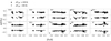 |
Fig. 5 Same as Fig. 4, but for variations in Teff. |
| In the text | |
|
Fig. 6 Mean [Fe/Fe] vs. [Fe/H] for M giants in our sample (red circles) after excluding the fluorine abundances from the four reddest and strongest HF lines at 23 040.57 Å (R12), 23 134.76 Å (R11), 23 358 Å (R9), and 23 629.99 Å (R7). The black squares denote the stars in Pilachowski & Pace (2015), the blue circles the stars in Jönsson et al. (2014a), the plus signs the stars in Guerço et al. (2019a), and the gray diamonds and inverted triangles the stars in Ryde et al. (2020). |
| In the text | |
Current usage metrics show cumulative count of Article Views (full-text article views including HTML views, PDF and ePub downloads, according to the available data) and Abstracts Views on Vision4Press platform.
Data correspond to usage on the plateform after 2015. The current usage metrics is available 48-96 hours after online publication and is updated daily on week days.
Initial download of the metrics may take a while.