| Issue |
A&A
Volume 675, July 2023
|
|
|---|---|---|
| Article Number | A165 | |
| Number of page(s) | 15 | |
| Section | Interstellar and circumstellar matter | |
| DOI | https://doi.org/10.1051/0004-6361/202346188 | |
| Published online | 18 July 2023 | |
Astrochemical models of interstellar ices: History matters
1
Laboratoire d’Astrophysique de Bordeaux (LAB), Univ. Bordeaux, CNRS, B18N, allée Geoffroy Saint-Hilaire,
33615
Pessac, France
e-mail: valentine.wakelam@u-bordeaux.fr
2
Université Bordeaux, CNRS,
LP2I Bordeaux, UMR 5797,
33170
Gradignan, France
3
Institut des Sciences Moléculaires (ISM), CNRS, Univ. Bordeaux,
351 cours de la Libération,
33400
Talence, France
4
Institut des sciences Moléculaires d’Orsay, CNRS, Université Paris-Saclay,
Bât 520, Rue André Rivière,
91405
Orsay, France
5
CY Cergy Paris Université, Observatoire de Paris, PSL Research University, Sorbonne Université, CNRS, LERMA,
95000
Cergy, France
6
Physique des Interactions Ioniques et Moléculaires, CNRS, Aix Marseille Univ.,
13397
Marseille, France
7
Laboratoire des deux infinis Irène Joliot Curie (IJClab), CNRS-IN2P3, Université Paris-Saclay,
91405
Orsay, France
Received:
20
February
2023
Accepted:
2
June
2023
Context. Ice is ubiquitous in the interstellar medium. As soon as it becomes slightly opaque in the visible, it can be seen for visual extinctions (AV) above ~1.5. The James Webb Space Telescope (JWST) will observe the ice composition toward hundreds of lines of sight, covering a broad range of physical conditions in these extinct regions.
Aims. We model the formation of the main constituents of interstellar ices, including H2O, CO2, CO, and CH3OH. We strive to understand what physical or chemical parameters influence the final composition of the ice and how they benchmark to what has already been observed, with the aim of applying these models to the preparation and analysis of JWST observations.
Methods. We used the Nautilus gas-grain model, which computes the gas and ice composition as a function of time for a set of physical conditions, starting from an initial gas phase composition. All important processes (gas-phase reactions, gas-grain interactions, and grain surface processes) are included and solved with the rate equation approximation.
Results. We first ran an astrochemical code for fixed conditions of temperature and density mapped in the cold core L429-C to benchmark the chemistry. One key parameter was revealed to be the dust temperature. When the dust temperature is higher than 12 K, CO2 will form efficiently at the expense of H2O, while at temperatures below 12 K, it will not form. Whatever hypothesis we assumed for the chemistry (within realistic conditions), the static simulations failed to reproduce the observed trends of interstellar ices in our target core. In a second step, we simulated the chemical evolution of parcels of gas undergoing different physical and chemical situations throughout the molecular cloud evolution and starting a few 107 yr prior to the core formation (dynamical simulations). We obtained a large sample of possible ice compositions. The ratio of the different ice components seems to be approximately constant for AV > 5, and in good agreement with the observations. Interestingly, we find that grain temperature and low AV conditions significantly affect the production of ice, especially for CO2, which shows the highest variability.
Conclusions. Our dynamical simulations satisfactorily reproduce the main trends already observed for interstellar ices. Moreover, we predict that the apparent constant ratio of CO2/H2O observed to date is probably not true for regions of low AV, and that the history of the evolution of clouds plays an essential role, even prior to their formation.
Key words: astrochemistry / ISM: clouds / ISM: molecules
© The Authors 2023
 Open Access article, published by EDP Sciences, under the terms of the Creative Commons Attribution License (https://creativecommons.org/licenses/by/4.0), which permits unrestricted use, distribution, and reproduction in any medium, provided the original work is properly cited.
This article is published in open access under the Subscribe to Open model. Subscribe to A&A to support open access publication.
1 Introduction
Interstellar grains are key ingredients for the formation of molecules in space, providing a catalytic surface. Molecular hydrogen, the most abundant molecule by far, is known to form exclusively on dust grains (see Wakelam et al. 2017a, for a review and references therein). With H2 having a low binding energy to the grain surface, only a very small fraction of the formed molecules stays on the grains and the vast majority returns into the gas-phase. However, this is not the case for other species. As the density increases in the cold and shielded environments of star forming regions, atoms and molecules formed in the gasphase (such as CO) are depleted from the gas and stick to the surface of the grains. Some reactions take place on these surfaces, leading to the formation of more or less complex species. Grain surfaces are very often cited as being of high importance because complex organic molecules are expected to form there (Herbst & van Dishoeck 2009). However, even before considering the formation of complex molecules, the chemistry of the main constituents of the ices (H2O, CO2, CO, and CH3OH) is still challenging for astrochemical models. Observations of interstellar ices in the infrared have shown that they are mostly composed of water. In addition, CO2 is also detected toward all lines of sight, with the exception of peculiar circumstellar environments such as around OH/IR stars, where pure water ice is observed (see Boogert et al. 2015, and references therein). Other molecules, such as CO, CH3OH, CH4, NH3, and H2CO have also been identified in various amounts (between a few percent to a few tens of percent with respect to H2O), depending on the observed environment. In cold cores, water ice is observed for visual extinction higher than a threshold AV of approximately 1.5 (i.e., half of the observed visual extinction threshold, considering only one side of the cloud), while CO ice is seen for AV higher than 3 and CH3OH for AV higher than 9. Finally, CO2 ice is observed with a threshold AV similar to H2O over all lines of sights.
In interstellar clouds, the formation of water ice is easily explained by chemical models as the hydrogenation of atomic oxygen is fast (no activation barrier) and requires only the diffusion of atomic hydrogen (very mobile) on the grain surfaces at very low temperatures (T ~ 10 K). The formation processes of NH3 and CH4 are similar to those H2O (easily formed on the surfaces) but chemical models form fewer of these species because the sticking of atomic N and C is in competition with their fast reactivity in the gas-phase to form CO and N2 (Daranlot et al. 2012). Specifically, CO is formed in the gas-phase and sticks to the surfaces. Although the formation of methanol from CO ices is challenging because of activation barriers for some of the hydrogenation steps and the existence of some dehydrogenation channels, chemical models can form large amounts of methanol ice (Garrod et al. 2007) even without the inclusion of photochemical or radiolysis formation pathways. Since its formation is not efficient at low temperatures, CO2 remains the most problematic icy molecule (Ruffle & Herbst 2001; Garrod & Pauly 2011; Vasyunin et al. 2017).
While current constraints on chemical models are based on a relatively small number of observations, data from the James Webb Space Telescope (JWST) will almost certainly call into question our current understanding. The majority of ice observations to date have been performed along single, pre-identified lines of sight. As such, our current picture of ice composition and evolution is limited to a reliance on deriving trends by comparing this small number of lines of sight (Boogert et al. 2015). Where multiple lines of sight in a single object have been surveyed (Murakawa et al. 2000; Pontoppidan et al. 2004; Boogert et al. 2011; Noble et al. 2013; Goto et al. 2018) – and, more specifically, where the lines of sight have not been selected in advance (i.e., when using slitless spectroscopy), local deviations from global trends in ice composition have been observed, at scales down to a few hundred au (Noble et al. 2017). In addition to the much higher sensitivity of this telescope as compared to previous satellites or ground based observations, JWST will observe the ice composition toward hundreds of line of sight, covering a large range of physical conditions of the interstellar medium, as proposed, for instance, by the IceAge project (McClure et al. 2017). The first results of ice observations with JWST toward three lines of sight using the MIRI (Yang et al. 2022) or a combination of MIRI, NIRSpec, and NIRCam (McClure et al. 2023) instruments have already demonstrated their capacity to provide high spectral resolution, high-sensitivity spectra of ices in molecular clouds when observing lines toward embedded protostars and highly extincted background stars, respectively.
In this work, we conduct a theoretical study of the chemical ice composition in a large range of cold core physical conditions in order to understand the formation of the main ice constituents and also make predictions for the sensitivity of the ice composition to the physical conditions, by considering those along the most diffuse lines of sight as well as those in the cold core. We start from an initial composition – gas-phase and mostly atomic – and compute time-dependent chemistry for a set of physical parameters. In doing so, we show that more sophisticated time-dependent physical conditions that follow the formation of cold cores from the earliest stages are needed to explain the general features of observed ice. The chemical model used for the simulations is described in Sect. 2. The static chemical simulations together with their results are given in Sect. 3. Section 4 presents the results of the dynamical simulations. The results of both sets of simulations are first compared in Sect. 5. In Sects. 6 and 7, we discuss the chemical processes involved in the chemistry of CO2 ices and the influence of the dust temperature. Section 8 presents our predictions on the ice composition as a function of visual extinction. In Sect. 9, we discuss the time-dependent formation of ice. We present our conclusions in the final section.
2 Chemical model
To make predictions on the ice composition, we used the three-phase gas-grain model, Nautilus. This numerical model computes the gas and ice composition as a function of time for a set of physical conditions (e.g., gas and dust temperature, visual extinction, density, and cosmic-ray ionization rate) starting from an initial gas phase composition. The model is flexible enough to be able to use either static physical conditions, set at the beginning of the calculation, or time-dependent ones. All important processes (gas-phase reactions, gas–grain interactions, grain surface processes) are included and solved with the rate equation approximation. Gas-phase reactions are described in Wakelam et al. (2015). Species from the gas-phase can physisorb at the surface of dust grains with an energy that depends on the binding energy of surface species (determined for water ice surfaces). They can desorb because of the dust temperature (Hasegawa et al. 1992), whole grain heating induced by cosmic-rays (following Hasegawa & Herbst 1993), impact of UV photons (photodesorption, Ruaud et al. 2016), exothermicity of surface reactions (chemical desorption, Minissale et al. 2016b), and sputtering by cosmic-rays (following Wakelam et al. 2021). Detailed descriptions of the non-thermal desorption processes included in Nautilus can be found in Wakelam et al. (2021). The Nautilus model is used in its three-phase version, which means that the molecules at the surface of the grains are divided into two separate phases. The first phase is composed of the first few monolayers of species on top of the grains (four in our case; see below for a more detailed explanation), while the rest of the molecules below these surface layers represents the bulk of the ice. The refractory parts of the grains (below the bulk) is chemically inactive. Both the surface and the bulk are chemically active. Photodissociation by direct UV photons and secondary photons induced by cosmic-rays are efficient in both phases. The diffusion (and thus reactivity) of the surface is higher than in the bulk while the species on the surface can desorb into the gas phase, contrary to the species in the bulk. Only sputtering by cosmic-rays can directly desorb species from the bulk ice. The relevant equations and chemical processes are described in Ruaud et al. (2016), and Wakelam et al. (2015, 2021).
With respect to the version used in Wakelam et al. (2021), three modifications to the code have been made. First, we implemented an automatic switch for the chemical desorption, depending on the water grain surface coverage. Since we are using the formalism of Minissale et al. (2016b) for the chemical desorption, two prescriptions are proposed by the authors: one for bare grains and one for grains covered by water, with the first shown to be more efficient than the second. We then switch from the first prescription to the second one if the grains are covered by more than four monolayers of molecules. The choice of these few layers corresponds to the following experimental observations. On the one hand, in the measurable case of the O+O reaction, it has been shown that the effect of an N2 preadsorbed layer makes the chemical desorption disappear once two monolayers are adsorbed (Minissale & Dulieu 2014). On the other hand, the thickness of the active chemical layer is also from one (Congiu et al. 2020) to a few monolayers in the case of water (Ioppolo et al. 2010). Four monolayers therefore seems to be a good compromise between these various situations. The second modification of the code is the implementation of a new module to compute the grain temperature using the approximation of Hocuk et al. (2017), which is a function of visual extinction and local UV field. Last, for the cosmic-ray ionisation rate (ζ), we used a prescription that depends on the visual extinction to take into account the attenuation with density. This prescription was determined by fitting the Fig. 6 of Neufeld & Wolfire (2017), which represents measurements of ζ through observed column densities of H2 and  . This fit gives the following formula:
 (1)
(1)
For AV smaller than 0.5, we assume a constant attenuated rate of ζ(0.5) (about 4 × 10⁻¹⁶ s−1). This formula is slightly different from the one used in Wakelam et al. (2021) to be more conservative at high visual extinction and closer to the model predictions of Padovani et al. (2022). Using the formula given in Wakelam et al. (2021), ζ would be 1.8 × 10⁻¹⁷ s−1 while it is 5 × 10⁻¹⁷ s−1 with the new formula. For all the simulations, we start from an initial chemical composition as listed in Table 1 (in which all elements are atoms, except hydrogen, which is entirely molecular).
Initial abundances (with respect to the total proton density).
3 Static simulations for L429-C
We run a first set of simulations using the physical conditions as observed in the cold core L429-C with no evolution of the physical conditions during the calculation of the chemistry.
3.1 Presentation of the L429-C cold core region
L429-C is a quiescent cold core located in the Aquila Rift (~200 pc, Stutz et al. 2009). There is no IR heating source inside. Herschel observations at 353 GHz from Sadavoy et al. (2018) provided dust temperature and opacity maps of the region. Based on the opacity map, Taillard et al. (2023) derived a H2 column density and subsequently, using a methodology from Bron et al. (2018), a volume H2 density. We refer the reader to Taillard et al. (2023) for details on the calculation and methods used. Figure A.1 in the appendix A shows the H2 column density (cm−2), the H2 volume density (cm−3), the visual extinction, and the dust temperature maps of the region. The maps are 200″ × 200″ size and contain 26 × 26 pixels1. The dust temperature as measured by Herschel ranges from 12 K to 18 K, while the H2 density goes from 5 × 103 cm−3 to 3 × 106 cm−3 and the visual extinction from 5 to more than 75. In this region, Boogert et al. (2011) estimated the column densities of H2O, CO2, and CH3OH ices toward four background stars using Spitzer observations (see their Table 6).
3.2 Model results
3.2.1 Using the observed dust temperature
For our first grid of chemical models, we have run Nautilus for each pixel of the maps shown in Fig. A.1, using the observed local physical conditions: proton density, visual extinction, and temperature. In the absence of good estimates of the gas temperature, based for instance on the excitation conditions of molecules, we have set the gas temperature equal to the dust temperature measured by Herschel (see also Taillard et al. 2023). This represents a fair approximation at moderate to high AV. To compute the molecular column densities from the model abundances, we multiplied the modeled abundances by the observed H2 column density at each position of the region, assuming that all the hydrogen was in the form of H2. The surface and bulk abundances from our models are summed to obtain the total column densities of icy molecules. The model results, column density as a function of visual extinction, are shown in Fig. 1 for two different times (105 yr and 106 yr), that we can consider as “early” and “late” times for the main ice constituents observed in cold cores (H2O, CO2, CO, and CH3OH). Superimposed on the figure, diamonds indicate the observed column densities of the molecules by Boogert et al. (2011). We note that CO ices were not targeted in the observational study and there is only one point of measurement for CO2. Whatever the time, whenever the AV is higher than about 10, using this static modeling approach, the CO2 ices are much more abundant than H2O – which is not not in line with what has been observed (see also Boogert et al. 2015).
In these simulations, as in most astrochemical simulations of cold cores, we start from atoms. This means that, as a function of time, there is a competition between the sticking of the gas-phase oxygen atoms onto the grains – that will be hydrogenated to form water – and their reactivity in the gas-phase to form CO. Once formed, CO will itself stick to the grains and can produce CO2 if some atomic oxygen is still available, and either CO or O can diffuse. One key ingredient in these processes is the dust temperature. In these simulations, the dust temperature is that observed by Herschel and shown in Fig. 2 as a function of visual extinction (see also Fig. A.1). The values range from 12 to 18 K. For temperatures above 12 K, the amount of hydrogen on the surface is rather low, preventing the efficient hydrogenation of oxygen and favoring the formation of CO2. The problem is of course not that simple because when looking at the early time in Fig. 1, we can see that at AV lower than 10, when the dust temperature is higher than 16 K, water is on the same order as CO2. At these low Av, with higher UV irradiation and lower density, the formation of CO is slower than the sticking of atomic oxygen onto the grains. As a consequence, water formation can occur but, as time goes on, CO in the gas-phase is formed and CO2 formation on the surface becomes more efficient, overtaking the water abundance.
It might be worth mentioning here that the representation of the results as column density as a function of visual extinction might be misleading. The increasing column density of H2O and CO2 with AV is an effect of an increase of H2 column density and not an increase of abundance of the species. In fact, the abundance of water and CO2 reaches a maximum at an AV of 10 (at 106 yr) of ~4 × 10⁻⁵ (with respect to H) for H2O and ~8 × 10⁻⁴ for CO2.
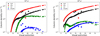 |
Fig. 1 Column density of the main ice constituents computed with Nautilus for the static physical conditions as observed in L429-C as a function of visual extinction (derived from Herschel observations). Diamonds represent the observed column densities by Boogert et al. (2011) on specific positions of the cloud. The model result at two different times are shown: 105 yr on the left and 106 yr on the right. The dust temperature is equal to that observed by Herschel. |
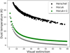 |
Fig. 2 Dust temperature as a function of visual extinction used for the models. In black: dust temperature measured by Herschel. In gray: dust temperature computed with Hocuk et al. (2017) approximation. In green: dust temperature computed with Hocuk et al. (2017) approximation plus 1 K (“Hocuk+1”). |
3.2.2 Computing the dust temperature
To test the impact of the adopted dust temperature on the ice composition, we ran the same set of models but computed the dust temperature using the prescription of Hocuk et al. (2017), which is a function of visual extinction and local UV field. The temperature obtained with this prescription is compared to the measured one in Fig. 2. In the same figure, we show the dust temperature if one Kelvin is added to this prescription (called “Hocuk+1” in the rest of the paper, see discussion in Sect. 7). Hocuk’s prescription is proportional to the Draine UV field strength (Draine 1978) to the power 1/5.9. In this work, we have used a value of one for this parameter in the absence of additional constraint. Our case Hocuk+1 can be obtained for 2 Draine UV field strength. For higher values, the dust temperature would also be shifted toward higher values. The predicted dust temperature also depends on the grains compositions. Hocuk’s relation was obtained by assuming carbonaceous-silicate mixtures. At a high visual extinction (approximately larger than 10), grain growth or icy mantles introduce larger uncertainties in the computed dust temperature (Hocuk et al. 2017). For the entire range of visual extinctions considered here, the dust temperature always remains below 11 K using Hocuk’s formula. For the gas temperature, in the absence of better estimates, we still used the temperature measured by Herschel. We note that within this range of values, the ice abundances will not be sensitive to this latter approximation.
Figure 3 shows the results of this model at two different times. In this case, because of the low temperature, CO2 is never efficiently produced. Water becomes the main ice constituent after 105 yr while CO is transformed into CH3OH with time. Again, with this modeling, we reproduce the observed general trends neither in L429-C nor in the other observed regions as summarized by Boogert et al. (2015). While the abundances of water and (at late times) methanol seem overall to be well reproduced, the CO2 abundance is highly underestimated and the CO abundance overestimated. The dust temperature seems to be a key ingredient in reproducing the observed ice composition at different visual extinctions.
The choice of the initial chemical composition affects some of the results. First, the amount of hydrogen already converted into H2 at the beginning of the simulations is an unknown, although observations show that the abundance of atomic hydrogen in dense regions should not be above a few 10−3. Starting the static simulations with this initial abundance of atomic hydrogen does not change the model results (see also Wakelam et al. 2021, for discussions). The CO molecule can also potentially form very early during the formation of the cold core (Bergin et al. 2004). Starting with some CO already formed can change the ice composition, as CO would have already started sticking earlier on the grains. We redid our static simulations starting with half of the carbon in the form of CO (decreasing in the appropriate amount the initial atomic oxygen abundance). At 105 yr, the CO ice column density is unchanged, but the water ice column density is slightly less at AV larger than 10 (similar to CO). The methanol column density is the most impacted as it is already at the same level than at 106 yr. At 106 yr, both simulations (starting from some molecular CO or only atoms) give similar results.
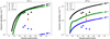 |
Fig. 3 Same as Fig. 1 but for the models in which the dust temperature is computed with the Hocuk et al. (2017) approximation (rather than the temperature derived from Herschel observations). |
3.3 Comparison with previous model
Using a different three-phase gas-grain model, Garrod & Pauly (2011) also studied the formation of ices. With their model, they were able to produce larger quantities of CO2 ices than we managed to do at 10 K. There are a number of differences between our model and theirs that can explain this difference. First, in their model, they form CO2 through the surface reaction COice + OHice → CO2ice + Hice. However, this reaction has a moderate activation barrier (which they assumed to be 80 K based on Ruffle & Herbst 2001), they also added a direct formation of CO2 – when an OH molecule is formed on top of a CO molecule on the surface. This mechanism can be seen as a two-step process. First, the formation of a van der Waals complex O…COice is more likely via a direct landing of an oxygen atom on top of an already physisorbed CO molecule. The hydrogenation of this complex is without barrier and leads to the formation of CO2 ice. We discuss this process further in Sect. 6. Garrod & Pauly (2011) are likely to have used different diffusion rates of molecules on the surface. Even though lower diffusion results in a higher probability of reaction for reactions with activation barriers, it reduces the efficiency of encounter on a surface. These authors have lower binding energies for atomic oxygen (800 K for them and 1660 K for us He et al. 2015), OH (2850 K for them and 4600 K for us, Wakelam et al. 2017b), CO (1150 K for them and 1300 K for us, Wakelam et al. 2017b), and HCO (1600 K for them and 2400 K for us, Wakelam et al. 2017b). For the binding energy of atomic oxygen, the experiments carried out by Ward et al. (2012) and Minissale et al. (2016a) also found high values. We note that the values used in our simulations are in good agreement with the recent review by Minissale et al. (2022). For the ratio of the diffusion energy versus binding energy, we use 0.4 for the surface layer (which is four monolayers), while Garrod & Pauly (2011) used a ratio that depends on the coverage of H2. In our case, we do not have depletion of H2 onto the grains because we include the encounter-desorption reaction from Hincelin et al. (2015). In our simulations, the key factor is the diffusion of atomic oxygen. As also pointed out by Garrod & Pauly (2011), the new numerical treatment of the competition between diffusion and reaction for chemical reactions with activation barriers (Chang et al. 2007; Garrod & Pauly 2011) strongly diminishes the effect of the barriers. In our simulations, CO2 formation is only restrained by the possibility of the reactants to move on the surface. The very low CO2 ice that we obtain is only due to the very high binding energy of atomic oxygen, which in our case is based on recent calculations. Using the older value of 800 K instead of 1660 K, without changing anything in our code, we can form CO2 as abundantly as CO at 10 K. With the high binding energy of 1660 K, whatever the test (changing the activation energy of the reaction COice + OHice → CO2ice + Hice; changing the other binding energies; using the O…COice complex), we are not able to form CO2 efficiently at 10 K. In our model, the reaction COice + OHice → CO2ice + Hice specific channel is not very efficient at 10 K because OH is hydrogenated too efficiently.
4 Dynamical simulations
In the two sets of chemical models presented in the previous section, we used static physical conditions that represent a snapshot of an observed region. In reality, before forming this cold core, the interstellar matter has travelled through the Galaxy and the dust has experienced different physical conditions that impacted the gas-phase abundances of molecules found in molecular clouds (Ruaud et al. 2018).
4.1 Physical model
To study the ice formation during the formation of cold cores from the diffuse medium, we have used the 3D Smoothed particle hydrodynamics (SPH) simulations from Bonnell et al. (2013). These simulations compute the time dependent volume density and gas temperature of the interstellar matter in a galactic potential including spiral arms. This model thus provides a history of the physical conditions for cells of material in 3D that will form approximately twelve cold cores in a galactic arm. The time-dependent physical conditions for each of these cells (or trajectories) are then used in Nautilus to compute the time dependent chemistry as a post-process. With these simulations, we have already been able to study the impact of history on the gas-phase composition of cold cores (Ruaud et al. 2018), the non-detection of O2 in cold cores (Wakelam et al. 2019), and the elemental depletion in dense regions (Wakelam et al. 2020). The visual extinction is not an output of the SPH model. To get an estimation of this parameter at each time step, first the total proton column density (NH) is computed by multiplying the volume density of the cell by its smoothing length (see Ruaud et al. 2018). Then, AV is computed by multiplying NH by 5.34 × 10⁻²² (Wagenblast & Hartquist 1989). The dust temperature is not computed by the SPH model. As such, we computed for each time step and each cell, the dust temperature using the approximation of Hocuk et al. (2017). This dust temperature is a function of visual extinction and not consistent with the gas temperature computed by the SPH model. The initial conditions are the same as in the static models (Table 1). The cosmic-ray ionisation rate is computed as a function of visual extinction as described in Sect. 2.
In our simulations, we have 12 identified cold cores for which we have run the simulations (see also Wakelam et al. 2019). Some of them have only a few tens of cells while others have more than two hundred. In the next section, we first show the model result for one cloud as an example before going on to further discuss the diversity obtained for the other clouds.
4.2 Model results: Core 0
The model results for our core 0 is shown in Fig. 4 (upper panel). In these simulations all times up to the formation of the cold core are considered. As such, the low AV compositions represent both the edges of the cores but also the diffuse lines of sights that will form the cold cores, while the high AV represent the center of the cores. The lower panel is the same figure but with axis setting similar to Fig. 7 of Boogert et al. (2015) for a better comparison with the observational trend. For a more direct comparison, we overplotted on the figure the linear relations of column density versus the AV values found by Boogert et al. (2015). We restrain the comparison with the observational trends to qualitative aspects rather quantitative ones for two reasons. First, the visual extinctions computed in the model may not reflect the exact observed physical conditions. Second, the observed linear relations highlighted by Boogert et al. (2015) may be biased by a lack of lines of sight and may depend on the observed cloud.
Our first result is that with these dynamical simulations, we can reproduce the general characteristics of the ice observations. Water dominates the compositions at all visual extinctions, while CO2 is the next molecule to be formed on the grains, followed by CO and methanol. The CO molecule becomes more abundant than CO2 when AV is larger than approximately four while methanol remains low. However, the amount of CO2 ice, with respect to water (in this example) is still low compared to the observations. In such a comparison, the steepness of the column densities increase are much larger in our simulations meaning that the ices grow faster than in the observations. The visual extinctions at which the species column densities become larger than about 1017 cm−2 (i.e., the apparent observation threshold of ice formation is not the same as in the observations). In our simulations, we seem to form large quantities of CO and CH3OH ices at much smaller AV. The CH3OH ice column density, for instance, becomes greater than 1017 cm−2 for AV values higher than about 4 in our model – compared to 9 in the observations. The model results of the dynamical simulations do not depend on the initial chemical composition because the simulations start with physical conditions for a diffuse medium and any molecule would be destroyed very quickly (Wakelam et al. 2020).
One prediction of this model is the spread in ice compositions for one single core. In particular, many cells of material show a low abundance of CO2 ice (with column densities below 1017 cm−2 at AV larger than 10). To understand the difference between the “high CO2 column density cases” and the “low CO2 column density cases,” we looked at the chemical evolution, as well as the evolution of the physical conditions, of the individual computed trajectories. To this end, we first identified in our simulations the cells responsible for both cases and visualized them as a function of time. In Fig. 5, we show the CO2 ice abundance as a function of time for the low (in red) and high (blue) CO2 productions, as well as some of the physical parameters (dust temperature, density, and visual extinction). In these simulations, the formation of the core occurs at 4.48 × 10⁷ yr (where we have the maximum density and the lowest temperature). In the case of the cells where CO2 ices are abundant, the formation of the molecule starts earlier (at 4.45 × 10⁷ yr). At that time, the blue models are slightly denser, have a slightly higher visual extinction and so a slightly lower grain temperature. To understand which is the crucial parameter from a chemical point of view, we ran several tests taking the physical conditions of the blue curves at 4.45 × 10⁷ yr and replacing them one by one with the red ones. These tests showed that the key parameter is the visual extinction. All the red curves have a visual extinction lower than two while all the blue curves have a visual extinction around 2.6−2.8. Changing this parameter in the red curve leads to CO2 abundances as high as the blue one, which survives at the next time step. The lower visual extinction produces a higher destruction of CO2 ices. Here the dust temperature is larger than 12 K in both cases. This example illustrates the fact that CO2 ices are built on the grains when the dust temperature is greater than 12 K and the visual extinction higher than approximately 2 (in our simulations). The ubiquity of CO2 ices observed on interstellar grains seems to indicate that most interstellar material forming cold cores has experienced such conditions. However, this result is model dependent. If a faster diffusion of atomic oxygen and/or a smaller activation energy is assumed for the reaction O + CO, then the formation of CO2 could be more efficient at lower temperatures.
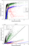 |
Fig. 4 Column densities of the main ice constituents computed with the dynamical model as a function of column density for core 0, shown in the upper panel. Lower panel shows the same figure but with an axis setting similar to Fig. 7 of Boogert et al. (2015). The straight lines are the observed linear relations found by Boogert et al. (2015). |
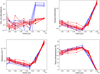 |
Fig. 5 CO2 ice abundance (upper left panel), visual extinction (upper right panel), H2 density (lower left panel), and dust temperature (lower right panel) as a function of time for a few cells. The blue curves present the results for the “high CO2 column density cases” while the red ones are the “low CO2 column density cases.” |
5 Static versus dynamical models
The two sets of models (static and dynamical) present very different approaches. The static simulations are based on the observed conditions in a specific cloud (L429-C) and compared to the ice composition observed toward a few lines of sight in this region. The dynamical simulations are based on time dependent physical conditions computed using a SPH model and compared to observations gathered in the literature for various clouds. As such the physical conditions (density and gas temperature) have been computed along evolutionary paths leading to a variety of local density and gas temperatures for a given visual extinction (see Fig. B.1). The observed spread at a single visual extinction is thus not linked to model uncertainty but related to the various possible chemical trajectories as discussed below. The densities in the dynamical simulations is higher than in the static models, while the gas temperature is smaller. We note that the gas temperature (within the ranges considered here) has little impact on the ice composition. For the static and dynamical simulations using Hocuk’s approximation, the dust temperature is the same at a given AV. The range of visual extinctions scanned for both sets of simulations is not the same. The static models only probe visual extinctions larger than 5 (up to 76) while the dynamical simulations start at AV of 3 × 10⁻⁴ (only up to 25). The main differences between the two types of simulations are however the time evolution of the physical conditions (nonexistent for the static models). For this reason, the times of both simulations do have the same meaning. To compare the column densities obtained from both sets of simulations, we plotted them in the same figure (Fig. B.2) for the common range of AV (5 to 25). The two sets of models compared here have the same dust temperature as a function of AV and the same initial composition. The results of the static model are shown for two times: 105 and 106 yr. The dynamical model is shown for the final time and core 0.
The first obvious difference is the spread of molecular column densities obtained from the dynamical simulations for a single value of AV, while the static simulations all give the same column density. This spread is particularly important for CO2. The late time (106 yr) static models seem to fall within the dynamical simulations for H2O and CH3OH. The static simulations always produce too small amounts of CO2 ices (similar or even below some of the dynamical simulations) whatever the time considered. For CO ice, the static simulations produce smaller amounts except at high AV (>15) for which the static simulations are similar to the dynamic ones at late times. Similar conclusions can be drawn when comparing to the dynamical simulations for other cores.
6 Chemistry of CO2
In these simulations, we have not included the formation of CO2 ices though energetic processes such as the irradiation of CO ices by photons, charged particles, or electrons (Gerakines et al. 1996; Palumbo et al. 1998; Jamieson et al. 2006; Ioppolo et al. 2009; Yuan et al. 2014). These processes are particularly efficient in relatively diffuse regions because of the high external vacuum ultraviolet (VUV) flux and so, if anything, they would strengthen our conclusion that CO2 ices are already built before the formation of the cold cores.
In our chemical model, we have included the following production reactions of CO2 ices:
 (2)
(2)
 (3)
(3)
 (4)
(4)
 (5)
(5)
 (6)
(6)
 (7)
(7)
 (8)
(8)
 (9)
(9)
 (10)
(10)
 (11)
(11)
In astrochemical models with large networks, many chemical processes are in competition. At 10 K, reactions (2) and (3), for instance, will end up competing with the hydrogenation of HCO to form CH3OH, which will be much faster than the reaction with atomic oxygen. Reaction (7) (studied by Minissale et al. 2015) is also in competition with the hydrogenation of H2CO (much faster) leading to methanol. The primary formation of HOCO, necessary to reactions (8)–(11), is slow. So the fastest pathways to form CO2 ices will be reactions (4)–(6). Reactions (5) and (6) should be more efficient than reaction (4) because they have a smaller activation barrier: 150 K for reactions (5) and (6) (Fulle et al. 1996) and 627 K for reaction 4 (mean value of the barrier found by Minissale et al. 2013). It should be noted that the comparison is difficult to make, as the barriers for reactions (5) and (6) have been measured only in the gas phase – contrary to reaction (4). OH would however be hydrogenated to form H2O much faster than it can react with CO. For this reason, our simulations do not form CO2 ice when the dust temperature remains at 10 K but mostly H2CO, CO, and CH3OH ices, as shown in Fig. 3.
Based on Goumans & Andersson (2010), Garrod & Pauly (2011) tested the hypothesis that atomic oxygen, once absorbed on the dust surface, would form a special bond with COice and produce a O…COice complex. This complex would then be hydrogenated and quickly react to form CO2ice. This would mimic reaction (4) with a much lower barrier. In this way, Garrod & Pauly (2011) could form significant amounts of CO2 ice. Our model includes such processes, as previously detailed in Ruaud et al. (2015):
 (12)
(12)
 (13)
(13)
 (14)
(14)
This process was switched off in the simulations shown here because of all the uncertainties in the temperature dependence of the existence of the O…COice complex. In Ruaud et al. (2015), the authors found that this process could form significant amounts of CO2 ice if the binding energy of the complex O…COice was greater than 400 K. Their predicted abundance was, however, a few 10−6 and they did not compare quantitatively with observations. In addition, their model was only a two-phase model. In the current three-phase version of nautilus, the formation of O…COice occurs only at the surface of the grains, not the bulk. We tested the effect of this process by switching it on and running the following models: (1) Static models with the physical conditions observed in L429-C except for the dust temperature computed with the Hocuk et al. (2017) approximation. The results are presented in the left and central panels of Fig. 6 and should be compared with Fig. 3. (2) Dynamical model for core 0 with the dust temperature computed with the Hocuk et al. (2017) approximation. The results are presented in the right-hand panel of Fig. 6 and should be compared with Fig. 4.
The effect of these reactions is strong at high visual extinction and, thus, low temperature. The computed column densities of CO2 are much higher in both the static and dynamical simulations. In the case of the static models, the predicted column densities of CO2 are still lower than the observations by several orders of magnitude, especially at low visual extinction. The H2O and CO predicted column densities are unchanged but the methanol columns densities are also increased through the following path:  (pathways added with the O…COice complex from Ruaud et al. 2015). For the dynamical models, the CO2 ice column densities are also increased at high visual extinction, but only in the cases giving low values. This means that the overall CO2 column densities are not increased and that the main paths leading to values close to the observations are still the ones with the appropriate physical conditions at earlier times.
7 Influence of the dust temperature
Whatever model is applied, the dust temperature is always a key parameter. To understand the sensitivity of the model results to this parameter, we reran all our simulations (static and dynamic), adding 1 K to the dust temperatures computed with the Hocuk et al. (2017) approximation (“Hocuk+1”). The dust temperature as a function of visual extinction in that case is shown in green in Fig. 2. The dust temperature of 12 K occurs for a larger visual extinction (4 instead of 2.7) compared to Hocuk value. This change extends the window within which the CO2 can form (Tdust > 12 K and Av > 2). Although there is no proper error bar given with Hocuk’s relation, a departure of one Kelvin from this parametrization is certainly reasonable while comparing the observed dust temperatures at various AV with this relation (see their Fig. 1).
For the static models, results are unchanged. The “Hocuk+1” case, including the O…CO complex, gives similar results to the case Hocuk with the O…CO complex, except that the CO2 column densities are higher at very low Av, but again not at the levels constrained by the observations. The impact on the dynamical simulations are more significant. Figure 7 shows the model results in that case, which should be compared to Fig. 4. A larger number of trajectories produce detectable amounts of CO2. Adding the O…CO complex to this model does not significantly change the results. So for the rest of the paper, we adopt this prescription of the dust temperature.
The effect of the dust temperature on the chemistry rises through the diffusion rates of the species on the grains. In the model, the diffusion rate of each species is proportional to exp(−Ebind/kT) with T as the dust temperature, Ebind as the binding energy of the species, and k as the Boltzmann constant. (Ruaud et al. 2016). The higher the dust temperature or the smaller the binding energy, the higher the diffusion. As discussed in Sect. 3.3, the binding energies of physisorbed species are quite uncertain and very likely vary from one model to another. In addition, the grain surfaces are not homogeneous and the binding energies are better represented by a distribution rather than a single value – as assumed in the models (see for instance Noble et al. 2012; Doronin et al. 2015; Minissale et al. 2022, and references therein).
 |
Fig. 6 Column density of the main ice constituents computed with Nautilus for the static physical conditions as observed in L429-C as a function of visual extinction (left and middle). Model results are shown at 105 yr in the left-hand panel and 106 yr in the central panel. Diamonds represent the column densities observed by Boogert et al. (2011) at specific positions in the core. Column densities of the main ice constituents computed with the dynamical model as a function of column density (right). For all figures, the dust temperature is computed following Hocuk et al. (2017) and the O…COice complex from Ruaud et al. (2015) is included. |
8 Predictions of the ice composition diversity
Among the 12 theoretical cores we studied, we chose to present core 0 in Sect. 4.2 because it presents both trajectories leading to high and low abundances of CO2 ice. In Fig. 8, we show the model results for all the cores (model “Hocuk+1” without the O…CO complex). Each core presents a different result. For instance, core 5 does not have CH3OH ice column densities greater than 1017 cm−2 whatever the visual extinction and it exhibits a low CO ice column density with respect to the other cores. Cores 8 and 9 present large amounts of CH3OH ice and scarcer CO2 ice when the visual extinction increases. Contrary to core 0, core 2 does not have any trajectories producing CO2 column densities lower than 1017 cm−2 for visual extinctions larger than 15, because the increase in density (and, thus, the visual extinction) and the decrease in dust temperature are smoother with time. To quantify the variability of the ice predictions, we computed the mean values of each species and the standard deviation for bins of visual extinctions. These values for each core are shown in Appendix C and Fig. C.1. When the standard deviation (std) is high, the mean value has no real meaning. In all cores, the std is high for all species at low AV (< 4). At high Av, it is mostly CO2 that presents the higher std. All the other species show a small std when AV is larger than 4 (with the exception of the final AV for cores 5, 6, and 10 for which there are small numbers of points). Interestingly, some of the cores (core 2, 6, 7, and 10) also show a small std of CO2 at high AV.
To take a different perspective on our model results, we show in Fig. 9 the percentage of the main ice constituents with respect to the water abundance as a function of visual extinction for core 2. For all species, the percentage increases rapidly with AV until it reaches a plateau at approximately AV = 5. Such a result is also found for the abundance of these species with respect to the total proton density. One difficulty in addressing these results is the variability of the ice composition with the local physical conditions and their history. All species present a spread in their percentage at a specific visual extinction. While this spread seems to decrease with AV (except for CO2), this could be an effect of having less data. We know that CO2 is the species that presents the largest dispersion in the percentage with respect to H2O. For AV between 10 and 20, the CO2 percentage is approximately between 1 and 50%, the CO percentage between 18 and 115% (although only a very small number of points is responsible for the smallest values), the CH3OH percentage is between 6 and 20%, the NH3 percentage is between 3 and 29%, and the CH4 percentage is between 13 and 34%. We note that the range of percentages are in good agreement with the observed trends, except for CO, which is predicted to be more abundant than water in some cases. These percentages are rather constant with the visual extinction, although variations can exist due to the spread in values. One limitation of our work is that none of our simulations go beyond an AV of 25 because the physical simulations do not include self-gravity. So extrapolations to high visual extinctions are not possible. Figure 7 of Boogert et al. (2015), shows an increase in all ice components that appears to be constant with AV. Our model beyond AV 5 reproduces this feature well. Indeed, having a similar proportion of each component results in a linear evolution of the column density as a function of the visual extinction.
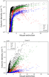 |
Fig. 7 Column densities of the main ice constituents computed with the dynamical model as a function of column density for the “Hocuk+1” model (upper panel). Same figure but with an axis setting similar to Fig. 7 of Boogert et al. (2015) for the “Hocuk+1” model (lower panel). |
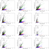 |
Fig. 8 Column densities of the main ice constituents computed with the dynamical model for 12 cores as a function of column density, using the dust temperature approximation “Hocuk+1”. |
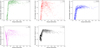 |
Fig. 9 Predicted ice composition (percentage with respect to H2O ice) as a function of visual extinction for core 2 for all trajectories with a water column density greater than 1017 cm−2. |
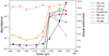 |
Fig. 10 Abundances (with respect to H) of the main ice constituents and gas-phase CO as a function of time. The model is core 2, cell 8 (a trajectory that produced large amounts of CO2 ices). The visual extinction for this simulation is shown in black (dotted line). |
9 Time-dependent formation of ices
In all the figures of column density as function of visual extinction shown up to now for the dynamical models, several timelines are mixed. In this section, we discuss the ice composition as a function of time for one trajectory of core 2 forming large amounts of CO2 ice at high AV. In Fig. 10, we show the abundance of the main ice constituents as a function of time for this cell, zoomed on the time axis to cover the maximum density peak. On the same figure, we show the increase of visual extinction with time. To compare the formation of the ices with the depletion of gas-phase CO, we also plot the CO gas-phase abundance as a function of time. In this example, ice formation becomes efficient within one time step (of 2 × 10⁵ yr, when the visual extinction becomes larger than two). All of the ice constituents but CO form mainly prior to the CO catastrophic freeze-out onto the grains. Then, in the next time step, CO freezes out onto the grains producing a large amount of CO ice. The other ice constituents also increase slightly during this time, except for CO2, whose abundance decreases. This result is in agreement with the proposed evolution sequence of ices by Öberg et al. (2011).
10 Conclusions
We conducted a theoretical study of the formation of interstellar ices at various visual extinctions. Our goal was to reproduce features currently revealed by the observations as well as to make predictions for future JWST results. We carried out two types of simulations. The first was a classic application of an astrochemical model (static model). We used the observed physical conditions from a specific region (cold core L429, probing visual extinctions from 7 to 75) and ran the chemical model for these fixed conditions for a period of time representative of cold cores. One key parameter was revealed to be the dust temperature. When the dust temperature is higher than 12 K, CO2 forms efficiently to the detriment of H2O, while at temperatures below 12 K, CO2 does not form. Whatever our hypothesis on the chemistry, the static simulations failed to reproduce the observed trends of interstellar ices.
When considering the time-dependent physical conditions experienced by interstellar matter forming cold cores (dynamical simulations), we were able to qualitatively reproduce the observations. For these sets of models, we computed the chemistry using time dependent physical conditions from a 3D SPH model of core formation. We studied the formation trajectories of 12 cores, each sampled by tens to hundreds of cells of independent material. We found that a large fraction of the ice was built very early during the formation of the core (especially the CO2 ice) but also that the ice fraction keeps evolving until the density of the core is reached. Large amounts of H2O, CH3OH, NH3, and CH4 are formed on the grains before the catastrophic freeze-out of CO and their abundance keeps increasing afterward. On the contrary, CO2 seems to be mostly formed prior to freeze-out and can even decrease when large amounts of CO stick to the grains. One important result of this study is that efficient formation of CO2 ices requires very specific conditions: a dust temperature greater than 12 K and a visual extinction higher than 2. In our simulations, these conditions are met for a limited number of trajectories and some of our cores never experience them. Considering the ubiquity of CO2 ices, this would appear to be a strong constraint on physical models of the evolution of interstellar matter.
From a chemical point of view, we investigated the various formation pathways of CO2 ice (including the formation of O…CO complex on interstellar grains) and concluded that the COice + Oice reaction at the surface of the grain remains the dominant pathway, despite the slow diffusion of atomic oxygen and the activation barrier to this reaction.
When comparing the static and dynamical simulations, we found that they could produce similar H2O and CH3OH column densities for an integration time of 106 yr of the static models and visual extinction between 5 and 25 (the range of conditions probed by both sets of simulations). For early times, the static models give much smaller column densities. The dynamical simulations produce larger column densities of CO for AV smaller than approximately 15 than the static ones while they give similar results than the static model for 106 yr for larger AV. Last, the static model produces low column densities of CO2 ices, similarly to the low CO2 cases of the dynamic models. This comparison underlines again the need to follow the chemistry during the formation of the clouds, which should happen smoothly. One limitation of our dynamical simulations is that they do not probe the high (AV > 25) visual extinction zone. This is an intrinsic limitation of the physical model that we are using. We however found that percentage of CO, CH3OH, NH3, and CH4 with respect to water was constant for AV larger than 5. Considering that the observational results are based on a very small statistical sample and that our simulations are representative – but still do not reproduce the exact formation trajectories of each observed regions – we conclude that our simulations reproduce the observations well. The large statistical sample, which will be provided by JWST will test the model results and provide new constraints to iteratively improve the simulations.
Acknowledgements
The authors acknowledge the CNRS program “Physique et Chimie du Milieu Interstellaire” (PCMI) co-funded by the Centre National d’Etudes Spatiales (CNES). The authors are grateful to Ian Bonnell for providing the SHP numerical simulations.
Appendix A Observed physical conditions in L429-C
In Fig A.1, we present the physical conditions for the cold core L429 that we used in the static simulations shown in Section 3.
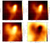 |
Fig. A.1 H2 column density (cm−2), H2 volume density (cm−3), visual extinction, and dust temperature maps of the L429-C region. |
Appendix B Physical conditions and column densities comparison between static and dynamic simulations
In Fig. B.1, we compare the density and gas temperatures used in both sets of simulations (static and dynamical) over the common range of visual extinctions. From these simulations, the computed column densities of the main ice components (H2O, CO2, CO, and CH3OH) as a function of AV is shown in Fig. B.2. Two different times are shown for the static models 105 and 106 yr.
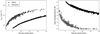 |
Fig. B.1 H density and gas temperature as a function of visual extinction for the static model (same as Fig. 3, black dots) and for the dynamical model of core 0 (same as Fig. 4, gray dots). For both simulations, the grain temperature is computed with Hocuk’s formula as a function of visual extinction. |
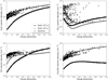 |
Fig. B.2 Icy molecule column densities as a function of visual extinction for the static model (same as Fig. 3, black dots: 105 yr, gray dots: 106 yr) and for the dynamical model of core 0 (same as Fig. 4, black stars). For both simulations, the grain temperature is computed with Hocuk’s formula as a function of visual extinction. |
Appendix C Standard deviation of predicted ice column densities
From the dynamical models presented in section 8 (using the “Hocuk+1” approximation for the dust temperature), we computed, for each core and each of the species H2O, CO2, CO, and CH3OH, the mean column densities and the std for bins of visual extinctions (< 2,2-4,4-6,6-8, 8-10,10-15, and > 15). In the case of a very large dispersion at a specific AV range, the std is very high and the mean values have no meaning. Some of the large std at high AV are due to a small number of statistical points (for instance core 6 at AV 12.5).
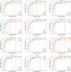 |
Fig. C.1 Mean column densities and standard deviations as a function of AV for each core and the main ice constituents. |
References
- Bergin, E. A., Hartmann, L. W., Raymond, J. C., & Ballesteros-Paredes, J. 2004, ApJ, 612, 921 [NASA ADS] [CrossRef] [Google Scholar]
- Bonnell, I. A., Dobbs, C. L., & Smith, R. J. 2013, MNRAS, 430, 1790 [NASA ADS] [CrossRef] [Google Scholar]
- Boogert, A. C. A., Huard, T. L., Cook, A. M., et al. 2011, ApJ, 729, 92 [NASA ADS] [CrossRef] [Google Scholar]
- Boogert, A. C. A., Gerakines, P. A., & Whittet, D. C. B. 2015, ARA&A, 53, 541 [Google Scholar]
- Bron, E., Daudon, C., Pety, J., et al. 2018, A&A, 610, A12 [CrossRef] [EDP Sciences] [PubMed] [Google Scholar]
- Chang, Q., Cuppen, H. M., & Herbst, E. 2007, A&A, 469, 973 [NASA ADS] [CrossRef] [EDP Sciences] [Google Scholar]
- Congiu, E., Sow, A., Nguyen, T., Baouche, S., & Dulieu, F. 2020, Rev. Sci. Instrum., 91, 124504 [NASA ADS] [CrossRef] [Google Scholar]
- Daranlot, J., Hincelin, U., Bergeat, A., et al. 2012, PNAS, 109, 10233 [NASA ADS] [CrossRef] [Google Scholar]
- Doronin, M., Bertin, M., Michaut, X., Philippe, L., & Fillion, J. H. 2015, J. Chem. Phys., 143, 084703 [NASA ADS] [CrossRef] [Google Scholar]
- Draine, B. T. 1978, ApJS, 36, 595 [Google Scholar]
- Fulle, D., Hamann, H. F., Hippler, H., & Troe, J. 1996, J. Chem. Phys., 105, 983 [NASA ADS] [CrossRef] [Google Scholar]
- Garrod, R. T., & Pauly, T. 2011, ApJ, 735, 15 [Google Scholar]
- Garrod, R. T., Wakelam, V., & Herbst, E. 2007, A&A, 467, 1103 [NASA ADS] [CrossRef] [EDP Sciences] [Google Scholar]
- Gerakines, P. A., Schutte, W. A., & Ehrenfreund, P. 1996, A&A, 312, 289 [NASA ADS] [Google Scholar]
- Goto, M., Bailey, J. D., Hocuk, S., et al. 2018, A&A, 610, A9 [EDP Sciences] [Google Scholar]
- Goumans, T. P. M., & Andersson, S. 2010, MNRAS, 406, 2213 [NASA ADS] [CrossRef] [Google Scholar]
- Graedel, T. E., Langer, W. D., & Frerking, M. A. 1982, ApJS, 48, 321 [NASA ADS] [CrossRef] [Google Scholar]
- Hasegawa, T. I., & Herbst, E. 1993, MNRAS, 261, 83 [NASA ADS] [CrossRef] [Google Scholar]
- Hasegawa, T. I., Herbst, E., & Leung, C. M. 1992, ApJS, 82, 167 [Google Scholar]
- He, J., Shi, J., Hopkins, T., Vidali, G., & Kaufman, M. J. 2015, ApJ, 801, 120 [NASA ADS] [CrossRef] [Google Scholar]
- Herbst, E., & van Dishoeck, E. F. 2009, ARA&A, 47, 427 [NASA ADS] [CrossRef] [Google Scholar]
- Hincelin, U., Wakelam, V., Hersant, F., et al. 2011, A&A, 530, A61 [NASA ADS] [CrossRef] [EDP Sciences] [Google Scholar]
- Hincelin, U., Chang, Q., & Herbst, E. 2015, A&A, 574, A24 [NASA ADS] [CrossRef] [EDP Sciences] [Google Scholar]
- Hocuk, S., SzUcs, L., Caselli, P., et al. 2017, A&A, 604, A58 [NASA ADS] [CrossRef] [EDP Sciences] [Google Scholar]
- Ioppolo, S., Palumbo, M. E., Baratta, G. A., & Mennella, V. 2009, A&A, 493, 1017 [NASA ADS] [CrossRef] [EDP Sciences] [Google Scholar]
- Ioppolo, S., Cuppen, H. M., Romanzin, C., van Dishoeck, E. F., & Linnartz, H. 2010, Phys. Chem. Chem. Phys., 12, 12065 [Google Scholar]
- Jamieson, C. S., Mebel, A. M., & Kaiser, R. I. 2006, ApJS, 163, 184 [NASA ADS] [CrossRef] [Google Scholar]
- Jenkins, E. B. 2009, ApJ, 700, 1299 [Google Scholar]
- McClure, M., Bailey, J., Beck, T., et al. 2017, IceAge: Chemical Evolution of Ices during Star Formation, JWST Proposal ID 1309. Cycle 0 Early Release Science [Google Scholar]
- McClure, M. K., Rocha, W. R. M., Pontoppidan, K. M., et al. 2023, Nat. Astron., 7, 431 [NASA ADS] [CrossRef] [Google Scholar]
- Minissale, M., & Dulieu, F. 2014, J. Chem. Phys., 141, 014304 [NASA ADS] [CrossRef] [Google Scholar]
- Minissale, M., Congiu, E., Manicò, G., Pirronello, V., & Dulieu, F. 2013, A&A, 559, A49 [NASA ADS] [CrossRef] [EDP Sciences] [Google Scholar]
- Minissale, M., Loison, J. C., Baouche, S., et al. 2015, A&A, 577, A2 [NASA ADS] [CrossRef] [EDP Sciences] [Google Scholar]
- Minissale, M., Congiu, E., & Dulieu, F. 2016a, A&A, 585, A146 [NASA ADS] [CrossRef] [EDP Sciences] [Google Scholar]
- Minissale, M., Dulieu, F., Cazaux, S., & Hocuk, S. 2016b, A&A, 585, A24 [NASA ADS] [CrossRef] [EDP Sciences] [Google Scholar]
- Minissale, M., Aikawa, Y., Bergin, E., et al. 2022, ACS Earth Space Chem., 6, 597 [NASA ADS] [CrossRef] [Google Scholar]
- Murakawa, K., Tamura, M., & Nagata, T. 2000, ApJS, 128, 603 [Google Scholar]
- Neufeld, D. A., & Wolfire, M. G. 2017, ApJ, 845, 163 [Google Scholar]
- Neufeld, D. A., Wolfire, M. G., & Schilke, P. 2005, ApJ, 628, 260 [Google Scholar]
- Noble, J. A., Congiu, E., Dulieu, F., & Fraser, H. J. 2012, MNRAS, 421, 768 [NASA ADS] [Google Scholar]
- Noble, J. A., Fraser, H. J., Aikawa, Y., Pontoppidan, K. M., & Sakon, I. 2013, ApJ, 775, 85 [Google Scholar]
- Noble, J. A., Fraser, H. J., Pontoppidan, K. M., & Craigon, A. M. 2017, MNRAS, 467, 4753 [Google Scholar]
- Öberg, K. I., Boogert, A. C. A., Pontoppidan, K. M., et al. 2011, ApJ, 740, 109 [Google Scholar]
- Padovani, M., Bialy, S., Galli, D., et al. 2022, A&A, 658, A189 [NASA ADS] [CrossRef] [EDP Sciences] [Google Scholar]
- Palumbo, M. E., Baratta, G. A., Brucato, J. R., et al. 1998, A&A, 334, 247 [Google Scholar]
- Pontoppidan, K. M., van Dishoeck, E. F., & Dartois, E. 2004, A&A, 426, 925 [NASA ADS] [CrossRef] [EDP Sciences] [Google Scholar]
- Ruaud, M., Loison, J. C., Hickson, K. M., et al. 2015, MNRAS, 447, 4004 [Google Scholar]
- Ruaud, M., Wakelam, V., & Hersant, F. 2016, MNRAS, 459, 3756 [Google Scholar]
- Ruaud, M., Wakelam, V., Gratier, P., & Bonnell, I. A. 2018, A&A, 611, A96 [NASA ADS] [CrossRef] [EDP Sciences] [Google Scholar]
- Ruffle, D. P., & Herbst, E. 2001, MNRAS, 324, 1054 [NASA ADS] [CrossRef] [Google Scholar]
- Sadavoy, S. I., Keto, E., Bourke, T. L., et al. 2018, ApJ, 852, 102 [NASA ADS] [CrossRef] [Google Scholar]
- Stutz, A. M., Bourke, T. L., Rieke, G. H., et al. 2009, ApJ, 690, L35 [NASA ADS] [CrossRef] [Google Scholar]
- Taillard, A., Wakelam, V., Gratier, P., et al. 2023, A&A, 670, A141 [NASA ADS] [CrossRef] [EDP Sciences] [Google Scholar]
- Vasyunin, A. I., Caselli, P., Dulieu, F., & Jiménez-Serra, I. 2017, ApJ, 842, 33 [Google Scholar]
- Wagenblast, R., & Hartquist, T. W. 1989, MNRAS, 237, 1019 [NASA ADS] [Google Scholar]
- Wakelam, V., & Herbst, E. 2008, ApJ, 680, 371 [NASA ADS] [CrossRef] [Google Scholar]
- Wakelam, V., Loison, J. C., Herbst, E., et al. 2015, ApJS, 217, 20 [NASA ADS] [CrossRef] [Google Scholar]
- Wakelam, V., Bron, E., Cazaux, S., et al. 2017a, Mol. Astrophys., 9, 1 [Google Scholar]
- Wakelam, V., Loison, J. C., Mereau, R., & Ruaud, M. 2017b, Mol. Astrophys., 6, 22 [NASA ADS] [CrossRef] [Google Scholar]
- Wakelam, V., Ruaud, M., Gratier, P., & Bonnell, I. A. 2019, MNRAS, 486, 4198 [NASA ADS] [CrossRef] [Google Scholar]
- Wakelam, V., Iqbal, W., Melisse, J. P., et al. 2020, MNRAS, 497, 2309 [NASA ADS] [CrossRef] [Google Scholar]
- Wakelam, V., Dartois, E., Chabot, M., et al. 2021, A&A, 652, A63 [NASA ADS] [CrossRef] [EDP Sciences] [Google Scholar]
- Ward, M. D., Hogg, I. A., & Price, S. D. 2012, MNRAS, 425, 1264 [NASA ADS] [CrossRef] [Google Scholar]
- Yang, Y.-L., Green, J. D., Pontoppidan, K. M., et al. 2022, ApJ, 941, L13 [NASA ADS] [CrossRef] [Google Scholar]
- Yuan, C., Cooke, I. R., & Yates, J., John, T., 2014, ApJ, 791, L21 [NASA ADS] [CrossRef] [Google Scholar]
Note: the original maps from Taillard et al. (2023) contained 79 × 79 pixels. We resampled them to compute the chemistry over fewer spatial points.
All Tables
All Figures
|
Fig. 1 Column density of the main ice constituents computed with Nautilus for the static physical conditions as observed in L429-C as a function of visual extinction (derived from Herschel observations). Diamonds represent the observed column densities by Boogert et al. (2011) on specific positions of the cloud. The model result at two different times are shown: 105 yr on the left and 106 yr on the right. The dust temperature is equal to that observed by Herschel. |
| In the text | |
|
Fig. 2 Dust temperature as a function of visual extinction used for the models. In black: dust temperature measured by Herschel. In gray: dust temperature computed with Hocuk et al. (2017) approximation. In green: dust temperature computed with Hocuk et al. (2017) approximation plus 1 K (“Hocuk+1”). |
| In the text | |
|
Fig. 3 Same as Fig. 1 but for the models in which the dust temperature is computed with the Hocuk et al. (2017) approximation (rather than the temperature derived from Herschel observations). |
| In the text | |
|
Fig. 4 Column densities of the main ice constituents computed with the dynamical model as a function of column density for core 0, shown in the upper panel. Lower panel shows the same figure but with an axis setting similar to Fig. 7 of Boogert et al. (2015). The straight lines are the observed linear relations found by Boogert et al. (2015). |
| In the text | |
|
Fig. 5 CO2 ice abundance (upper left panel), visual extinction (upper right panel), H2 density (lower left panel), and dust temperature (lower right panel) as a function of time for a few cells. The blue curves present the results for the “high CO2 column density cases” while the red ones are the “low CO2 column density cases.” |
| In the text | |
|
Fig. 6 Column density of the main ice constituents computed with Nautilus for the static physical conditions as observed in L429-C as a function of visual extinction (left and middle). Model results are shown at 105 yr in the left-hand panel and 106 yr in the central panel. Diamonds represent the column densities observed by Boogert et al. (2011) at specific positions in the core. Column densities of the main ice constituents computed with the dynamical model as a function of column density (right). For all figures, the dust temperature is computed following Hocuk et al. (2017) and the O…COice complex from Ruaud et al. (2015) is included. |
| In the text | |
|
Fig. 7 Column densities of the main ice constituents computed with the dynamical model as a function of column density for the “Hocuk+1” model (upper panel). Same figure but with an axis setting similar to Fig. 7 of Boogert et al. (2015) for the “Hocuk+1” model (lower panel). |
| In the text | |
|
Fig. 8 Column densities of the main ice constituents computed with the dynamical model for 12 cores as a function of column density, using the dust temperature approximation “Hocuk+1”. |
| In the text | |
|
Fig. 9 Predicted ice composition (percentage with respect to H2O ice) as a function of visual extinction for core 2 for all trajectories with a water column density greater than 1017 cm−2. |
| In the text | |
|
Fig. 10 Abundances (with respect to H) of the main ice constituents and gas-phase CO as a function of time. The model is core 2, cell 8 (a trajectory that produced large amounts of CO2 ices). The visual extinction for this simulation is shown in black (dotted line). |
| In the text | |
|
Fig. A.1 H2 column density (cm−2), H2 volume density (cm−3), visual extinction, and dust temperature maps of the L429-C region. |
| In the text | |
|
Fig. B.1 H density and gas temperature as a function of visual extinction for the static model (same as Fig. 3, black dots) and for the dynamical model of core 0 (same as Fig. 4, gray dots). For both simulations, the grain temperature is computed with Hocuk’s formula as a function of visual extinction. |
| In the text | |
|
Fig. B.2 Icy molecule column densities as a function of visual extinction for the static model (same as Fig. 3, black dots: 105 yr, gray dots: 106 yr) and for the dynamical model of core 0 (same as Fig. 4, black stars). For both simulations, the grain temperature is computed with Hocuk’s formula as a function of visual extinction. |
| In the text | |
|
Fig. C.1 Mean column densities and standard deviations as a function of AV for each core and the main ice constituents. |
| In the text | |
Current usage metrics show cumulative count of Article Views (full-text article views including HTML views, PDF and ePub downloads, according to the available data) and Abstracts Views on Vision4Press platform.
Data correspond to usage on the plateform after 2015. The current usage metrics is available 48-96 hours after online publication and is updated daily on week days.
Initial download of the metrics may take a while.