| Issue |
A&A
Volume 675, July 2023
|
|
|---|---|---|
| Article Number | A146 | |
| Number of page(s) | 27 | |
| Section | Stellar atmospheres | |
| DOI | https://doi.org/10.1051/0004-6361/202345985 | |
| Published online | 14 July 2023 | |
Implications of time-dependent molecular chemistry in metal-poor dwarf stars
Zentrum für Astronomie der Universität Heidelberg,
Landessternwarte, Königstuhl 12,
69117
Heidelberg, Germany
e-mail: sdeshmukh@lsw.uni-heidelberg.de
Received:
24
January
2023
Accepted:
17
April
2023
Context. Binary molecules such as CO, OH, CH, CN, and C2 are often used as abundance indicators in stars. These species are usually assumed to be formed in chemical equilibrium. The time-dependent effects of hydrodynamics can affect the formation and dissociation of these species and may lead to deviations from chemical equilibrium.
Aims. We aim to model departures from chemical equilibrium in dwarf stellar atmospheres by considering time-dependent chemical kinetics alongside hydrodynamics and radiation transfer. We examine the effects of a decreasing metallicity and an altered C/O ratio on the chemistry when compared to the equilibrium state.
Methods. We used the radiation-(magneto)hydrodynamics code CO5BOLD and its own chemical solver to solve for the chemistry of 14 species and 76 reactions. The species were treated as passive tracers and were advected by the velocity field. The steady-state chemistry was also computed to isolate the effects of hydrodynamics.
Results. In most of the photospheres in the models we present, the mean deviations are smaller than 0.2 dex, and they generally appear above log τ = −2. The deviations increase with height because the chemical timescales become longer with decreasing density and temperature. A reduced metallicity similarly results in longer chemical timescales and in a reduction in yield that is proportional to the drop in metallicity; a decrease by a factor 100 in metallicity loosely corresponds to an increase by factor 100 in chemical timescales. As both CH and OH are formed along reaction pathways to CO, the C/O ratio means that the more abundant element gives faster timescales to the constituent molecular species. Overall, the carbon enhancement phenomenon seen in very metal-poor stars is not a result of an improper treatment of molecular chemistry for stars up to a metallicity as low as [Fe/H] = −3.0.
Key words: hydrodynamics / stars: abundances / stars: chemically peculiar / stars: atmospheres
© The Authors 2023
 Open Access article, published by EDP Sciences, under the terms of the Creative Commons Attribution License (https://creativecommons.org/licenses/by/4.0), which permits unrestricted use, distribution, and reproduction in any medium, provided the original work is properly cited.
This article is published in open access under the Subscribe to Open model. Subscribe to A&A to support open access publication.
1 Introduction
Stellar atmospheres are generally assumed to preserve the makeup of their birth environment. The abundance of elements heavier than helium (known as metals) in a stellar atmosphere is an indication of the stellar age, with older stars being deficient in metals. Spectroscopy is one of the foremost tools in determining the abundances of various elements in stellar atmospheres. Since the first studies on solar abundances in the 1920s (Payne 1925; Unsöld 1928; Russell 1929) to modern large-scale surveys such as the Gaia-ESO survey (Gilmore et al. 2012), Gaia (Gaia Collaboration 2023), GALAH (Bland-Hawthorn & Sharma 2016), and Pristine (Starkenburg et al. 2017), to name a few, spectroscopically determined stellar parameters have been a key tool in understanding the composition of stellar atmospheres. Instrumentation and modelling have been refined in tandem, with improvements such as the treatment of departure from local thermodynamic equilibrium (LTE) and advancements in one-dimensional (1D) and three-dimensional (3D) model atmospheres. These directly lead to improvements in the determination of solar and stellar abundances because the methods for doing so often rely on model atmospheres and the assumptions therein. As a core component of Galactic archaeology, abundance determinations of stellar photospheres from spec-troscopy often assume chemical equilibrium (implicitly assumed within the LTE assumption). While LTE studies have been used historically to determine stellar abundances (Asplund 2000; Holweger 2001; Caffau et al. 2011), the accurate treatment of the departure from LTE of level populations (known as radiative NLTE treatment) has been shown to provide more accurate abundances in both solar and stellar photospheres (Wedemeyer 2001; Bergemann et al. 2013; Amarsi et al. 2019b; Mashonkina 2020; Magg et al. 2022).
Molecular features are important in metal-poor (MP) stars because atomic lines are comparatively weak (Beers et al. 1992; Aoki et al. 2013; Yong et al. 2013; Koch et al. 2019). In recent years, increasingly metal-poor stars have been discovered (Beers et al. 1992; Beveridge & Sneden 1994; Aoki et al. 2013; Hughes et al. 2022), with a tendency of a carbon enhancement in their atmospheres (Beers & Christlieb 2005; Sivarani et al. 2006; Carollo et al. 2014; Cohen et al. 2005; Hansen et al. 2016; Lucey et al. 2023). These carbon-enhanced metal-poor (CEMP) stars comprise a large fraction of the low-metallicity tail of the metal-licity distribution function in the Galactic halo (Norris et al. 2007; Susmitha et al. 2020). Although NLTE treatment of spectral lines is becoming more prominent (Bergemann et al. 2013, 2019; Mashonkina 2020), most of the work concerning these abundance determinations is still done under the assumption of chemical equilibrium, that is, that all chemical species are in equilibrium with one another. Most NLTE studies consider radiative NLTE, meaning that the radiation field is not in equilibrium with the local background temperature. This changes the population of energy levels in an atom or molecule. Radiative NLTE is still considered in a time-independent fashion. We instead model the time-dependent chemical processes for a variety of species to investigate the effects of hydrodynamics on molecular formation and dissociation to study whether the carbon enhancement seen at very low metallicities is a real effect or is due to a lack of consideration for time-dependent chemistry.
Chemical species will react with one another in such a manner as to approach thermodynamic equilibrium, given enough time. However, as the rates of these reactions depend strongly on temperature and density (Horn & Jackson 1972), there may be regions in the star in which chemical equilibrium conditions are not met. In the deeper, hotter, collision-dominated layers, chemical species evolve to equilibrium on timescales much faster than other physical timescales in the system. The assumption of chemical equilibrium therefore implies that the chemistry evolves to its equilibrium state faster than other processes can significantly perturb it. In this work, the other physical processes are hydrodynamical, and the key question is whether the chemistry reaches its local thermodynamic equilibrium before the species are advected. Convection in a stellar atmosphere can also lead to compression shocks, which quickly heat material. When chemical kinetics are coupled to these processes, the chemistry evolves on a finite timescale, and a prevalence of these hydro-dynamical effects can push the overall chemistry out of its local equilibrium state.
Metallicity also has a large impact on both the overall structure of the atmosphere and the number densities of the species. At a cursory glance, reducing the metallicity by a factor of 100 immediately results in a reduction by a factor of 100 in the number densities, which naturally results in slower mass-action reaction rates. Relative abundances (especially of C and O) also play a large role in determining the final yield as well as the chemical timescales of different species (Hubeny & Mihalas 2015). As a result of the mass-action rates alone then, the sharp reduction in chemical timescales may cause the chemistry to become out of equilibrium in higher, cooler layers.
Currently, many different codes exist for modelling stellar atmospheres. While 1D atmospheres have been used to great effect (Gustafsson et al. 2008; Allard & Hauschildt 1995), 3D time-dependent modelling is essential for accurately modelling hydrodynamical effects within an atmosphere (Pereira et al. 2013). Codes such as CO5BOLD (Freytag et al. 2012), Stagger (Magic et al. 2013), Bifrost (Gudiksen et al. 2011), MuRAM (Vögler et al. 2005), and Mancha (Khomenko et al. 2017) are prominent examples. We used CO5BOLD model atmospheres to model hydrodynamics, radiation transfer, and time-dependent chemistry together.
We investigate two distinct methods to treat the chemical evolution in a stellar atmosphere. The first is to evolve the chemistry as a post-processing step, using outputs from model atmospheres (known as snapshots) in order to determine the chemical evolution of various species. This method yields accurate results in regimes where the density-temperature profile is conducive to fast-evolving chemistry (in comparison to advec-tion). The second method is to evolve the chemistry alongside the hydrodynamics, which is usually done after advecting the species. While this is much more expensive computationally, it will yield accurate results even in regimes in which the timescales of the chemistry are comparable to the advection timescale. In principle, both approaches are equivalent given a fine enough cadence because the chemical species are treated as passive scalars. In other words, given a fine enough sampling of snapshots, the post-processing method would tend towards the full time-dependent treatment. The post-processing method of evolving species into equilibrium is hence an approximation; using the final abundances calculated with this method as presented here implicitly assumes the formation of these species in chemical equilibrium. It is precisely this assumption that we investigate by comparing these two methods.
Wedemeyer-Böhm et al. (2005) investigated CO in the solar photosphere and chromosphere in 2D, employing a chemical network with 7 species and 27 reactions. Wedemeyer-Böhm et al. (2006) then expanded this into a 3D analysis, showing the formation of CO clouds at higher layers. We build on this further to include an extended chemical network involving 14 species and 83 reactions, and focus on the photospheres of main-sequence turn-off dwarf stars. We investigate CO, CH, C2, CN, and OH in detail because these 5 species are spectroscopically interesting for abundance determinations in MP stars.
The numerical methods and chemical network setup are described in Sect. 2. The results of the three-dimensional simulations for the time-dependent and steady-state calculations are presented in Sect. 3 and discussed in Sect. 4. Our conclusions are given in Sect. 5.
2 Method
2.1 Chemical reaction network
The chemical reaction network (CRN) that describes the system of differential equations builds on the network presented in Wedemeyer-Böhm et al. (2005), extending it to 14 species and 76 reactions. Table 1 describes these reactions along with the parameters of the rate coefficients. Our network is focused on the evolution of CO, CH, C2, CN, and OH through reactions with neutral atomic and bimolecular species. Radiative association, species exchange, two- and three-body reactions, and collisional dissociation are included. Each reaction is given in the modified Arrhenius form, parametrised by the pre-exponential factor α, an explicit temperature dependence ß, and a characterisation of the activation energy γ (see Sect. 2.4 for a more detailed explanation). Some reactions with CO are catalysed reactions and include a characteristic metal M.
The choice of reactions is discussed below. Generally, the CRN was built to analyse the species CO, CH, CN, C2, and OH. As the network presented in Wedemeyer-Böhm et al. (2005) already includes a good treatment of CO, CH, and OH, we supplement this network with reactions taken from the UMIST Astrochemistry Database (McElroy et al. 2013) to model the other molecular species. Only neutral atomic and bimolecular species were considered due to their prevalence compared to other trace molecules, and the storage limitations imposed by considering a full 3D time-dependent treatment. We neglect photodissociation in this network, but we accept that the effects may not be negligible in very optically thin layers. Additionally, as the reactions used here often come from studies in planetary atmospheres and combustion chemistry, the reactions we present are sometimes defined outside of their temperature limits, especially when considering deep photospheric regions. We chose to focus on higher cooler layers for this reason.
Reaction 58. We chose to use the rate that includes only α, instead of the rate that includes explicit temperature dependence. This is because the temperature limits of this reaction are 10–300 K, and including the temperature-dependent rate would lead to a much greater extrapolation due to the comparatively high temperatures in the model atmospheres.
Reactions 116, 133, and 198. For each of these reactions, two rates are presented in the database for temperature limits of 10–300 K, and 300–3000 K. We opted to use the latter rate as the temperature limits are closer to our use case.
Reaction 206. The reaction is defined for the temperature limits 298–3300K and 295–4000 K. We opted to use the latter rate, which includes a higher upper-temperature limit.
Reaction 236. The reaction is defined for the temperature limits 10–500 K and 158–5000 K. We opted to use the latter rate, which includes a higher upper-temperature limit.
Reaction 244. The reaction is defined for the temperature limits 10–294 K and 295–4500 K. We opted to use the latter rate, which includes a higher upper-temperature limit.
A visualisation of the reaction network is shown in Fig. 1. Atomic species are shown in red, key molecular species are shown in blue, and all other molecular species are shown in grey. The full network with all reactions is too complex to show in full detail, so that we chose to highlight the important reactions as edges between nodes. The network is clearly connected, meaning that any node can be reached starting from any other node, but it is not fully connected because every node does not share an edge with every other node. These properties allowed us to find reaction pathways in the reaction network (see Sect. 4.4).
The carbon enhancement phenomenon is represented by a number of molecular carbon features, including the strong CH G-band feature at 4300 Å (Gray & Corbally 2009), the C2 feature at 5636 Å (Green 2013), the Swan bands (C2)at 5635 Å and 5585 Å, and the 3883 Å CN band (Harmer & Pagel 1973). Koch et al. (2019) also used CN features to identify CN-strong and CN-weak stars in globular clusters. Overall, the spectral synthesis in cool carbon stars from 4000–10000 Å shows that the region harbours many CH, CN, and C2 lines.
CO has a very high bond-dissociation energy of 11.16 eV (March & Smith 2001). It is the key stable state within the chemical network. In the regions in which molecular features form, it is energetically favourable to form CO over CH and OH, for instance. CO therefore dictates the relative yield of other carbon- and oxygen-bearing molecules. Generally, C and O will be largely consumed to form CO, and any excess then forms other molecular species. With a C/O ratio lower than 1 (e.g. for solar composition) and at temperatures that allow for molecular formation, most of the carbon is locked into CO, leaving very little to form other carbonic molecules. With a C/O ratio greater than 1 (e.g. certain carbon-enhanced stars), oxygen is instead used up first, and more carbonic molecules form (see Fig. 2).
We included OH to investigate the effect of the C/O ratio on molecular species. OH provides an important symmetry to CH when considering the evolution of C, O, CH, OH, and CO (Gallagher et al. 2016, 2017). As the number of non-CO carbon-bearing molecules heavily depends on the C/O ratio, so too does the evolution of OH.
Reactions used in this work.
 |
Fig. 1 Graph of the chemical reaction network with atoms (red), key molecular species (blue), and remaining molecular species (grey). The connections describe the reaction pathways qualitatively. |
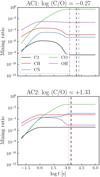 |
Fig. 2 Chemical evolution for two models with [Fe/H] = −3.0, but differing C/O ratios at T = 3500 K, ρ = 10−9 g cm−3 (corresponding to chromospheric background layers). The vertical dash-dotted lines show the time a species has to set into equilibrium. In the oxygen-dominated atmosphere, CH is depleted compared to OH, while the opposite is true in the carbon-dominated atmosphere. |
2.2 Numerical method
We used CO5BOLD, a conservative finite-volume hydrodynamics solver capable of modelling surface convection, waves, shocks, and other phenomena in stellar objects (Freytag et al. 2012). The hydrodynamics, radiation transfer, and chemistry were treated via operator splitting and were solved on a Cartesian grid in a time-dependent manner. The chemistry was solved after the hydrodynamics and radiative transfer time steps. Standard directional splitting along the directions of the 1D operators was used. A Roe solver computed all updates in a single step, where higher-order terms in time are provided based on the applied reconstruction scheme.
Radiative transfer was solved frequency dependently (non-grey) under the LTE assumption using a multiple short-scale characteristic scheme (Steffen 2017). The opacity tables use 12 frequency bins and are consistent with the atomic abundances used for the chemistry input. The model does not treat frequency-dependent photodissociation of chemical species or heating and cooling via reactions. The equation of state is also consistent with the abundances used in the chemistry input and assumes the formation of molecules in instantaneous equilibrium.
All models used in this work were created by taking a thermally relaxed CO5BOLD model output and adding quantity-centred (QUC) quantities (Wedemeyer-Böhm et al. 2005; Freytag et al. 2012). These QUC quantities allow the user to arbitrarily add cell-centred quantities to the simulation. Here, each QUC quantity stores the number densities of a single chemical species across all grid cells. The QUC quantities were advected as prescribed by the velocity field. Periodic boundary conditions were implemented on the lateral edges of the computational domain. The lower boundary layer was open with inflowing entropy and pressure adjustment, while the top layer was transmitting. The number densities in ghost cells were copied from the nearest cells in the computational domain, but were scaled to the mass density of these cells. In this way, the chemistry was still consistent across the boundary, and the number densities of the elements were almost perfectly conserved. We only present 3D models in this work as we focus on the stellar photosphere and it was shown that 1D models are more insensitive to a change in CNO abundances (Plez & Cohen 2005; Gustafsson et al. 2008; Masseron 2008).
The output of the model atmosphere was stored in a sequence of recorded flow properties, commonly called a sequence of snapshots. Each snapshot also functioned as a start model to restart a simulation, or as a template to start a new simulation. To compare the time-dependent chemistry, the same reaction network was solved on a background static snapshot (i.e. a single snapshot without taking advection into account) until the chemistry reached a steady state. This is similar to the treatment of chemistry in equilibrium, but in this case, we still solved the kinetic system instead of relying on equilibrium constants. The method for solving the chemistry independently of the hydrodynamics in post-processing is described in Sect. 2.5.
We used five different 3D model atmospheres that differed in metallicity and chemical composition. A description of the model parameters is given in Table 2. Each model had an effective temperature of 6250 K, a surface gravity of log(g) = 4.00, a resolution of 140 × 140 × 150 cells, and an extent of 26 × 26 × 12.7 Mm (x × y × z). We used standard abundances from the CIFIST grid (Caffau et al. 2011) and initialised the molecular species to a number density of 10−20 g cm−3. The models are referred to in the rest of their work by their ID, namely AM1, AM2, AM3, AC1, and AC2. The models in this study did not use the MHD module and hence represent only quiet stellar atmospheres without magnetic fields.
2.3 Time-dependent chemistry
The radiation-(magneto)hydrodynamics code CO5BOLD includes a time-dependent chemical kinetics solver (Wedemeyer-Böhm et al. 2005; Freytag et al. 2012) that has so far been used to investigate the solar photosphere and chromosphere in two and three dimensions. The code includes modules to advect passive tracers and to solve a chemical reaction network using these passive tracers. Generally, these passive tracers are added to an already thermally relaxed model atmosphere in order to initialise a model with a time-dependent chemistry. When it is initialised, CO5BOLD then solves the chemistry for each cell at each time step (alongside the equations of hydrodynamics and radiation transfer), and the species are advected as prescribed by the velocity field. That is, the time-dependent chemistry for a species ni takes the form
 (1)
(1)
where υ is the velocity field, and S is a source term. The source term is given by the rate of formation and destruction of each species characterised by the reactions in the network.
Each chemical reaction can be written as a differential equation describing the destruction and formation of species, and together, the reactions form an ordinary differential equation (ODE) system. We considered all reactions in this work to follow mass-action kinetics. The rate of a reaction is then given by
 (2)
(2)
where k is the rate coefficient, and the product over nj includes the stoichiometry of either the reactants (forward reaction) or products (reverse reaction). For a generic reaction r with a forward rate coefficient k1 and reverse rate coefficient k2,
 (3)
(3)
the rates of change of the generic species A, B, C, and D in the reaction r are related via
 (4)
(4)
Equation (2) then gives the forward and reverse reaction rates ω1 and ω2 as

respectively. We can then construct the differential  for a species ni and reaction. The full time-dependent chemical evolution of species ni is then given by the sum over the reactions r,
 (5)
(5)
Particle conservation is ensured due to the overall mass continuity equation and the stoichiometry of each chemical reaction. Because only neutral species are considered, no explicit charge conservation is included.
Due to the high computational expense of computing time-dependent chemistry across a large grid, parallelisation is highly recommended. Along with the increased memory load of storing the number densities of QUC species, this limits the size of the network that can be treated time dependently. Even with these steps, solving the chemistry is still the most time-intensive step, taking upwards of 75% of the total runtime.
The DVODE solver (Hindmarsh et al. 2005) was used to solve the system of chemical kinetic equations, making use of the implicit backward differentiation formula (BDF). The solver uses an internally adjusted adaptive time step, which is a requirement when we consider that the system of equations is often very stiff. The solution of the final number densities is provided after the full hydrodynamics time step.
For stability, we used first-order reconstruction schemes for both the hydrodynamics and advection of QUC quantities. Higher-order schemes were found to cause some grid cells to extrapolate beyond the equation-of-state tables or low number densities to become negative. This was not a consistently reproducible effect for a given grid cell, meaning that its source could lie in single-precision numerical errors.
Model atmosphere parameters for the five models used in the study.
2.4 Rate coefficients
The rate coefficient (sometimes rate constant) of a chemical reaction is an often empirically determined quantity dependent on the temperature. Many of the reactions presented in this work are unfortunately defined outside of their temperature limits simply because we lack studies of chemical reactions in high-temperature regions such as stellar photospheric layers. An uncertainty is also associated with the rate coefficients themselves. Despite these shortcomings, the chosen reaction rates are thought to describe the evolution of our species reasonably well.
The Arrhenius rate coefficient is commonly written as
 (6)
(6)
where α is a pre-exponential factor representing the fraction of species that would react if the activation energy Ea were zero, R is the gas constant, and T is the temperature. We used the modified Arrhenius equation, which explicitly includes the temperature dependence
![$k = \alpha \,{\left( {{T \over {300\,\left[ {\rm{K}} \right]}}} \right)^\beta }\,\exp \,\left( { - {\gamma \over T}} \right),$](/articles/aa/full_html/2023/07/aa45985-23/aa45985-23-eq10.png) (7)
(7)
where ß is a fitted constant for a given reaction, and  characterises the activation energy. For a reversible reaction, the forward and reverse coefficients are related to the dimensional equilibrium constant
  by
by
 (8)
(8)
where kf and kr are the forward and reverse rate coefficients, respectively. This equilibrium constant can be used to determine the chemical equilibrium of a given composition, defined when all forward and reverse processes are balanced (Blecic et al. 2016; Stock et al. 2018). As our reaction network contains irreversible reactions in the thermodynamic domain under study, equilibrium constants cannot be determined for each chemical pathway. Hence, we studied the equilibrium chemistry by solving the chemical kinetics until the chemistry reached a steady state. In the absence of processes such as advection, this steady state should correspond to chemical equilibrium.
2.5 Steady-state chemistry
Steady-state chemistry was treated by solving the chemical kinetic system on a background model atmosphere (a single static snapshot), neglecting advection. The chemistry was evolved long enough to reach a steady state in which processes were balanced for each grid cell. The formulation of the final system of equations is the same as that in Eq. (5). In this way, we were able to evaluate the time-dependent effects of advec-tion when compared to the statically post-processed chemistry in steady state.
To solve the chemistry on a background CO5BOLD model snapshot, we present the code called graph chemical reaction network (GCRN)1. GCRN strictly handles a chemical kinetics problem and is able to evaluate the solution at arbitrary times, provided the chemical network, initial number densities, and temperature. The chemistry is solved isothermally in each cell. GCRN is able to read and write chemical network files in the format required by CO5BOLD as well as that of KROME (Grassi et al. 2014). The code is written in Python and primarily relies on the numpy, scipy, and networkx libraries.
The numerical solver is the same as wasused in the time-dependent case, namely DVODE with the BDF method. By default, the absolute tolerance was set to 10−30 and the relative tolerance to 10−4. The Jacobian was computed and evaluated within the DVODE solver itself, but GCRN supports a usersupplied Jacobian matrix. GCRN can also automatically compute an analytical Jacobian based on the equation system and pass this to the solver. Supplying a Jacobian to the solver can help improve stability, but it was not necessary in this work.
GCRN first represents the system of chemical reactions as a weighted, directed graph (see e.g. Horn 1972; van der Schaft et al. 2015). The vertices of the graph are the left and right sides of the chemical reactions, hereafter complexes, while the edges represent the reactions themselves. The weights of the edges are the reaction rates, evaluated for the provided temperature and initial number densities. For a reaction network with c complexes and r reactions, its directed (multi)graph2 G can be characterised by its c × r incidence matrix D, which represents the connection between vertices and edges, that is, which edges connect which vertices. Each column of D corresponds to an edge (a reaction) of G. The (i, j)th element of D represents the reaction j containing complex i. It is +1 if i is a product, and −1 if i is a reactant. For s species, the s × c complex composition matrix Z describes the mapping from the space of complexes to that of species, that is, it describes which species make up which complexes. Multiplying Z and D yields the s × r stoichiometric matrix S = ZD. Finally, to include the mass-action kinetics, we required a vector of reaction rates υ(x) as a function of the species vector x. In general, for a single reaction with a reactant complex C specified by its corresponding column zC = [zC,1 … zC,s]T of Z, the mass action kinetic rate with the rate coefficient k is given by
 (9)
(9)

where ln(x) is defined as an element-wise operation producing the vector [ln(x1)… ln(xs)]T. Similarly, the element-wise operation exp(y) produces the vector [exp(y1)… exp(ys)]T. With this, the mass-action reaction rates of the total network are given by
 (11)
(11)
This can be written compactly in matrix form. We defined the r × c matrix K as the matrix whose ( j, σ)th element is the rate coefficient kj if the σth complex is the reactant complex of the jth reaction, and zero otherwise. Then,
 (12)
(12)
and the mass-action reaction kinetic system can be written as
 (13)
(13)
The formulation is equivalent to that in Eq. (5), with the stoichiometric matrix S = ZD supplying the stoichiometric coefficients and the rate vector υ(x) = K exp(ZT ln(x)) supplying the mass-action kinetic rates. A detailed explanation on the graph theoretical formulation and further analyses can be found in van der Schaft et al. (2016).
A graph theoretical approach allows us to investigate certain behaviours across chemical pathways, such as the timescales of processes and the importance of certain species. These graph representations are only created and accessed upon request and are not used when solving the kinetic system. The graph representations then allow for the analysis of the network in more depth before and after solving the system. In solving the actual kinetic system, only the rates vector υ(x) changes based on the change in number densities. We refer to Sect. 4.4 for an in-depth analysis of the representation of the CRN as a graph.
A drawback of the Python version of GCRN is its low efficiency compared to compiled languages. Although we have implemented a few optimisations, computing the chemical evolution for many snapshots in 3D is still computationally challenging. We therefore used the Julia library Catalyst.3 for steady-state calculations across many 3D snapshots. GCRN was used primarily to evaluate 2D slices, 1D averages, and timescales, while large 3D steady-state calculations were performed in Julia. The results are identical between the two.
3 Results
3.1 Time-dependent versus steady-state chemistry
We investigated the results of time-dependent (TD) chemistry compared to equilibrium (Eqm) chemistry in 3D. For all models, chemical equilibrium is generally held below log τ = 1. Figure 3 shows the absolute number densities and mixing ratios of species across the photosphere for both the time-dependent and steady-state chemistry. The mixing ratio is defined as
 (14)
(14)
where ni is the number density of species i, and ntotal is the number density of all species excluding H, H2, and M. In this way, the mixing ratio describes the relative abundances of important atomic and molecular species in a given volume. H, H2, and M are much more abundant than other species, and including these species simply scales the relevant quantities down. We characterise deviations by considering the ratio of TD to CE mixing ratios, which is equivalent to considering the ratio of TD to CE number densities.
Molecular chemistry is clearly in equilibrium in the deeper photospheric layers, generally below log τ = 1. This is expected because the high temperatures in this collision-dominated regime result in very short timescales (much shorter than characteristic hydrodynamical timescales). In essence, the assumption of chemical equilibrium holds in these regimes. Significant deviations are not present in the AM1 model, but appear above log τ ≈ −2 in model AM2 and above log τ ≈ −1 in model AM3. In all cases in which the deviations are non-zero, the time-dependent chemistry is affected by hydrodynamics such that there is insufficient time to reach a local chemical equilibrium.
As expected, a decreasing metallicity decreases the number of molecular species that can be formed. The deviations from equilibrium molecular number densities increase with decreasing metallicity because the chemical timescales are slower. The largest deviations are seen in C2 and CN in model AM3, where they reach up to 0.15 dex at log τ = −4. The deviations for the other molecules similarly increase with increasing height. These positive deviations are balanced by (smaller) negative deviations in CO. Essentially, there is insufficient time to form the equilibrium yield of CO in these thermodynamic conditions, and the yield of species that would react to form CO is therefore higher.
Differences that are often present around local features such as shocks can be lost in the global picture (averaging over space and time). Even though the chemistry is mostly in equilibrium throughout the atmosphere, investigating cases in which it is out of equilibrium can lead to an understanding of the hydrodynam-ical effects as well as to insights into where approximations of chemical equilibrium break down. Figures 4 and 5 show the time-dependent mixing ratios in a horizontal and vertical slice through the AM3 model atmosphere, respectively.
Figure 4 shows deviations from CE in CN in and around cool features. Mass-action rates depend on temperature, and therefore, cooler cells lead to longer chemical timescales. The instantaneous CE therefore predicts faster dissociation than is possible within the time-dependent scheme. In higher layers, the same reasoning applies, leading to positive deviations in CN, CH, and C2, offset by negative deviations in CO.
The vertical slice in Fig. 5 shows the evolution of chemistry in various layers and highlights a shock in the upper photosphere. Deviations from CE are seen in all species in higher layers, with the shock being the most prominent example. In CE, all molecular species are immediately dissociated, while the time-dependent shows that even in these higher-temperature regions, CO is not so quickly depleted. While it may seem counterintuitive that CO then shows a small negative deviation from CE, the mean amount of CO in the time-dependent case is smaller than that in CE. This is reflected in the positive deviations from CE seen in CH and CN, which, due to mass conservation, are offset by the negative deviation in CO. Additionally, the reverse trend is also true, in that the formation of CO after a shock passes is slower than predicted in CE.
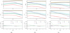 |
Fig. 3 Mixing ratios and deviations from chemical equilibrium for the AM1, AM2, and AM3 models. In the first and second panels, solid lines show the time-dependent quantities, and the hollow points show the equilibrium quantities. Left: [Fe/H] = 0.0. Centre: [Fe/H] = −2.0. Right: [Fe/H] = −3.0. |
3.2 Carbon enhancement
For the models presented thus far, oxygen has been more abundant than carbon. CO, being extremely stable, often dominates the molecular species when it can form. It is possible, however, that this preference towards CO formation is influenced by the enhancement of oxygen relative to carbon present in the atmosphere. We investigated two cases of carbon enhancement in a model atmosphere with metallicity [Fe/H] = −3.0. The first increased both C and O by 2.0 dex (AC1), while the second only increased C by 2.0 dex (AC2). Nitrogen was also increased by 2.0 dex. The increase for all elements included the 0.4 dex enhancement for alpha elements.
Figure 6 shows the mixing ratios and deviations from equilibrium for the two CEMP model atmospheres presented in this work. In model AC1 (log (C/O) = −0.26), more CO and CH is formed than in the standard metal-poor case, but OH is still more abundant than CH. Almost all C is locked up into CO, hence the next most-abundant molecular species is OH. This is analogous to models AM2 and AM3 because O is still more abundant than C. Carbon-bearing molecules are more abundant than in AM3, but the mixing ratios of CH to OH, for example, clearly show that the carbon enhancement does not necessarily lead to a large increase in all carbon-bearing molecular abundances. In model AC2 (C/O = +1.33), CO is still the most abundant species, while CH is more abundant than OH. We observe the opposite effect compared to models AM2, AM3, and AC1, ib which instead O is locked up into CO. This results in a significant depletion of OH compared to model AM3 because there is relatively little O left to form OH because C is overabundant. The depletion of O hinders the formation of further CO, and the chemical equilibrium is such that atomic C is the most abundant species. All models hence reinforce the notion that CO is the most stable molecular state in the chemical network.
Oxygen-bearing species seem to be further out of equilibrium in model AC1, while carbon-bearing species are further out of equilibrium in model AC2. Interestingly, deviations from equilibrium decrease in model AC2, in which the C/O ratio of + 1.33 means that carbon is more abundant than oxygen. While this favours the formation of carbon-bearing species such as C2 and CH, the formation of CO is hindered compared to model AC1 by the lack of OH formation, reinforcing the idea that the pathway for CO formation involving OH is important. The significantly smaller deviations in model AC2 might suggest that oxygen-bearing molecules might show larger deviations from chemical equilibrium due to hydrodynamical effects. All in all, CEMP atmospheres do not seem to be largely out of chemical equilibrium for the species presented in this work.
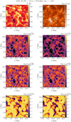 |
Fig. 4 Mixing ratios of molecular species in a horizontal slice through the photosphere in the AM3 model. Left: time dependent. Right: equilibrium. Molecular formation follows a reversed granulation pattern. The effect of finite chemical timescales is most prominent when contrasting warm and cool regions in CN and CH; CO is seen to be relatively close to CE, as confirmed by Fig. 3c at log τ = −4. The white contour traces a temperature of 4500 K. |
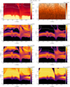 |
Fig. 5 Time-dependent mixing ratios of molecular species in a vertical slice through the photosphere above log τ = 1 in the AM3 model atmosphere. The white contour traces a temperature of 4500 K. The colour scale is the same for all molecular species. |
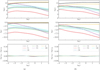 |
Fig. 6 Mixing ratios and deviations from chemical equilibrium at [Fe/H] = −3.0 and a carbon enhancement of +2.0 dex for two atmospheres with different C/O ratios. In the first and second panels, solid lines show the time-dependent quantities, and the hollow points show the equilibrium quantities. Left: model AC1, C/O = −0.26. Right: model AC2, C/O = +1.33. |
4 Discussion
4.1 Effects of convection
As material is transported from hotter, deeper photospheric layers to cooler, higher layers, the conditions for chemistry to equilibriate change. It is feasible, then, that material from a lower layer can be carried upwards, reach a new equilibrium state, and later return to a deeper layer. In this process, molecular species will be present in greater numbers in cooler regions than in hotter regions. If chemistry does not equilibriate faster than advection occurs, we observe deviations from chemical equilibrium throughout convection cells. This effect is seen in Fig. 4 for CN and CH, where features are traced much more sharply in the equilibrium case than in the time-dependent one. The finite chemical timescales are responsible for the differences in formation in cool regions, and dissociation in hot ones. In this layer, the chemical equilibrium approximation still holds well for CO.
4.2 Behaviour around shocks
While the overall differences in time-dependent and steady-state chemistry are small when averaged over time and space (horizontally), there can be significant differences in individual instances in time. In addition to the shock seen in Fig. 5, Fig. 7 shows the deviations from equilibrium molecular chemistry in the photospheres of the AM3, AC1, and AC2 models. This histogram shows deviations from CE binned in gas density and temperature across all 20 snapshots. The top panel gives the bin counts, showing the difference between background material (high density of points) and transient states (low density of points).
Although the background material is generally in equilibrium, three interesting regimes emerge where the molecular chemistry is clearly out of equilibrium, labelled R1, R2, and R3. R1 is the regime of convection in the upper photosphere and chromosphere, where hot material is advected upwards to a new layer faster than the molecular chemistry can reach equilibrium. When this material cools and falls, it can sometimes reach very high velocities (around 10 km s−1) exceeding the local sound speed. This supersonic material of the shock front is captured in the regime R2. Equilibrium chemistry predicts an almost instantaneous dissociation of molecular species, while the time-dependent case models this over a finite timescale. An excess of molecular species is therefore present in the time-dependent case. Finally, the regime R3 is the wake of the shock, where material has cooled and is subsonic. The slower chemical timescales in this regime lead to a depletion of molecular species in the time-dependent case. CO is an outlier here; it is still present in slight excess in R3 as it does not dissociate as quickly as the other molecular species in the shock.
Models AC1 and AC2 show opposite trends in regimes R1 when considering CH, CN, C2, and OH. In model AC1 (logC/O = −0.26), the carbon-bearing molecules are more abundant in the time-dependent case, and OH is depleted. Model AC2 (log C/O = +1.33) instead has fewer carbon-bearing molecules, and OH is more abundant. This is due to the relative abundances of C and O. The chemical timescales depend on the abundances of C and O, so that the oxygen-rich atmosphere AC1 has slower dissociation rates for carbon-bearing molecules but a higher yield because the formation rates for OH are faster (and vice versa for the carbon-rich atmosphere AC2). Since CO is a stable end-product of most reaction pathways, it is not as strongly affected by this phenomenon.
Overall, the differences between the time-dependent and steady-state treatments in the photosphere are small, meaning that the chemistry in convection cells is likely not far from its equilibrium state. This is especially evident when averaging over space and time. However, it is possible that the effects would become stronger in stars on the red giant branch (RGB stars) due to larger scale flows and M-type dwarfs due to cooler temperatures, although the latter have smaller velocity fields, meaning that the effects of advection on the evolution of chemical species are reduced. Wedemeyer-Böhm et al. (2005) showed that the need for time-dependent chemistry becomes increasingly important in the solar chromosphere due to the higher frequency of shock waves alongside lower chemical timescales, but that the photosphere of the Sun was generally in chemical equilibrium for CO. We find the same trend when considering metal-poor dwarf stars: chemical equilibrium generally holds for the photospheres of these stars when we average over space and time, and deviations are largely present in their chromospheres. This further shows the need to include accurate time-dependent molecular chemistry when modelling stellar chromospheres.
4.3 1D analysis
A 1D horizontal cut through the atmosphere shows the instantaneous variations in the parameters and can help identify patterns. Due to mass-action kinetics, the chemical timescales depend on the gas density and temperature. Figure 8 shows profiles of these quantities alongside the time-dependent and equilibrium number densities of CO across a prototypical downflow feature in the chromosphere of model AM3.
The equilibrium CO number density changes much more sharply across the feature than in the time-dependent case. This shows the finite chemical timescales. The number densities are also more sensitive to fluctuations in temperature, as seen towards the end, when the gas density changes but the temperature is constant. The equilibrium number densities show sharp discontinuities due to the vastly different chemical timescales around the shock front. While these are implausible, the average number densities are very similar (as shown in Fig. 3), showing that the shock here is not disruptive enough for CO chemistry to have a profound impact overall.
4.4 Timescales and pathways
It is perceivable that a metallicity reduction by 2.0 leads to timescales that are slower by a factor of ~100 due to the mass action law. Additionally, relative abundances have a strong effect, and the overall yield is lower at lower metallicities. Figure 9 shows the evolution and equilibrium times for three metallicities, and Fig. 2 shows this for the two CEMP models. The equilibrium times for each model and species of interest are given in Table 3. Because of the time-stepping of the solver, these times are not necessarily exact, but they provide a clear picture of how the species interact. The equilibrium times here are generally given as the point at which the relative difference in the number densities falls below a threshold e, that is, teqm is reached when  . We adopted ϵ = 10−6 for this network. Again, because this definition relies on the solver time-stepping to find ni, ni+1, the times are only exact to the times where the solution is evaluated.
The time for each species to reach equilibrium increases with decreasing metallicity. This is a direct consequence of the mass-action kinetics we used to determine reaction rates. The carbon-enhanced models show faster timescales for the same reason.
Another interesting investigation involves the pathways in which molecular species are formed (and disassociated), and how these change throughout the atmosphere. To pursue this, we represent the reaction network as a weighted directed graph, as shown in Sect. 2.5. The nodes are the left and right sides of the reactions (hereafter complexes), and the edges represent the reactions themselves, weighted by their corresponding inverse rate. As this graph is often disconnected, and because we are interested in the species, we added nodes for each individual chemical species. To connect the graph fully, the individual species nodes have an unweighted edge to each complex that contains it. In this way, we can represent the evolution of one species into another by means of the reaction pathways.
We used pathfinding algorithms to move from a source species to a target species, identifying the chemical pathway and its corresponding timescale (simply the sum of the edge weights). These change not only with the temperature, but also with the number densities of the reactants, meaning that the most frequented pathways for a given source-target pair can change during the chemical evolution.
The custom pathfinding algorithm (based on Dijkstra’s shortest-path algorithm; Dijkstra 1959, and taking inspiration from A* pathfinding; Foead et al. 2021) is described in the following steps:
Start on a species source node.
If the current node is the target node, return the path.
Otherwise, find all nodes connected to the current node.
If the last travelled edge had a weight of zero, omit all edges with weights of zero from the next choice of edges.
Pick an edge at random and repeat from 2.
Pathfinding will converge once all possible paths from source to target have been explored.
Step 4 is necessary to prevent species-species jumps that are included as a side effect of adding chemical species to the graph. These unweighted edges are represented with a weight of 0, and traversing two of these consecutively is unphysical (e.g. moving from CO −> CO + H −> H) as it represents a species transforming into another (often completely unrelated) species without a reaction. However, these connections are still necessary to fully connect the graph; we removed the ability to travel along these connections consecutively, effectively altering the graph during pathfinding.
In our network, we investigated key pathways from C and O to CO, as well as the reverse. In all cases, reducing the metallicity resulted in longer timescales for reactions. Additionally, a single reaction dominates in most pathways and is often referred to as the “rate-limiting step” (Tsai et al. 2017, 2018). Table 4 shows the main reactions involved in the formation and dissociation of CO for the AM3 atmosphere. We qualitatively reproduce the same effects as those explored in Wedemeyer-Böhm et al. (2005), and find that of the three reactions that dissociate CO to C and O, the reaction CO → CO + H is by far the most efficient, even in this extremely metal-poor atmosphere. Additionally, formation via species exchange (especially by OH) is the most preferable set of pathways.
We examined the preferred pathways in the network for OH for three abundance mixtures: AM3, AC1, and AC2. AM3 and AC2 are qualitatively similar, where radiative association of OH via H is a leading timescale. Species exchange with CH and CO is not as preferable. AC2 shows exactly the opposite trend, with species exchange routes being significantly better travelled than direct radiative association. Again, this is because in both AM3 and AC2, more free O is available after CO has been formed, while in AC1, very little O is present and OH formation relies on carbonic species.
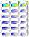 |
Fig. 7 Heat maps of binned quantities for models AM3, AC1, and AC2. Each quantity was binned using 20 snapshots of each 3D model. Deviations from equilibrium are seen in three distinct regions, labelled R1 (convective cells in the upper photosphere), R2 (shock fronts in the chromosphere), and R3 (wake of the shock). |
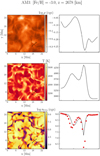 |
Fig. 8 Gas density, temperature, and the number density of CO molecules in a slice across the AM3 atmosphere. The left panels show the 2D heat maps of these quantities, and the right panels show a 1D cut across a prototypical downflow feature, depicted by the solid black line in the top panels. The bottom right panel shows the time-dependent number density as a solid black line and the equilibrium number density as red points. |
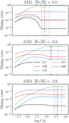 |
Fig. 9 Chemical evolution for three models at differing metallicities at T = 3500 K, ρ = 10−9 g cm−3 (corresponding to the wake of a shock). The vertical dash-dotted lines show the time a species has to set into equilibrium. A reduction in metallicity leads to a corresponding reduction in time to equilibrium and overall yield. |
Time to equilibrium for all models and key molecular species at a temperature of 3500 K and a gas density of 10−9 g cm−3, corresponding to the upper photospheric convection cells.
4.5 Treatment of photochemistry
Our network does not include the effects of photodissociation of species because of the greatly increased complexity required to treat this process properly. In the collision-dominated layers, photochemistry is unlikely to be important, but the situation may be different in higher optically thin layers, where radiation-driven processes become important. The importance of photochemistry is perhaps traced better by the prominence of radiative NLTE effects. The treatment of neutral C in the Sun (Amarsi et al. 2019a) and O in the Sun (Steffen et al. 2015) shows that the abundances are affected up to 0.1 dex in relevant line-forming regions. It is feasible that photochemistry is then an important consideration in higher layers, but the treatment of the photochemical reactions of all atomic and molecular species is a considerably difficult and time-consuming endeavour. We welcome any further advancements in this direction.
4.6 Complexity reduction
Ideally, we would like to include as many species and reactions as possible into the network to model it as precisely as possible. Unfortunately, due to the large memory cost of storing 3D arrays as well as the steep scaling of the solution time with the size of the kinetic system, methods that reduce complexity are often required. In this work, we have presented a heavily reduced network that is focused on the formation and disassociation of a few key molecular species. However, the existence and addition of other species into the network can alter evolution, pathways, and timescales. It is often the case that only a small subset of reactions controls the vast majority of the evolution. Identifying these reactions can prove challenging, but a few methods exist to reduce the complexity of the kinetics problem (Pope 1997; Grassi et al. 2012). In our case, the network was already heavily reduced to the key reactions, and chemical pathways were investigated by Wedemeyer-Böhm et al. (2005), which in part verify this. In the future, we aim to investigate chemical pathways found via a graph theoretical analysis to reduce the number of reactions and species to only those necessary to model significant trends in the regions of interest.
Step-by-step reactions and rate-limiting steps for the AM3 model atmosphere at a temperature of 3500 (K) and a gas density of 10−9 (gcm−3).
4.7 Potential error from LTE assumptions
In the analysis presented thus far, several assumptions have been made that can introduce small errors into the process. It has been demonstrated that the assumption of chemical equilibrium generally holds well in the photospheres of the stars considered in this work. However, deviations increase in higher layers, and several assumptions made about these higher layers should be addressed. Since chemical feedback is neglected, chemical reactions do not affect the temperature of the model atmosphere directly, despite being exo- or endothermic. Furthermore, the equation of state does not take into account the departures from chemical equilibrium. Finally, radiative NLTE corrections may be significant in the higher layers of the atmospheres we consider.
Firstly, the absence of heating and cooling by chemical reactions contributes only a small error. Here we consider the formation of C and O into CO because CO has the highest bond energy of any species presented here and will naturally dominate the effects of chemical feedback due to this property and its abundance. As an extreme case, we considered the conversion of all C into CO in the AM1 atmosphere. This atmosphere is the most metal rich and is oxygen rich, so that this conversion provides an upper limit to the expected change in heat and temperature. The specific heat per unit mass is nearly constant in the upper layers of this atmosphere, with cV ≈ 108 erg g−1 K−1. The formation of CO releases ediss := 11.16 eV (1.79 × 10⁻¹¹ erg) of energy per reaction, and the energy released per mol is found by multiplying by Avogadro’s number. The number fraction of C (where the total amount of species is normalised to unity) divided by the mean molecular weight µ := 1.26 in the neutral stellar atmosphere gives AC ≈ 2.4 × 10⁻⁴. We therefore find the change in temperature
 (15)
(15)
where NA is Avogadro’s number. In the lower-metallicity models presented here, the effect would be significantly smaller. The lack of chemical feedback therefore adds a negligible error to the total energy and temperature.
Secondly, the effects of deviations from equilibrium number densities could have a small effect on the overall structure, but the deviations shown here are relatively small and are generally confined to trace species. The mean molecular weight is dominated by H and He (metals are around ~1%), the deviations of which are completely negligible. Any deviations on the scale seen here would therefore not have significant effects on the overall structure of the model atmosphere.
Thirdly, NLTE radiative transfer may be important when considering chemical kinetics in highly optically thin layers. Popa et al. (2023) showed the importance of this feature on the CH molecule in metal-poor red giant atmospheres, which suggests an increase in measured C abundance compared to LTE techniques (increasing with decreasing metallicity). We find a small increase in CH number density compared to equilibrium values, which would offset the large increase in the LTE carbon abundance required to reproduce the NLTE spectra. Additionally, when the collisional dissociation rates of CH are compared (e.g. Reaction 1), the rates are comparable to or higher than the photodissociation rates across the optically thin atmosphere. We estimated the photodissociation rate of CH with the help of the continuous opacity of provided by Kurucz et al. (1987). For the population numbers, LTE was assumed, and the radiation field of the 1D atmosphere was calculated with opacity distribution functions. The obtained rate suggests overall that photodissociation does not completely dominate the process. It is therefore interesting to consider the interplay between these processes, and we look forward to additional efforts in this field.
Finally, it should be stated that the models presented in this work do not include a comprehensive treatment of the stellar chromosphere. While we note that deviations from chemical equilibrium are important in stellar chromospheres, further work in these areas is therefore necessary and welcome.
5 Conclusion
We have presented a study of 3D time-dependent molecular formation and dissociation in one solar metallicity and four metal-poor atmospheres. The chemistry was modelled through mass-action kinetics with 76 reactions and 14 species that are advected by the velocity field during the hydrodynamics step. We additionally presented a comparison to the equilibrium abundances, computed with Python or Julia chemical kinetics codes. Deviations from equilibrium are seen primarily in higher photo-spheric layers, around shocks, and in the temperature differences throughout convection cells:
In all models presented in this work, molecular species are generally in chemical equilibrium throughout the model photospheres. Molecular species show mean deviations from equilibrium reaching 0.15 in the lower chromosphere, and these deviations increase with decreasing metallicity and increasing height. The largest deviations are in CN, C2, and CH when log (C/O) < 1, and in OH when log (C/O) > 1. Above log τ ≈ −2, the less abundant molecule of C or O becomes locked into CO, inhibiting the formation of other molecular species involving that species. This results in comparatively low amounts of CH, CN, and C2 in all models except AC2, and comparatively low amounts of OH in model AC2;
The deviations from equilibrium can also be attributed to the behaviour around chromospheric shock waves. In the equilibrium case, the hot shock front contains very low number densities of molecular species, while the time-dependent treatment has greater number densities as the evolution proceeds with a finite timescale. In the uppermost coolest layers (T ≤~ 3500 (K)), slow chemical timescales result in a depletion of CO as there is insufficient time to form it before material is advected to a significantly different thermodynamic state;
These deviations are unlikely to contribute significantly to spectroscopic measurements for metal-poor dwarfs because the line cores of key molecular species are generally formed in deeper layers (Gallagher et al. 2017). The largest deviations are mostly outside of the range of the contribution functions for the CH G-band and OH-band, but these deviations could still affect spectral line shapes, which can only be properly reproduced in 3D models. The perceived trend of increased carbon enhancement with decreasing stellar metallicity is therefore not due to an improper treatment of time-dependent chemistry. An investigation including spectrum synthesis using the time-dependent number densities is however warranted in light of these deviations;
Relative deviations increase with decreasing metallicity due to slower mass-action reaction rates. The change in metal-licity does not lead to a strictly linear increase in chemical timescale or decrease in yield in all layers, but generally, lower metallicities result in longer chemical timescales and lower yields;
The C/O ratio plays a key role in determining which molecular species are further out of equilibrium. Both CH and OH are formed along reaction pathways to form CO. In the majority of atmospheres we presented, oxygen is present in excess compared to carbon, making OH formation more viable than CH. This leads to faster chemical timescales for reaction pathways involving OH. Changing this ratio so that carbon is in excess likewise changes the pathways to make the formation of carbon-bearing species preferential;
The lack of chemical feedback contributes a negligible error to the evolution of chemical species, energy, and momentum of the system because these metals are trace species. NLTE radiative transfer has been shown to be of importance in higher layers (Popa et al. 2023), and our deviations point in the opposite direction to those seen through radiative NLTE calculations. Some kinetic rates are as fast or faster than our calculated photodissociation rates across the optically thin atmosphere, suggesting that both radiative NLTE transfer and time-dependent kinetics are important to consider in these layers.
In conclusion, we find molecular species to generally be in a state of chemical equilibrium under photospheric conditions for the models presented in this work. The effect of altering the C/O ratio is directly seen in the final yields of molecular species such as CH and OH. While relative deviations increase with decreasing metallicity because the mass-action kinetic rates are slower, these effects are not large enough to contribute significantly to spectroscopic abundance measurements because the line cores of interest for these stars are generally formed in deeper regions in which chemical equilibrium is well established. The deviations increase with height, and it is likely that there is interesting interplay between radiative and kinetic departures from LTE in the upper photospheres and chromospheres of metal-poor stars.
Acknowledgements
S.A.D. and H.G.L. acknowledge financial support by the Deutsche Forschungsgemeinschaft (DFG, German Research Foundation) –Project-ID 138713538 – SFB 881 (“The Milky Way System”, subproject A04).
Appendix A Carbon enhancement and metallicity
The effect of the C/O ratio can be visualised by investigating reaction pathways between the species C, O, CH, OH, and CO. A simplified reaction network with eight reactions was used in this study, and the temperature dependence was removed from the rate coefficients to investigate the effects of mass-action kinetics. This simplified network takes a subset of reactions from the original network used in this work that characterise the formation and dissociation of CO via CH and OH. In this network, there are two pathways from C and O to CO (and back), shown and labelled in Fig. A.1. The pathway involving C-CH-CO is labelled P1 and that of O-OH-CO is labelled P2. Additionally, the pathways are constructed such that pathways P1 and P2 have the same rates when the amount of C and O is equal. This symmetry allows us to investigate the effect of the C/O ratio alone on the mass-action kinetics. The reaction rates are constant in temperature, but are otherwise constructed to qualitatively match those of the larger network (apart from the symmetry).
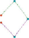 |
Fig. A.1 Diagram of the simplified reaction network showing pathways P1 and P2. |
Fig. A.2 shows the evolution of these species for three cases. Case 1 contains more oxygen than carbon. In case 2, the amount of carbon and oxygen is equal. Case 3 contains more carbon than oxygen. As expected, the overall yield of the number densities reflects that of the input abundances.
We adopted abundances similar to the AM2 model for the three cases. The total timescale was calculated by summing the individual timescales of the reactions along the pathway. The total timescales and abundances considered for each case are shown in Table A.1. The shortest timescales are highlighted in bold. These are not the same timescales as shown in Table 3; the timescales shown there represent the times various species evolve to chemical equilibrium, while the timescales here are inverse reaction rates scaled by number densities. In this sense, they are essentially e-folding timescales.
In case 1, where O is more abundant than C, pathway P2 is faster because forming OH is favourable to forming CH. This results in C and CH being considerably depleted compared to the other species, and it is the same effect as in model AM2. In case 2, where O and C are equally abundant, CH and OH form equally quickly due to the symmetry in the simplified network. In case 3, where C is more abundant than O, the exact opposite behaviour to case 1 is observed (again due to the symmetry), but this is qualitatively similar to model AC2. All in all, the current method allows us to investigate favourable pathways in a given network, validating the chemical species that are especially important when considering the evolution of another. The longer pathways seen here in the simplified network are indicative of similar trends in the full network, reinforcing the notion that as chemical timescales grow longer, approaching dynamical timescales, it becomes increasingly likely that chemical species lie farther from their equilibrium values. However, due to the inclusion of more species and many more pathways between them, the dynamics of the full network are significantly more complicated, and it is not immediately clear from the timescales alone how far species will be out of equilibrium, nor whether they would be present in excess or in depletion. Nevertheless, an analysis of favourable reaction pathways might lead to improvements such as complexity reduction.
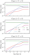 |
Fig. A.2 Evolution of C, CH, CO, O, and OH for a simplified reaction network we used to illustrate the effect of the C/O ratio on equilibrium timescales. |
Total timescales for the C-CH-CO pathway P1 and the O-OH-CO pathway P2 (towards formation of CO) for three different log C/O ratios.
Appendix B Slices through the photosphere
The following figures show horizontal and vertical slices through the photospheres of all models, analogously to Figs. 4 and 5. The slices in the xy direction are all taken at an optical depth of log τ = −4. In all cases, the differences in the xy slices are minor, seen primarily around hot shock fronts where equilibrium chemistry predicts nearly instantaneous dissociation of molecular species, while in the time-dependent case, this proceeds on a finite timescale. The time-dependent molecular species are therefore seen in excess.
In the xz slices, differences are seen in the uppermost layers of the atmosphere (generally only in chromospheric layers). These layers are frequented by shock waves that disrupt molecular formation, and when considering equilibrium chemistry, the effects of molecular dissociation again occur too quickly in the hot shock fronts, and formation of CO occurs too quickly in the cooler regions. As shown in Figs. 9 and 2, molecular formation is very slow (on the order of hours to days), and most molecular species first show an excess in their yield profile before this decreases as they form CO.
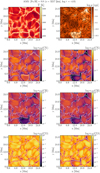 |
Fig. B.1 As Fig. 4, but with [Fe/H] = +0.0. The contour line traces a temperature of 5000 K and highlights areas in which deviations may be present (seen primarily in CN and CO). |
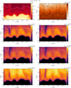 |
Fig. B.2 As Fig. 5, but with [Fe/H] = +0.0. The contour line traces a temperature of 4550 K. Minor deviations are present in the uppermost layers of the atmosphere for CN and CO. |
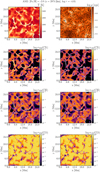 |
Fig. B.3 As Fig. 4, but with [Fe/H] = −2.0. The contour line traces a temperature of 5000 K, highlighting areas in which CN chemistry is out of equilibrium. CH and CO are generally formed under equilibrium conditions. |
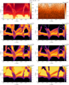 |
Fig. B.4 As Fig. 5, but with [Fe/H] = −2.0. The contour line traces a temperature of 5400 K and highlight hydrodynamical features such as an updraft colliding with a downdraft around x = 6.0 Mm, z = 2.5 Mm. All molecular species are out of equilibrium around this feature as they do not dissociate as quickly as predicted by the equilibrium chemistry. |
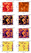 |
Fig. B.5 As Fig. 4, but with a C and O enhancement of +2.0 dex and C/O = −0.27 The contour line traces a temperature of 4900 K. The chemistry is almost entirely in equilibrium in this layer of the atmosphere (due to the enhanced C and O abundances), and minor deviations are visible only for CN around the hotter regions. |
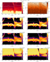 |
Fig. B.6 As Fig. 5, but with a C and O enhancement of +2.0 dex and C/O = −0.27. The contour line traces a temperature of 5150 K and highlights a hot updraft near x = 9.0 Mm where primarily CN and CO molecular dissociation is out of equilibrium. |
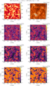 |
Fig. B.7 As Fig. 4, but with a C enhancement of +2.0 dex and C/O = +1.33. The contour line traces a temperature of 5000 K, showing minor deviations present only in CN. The relatively high carbon abundance results in the molecular chemistry being very close to equilibrium conditions. |
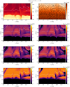 |
Fig. B.8 As Fig. 5, but with a C enhancement of +2.0 dex and C/O = +1.33. The contour line traces a temperature of 4950 K, and the largest deviations are seen in a hot updraft near x = 6.0 Mm, z = 3.0 Mm. The relatively high carbon abundances result in these molecular species being formed very close to equilibrium conditions, although differences are present in these very diluted regions. |
References
- Allard, F., & Hauschildt, P. H. 1995, ApJ, 445, 433 [NASA ADS] [CrossRef] [Google Scholar]
- Amarsi, A. M., Barklem, P. S., Collet, R., Grevesse, N., & Asplund, M. 2019a, A&A, 624, A111 [NASA ADS] [CrossRef] [EDP Sciences] [Google Scholar]
- Amarsi, A. M., Nissen, P. E., Asplund, M., Lind, K., & Barklem, P. S. 2019b, A&A, 622, A4 [NASA ADS] [CrossRef] [EDP Sciences] [Google Scholar]
- Aoki, W., Beers, T. C., Lee, Y. S., et al. 2013, AJ, 145, 13 [CrossRef] [Google Scholar]
- Asplund, M. 2000, A&A, 359, 755 [NASA ADS] [Google Scholar]
- Baulch, D. L., Drysdale, D., Horne, D. G., & Lloyd, A. 1972, Evaluated Kinetic Data for High Temperature Reactions, Vol. 1 [Google Scholar]
- Baulch, D. L., Drysdale, D., Duxbury, J., & Grant, S. J. 1976, Evaluated Kinetic Data for High Temperature Reactions. Homogeneous Gas Phase Reactions of the 02-03 System, the CO-O2-H2 System, and of Sulphur-Containing Species, 1st edn., Vol. 3 (London: Butterworths) [Google Scholar]
- Beers, T. C., & Christlieb, N. 2005, ARA&A, 43, 531 [NASA ADS] [CrossRef] [Google Scholar]
- Beers, T. C., Preston, G. W., & Shectman, S. A. 1992, AJ, 103, 1987 [NASA ADS] [CrossRef] [Google Scholar]
- Bergemann, M., Kudritzki, R.-P., Würl, M., et al. 2013, ApJ, 764, 115 [NASA ADS] [CrossRef] [Google Scholar]
- Bergemann, M., Gallagher, A. J., Eitner, P., et al. 2019, A&A, 631, A80 [NASA ADS] [CrossRef] [EDP Sciences] [Google Scholar]
- Beveridge, R. C., & Sneden, C. 1994, AJ, 108, 285 [NASA ADS] [CrossRef] [Google Scholar]
- Bland-Hawthorn, J., & Sharma, S. 2016, Astron. Nachrichten, 337, 894 [NASA ADS] [CrossRef] [Google Scholar]
- Blecic, J., Harrington, J., & Bowman, M. O. 2016, ApJS, 225, 4 [CrossRef] [Google Scholar]
- Caffau, E., Ludwig, H. G., Steffen, M., Freytag, B., & Bonifacio, P. 2011, Sol. Phys., 268, 255 [Google Scholar]
- Carollo, D., Freeman, K., Beers, T. C., et al. 2014, ApJ, 788, 180 [Google Scholar]
- Cohen, J. G., Shectman, S., Thompson, I., et al. 2005, ApJ, 633, L109 [NASA ADS] [CrossRef] [Google Scholar]
- Dijkstra, E. W. 1959, Numer. Math., 1, 269 [CrossRef] [Google Scholar]
- Foead, D., Ghifari, A., Kusuma, M. B., Hanafiah, N., & Gunawan, E. 2021, Procedia Comput. Sc., 179, 507 [CrossRef] [Google Scholar]
- Freytag, B., Steffen, M., Ludwig, H. G., et al. 2012, J. Comput. Phys., 231, 919 [Google Scholar]
- Gaia Collaboration (Recio-Blanco, A., et al.) 2023, A&A, 674, A38 [CrossRef] [EDP Sciences] [Google Scholar]
- Gallagher, A. J., Caffau, E., Bonifacio, P., et al. 2016, A&A, 593, A48 [NASA ADS] [CrossRef] [EDP Sciences] [Google Scholar]
- Gallagher, A. J., Caffau, E., Bonifacio, P., et al. 2017, A&A, 598, A10 [NASA ADS] [CrossRef] [EDP Sciences] [Google Scholar]
- Gilmore, G., Randich, S., Asplund, M., et al. 2012, The Messenger, 147, 25 [NASA ADS] [Google Scholar]
- Grassi, T., Bovino, S., Gianturco, F. A., Baiocchi, P., & Merlin, E. 2012, MNRAS, 425, 1332 [NASA ADS] [CrossRef] [Google Scholar]
- Grassi, T., Bovino, S., Schleicher, D. R. G., et al. 2014, MNRAS, 439, 2386 [Google Scholar]
- Gray, R., & Corbally, C. 2009, Stellar Spectral Classification (Princeton University Press) [CrossRef] [Google Scholar]
- Green, P. 2013, ApJ, 765, 12 [NASA ADS] [CrossRef] [Google Scholar]
- Gudiksen, B. V., Carlsson, M., Hansteen, V. H., et al. 2011, A&A, 531, A154 [NASA ADS] [CrossRef] [EDP Sciences] [Google Scholar]
- Gustafsson, B., Edvardsson, B., Eriksson, K., et al. 2008, A&A, 486, 951 [NASA ADS] [CrossRef] [EDP Sciences] [Google Scholar]
- Hansen, C. J., Nordström, B., Hansen, T. T., et al. 2016, A&A, 588, A37 [NASA ADS] [CrossRef] [EDP Sciences] [Google Scholar]
- Harmer, D. L., & Pagel, B. E. J. 1973, MNRAS, 165, 91 [NASA ADS] [CrossRef] [Google Scholar]
- Hindmarsh, A. C., Brown, P. N., Grant, K. E., et al. 2005, ACM Trans. Math. Softw., 31, 363 [CrossRef] [Google Scholar]
- Holweger, H. 2001, AIP Conf. Proc., 598, 23 [NASA ADS] [CrossRef] [Google Scholar]
- Horn, F. 1972, Arch. Rational Mech. Anal., 49, 172 [Google Scholar]
- Horn, F., & Jackson, R. 1972, Arch. Rational Mech. Anal., 47, 81 [NASA ADS] [CrossRef] [Google Scholar]
- Hubeny, I., & Mihalas, D. 2015, Theory of Stellar Atmospheres, Princeton Series in Astrophysics (Princeton University Press) [Google Scholar]
- Hughes, A. C. N., Spitler, L. R., Zucker, D. B., et al. 2022, ApJ, 930, 47 [NASA ADS] [CrossRef] [Google Scholar]
- Khomenko, E., Vitas, N., Collados, M., & de Vicente, A. 2017, A&A, 604, A66 [NASA ADS] [CrossRef] [EDP Sciences] [Google Scholar]
- Koch, A., Grebel, E. K., & Martell, S. L. 2019, A&A, 625, A75 [NASA ADS] [CrossRef] [EDP Sciences] [Google Scholar]
- Konnov, A. A. 2000, 28th Symp Int Combust. Edinb., Abstr. Symp. Pap., 317 [Google Scholar]
- Kurucz, R. L., van Dishoeck, E. F., & Tarafdar, S. P. 1987, ApJ, 322, 992 [NASA ADS] [CrossRef] [Google Scholar]
- Lucey, M., Al Kharusi, N., Hawkins, K., et al. 2023, MNRAS, 523, 4049 [NASA ADS] [CrossRef] [Google Scholar]
- Magg, E., Bergemann, M., Serenelli, A., et al. 2022, A&A, 661, A140 [NASA ADS] [CrossRef] [EDP Sciences] [Google Scholar]
- Magic, Z., Collet, R., Asplund, M., et al. 2013, A&A, 557, A26 [NASA ADS] [CrossRef] [EDP Sciences] [Google Scholar]
- March, J., & Smith, D. 2001, Advanced Organic Chemistry, 5th edn. (New York: Wiley) [Google Scholar]
- Mashonkina, L. 2020, MNRAS, 493, 6095 [CrossRef] [Google Scholar]
- Masseron, T. 2008, AIP Conf. Proc., 990, 178 [NASA ADS] [CrossRef] [Google Scholar]
- McElroy, D., Walsh, C., Markwick, A. J., et al. 2013, A&A, 550, A36 [NASA ADS] [CrossRef] [EDP Sciences] [Google Scholar]
- Norris, J. E., Christlieb, N., Korn, A. J., et al. 2007, ApJ, 670, 774 [NASA ADS] [CrossRef] [Google Scholar]
- Payne, C. H. 1925, PhD thesis, Radcliffe College, USA [Google Scholar]
- Pereira, T. M. D., Asplund, M., Collet, R., et al. 2013, A&A, 554, A118 [NASA ADS] [CrossRef] [EDP Sciences] [Google Scholar]
- Plez, B., & Cohen, J. G. 2005, A&A, 434, 1117 [NASA ADS] [CrossRef] [EDP Sciences] [Google Scholar]
- Popa, S. A., Hoppe, R., Bergemann, M., et al. 2023, A&A, 670, A25 [NASA ADS] [CrossRef] [EDP Sciences] [Google Scholar]
- Pope, S. 1997, Combust. Theory Model., 1, 41 [NASA ADS] [CrossRef] [Google Scholar]
- Russell, H. N. 1929, ApJ, 70, 11 [NASA ADS] [CrossRef] [Google Scholar]
- Sivarani, T., Beers, T. C., Bonifacio, P., et al. 2006, A&A, 459, 125 [NASA ADS] [CrossRef] [EDP Sciences] [Google Scholar]
- Starkenburg, E., Martin, N., Youakim, K., et al. 2017, MNRAS, 471, 2587 [NASA ADS] [CrossRef] [Google Scholar]
- Steffen, M. 2017, Mem. Della Soc. Astron. Ital., 88, 22 [NASA ADS] [Google Scholar]
- Steffen, M., Prakapavičius, D., Caffau, E., et al. 2015, A&A, 583, A57 [NASA ADS] [CrossRef] [EDP Sciences] [Google Scholar]
- Stock, J. W., Kitzmann, D., Patzer, A. B. C., & Sedlmayr, E. 2018, MNRAS, 479, 865 [NASA ADS] [Google Scholar]
- Susmitha, A., Sivarani, T., Ojha, D. K., et al. 2020, JApA, 41, 50 [NASA ADS] [Google Scholar]
- Tsai, S.-M., Lyons, J. R., Grosheintz, L., et al. 2017, ApJS, 228, 20 [NASA ADS] [CrossRef] [Google Scholar]
- Tsai, S.-M., Kitzmann, D., Lyons, J. R., et al. 2018, ApJ, 862, 31 [NASA ADS] [CrossRef] [Google Scholar]
- Unsöld, A. 1928, Z. Physik, 46, 765 [CrossRef] [Google Scholar]
- van der Schaft, A., Rao, S., & Jayawardhana, B. 2015, J Math Chem, 53, 1445 [CrossRef] [Google Scholar]
- van der Schaft, A. J., Rao, S., & Jayawardhana, B. 2016, Int. J. Control, 89, 731 [NASA ADS] [CrossRef] [Google Scholar]
- Vögler, A., Shelyag, S., Schüssler, M., et al. 2005, A&A, 429, 335 [Google Scholar]
- Wedemeyer, S. 2001, A&A, 373, 998 [NASA ADS] [CrossRef] [EDP Sciences] [Google Scholar]
- Wedemeyer-Böhm, S., Kamp, I., Bruls, J., & Freytag, B. 2005, A&A, 438, 1043 [NASA ADS] [CrossRef] [EDP Sciences] [Google Scholar]
- Wedemeyer-Böhm, S., Kamp, I., Freytag, B., Bruls, J., & Steffen, M. 2006, ASP Conf. Ser., 354, 301 [Google Scholar]
- Westley, F. 1980, Table of Recommended Rate Constants for Chemical Reactions Occurring in Combustion, Tech. Rep. NBS NSRDS 67 National Bureau of Standards, Gaithersburg, MD [Google Scholar]
- Yong, D., Norris, J. E., Bessell, M. S., et al. 2013, ApJ, 762, 26 [Google Scholar]
All Tables
Time to equilibrium for all models and key molecular species at a temperature of 3500 K and a gas density of 10−9 g cm−3, corresponding to the upper photospheric convection cells.
Step-by-step reactions and rate-limiting steps for the AM3 model atmosphere at a temperature of 3500 (K) and a gas density of 10−9 (gcm−3).
Total timescales for the C-CH-CO pathway P1 and the O-OH-CO pathway P2 (towards formation of CO) for three different log C/O ratios.
All Figures
|
Fig. 1 Graph of the chemical reaction network with atoms (red), key molecular species (blue), and remaining molecular species (grey). The connections describe the reaction pathways qualitatively. |
| In the text | |
|
Fig. 2 Chemical evolution for two models with [Fe/H] = −3.0, but differing C/O ratios at T = 3500 K, ρ = 10−9 g cm−3 (corresponding to chromospheric background layers). The vertical dash-dotted lines show the time a species has to set into equilibrium. In the oxygen-dominated atmosphere, CH is depleted compared to OH, while the opposite is true in the carbon-dominated atmosphere. |
| In the text | |
|
Fig. 3 Mixing ratios and deviations from chemical equilibrium for the AM1, AM2, and AM3 models. In the first and second panels, solid lines show the time-dependent quantities, and the hollow points show the equilibrium quantities. Left: [Fe/H] = 0.0. Centre: [Fe/H] = −2.0. Right: [Fe/H] = −3.0. |
| In the text | |
|
Fig. 4 Mixing ratios of molecular species in a horizontal slice through the photosphere in the AM3 model. Left: time dependent. Right: equilibrium. Molecular formation follows a reversed granulation pattern. The effect of finite chemical timescales is most prominent when contrasting warm and cool regions in CN and CH; CO is seen to be relatively close to CE, as confirmed by Fig. 3c at log τ = −4. The white contour traces a temperature of 4500 K. |
| In the text | |
|
Fig. 5 Time-dependent mixing ratios of molecular species in a vertical slice through the photosphere above log τ = 1 in the AM3 model atmosphere. The white contour traces a temperature of 4500 K. The colour scale is the same for all molecular species. |
| In the text | |
|
Fig. 6 Mixing ratios and deviations from chemical equilibrium at [Fe/H] = −3.0 and a carbon enhancement of +2.0 dex for two atmospheres with different C/O ratios. In the first and second panels, solid lines show the time-dependent quantities, and the hollow points show the equilibrium quantities. Left: model AC1, C/O = −0.26. Right: model AC2, C/O = +1.33. |
| In the text | |
|
Fig. 7 Heat maps of binned quantities for models AM3, AC1, and AC2. Each quantity was binned using 20 snapshots of each 3D model. Deviations from equilibrium are seen in three distinct regions, labelled R1 (convective cells in the upper photosphere), R2 (shock fronts in the chromosphere), and R3 (wake of the shock). |
| In the text | |
|
Fig. 8 Gas density, temperature, and the number density of CO molecules in a slice across the AM3 atmosphere. The left panels show the 2D heat maps of these quantities, and the right panels show a 1D cut across a prototypical downflow feature, depicted by the solid black line in the top panels. The bottom right panel shows the time-dependent number density as a solid black line and the equilibrium number density as red points. |
| In the text | |
|
Fig. 9 Chemical evolution for three models at differing metallicities at T = 3500 K, ρ = 10−9 g cm−3 (corresponding to the wake of a shock). The vertical dash-dotted lines show the time a species has to set into equilibrium. A reduction in metallicity leads to a corresponding reduction in time to equilibrium and overall yield. |
| In the text | |
|
Fig. A.1 Diagram of the simplified reaction network showing pathways P1 and P2. |
| In the text | |
|
Fig. A.2 Evolution of C, CH, CO, O, and OH for a simplified reaction network we used to illustrate the effect of the C/O ratio on equilibrium timescales. |
| In the text | |
|
Fig. B.1 As Fig. 4, but with [Fe/H] = +0.0. The contour line traces a temperature of 5000 K and highlights areas in which deviations may be present (seen primarily in CN and CO). |
| In the text | |
|
Fig. B.2 As Fig. 5, but with [Fe/H] = +0.0. The contour line traces a temperature of 4550 K. Minor deviations are present in the uppermost layers of the atmosphere for CN and CO. |
| In the text | |
|
Fig. B.3 As Fig. 4, but with [Fe/H] = −2.0. The contour line traces a temperature of 5000 K, highlighting areas in which CN chemistry is out of equilibrium. CH and CO are generally formed under equilibrium conditions. |
| In the text | |
|
Fig. B.4 As Fig. 5, but with [Fe/H] = −2.0. The contour line traces a temperature of 5400 K and highlight hydrodynamical features such as an updraft colliding with a downdraft around x = 6.0 Mm, z = 2.5 Mm. All molecular species are out of equilibrium around this feature as they do not dissociate as quickly as predicted by the equilibrium chemistry. |
| In the text | |
|
Fig. B.5 As Fig. 4, but with a C and O enhancement of +2.0 dex and C/O = −0.27 The contour line traces a temperature of 4900 K. The chemistry is almost entirely in equilibrium in this layer of the atmosphere (due to the enhanced C and O abundances), and minor deviations are visible only for CN around the hotter regions. |
| In the text | |
|
Fig. B.6 As Fig. 5, but with a C and O enhancement of +2.0 dex and C/O = −0.27. The contour line traces a temperature of 5150 K and highlights a hot updraft near x = 9.0 Mm where primarily CN and CO molecular dissociation is out of equilibrium. |
| In the text | |
|
Fig. B.7 As Fig. 4, but with a C enhancement of +2.0 dex and C/O = +1.33. The contour line traces a temperature of 5000 K, showing minor deviations present only in CN. The relatively high carbon abundance results in the molecular chemistry being very close to equilibrium conditions. |
| In the text | |
|
Fig. B.8 As Fig. 5, but with a C enhancement of +2.0 dex and C/O = +1.33. The contour line traces a temperature of 4950 K, and the largest deviations are seen in a hot updraft near x = 6.0 Mm, z = 3.0 Mm. The relatively high carbon abundances result in these molecular species being formed very close to equilibrium conditions, although differences are present in these very diluted regions. |
| In the text | |
Current usage metrics show cumulative count of Article Views (full-text article views including HTML views, PDF and ePub downloads, according to the available data) and Abstracts Views on Vision4Press platform.
Data correspond to usage on the plateform after 2015. The current usage metrics is available 48-96 hours after online publication and is updated daily on week days.
Initial download of the metrics may take a while.