| Issue |
A&A
Volume 698, June 2025
|
|
|---|---|---|
| Article Number | A294 | |
| Number of page(s) | 20 | |
| Section | Planets, planetary systems, and small bodies | |
| DOI | https://doi.org/10.1051/0004-6361/202452249 | |
| Published online | 27 June 2025 | |
Can thermodynamic equilibrium be established in planet-forming disks?
1
Kapteyn Astronomical Institute, University of Groningen,
PO Box 800,
9700 AV
Groningen,
The Netherlands
2
Space Research Institute, Austrian Academy of Sciences,
Schmiedlstr. 6,
8042
Graz,
Austria
3
Institute for Theoretical Physics and Computational Physics, Graz University of Technology,
Petersgasse 16,
8010
Graz,
Austria
4
Cavendish Laboratory, University of Cambridge,
JJ Thomson Ave,
Cambridge
CB3 0HE,
UK
★ Corresponding author.
Received:
14
September
2024
Accepted:
29
April
2025
Abstract
Context. The inner regions of planet-forming disks are warm and dense. The chemical networks used for disk modelling so far were developed for a cold and dilute medium and do not include a complete set of pressure-dependent reactions. The chemical networks developed for planetary atmospheres include such reactions along with the inverse reactions related to the Gibb’s free energies of the molecules. The chemical networks used for disk modelling are thus incomplete in this respect.
Aims. We want to study whether thermodynamic equilibrium can be established in a planet-forming disk. We identify the regions in the disk most likely to reach thermodynamic equilibrium and determine the timescale over which this occurs.
Methods. We employ the theoretical concepts used in exoplanet atmosphere chemistry for the disk modelling with PROtoplanetary DIsk MOdel (PRODIMO). We develop a chemical network called CHemistry Assembled from exoplanets and dIsks for Thermodynamic EquilibriA (CHAITEA) that is based on the UMIST 2022, STAND, and large DIscANAlysis (DIANA) chemical networks. It consists of 239 species. From the STAND network, we adopt the concept of reversing all gas-phase reactions based on thermodynamic data. We use single-point models for a range of gas densities and gas temperatures to verify that the implemented concepts work and thermodynamic equilibrium is achieved in the absence of cosmic rays and photoreactions including radiative associations and direct recombinations. We then study the impact of photoreactions and cosmic rays that lead to deviations from thermodynamic equilibrium. We explore the chemical relaxation timescales towards thermodynamic equilibrium. Lastly, we study the predicted 2D chemical structure of a typical T Tauri disk when using the new CHAITEA network instead of the large DIANA standard network, including photorates, cosmic rays, X-rays, and ice formation.
Results. We find that abundances calculated with PRODIMO using the CHAITEA network agree with those from the equilibrium chemistry code Gleich-Gewichts-Chemie (GGchem) down to 600 K when the photorates, cosmic rays, and X-rays (benchmark) are absent. To measure the deviation between thermodynamic equilibrium and chemical kinetics, a measure, σ, is introduced that evaluates the mean logarithmic deviation between the two abundance sets, which is <1% in the benchmark case. In the presence of photoreactions, based on a local Planck radiation field, σ increases to ∼0.1 across all densities and temperatures. When the cosmic-ray ionisation rate is increased from zero to about 10−25 s−1, σ begins to become large (>1), affecting in particular the ions, and when it reaches the standard value of 10−17 s−1, σ becomes >10. Low-temperature and low-density regions are more affected than high-temperature and high-density regions, as expected. The chemical relaxation timescales show a wide range, with both slow and fast chemical processes. The 2D disk models show that thermodynamic equilibrium cannot be established anywhere in the disk. However, a tiny, warm, high-density region directly behind the inner rim which is shielded from the cosmic rays, approaches thermodynamic equilibrium to some extent. In the warm intermittent molecular layer, which is observable, σ ≥ 10, and σ is even higher in other regions.
Conclusions. We have developed a new chemical network, CHAITEA, that merges planetary chemistry with disk chemistry and have implemented it in the 2D thermochemical disk code PRODIMO. The inclusion of termolecular and reverse reactions changes the chemical structure in the inner disk that is probed by JWST.
Key words: astrochemistry / protoplanetary disks / circumstellar matter / stars: low-mass
© The Authors 2025
 Open Access article, published by EDP Sciences, under the terms of the Creative Commons Attribution License (https://creativecommons.org/licenses/by/4.0), which permits unrestricted use, distribution, and reproduction in any medium, provided the original work is properly cited.
This article is published in open access under the Subscribe to Open model. This email address is being protected from spambots. You need JavaScript enabled to view it. to support open access publication.
1 Introduction
Astrochemical models for interstellar clouds and protoplanetary disks differ in various ways from models simulating the chemistry in planetary and exoplanetary atmospheres. Using the kinetic rate networks originally developed for interstellar clouds makes sense for relatively cold and tenuous outer disks. However, the densities and temperatures in the inner disks around T Tauri stars resemble the conditions in planetary atmospheres where the equilibrium chemistry approach is often used (Marley & Robinson 2015). This raises the questions of where and how these astrochemical models and methods developed separately for interstellar clouds and disks, and planetary atmospheres connect in terms of density and temperatures.
Studies such as Lodders & Fegley (2002) and Fortney et al. (2006) discussed the departure from thermodynamic equilibrium in planetary atmospheres of hot Jupiters and demonstrated that disequilibrium chemistry better explains the observed spectra. Cooper & Showman (2006) studied the effect of disequilibrium chemistry and reported that chemical equilibrium may not exist in the exoplanetary atmosphere due to long timescales at low temperatures and pressure. Carleo et al. (2022) and Guilluy et al. (2022) used thermodynamic equilibrium to analyse the observations of warm Saturn-mass planets but suspected that disequilibrium chemistry can better interpret them. Zahnle et al. (2009a), Zahnle et al. (2009b), Moses et al. (2011), Venot et al. (2014), and Barth et al. (2021) studied (photo-) chemical kinetics. Tsai et al. (2023) used photochemically produced SO2 to explain the observed feature at 4.05 μm in the transmission spectrum of WASP-39b, Molaverdikhani et al. (2020) demonstrate the effect of quenching in ultra-hot Jupiters, and Moses et al. (2011) and Moses (2014) reported that thermodynamic equilibrium can only prevail in deeper layers of hot planetary atmospheres. Blumenthal et al. (2018) studied whether the differences caused by equilibrium and disequilibrium chemistry are observable across the range of exoplanets and report that disequilibrium chemistry should be considered to determine the metallicity of a planet. Lodders (2003) used thermodynamic equilibrium approach to calculate condensation temperatures for a wide range of gas-phase species and condensates.
One such models developed to simulate the chemistry in planetary and exoplanetary atmospheres is ARGO (Rimmer & Helling 2016, 2019), which introduced the STAND chemical rate network. This network includes a large number of three-body reactions, it has reaction-rate coefficients in the low- and the high-pressure limits, and it uses a thermodynamical concept to reverse reactions based on the temperature-dependent Gibbs free energies of the molecules. This concept is key to ensuring that, at very high pressures, the abundances approach their thermodynamic equilibrium values.
In this paper, we aim to utilise these concepts and implement them in the radiative thermochemical disk model PROtoplanetary DIsk MOdel (PRODIMO) (Woitke et al. 2009; Kamp et al. 2017; Woitke et al. 2016). We merged this exoplanetary chemical network with the chemical network developed for disks and aimed to test the validity of thermodynamic equilibrium in the planet-forming disk environments. Section 2 explains the theoretical concepts adopted from the exoplanet community. Section 3 describes our methodology and the modelling results are shown in Sect. 4. The effect of reversing the reactions on the chemical abundances and analysing whether thermodynamic equilibrium is established in disk models are studied in Sect. 5. We present our conclusion in Sect. 6.
2 Chemical reactions
Here we briefly summarise the theoretical concepts used to determine the rate coefficients for the different types of chemical reactions. Kamp et al. (2017) included photoreactions, a few three-body reactions and chemical concepts from the interstellar medium. We used the photo-cross-sections for the photoreactions from the Leiden database (van Dishoeck et al. 2006; Heays et al. 2017). The bimolecular rates were calculated using the modified Arrhenius equation described by Arrhenius (1889). Below, we explain the concepts introduced now from exoplanet chemistry models.
2.1 Lindemann-Hinshelwood mechanism
There are a few reaction types that are regularly included in planetary chemistry, but are not typically considered in interstellar and disk chemistry because they are irrelevant for the low pressures and temperatures in interstellar clouds. These reactions proceed via an activated complex that is stabilised by another collision with an abundant third gas particle, for example
- (1)
termolecular A + B + M → AB + M
- (2)
thermal decomp. AB + M → A + B + M
- (3)
3-body recomb. A+ + e− + M → A + M
- (4)
thermal ionization A + M → A+ + e− + M
where A, B, and AB are atoms or molecules. The (2) and (4) reaction types, which are endothermic and have large activation energies, can be considered as the reverse of the (1) and (3) reaction types, respectively. Another example is the termolecular ion-neutral reaction where A and AB are charged molecules.
The reaction rates of these types of reactions are assumed to follow the Lindemann-Hinshelwood mechanism (Lindemann et al. 1922), which is derived in Atkin & de Paula (2006) as
 (1)
(1)
where K0 and K∞ are the rate constants in the low- and the high-pressure limits, respectively. The unit of K depends on the reaction type and the pressure regime, and nM is the number density [cm−3] of the third body.
 (2)
(2)
 (3)
(3)
In the case of a termolecular or three-body recombination reaction, the unit of K∘ is cm6 s−1 and the units of K∞ and K are cm3 s−1. In PRODIMO, we assume nM = nH2 + nH + nH+ + nHe + nHe+ for the particle density of the third body. There are six constants required to calculate the effective reaction rate, K.
In some works, the reaction rate according to Eq. (1) is multiplied by another factor, F, which is a dimensionless function of temperature and pressure (Troe & Gesell 1983). This is used to obtain a more accurate transition from the low- to the high-pressure limit. We neglect these corrections in this work.
2.2 Backward reactions
We consider an example of a pair of a forward and a reverse gas phase reaction
 (4)
(4)
In thermodynamic equilibrium (TE), the law of mass action (see Appendix A) for this reaction reads
 (5)
(5)
where  is the partial pressure,
  the number density of species, i, in thermodynamic equilibrium, and p⊖ = 1 bar is a standard pressure. ΔRG⊖[J/mol] is the change in Gibbs free energy per mol of reactions
 (6)
(6)
and the ΔfG⊖ are the Gibbs free energies of formation of the reactants and products as pure substances from the standard states of the elements at room temperature. In thermodynamic equilibrium, the forward and reverse reaction rates are equal (detailed balance), hence
 (7)
(7)
where Kf and Kr are the rate coefficients of the forward and reverse reactions. Combining Eqs. (5) and (7) results in
 (8)
(8)
where N, in general, is the number of reactants minus the number of products; here N = −1.
Equation (8) implies that the reverse and forward rate coefficients are not independent and are related to each other via the reaction’s Gibbs free energy. Using this principle is standard in exoplanet chemistry, but is normally not used in interstellar cloud or disk chemistry. The concept can be applied not only to all reaction types listed in Sect. 2.1, but also to regular bimolecular neutral-neutral, ion-neutral, and ion-ion gas phase reactions that have no high-pressure limit data.
Equation (8) can be reliably applied to the case where the forward reaction is an exothermic reaction, ΔRG⊖ < 0, and the reverse reaction rate coefficient will be small because of the negative term in the exponential in Eq. (8). However, there are cases where the rate measurements are only available for an endothermic reaction (for example, a termolecular reaction) and the reverse exothermic reaction needs to be constructed. This is still safe as long as the measured activation energy, γ0, in Eq. (2) is larger than the positive ΔRG⊖. However, if that is not the case, the constructed rate would go to infinity at low temperatures. This problem is further discussed in Sect. 3.
2.3 Thermochemical data
The thermochemical data, such as the standard formation enthalpies, ΔfH⊖, and the standard Gibbs free energies of formation, ΔfG⊖, are calculated from NASA seven-term polynomials given by Burcat & Ruscic (2005). These consist of 14 coefficients. The first seven coefficients are used to determine the thermodynamic properties for temperatures 1000−6000 K and the subsequent seven coefficients are used for 200−1000 K.
We carefully checked the standard heat of formation, ΔfH⊖(0 K), against the data provided by Millar et al. (1997), the National Institute of Standards and Technology (NIST) Standard Reference Database Number 691, and the Active Thermochemical Tables (ATcT)2. In most cases, we find fine agreements between the four data sources, but also some disagreements. About 30 molecules in our selection could not be found in Burcat & Ruscic (2005) and Dick (2019). In these cases we (i) fitted the thermochemical data found in Gleich-Gewichts-Chemie (GGchem) and exported them in Burcat format, (ii) estimated the Burcat polynomials from similar molecules calibrated with the correct ΔfH⊖(0 K), as found in the ATcT and NIST databases, or (iii) used known ionisation potentials, or (iv) used proton affinities with respect to their mother molecules. The details are explained in Table B.1.
3 Implementation
Here, we describe the implementation of the above-mentioned concepts in the chemical network of the thermochemical disk code ProDIMo (Woitke et al. 2009; Woitke et al. 2016).
3.1 Selection of species
To study whether thermodynamic equilibrium can be established in disks we made a selection of species based on the large DIANA (DIscANAlysis) chemical network (Kamp et al. 2017). However, since we discuss rather high temperatures of T ≳ 500 K, we eliminated all ice species. We have furthermore eliminated excited molecular hydrogen,  , and polycyclic aromatic hydrocarbons (PAHs), due to the lack of thermochemical data for those, resulting in the set of 169 species listed in Table 1. All but the ten doubly ionised atoms have valid thermodynamic data. It is noteworthy that our selected species included atomic and molecular ions, which is not standard in exoplanet chemistry, to study the details of photoionisations and cosmic rays, and doubly ionised atoms to study the effects of X-ray processes implemented by Aresu et al. (2011). We reintroduced the eliminated species later in Sect. 5 to study the 2D abundance structure in full disk models.
3.2 Reaction data and pairs of forward and reverse reactions
Our primary source of reaction kinetic data was the UMIST 2022 database (Millar et al. 2024). Additional gas-phase reactions were taken from the STAND network (Rimmer & Helling 2016), providing the majority of three-body reactions with low- and high-pressure limits. The STAND reactions have preference in this work: that is, if the same reaction was found in both databases, we used the kinetic reaction data from STAND. This includes the radiative association and direct recombination reactions, but not the photoionization and photodissociation reactions, which are treated in a different way in PRODIMO. Only reactions among the selected species were read from these databases. In STAND, the reactions are already paired. They come in the form of a reaction with valid Arrhenius coefficients followed by the reverse reaction with invalid data. We ignored this pairing and simply added each reverse reaction with a flag signalling that the reaction rate of this reaction needed to be derived later from its respective forward rate, using Eq. (8).
Next, each gas-phase reaction is checked whether a reverse reaction is present, in which case these two reactions are paired. If an invertible reaction is found that has no reverse counterpart, the reverse reaction is auto-created with a flag that it has no valid data, then we pair these two reactions. However, a STAND reverse reaction, which has invalid reaction data, will not overwrite the same UMIST 2022 reaction with valid data. A gas-phase reaction is considered to be invertible if their reactants and products all have valid thermodynamic data. However, gas-phase reactions with less than two reactants (spontaneous reactions) or more than three products are not inverted. Once the pairing of the reactions is completed, we check whether at least one reaction in each pair has valid kinetic data. We also check whether any unpaired invalid reactions remain, in which case the program stops with an error message.
Altogether, the reaction network merged in this way consisted of 5539 (2462+375+1155+1547) reactions. Of these, 2462 reactions were from the UMIST 2022 database and 375 were taken from a collection of additional reactions compiled in the past by various PRODIMO developers (see Aresu et al. 2011, Kamp et al. 2017 and Kanwar et al. 2024b), resulting in 2837 reactions. This compilation now also includes some additional three-body and neutral-neutral reactions of silicon hydrides, as listed in Table 2. The UMIST 2022 database only has ion-neutral reactions for silicon hydrides; see further discussion in Sect. 4. There were 1155 reactions from the STAND network and 736 existing reactions were overwritten. Finally, 1547 reverse reactions were auto-created as discussed above, resulting in 2466 reaction pairs. A total of 75 gas-phase reactions out of 5539 reactions remained unpaired.
The final network included 135 X-ray driven reactions, 252 photoreactions, and 203 cosmic-ray driven reactions. The photoreactions here also included radiative association and direct recombination reactions. The cosmic-ray reactions included cosmic-ray particle reactions and ionisation by UV photons generated by the cosmic rays. Table 3 provides an overview of the different types of reactions picked up from the STAND network. The number of forward reactions included exceeds the number of reverse reactions because for some of the STAND reverse reactions with invalid reaction data the same reaction is found in UMIST 2022 with valid reaction data.
Elements and chemical gas-phase species in the network.
Additional neutral-neutral reactions for silicon hydrides added.
Number of various types of reactions taken from the STAND network.
3.3 Computation of the rate coefficients
To calculate the rate coefficients of the paired reactions, we first determined the reaction enthalpy, ΔRH⊖(T), from NASA seven-term polynomials to decide which one was the exothermic reaction. If that reaction had valid data, it was considered as the “forward” reaction and the paired endothermic reaction was the reverse. However, if the exothermic reaction had no valid rate coefficient data, it became the reverse reaction, and the endothermic reaction became the forward reaction. In both cases, the rate coefficient of the reverse rate was finally computed according to Eq. (8). If the exothermic reaction did not have reaction data and the endothermic reaction was identified as the forward one, we have ΔRG⊖ > 0 and Eq. (8) can potentially lead to Kr → ∞ for T → 0. Combining Eq. (8) with Eq. (2) for the forward rate, we have
 (9)
(9)
Thus, there is a problem when ΔRG⊖/R > γf. This case seems chemically impossible, as an endothermic reaction should have an activation energy that is at least as large as the reaction enthalpy. However, in practice this case occurs frequently whenever an endothermic reaction has been reported with low or zero activation energy. Tinacci et al. (2023) identify this problem as one of the major weaknesses of current theoretical astrochemical modelling and propose a cleaning of chemical networks by simply eliminating all these spurious reactions. Here, we followed the solution that Rimmer & Helling (2016) propose, to multiply both Kf and Kr by the same factor  if ΔRG⊖/R > γf, which not only avoids the problem above, but also reduces the rate coefficients of all spurious endothermic forward reactions automatically (auto-cleaning).
3.4 At which densities do three-body reactions become important?
Computing an average over all exothermic three-body reaction rates in the new merged chemical network at 1000 K results in ![Mathematical equation: $\left\langle\log _{10} K_{3 \text {-body}}^{\text {exotherm}}\left[\mathrm{cm}^{6} \mathrm{~s}^{-1}\right]\right\rangle=-31.9 \pm 4.8$](/articles/aa/full_html/2025/06/aa52249-24/aa52249-24-eq43.png) , whereas the average over all exothermic two-body reaction rates is
, whereas the average over all exothermic two-body reaction rates is ![Mathematical equation: $\left\langle\log _{10} K_{2 \text {-body}}^{\text {exotherm}}\left[\mathrm{cm}^{3} \mathrm{~s}^{-1}\right]\right\rangle=-12.1 \pm 3.4$](/articles/aa/full_html/2025/06/aa52249-24/aa52249-24-eq44.png) . From this simple consideration one might be led to the conclusion that three-body reaction rates are only important when the density is as large as 1020 cm−3. However, this conclusion is incorrect. The termolecular reactions open new chemical pathways with reactions that are not possible without a stabilising collision, and in our chemical analysis we see three-body reactions being flagged as important once the density is of the order of 1013 cm−3 or higher. The following consideration tries to explain this observation.
. From this simple consideration one might be led to the conclusion that three-body reaction rates are only important when the density is as large as 1020 cm−3. However, this conclusion is incorrect. The termolecular reactions open new chemical pathways with reactions that are not possible without a stabilising collision, and in our chemical analysis we see three-body reactions being flagged as important once the density is of the order of 1013 cm−3 or higher. The following consideration tries to explain this observation.
In order to assess the density beyond which the inclusion of the three-body (termolecular) reactions seems important, we searched in the network for pairs of three-body and two-body reactions that share the same reactants, except for the additional M in the three-body reaction. An example for such reactions is listed in Table 6: see the first two destruction reactions listed for C2H2. From the rate coefficients of such a pair we can calculate a critical density for the third body as
 (10)
(10)
Each of these pairs of reactions means a branching point. Either the activated complex is stabilised by a collision with a third body, resulting in a constructive exothermic process, or it decays spontaneously into two fragments, often endothermically. In this way, the exothermic termolecular reactions often compete with the endothermic two-body reactions which have much lower rates than their exothermic counterparts. From Eq. (1), one can derive another critical density beyond which the high-pressure limit becomes relevant:
 (11)
(11)
Table 4 lists the mean values we find for these two critical densities in our network, at various temperatures. The critical density for the inclusion of termolecular reactions,  , shows a broad distribution among the molecules, but values from roughly 1011 cm−3 to 1015 cm−3 are often found. The values are lower at low temperatures, where the termolecular reactions are often faster than their endothermic two-body counterparts that have higher activation barriers. In contrast, the critical density for the inclusion of high-pressure data varies from about 1017 cm−3 to 1022 cm−3, depending on reaction and temperature, which seems unlikely to be important for any region in protoplanetary disks. Thus, including the three-body termolecular reactions seems important for the inner disks, but using only the low-pressure reaction data is justified. Kamp et al. (2017) and Kanwar et al. (2024b) already include a limited set of three-body reactions; however, the network developed here is more exhaustive for three-body reactions.
Critical densities beyond which termolecular reactions and their high-pressure limits become important.
3.5 Disk modelling
We used the thermochemical disk code PRODIMO (Woitke et al. 2009; Woitke et al. 2016) to establish in which parts of the disk thermochemical equilibrium can be established. This code first sets up an axisymmetric physical gas and dust density structure, and then calculates the 2D continuum radiative transfer to determine the dust temperature structure, Tdust(r, z). PRODIMO then iteratively calculates the chemical and thermal structure of the gas in the disk using the enhanced chemical network described in Sect. 3.2. The gas temperature is varied at every point in these calculations until the local gas heating rate is balanced by the local gas cooling rate, taking into account heating and cooling processes (see Woitke 2015). The treatment of cosmic rays follows the approach described by Padovani et al. (2009), Padovani et al. (2013) and Rab et al. (2017, see Eq. (4)).
As a basis for all modelling steps to follow, we computed a standard T Tauri PRODIMO disk model adopted from Woitke et al. (2016) with the enhanced chemical network described above. The full list of input parameters of the disk model are provided in Appendix C. The elemental abundances were adopted from Kamp et al. (2017). The C/O elemental ratio used in this work is 0.45.
4 Results
4.1 Verification of the chemical network
Finally, we obtain a chemical network that we named CHemistry Assembled from exoplanets and dIsks for Thermodynamic EquilibriA (CHAITEA), which consists of the UMIST 2022, large DIANA, and STAND network. Our first goal was to verify whether the CHAITEA chemical network was able to converge towards thermodynamic equilibrium. We checked this by selecting a single point from the T Tauri disk model, with given hydrogen nuclei density, n〈H〉, and only simulating the chemistry at that point either in the time-dependent or in the time-independent mode. For the purpose of this test, we eliminated all possible causes for deviations from thermodynamic equilibrium: (i) we switched off the cosmic-ray and X-ray reactions by using extremely low values for the cosmic-ray ionisation rate and the stellar X-ray luminosity, (ii) we set the dust and gas temperatures equal to a user-specified value Tgas = Tdust = T and, (iii) we set the local radiation field to a Planckian Jv = Bv(T), (iv) we switched off all photo rates including any reactions that produce photons, such as radiative associations and direct recombinations. We defined two conditions to claim that the chemistry had reached thermodynamic equilibrium: (1) the forward and reverse rates of all reaction pairs are equal (detailed balance) and (2) the calculated abundances are equal to the abundances computed with an independent code that predicts them in thermodynamic equilibrium,  . For the latter, we used GGchem (Woitke et al. 2018) with a new option to use the same Burcat thermochemical data as used in this work. For our selection of 12 elements, GGchem finds 1450 molecules in its databases, including many isomers and molecules as complex as [(O2N)3C6H2CH]2 (hexanitrostilbene). However, for all temperatures considered in this paper, these complex molecules only attain trace abundances.
We produced three grids of models with varying density and temperature. These models and their parameters are outlined in Table 5. All three grids explore the same density and temperature range. First, we produced grid_0, where X-rays, the photoreactions and cosmic rays are turned off. Second, we studed the deviations caused by photoreactions based on a local Planck field Jv = Bv(T) and reactions producing photons, such as radiative association and direct recombination reactions that are considered non-invertible, leading to another grid of 6 × 27 models called grid_photo. Third, to discern the impact of the cosmic rays, we again switched off the photorates and produced a third grid of models for six different cosmic-ray ionisation rates (CRIs), leading to grid_cr with 6 × 6 × 27 models.
The CHAITEA chemical network converges towards thermodynamic equilibrium in the absence of radiation such as cosmic rays, X-ray, and UV. We arrive at this conclusion irrespective of the molecule considered. Table 6 shows the detailed balance obtained for C2H2 solving the rate network in the time-independent mode at T = 1200 K and n〈H〉 = 7.56 × 1013 cm−3 as part of grid_0. It also shows that species such as H2 O and OH play a role in the formation of C2H2, similarly to the findings of Kanwar et al. (2024b). Figure 1 shows the calculated abundances of various species, determined with both PRODIMO and GGchem, at a density of n〈H〉 = 7.56 × 1013 cm−3. These results match well for temperatures >550 K; below that, they begin to deviate from each other. These deviations are due to numerical problems in finding the correct chemical solution with the time-independent solver used in PRODIMO. However, in general, our results show that the CHAITEA chemical network will indeed approach thermodynamic equilibrium when all causes to deviate from it are eliminated.
Formation and destruction of C2H2 in kinetic chemical equilibrium at T = 1200 K and n〈H〉=7.56 × 1013 cm−3.
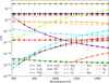 |
Fig. 1 Abundances of various species, ϵ(X)=nX/n〈H〉, obtained with the time-independent PRODIMO models from grid_0 for density n〈H〉= 7.56 × 1013 cm−3 (dots), compared to the corresponding GGchem models (dashed lines). The deviations at the lowest temperatures are due to numerical problems in converging the PRODIMO models. |
4.2 Chemical relaxation timescale
We now analyse the chemical relaxation timescale (τchem) in the disk where the kinetic chemistry approaches thermodynamic equilibrium. This can tell us whether thermodynamic equilibrium can be established on disk-evolutionary timescales. We realise that there can be various definitions for chemical relaxation timescales and explore them here. We define the chemical relaxation timescale in the following two different ways:
 (12)
(12)
 (13)
(13)
where Fi and Di are the total formation and destruction rates, respectively, of species i. τchem, 1 can be computed from the diagonal elements in the chemical Jacobian. The slowest species determines the relaxation timescale. Equation (12) is easy to understand but lacks a proper mathematical foundation. Using perturbation theory and linear algebra, the proper mathematical formulation of the relaxation timescale involves a transformation of the Jacobian into n eigenvectors (the chemical modes) which each relax on individual timescales given by the inverse of the real part of their eigenvalues, λn. The slowest of these modes determines the chemical relaxation timescale, τchem, 2, according to Eq. (13), (see Woitke et al. 2009), with values listed in Table 7. Since a chemical network obeys a number of auxiliary conditions in the form of the conservation of the elements, the major element carriers must not be considered in Eq. (12), and the Nel slowest modes must be discarded in Eq. (13), where Nel is the number of elements.
Figure 2 depicts the evolving abundances of various species in two time-dependent chemical models at 1200 K and 2000 K using a density of 7.65 × 1013 cm−3. We can visually read from this figure that the PRODIMO abundances only approach the GGchem values after ∼108 yr(τchem, 3) in the 1200 K model, but already approach them after ∼0.1 yr in the 2000 K model. These examples show how strongly the chemical relaxation timescale increases with decreasing temperature. While all three timescales at 2000 K are relatively similar, the timescale at 1200 K from the first definition (τchem, 1) is about four orders of magnitude lower than τchem, 2 and the visually determined value from the figure, which are both similar.
Hence, τchem, 1 can be misleading. For example, proton exchange reactions between N2 and N2H+ have high rates, yet these reactions do not contribute to the formation and destruction of the strong N ≡ N bonds. Therefore, studying the chemical relaxation timescale of the chemical modes (eigenvectors of the Jacobian) is more reliable than the first definition. However, even that method does not predict the chemical relaxation timescale fully satisfactorily in all cases, especially when we consider even lower temperatures where the chemical relaxation timescale can easily become greater than the age of the universe. One of the possible explanations is that there are numerical problems when decomposing the chemical Jacobian into its eigenvectors. This is due to the extremely high conditional numbers of the matrix. Thus, from this analysis, we conclude that it is not trivial to reliably evaluate the chemical relaxation timescale that can have a huge range of fast and slow modes.
During this analysis, we find that species such as SiH take extremely long to reach their equilibrium abundances based on a preliminary network. This indicates that this preliminary chemical network is incomplete for silicon-hydrides, as both UMIST 2022 and STAND only include reactions of Si-hydrides with charged species but no neutral-neutral reactions. We therefore added a few reactions from Raghunath et al. (2013) and NIST (Manion et al. 2015), as listed in Table 2, to the CHAITEA chemical network. This leads to a much faster relaxation of the Si-hydride molecules. However, once this problem is solved, the next molecules that present this issue are N-bearing species, which is further discussed in the following section. This might indicate that the network for these species is also not yet complete.
Chemical relaxation timescales obtained with different methods for 1200 K and 2000 K models at n〈H〉=7.5 × 1013 cm−3, using time-dependent (t-dep.) and time-independent (t-indep.) chemistry.
4.3 The N2 formation problem
Figure 2 shows that N-bearing species such as HCN, NH3, and CN are the slowest to attain thermodynamic equilibrium at 1200 K, which happens only after ∼108 years. We analyse here the time-dependent behaviour at various steps for the two temperatures 1200 K and 2000 K. We started our simulations by putting all elements into their highest ionisation state as an initial condition, except for neutral hydrogen, which has an initial abundance of 10−5. The gas recombines within 10−8 yr (i.e. in less than one second) at both temperatures. After about 10−6 yr (∼30 s), neutral molecules form by consuming the neutral atoms via barrier-free, exothermic neutral-neutral and termolecular reactions such as
 (14)
(14)
 (15)
(15)
 (16)
(16)
 (17)
(17)
This phase results in the creation of many simple neutral molecules that all attain similar abundances, as they are all produced by almost equally fast reactions. Most of the atoms are consumed after about 0.1 yr (one month) at 1200 K and about 0.0001 yr (one hour) at 2000 K. At this time, the chemistry slows down substantially. Some parts of the network, such as the hydrocarbon chemistry, have already reached internal detailed balance, but as these parts are only weakly connected to other parts of the network, such as the N- and O-chemistry, the connections have not yet reached equilibrium. Eventually, after about 0.1 yr in the 2000 K model, each molecule has reached thermodynamic equilibrium. However, in the 1200 K model, after 103 yr all molecules have reached thermodynamic equilibrium except for the N-bearing species, which take as long as 108 yr to reach equilibrium. This final phase is characterised by difficulties in forming the thermodynamically favoured N2 from the other overabundant N molecules. All the reactions stated above become extremely inefficient due to the lack of free atoms at 1200 K. The following reaction is found to be most effective in reducing the N-bearing species and forming N ≡ N bonds:
 (18)
(18)
but since both NO and NH2 are not very abundant molecules in thermodynamic equilibrium, this reaction channel takes as long as 108 yr in this example.
This analysis indicates that we may miss some other neutral-neutral reaction pathways to form or destroy N ≡ N bonds, in order to reduce the chemical relaxation timescale. We experimented with adding N2H, NCN, and HNCO to our network, which indeed leads to a slight decrease in the relaxation timescales, but only by a factor of 2−3, and we are unable to solve the general problem this way. One possibility might be to include surface reactions to form N2 on much shorter timescales. At temperatures ⩽ 1100 K, the chemical relaxation timescale derived from Eq. (13) becomes longer than the age of the universe. This issue was also reported by Le Gal et al. (2014). The neutral-neutral reactions forming N2 mentioned by Pineau des Forets et al. (1990) and Hily-Blant et al. (2010) are included in the chemical network but are not found to be dominant.
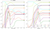 |
Fig. 2 Abundances, ϵ(X)=nX/n〈H〉, of various species (X) as a function of time obtained with Pro DI Mo at 1200 K and 2000 K at a density of n〈H〉 = 7.56 × 1013 cm−3. The large coloured dots represent the abundances in thermodynamic equilibrium obtained with GGchem. |
4.4 Deviations from thermodynamic equilibrium
Figure 3 depicts the deviations from thermodynamic equilibrium at different temperatures and densities when photoprocesses, X-rays, and cosmic rays are switched off (grid_0). We define the deviation as
 (19)
(19)
where ni is the PRODIMO particle density and  is the GGchem particle density. N is the number of species found in both models. To avoid picking up differences between particle densities at extremely low abundances such as 10−80, which PRODIMO does not predict properly, we used a summation weight of
  . In this way, a deviation of one order of magnitude at an abundance of 10−20 is evaluated as as poor as a deviation of 10−4 at unit abundance. The mean deviation, σ, varies across temperature and density. We excluded Mg, Mg+, Fe, Fe+, Na, and Na+in Eq. (19) because the selection of Mg-, Na- and Fe- bearing species is incomplete in PRODIMO, causing large deviations at low temperatures where GGchem predicts these metals to be present in the form of hydroxides such as Mg(OH)2, Fe(OH)2, and (NaOH)2, respectively.
As shown in Fig. 3, the deviations are <1% across all densities and temperatures considered, implying that our new CHAITEA chemical network is capable of relaxing towards thermodynamic equilibrium, as expected. These deviations are caused by small differences in the thermochemical data between PRODIMO and GGchem, and due to the different selections of molecular species.
The species that contributes the most to σ is marked by the white labels in Fig. 3. We do not observe any ions because these models are in thermodynamic equilibrium and the deviations are caused mostly by the abundant neutrals. At the lowest temperatures, there are a few cases where the PRODIMO models do not converge, as indicated by the blank rectangles. The deviations are much larger there, only for numerical reasons. In all the cases where the PRODIMO models converge, the deviations from thermodynamic equilibrium are found to be small (<1%). Hence, we consider our first test to be passed: the CHAITEA network relaxes towards thermodynamic equilibrium down to ∼600 K in the absence of any processes causing deviations from it.
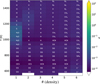 |
Fig. 3 Deviation σ (see Eq. (19)), between particle densities obtained with time-independent PRODIMO (ni) and GGchem |

4.5 Effect of photoreactions
We relaxed condition number (iv) (see Sect. 4.1), leading to grid_photo, and perform a similar analysis to study the effect of photoreactions on thermodynamic equilibrium. As shown in Fig. 4, the maximum deviation, σ, is then of the order of 10−1. The radiative association reactions become relatively more significant at low densities, causing larger differences in the particle densities between GGchem and PRODIMO. The deviations at higher densities are caused by ions such as H3 O+ and H−, at all temperatures. As the ions are more abundant in PRODIMO relative to GGchem, this results in larger deviations from thermodynamic equilibrium.
There is a gradual increase in σ going towards low densities. This is because the photoreactions scale with n〈H〉. Higher temperatures are affected more as the rates of these photoreactions increase with temperature (Planck radiation field). Reactions such as
 (20)
(20)
cause species such as e− and H−to deviate from detailed balance. H3O+ is not in perfect detailed balance due to
 (21)
(21)
which is an auto-generated reaction (see Sect. 3.2).
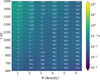 |
Fig. 4 Same as Fig. 3 but from grid_photo which includes photo processes based on a local Planck field Jv = Bv(T), radiative association, and direct recombination reactions. |
4.6 Effect of cosmic rays
In this section, photo rates were again turned off. The deviations, σ, are presented in Fig. 5 for various CRIs at different densities and temperatures. The deviations increase with increasing CRI.
Across all densities and CRIs, σ increases strongly with decreasing temperature. This is because the CRIs are independent of temperature, whereas the neutral-neutral gas-phase reaction rates decrease strongly with temperature because of the activation barriers. A secondary trend is that σ increases for lower densities. This effect is because the CRI scale with n〈H〉, whereas the gas-phase chemical reactions scale with  or
or  .
.
As the CRI increases, the ions are affected first as they are the primary species created by the cosmic rays. Eventually, the neutrals are also affected at all temperatures and densities. High levels of cosmic rays create more reactive radicals such as OH, and CH3, which promote neutral-neutral chemistry. This results in neutrals deviating from thermodynamic equilibrium. For instance, at 1000 K and a density of n〈H〉 = 7.562 × 1013 cm−3, we observe that with increasing CRI, the molecule that causes the largest deviations shifts from He+ to NH3. At a CRI of 1.7 × 10⁻¹⁷ s−1, which is typically used in disk models, σ is of the order of 1 at high temperatures (>1100 K), but as large as 30 at low temperatures; i.e. the abundances in kinetic chemical equilibrium deviate from thermodynamic equilibrium by 30 orders of magnitude on average.
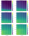 |
Fig. 5 Impact of cosmic-ray ionisation rate on deviations from thermodynamic equilibrium at different densities and temperatures from grid_cr. The adopted values of CRIs are listed at the top of each panel. The x- and y-axes are the same as in Fig. 3. |
4.7 The chemical deviations in a full disk model
In this section, we study the abundances in a 2D disk model around a T Tauri star, and evaluate the differences between the chemical solutions obtained with PRODIMO in kinetic chemical equilibrium and with GGchem in thermodynamic equilibrium. The disk model is outlined in Sect. 3.5 and our choices of stellar, disk shape, dust size and opacity parameters are listed in Table C.1. We excluded ices, PAHs and excited H2* for this comparison, because these species are not included in GGchem. The model has a grid resolution of 200 × 300 and includes UV, cosmic rays and X-ray chemistry. The second disk model, called GGchem, uses GGchem and the densities and gas temperatures calculated in the PRODIMO model.
Figures 6 and 7 show the abundances of various molecules from these models, demonstrating how different these solutions are. As Woitke et al. (2021) discuss, the molecular abundances in thermodynamic equilibrium at low temperatures (T < 500 K) have a binary character: either a molecule is very abundant and is the major carrier of an element or it only attains a trace abundance. This is because at low temperatures the contribution of entropy term is low and the code maximises the binding energy of the molecules. In the case of the elemental abundances considered in this paper, these molecules are H2, H2O, CH4, NH3, H2S, SiH4, Mg(OH)2, Fe(OH)2, and (NaOH)2. All other molecules have extremely low abundances in the GGchem model in the outer disk regions where the temperature is low. Molecules such as CO, CO2, and N2 are only present in the GGchem model in a relatively thin intermittent surface layer where the temperatures are ∼1000 K due to the heating by UV processes. Temperatures exceed 5000 K above this layer, which is too high for molecules to exist in high abundances.
The abundances calculated with chemical kinetics by the PRODIMO model are different (Figs. 6, 7, left column). The cosmic rays constantly create small amounts of ions, atoms, and neutral radicals, that drive all the important gas-phase reactions and prevent the chemistry from relaxing towards thermodynamic equilibrium.
In particular, oxygen is stored in H2 O in thermodynamic equilibrium, whereas it is distributed among H2O, CO2, and CO in kinetic equilibrium. Carbon is locked in CH4 in thermodynamic equilibrium throughout the cold disk, whereas it is found in the form of CO2 and CO in kinetic equilibrium, similarly to in Bergin (2009). The main carrier of N in thermodynamic equilibrium is NH3 in the entire cold disk, but switches to N2 in the warm disk surface. In kinetic chemical equilibrium, N mostly forms N2 with HCN and NH3 in the inner disk (≲0.5 au), as seen in Fig. 7.
Figure 8 shows the average chemical deviation, σ, between the two models as a function of disk radius, r, and height over the midplane, z. The minimum σ is ∼1, indicating that thermodynamic equilibrium likely does not exist in any disk region. The inner midplane regions of the disk, directly behind the inner rim inside about 0.1 au, are closest to thermodynamic equilibrium, because radiation such as cosmic rays is shielded here. As we go either vertically up or radially outwards in the disk, σ becomes larger. These large σ are due to the effect of irradiation by UV, X-rays, and cosmic rays. The outer midplane is affected by cosmic rays whereas UV and X-rays affect the chemistry in warm surface layers and prevent relaxation towards thermodynamic equilibrium. There is, however, the warm molecular intermittent surface layer where σ again reaches values as low as 5. Here, the gas-phase chemical reactions can compete with the cosmic-ray, X-ray, UV-induced chemistry, because temperatures are high enough to overcome the activation energies of the neutral-neutral reactions. However, the chemistry is still not in thermodynamic equilibrium. We also tested another criterion where σ is only affected when  . However, we still observe a similar deviation between the kinetic chemical equilibrium and the thermodynamic equilibrium.
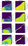 |
Fig. 6 Abundances of selected species in the 2D disk model calculated using chemical kinetics (left) and thermodynamic equilibrium (right). The white contours correspond to the tick values on the colorbars. |
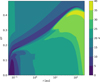 |
Fig. 8 Deviation (σ) between kinetic chemical equilibrium and thermodynamic equilibrium in the 2D disk model. σ = 1 denotes a deviation of one order of magnitude between the PRODIMO and GGchem abundances. |
5 Implications for disk kinetic chemistry
To assess the implications of the above work for kinetic chemical networks, we studied the effect of extending the large DIANA standard network (Kamp et al. 2017) to the new CHAITEA chemical network on the 2D abundances in thermochemical disk models. We investigated this question in two steps; see Table 8. First, we added the reverse reactions based on the same Gibbs free energies as discussed in this paper, and second, we added the STAND reactions which have preference over the UMIST 2022 and DIANA reactions.
In all these models, the same 239 species were selected. We added excited molecular hydrogen  , five charging states of PAHs, and the ices of all neutral species to the list of species in Table 1. Compared to the original large DIANA (Kamp et al. 2017) standard network consisting of 235 species, there was also N2O, N2O+, HNO2+, and N2O#, as we needed N2 O for the Si hydride reactions (Table 2). Following the rules laid out by Kamp et al. (2017) for developing a network, we also added N2O+ and HNO2+. This was our final CHAITEA network. The disk model was the same as in the previous section, see Table C.1. The gas temperature was consistently calculated with the chemistry in each of the following models. UV-photo, X-ray and cosmic rays processes were included.
5.1 Effect of adding the reverse reactions
Table 8 shows that the inclusion of the reverse reactions mostly increases the number of endothermic reactions, as most of these are derived from their exothermic counterparts. It also “auto-cleans” the network by correcting spurious endothermic reactions with zero or extremely low activation energies, which are unrealistic, as discussed in Sect. 3.3.
Our results are presented in Figs. D.1, D.2, and D.3. The left columns in these figures show the model with the large DIANA and UMIST 2022 reactions, whereas the middle column also includes the reverse of these reactions. By comparing the left and middle columns in these figures, we observe that the abundances of most molecules are only slightly affected (for example, H2O). However, certain species show significant differences, particularly atomic H close to the outer midplane, and C2H2, CO, CO2, and N2 close to the inner midplane. For these species, the abundances decrease significantly when reverse reactions are included. Additionally, we observe an increase in N2H+ abundance in several disk regions when reverse reactions are considered.
The relatively high abundance of atomic H in the outer midplane of the DIANA-standard model is an example of artefacts caused by spurious endothermic reactions with zero activation energy. One such reaction is
 (22)
(22)
This reaction was included as one of the additional reactions collected by Kamp et al. (2017), referencing Anicich (1993). However, there was an error in its inclusion; the correct reaction is
 (23)
(23)
The erroneous reaction has a reaction enthalpy of about +6.5 eV. While the correct reaction is also endothermic, with +0.43 eV, it is reported as barrier-free with zero activation energy (see Johnsen 2005 for details). In the outer midplane, where C-, N-, O-, and S-bearing species are locked in their respective ices, H3+ is the most abundant molecular cation, maintaining charge balance with free electrons (Balduin et al. 2023). As a result, H3+ is relatively abundant, as is Ar, which leads the model with the erroneous reaction to produce a significant amount of neutral H in the midplane. However, when reverse reactions are included, the forward rate of this reaction is automatically corrected, as it would be for the correct reaction, and the artefact is eliminated. We identify 45 such spurious reactions in the large DIANA-standard network, and 68 when the STAND reactions are added, demonstrating once again that this is a common issue in astrochemistry (Tinacci et al. 2023).
We identify the following reasons for the increase in N2H+ abundance in various disk regions when reverse reactions are considered. First, the following constructed endothermic formation reactions become significant at very high temperatures (several thousand Kelvin):
 (24)
(24)
 (25)
(25)
Second, one of the dominant N2H+ destruction reactions:
 (26)
(26)
is found to be endothermic (+0.12 eV) but is reported as barrier free. This means that at temperatures as low as 20 K, the rate of this reaction is automatically corrected to very low values, leading to an increase in the N2H+abundance.
The abundance structures of H2O, CO, and NH3 are similar between the two models. The abundance of c−C3H2 has three reservoirs. The innermost reservoir within 0.1 au decreases in abundance when the reverse reactions are taken into account, whereas the reservoir around 1 au increases. A similar trend is observed for CH3 at 1 au. The inner reservoir of HCN is smoother in abundance when including the reverse reactions.
The abundance of C2H2 drops in the inner disk (≲0.1 au) between DIANA-standard and DIANA-standard-rev. The reactions mostly contributing to the formation of C2H2 in DIANA-standard are
 (27)
(27)
 (28)
(28)
These reactions are also reported as dominant by Kanwar et al. (2024b) (grid point 3, fiducial model). However, when reverse reactions are included, each of these major formation reactions is balanced by the reverse of these reactions, thus resulting in no net contribution in the inner region (similar to detailed balance). Subsequently, the destruction of C2H2 by cosmic rays becomes dominant, leading to a decrease in abundance. These changes caused by the addition of reverse reactions can be crucial for the interpretation of JWST observations that can probe these deeper inner disk regions.
5.2 Effect of expanding to the CHAITEA network
When comparing the DIANA-standard-rev model to the CHAITEA model (the middle and right columns of Figs. D.1, D.2, D.3), we observe that many molecular abundances are affected in various ways. This outcome is expected, as we replaced the UMIST 2022 reaction data with the STAND reaction set, leading to significant modifications in most of the important chemical reactions. However, the overall impact is not substantial. For example, the abundances of important species such as H2O, CO, and e− remain largely similar between the two models. In light of the mid-infrared and (sub-)millimetre observations, we discuss below a few species that show large differences in their abundance structures between the DIANA-standard-rev and CHAITEA models in more detail.
Between the two models, there are significant differences in the inner midplane that is probed by JWST. For example, the abundance of CO2 increases within 1 au when using the CHAITEA chemical network. This is due to more formation of CO2 in CHAITEA relative to the DIANA-standard-rev model. The dominant formation reaction in CHAITEA model is
 (29)
(29)
This reaction is barrier free according to the STAND network. However, Frost et al. (1993) and Millar et al. (2024) report an activation barrier of 176 K. We investigated whether incorporating this barrier would alter the CO2 abundance structure, but find no significant changes. As a result, the final CHAITEA network retains the reaction as barrier free, consistent with the STAND network. This can be further revisited in future work. The second notable change is a 2 orders of magnitude decrease in C2H2 abundance in the inner and central midplane when using the CHAITEA network. Kanwar et al. (2024b) also report a reduction in C2H2 abundance in the inner midplane when larger hydrocarbons were included in an extended hydrocarbon chemical network. These larger hydrocarbons are not included in the current network and are beyond the scope of this study. Integrating the two networks could thus lead to substantially lower C2H2 abundances but eventually provide a more accurate abundance structure for mid-infrared observations (Tabone et al. 2023; Arabhavi et al. 2024; Xie et al. 2023; Kanwar et al. 2024a; Schwarz et al. 2024). The change in HCN abundance is more complex. In the DIANA-standard-rev model, the thin, higher-abundance surface layer extends farther radially than in the CHAITEA model (see Fig. D.2). There is less formation of HCN in the latter. The major formation pathway in the surface layer in both the models is
 (30)
(30)
In the DIANA-standard-rev model, this reaction has a very low energy barrier (6.3 · 10−4 K). However, in the CHAITEA model, the reaction has a higher barrier of 2.3 · 103 K, resulting in a decrease in HCN abundance in the surface layer by an order of magnitude. The abundance of some ions such as CH+increases in the surface layers of the outer disk in the CHAITEA model and this may affect the interpretation of the Herschel Space Telescope observations (Thi et al. 2011).
There are also significant differences in the outer disk that may affect the inferences from ALMA observations. For example, the abundance of HCN decreases in the CHAITEA model in the surface layers of the outer disk relative to DIANA-standardrev by at least 1.5 orders of magnitude. This could lead to lower line fluxes at millimetre wavelengths when using the CHAITEA chemical network. Other neutral molecules such as NH3, C2H, CH3, and c−C3H2 also show substantially lower abundances in the outer disk when using the CHAITEA chemical network. C2H plays a key role in determining the carbon budget in the outer disk. The abundance of the key molecular ion N2H+ on the other hand increases in the outer disk when using the CHAITEA chemical network. Qi et al. (2015) and, van ’t Hoff et al. (2017) used N2H+to infer the location of the CO iceline in the disk as it is difficult to observe directly. There is also a decrease in the abundances of CH3 and c-C3H2 in the inner disk by 2−3 orders of magnitude in the CHAITEA model compared to DIANA-standard-rev. This can help to interpret JWST (Arabhavi et al. 2024; Kanwar et al. 2024a) and ALMA (Qi et al. 2013; Bergin et al. 2016) observations better.
6 Summary and conclusions
We merged the STAND chemical network developed for planetary and exoplanetary atmospheres (Rimmer & Helling 2016, 2019), which includes pressure-dependent termolecular and reverse reactions based on Gibbs free energy data, with the UMIST 2022 chemical network and our large DIANA standard chemical network developed for disks (Kamp et al. 2017), which was later updated in Kanwar et al. (2024b). A cornerstone in developing the new network was compiling a comprehensive set of Gibbs free energy data from various sources. For some molecules, data had to be estimated using ionisation potentials and proton affinities to ensure all gas-phase reactions could be reversed. This new, integrated chemical network is named CHAITEA.
We then studied under what conditions thermodynamic equilibrium can be established in planet-forming disks. Finally, we explored how the chemical composition of the disk changed when we used the new CHAITEA chemical network instead of the large DIANA standard network. We used a 2D T Tauri disk model for this investigation, including UV, X-ray, and cosmic-ray chemistry:
In the absence of any UV, X-ray or cosmic-ray irradiation, we verify that the new CHAITEA network converges towards thermodynamic equilibrium by benchmarking it against the chemical equilibrium code GGchem (Woitke et al. 2018);
However, at a gas density of 7.56 × 1013 cm−3 (∼10 dyn/cm2), the chemical relaxation timescale τchem, 3, towards thermodynamic equilibrium can be as short as a month at 2000 K, which increases to ∼108 yr at 1200 K, and exceeds the age of the universe at 1100 K;
The chemical relaxation proceeds simultaneously via fast and slow chemical modes with characteristic timescales that differ by many tens of orders of magnitude. We find that one of the slowest modes is the production of N2 from other N-bearing molecules after the neutral atoms are consumed;
The inclusion of radiative association, direct recombination reactions (considered non-reversible), and photo rates based on a local Planck radiation field, Jv = Bv(T), causes deviations from thermodynamic equilibrium by 2−20% across all densities and temperatures studied;
The inclusion of cosmic rays leads to significant deviations from thermodynamic equilibrium, initially affecting the charged molecules and eventually impacting the abundant neutral species. At low temperatures (T ≲ 750 K), even a tiny CRI of 10−40 s−1 alters the neutral chemistry. At the standard CRI of 1.7 × 10⁻¹⁷ s−1, below ∼1200 K, deviations from thermodynamic equilibrium can exceed 10−30 orders of magnitude;
In a 2D disk model, no region is found to be in thermodynamic equilibrium. We find that a small, warm, dense region in the midplane directly behind the inner rim (r ≲ 0.1 au), where the cosmic rays are mostly shielded, is closest to thermodynamic equilibrium, with σ ∼ 1. There is a warm intermittent molecular layer where σ ∼5. In all other regions σ is much larger.
In kinetic equilibrium, nitrogen is primarily stored in N2, carbon in CO and CO2, and oxygen in H2 O and CO, whereas the thermodynamically favoured molecules at low temperatures are NH3 for nitrogen, CH4 for carbon, and H2 O for oxygen;
When using the CHAITEA chemical network, the change in the abundances of species such as CO, H2O and free electrons is not major (an order of magnitude). The abundance of species such as C2H2, HCN and CH4 decreases in the inner midplane, while the abundance of CO2 increases within 1 au. Some molecular cations such as N2H+and CH+ attain larger abundances in the intermittent warm molecular layer and in the outer disk regions. The reasons for these differences are complex. Differences in the rate coefficients of the leading reactions can have profound effects on the resulting abundances. Defining reaction pairs based on Gibbs free energy allows for the identification and automatic correction of spurious endothermic reactions reported with zero or minimal activation energies, which are chemically implausible. Such reactions can significantly impact the chemistry of the outer disk.
The techniques implemented in this work, and the new chemical network developed, can be used to interpret both the (sub-) millimetre molecular lines observable with ALMA and the midinfrared observations with JWST. The latter probes the inner, dense, and warm regions where this network is more complete. The CHAITEA chemical network can also be used to quantify the significance of the termolecular and reverse reactions using the observations.
Acknowledgements
This project has received funding from the European Union’s Horizon 2020 research and innovation programme under the Marie SklodowskaCurie grant agreement No. 860470. We thank the anonymous referee for their constructive comments. We acknowledge discussions with W.F. Thi. J.K. acknowledges productive discussions with Till Kaeufer, Nidhi Bangera, David Lewis, and Ashwani Rajan.
Appendix A Derivation of the law of mass action
We assume a mixture of ideal gases with partial pressures pi = NiRT/V, where Ni are the mol numbers of the gas species i, V is the common volume, and R [J/K/mol] is the ideal gas constant. P = ∑ipi is the total gas pressure. (T⊖, p⊖) denotes a thermodynamical reference state at room temperature T⊖ = 298 K and at standard pressure p⊖ = 1 bar, to which some of the thermodynamic quantities refer to. The thermodynamic description of such mixtures, see Atkin & de Paula (2006), is
 (A.1)
(A.1)
 (A.2)
(A.2)
 (A.3)
(A.3)
 (A.4)
(A.4)
where G is the system Gibbs free energy, U the internal energy, and S the entropy. The small symbols refer to the molar properties of the pure gases  is the internal energy in the standard state (T⊖, p⊖), cV, i the heat capacity, and
  is the entropy in the standard state (T⊖, p⊖). si(T, p⊖) is the entropy of the pure gas i at temperature T and standard pressure p⊖. The terms in the integrals in Eq. (A.4) can be derived from the first law of thermodynamics in the form dU = −PdV + TdS for processes of an ideal gas at constant temperature or pressure. The term R ln (pi/p⊖) is the mixing entropy. Altogether, the system Gibbs free energy is

where gi(T, p⊖) is the molar Gibbs free energy of the pure gas i at temperature T and standard pressure p⊖.
Next, we consider a hypothetical chemical reaction N2 + 3 H2 → 2 NH3, where k = 3, {1 → N2, 2 → H2, 3 → NH3} and stoichiometric coefficients {v1 = −1, v2 = −3, v3 = + 2}. We also consider a small number of mols of such reactions Δ to take place at constant temperature and pressure. The principle of minimisation of the system Gibbs free energy in this case requires that
 (A.5)
(A.5)
in the thermodynamical equilibrium state that is characterised by the mol numbers  . From Eq. (A.5) it follows that
 (A.6)
(A.6)
for any small Δ. The Gibbs free energy data for the pure gases i can be found in various thermochemical databases, here we use Burcat & Ruscic (2005). These data are given as the Gibbs free energy of formation  (T)[J/mol] of a molecule from the standard states of the elements at room temperature. Since any chemical reaction obeys the principle of element conservation, these constants cancel in Eq. (A.6), so we can write this equation also as
 (A.7)
(A.7)
Introducing the reaction Gibbs free energy as
 (A.8)
(A.8)
we find the law of mass action
 (A.9)
(A.9)
Equation (A.9) is valid for all hypothetical chemical reactions in thermodynamical equilibrium, even if they cannot proceed kinetically. We note that ΔG = 0 in thermodynamical equilibrium, whereas ΔRG⊖ ≠ 0 because of the mixing entropy. In the main text in Sect. 2.2 we consider the reaction A + B → C + D + E, where k = 5 and {v1 = −1, v2 = −1, v3 = + 1, v4 = + 1, v5 = + 1}.
Appendix B Thermochemical data of missing species in Burcat format
Table B.1 summarises our efforts to collect, convert, estimate or construct the thermochemical in Burcat format (NASA 7-polynomials) of those species missing in Burcat & Ruscic (2005).
Additional thermochemical data not included in Burcat & Ruscic (2005). ΔfH⊖(0 K) is given in kJ/mol.
Appendix C Disk model parameters
We provide the list of input parameters used to model the disk in Table C.1.
Appendix D Abundances of various species
Figures D.1, D.2 and D.3 show the abundances of various species discussed in Sect. 5. These abundances are calculated using different chemical networks and rate databases that are outlined in Table 8.
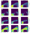 |
Fig. D.1 The abundances of various species in the three models calculated using different chemical networks and rate databases outlined in Table 8. The white dashed contours correspond to the tick values on the colourbar. |
References
- Anicich, V. G., 1993, J. Phys. Chem. Ref. Data, 22, 1469 [NASA ADS] [CrossRef] [Google Scholar]
- Arabhavi, A. M., Kamp, I., Henning, T., et al. 2024, Science, 384, 1086 [NASA ADS] [CrossRef] [Google Scholar]
- Aresu, G., Kamp, I., Meijerink, R., et al. 2011, A&A, 526, A163 [NASA ADS] [CrossRef] [EDP Sciences] [Google Scholar]
- Arrhenius, S., 1889, Zeitschrift für Physikalische Chemie, 4U, 96 [Google Scholar]
- Atkin, P., & de Paula, J., 2006, Atkins’ Physical Chemistry, 8th edn. (Oxford University Press) [Google Scholar]
- Balduin, T., Woitke, P., Jørgensen, U. G., Thi, W. F., & Narita, Y., 2023, A&A, 678, A192 [NASA ADS] [CrossRef] [EDP Sciences] [Google Scholar]
- Barklem, P. S., & Collet, R., 2016, A&A, 588, A96 [NASA ADS] [CrossRef] [EDP Sciences] [Google Scholar]
- Barth, P., Helling, C., Stüeken, E. E., et al. 2021, MNRAS, 502, 6201 [Google Scholar]
- Bergin, E. A., 2009, arXiv e-prints [arXiv:0908.3708] [Google Scholar]
- Bergin, E. A., Du, F., Cleeves, L. I., et al. 2016, ApJ, 831, 101 [Google Scholar]
- Blumenthal, S. D., Mandell, A. M., Hébrard, E., et al. 2018, ApJ, 853, 138 [Google Scholar]
- Burcat, A., & Ruscic, B., 2005, Third millenium ideal gas and condensed phase thermochemical database for combustion (with update from active thermochemical tables), Tech. Rep. (Argonne National Laboratory) [CrossRef] [Google Scholar]
- Carleo, I., Giacobbe, P., Guilluy, G., et al. 2022, AJ, 164, 101 [NASA ADS] [CrossRef] [Google Scholar]
- Chase, Jr., M. 1998, Journal of Physical and Chemical Reference Data, Monograph 9 [Google Scholar]
- Cooper, C. S., & Showman, A. P., 2006, ApJ, 649, 1048 [CrossRef] [Google Scholar]
- Dick, J., 2019, Front. Earth Sci., 7, 668 [Google Scholar]
- Fortney, J. J., Cooper, C. S., Showman, A. P., Marley, M. S., & Freedman, R. S., 2006, ApJ, 652, 746 [CrossRef] [Google Scholar]
- Frost, M. J., Paul, S., & Smith, I. W. M., 1993, J. Phys. Chem., 97, 12254 [Google Scholar]
- Guilluy, G., Giacobbe, P., Carleo, I., et al. 2022, A&A, 665, A104 [NASA ADS] [CrossRef] [EDP Sciences] [Google Scholar]
- Heays, A. N., Bosman, A. D., & van Dishoeck, E. F., 2017, A&A, 602, A105 [NASA ADS] [CrossRef] [EDP Sciences] [Google Scholar]
- Hily-Blant, P., Walmsley, M., Pineau Des Forêts, G., & Flower, D., 2010, A&A, 513, A41 [NASA ADS] [CrossRef] [EDP Sciences] [Google Scholar]
- Johnsen, R., 2005, J. Phys.: Conf. Ser., 4, 83 [Google Scholar]
- Kamp, I., Thi, W. F., Woitke, P., et al. 2017, A&A, 607, A41 [NASA ADS] [CrossRef] [EDP Sciences] [Google Scholar]
- Kanwar, J., Kamp, I., Jang, H., et al. 2024a, A&A, 689, A231 [NASA ADS] [CrossRef] [EDP Sciences] [Google Scholar]
- Kanwar, J., Kamp, I., Woitke, P., et al. 2024b, A&A, 681, A22 [NASA ADS] [CrossRef] [EDP Sciences] [Google Scholar]
- Le Gal, R., Hily-Blant, P., Faure, A., et al. 2014, A&A, 562, A83 [NASA ADS] [CrossRef] [EDP Sciences] [Google Scholar]
- Lindemann, F. A., Arrhenius, S., Langmuir, I., et al. 1922, Trans. Faraday Soc., 17, 598 [Google Scholar]
- Lodders, K., 2003, ApJ, 591, 1220 [Google Scholar]
- Lodders, K., & Fegley, B., 2002, Icarus, 155, 393 [Google Scholar]
- Manion, J. A., Huie, R. E., Levin, R. D., et al. 2015, NIST Chemical Kinetics Database, NIST Standard Reference Database 17, Version 7.0 (Web Version), Release 1.6.8, Data version 2015.09 [Google Scholar]
- Marley, M. S., & Robinson, T. D., 2015, ARA&A, 53, 279 [Google Scholar]
- Millar, T. J., Farquhar, P. R. A., & Willacy, K., 1997, A&AS, 121, 139 [NASA ADS] [CrossRef] [EDP Sciences] [Google Scholar]
- Millar, T. J., Walsh, C., Van de Sande, M., & Markwick, A. J., 2024, A&A, 682, A109 [NASA ADS] [CrossRef] [EDP Sciences] [Google Scholar]
- Molaverdikhani, K., Helling, C., Lew, B. W. P., et al. 2020, A&A, 635, A31 [NASA ADS] [CrossRef] [EDP Sciences] [Google Scholar]
- Moses, J. I., 2014, Philos. Trans. Roy. Soc. Lond. Ser. A, 372, 20130073 [Google Scholar]
- Moses, J. I., Visscher, C., Fortney, J. J., et al. 2011, ApJ, 737, 15 [Google Scholar]
- Padovani, M., Galli, D., & Glassgold, A. E., 2009, A&A, 501, 619 [NASA ADS] [CrossRef] [EDP Sciences] [Google Scholar]
- Padovani, M., Galli, D., & Glassgold, A. E., 2013, A&A, 549, C3 [NASA ADS] [CrossRef] [EDP Sciences] [Google Scholar]
- Pineau des Forets, G., Roueff, E., & Flower, D. R. 1990, MNRAS, 244, 668 [Google Scholar]
- Qi, C., Öberg, K. I., Wilner, D. J., & Rosenfeld, K. A., 2013, ApJ, 765, L14 [NASA ADS] [CrossRef] [Google Scholar]
- Qi, C., Öberg, K. I., Andrews, S. M., et al. 2015, ApJ, 813, 128 [Google Scholar]
- Rab, C., Güdel, M., Padovani, M., et al. 2017, A&A, 603, A96 [NASA ADS] [CrossRef] [EDP Sciences] [Google Scholar]
- Raghunath, P., Lee, Y.-M., Wu, S.-Y., Wu, J.-S., & Lin, M.-C. 2013, Int. J. Quant. Chem., 113, 1735 [Google Scholar]
- Rimmer, P. B., & Helling, C., 2016, ApJS, 224, 9 [NASA ADS] [CrossRef] [Google Scholar]
- Rimmer, P. B., & Helling, C., 2019, ApJS, 245, 20 [NASA ADS] [CrossRef] [Google Scholar]
- Riols, A., & Lesur, G., 2018, A&A, 617, A117 [NASA ADS] [CrossRef] [EDP Sciences] [Google Scholar]
- Schwarz, K. R., Henning, T., Christiaens, V., et al. 2024, ApJ, 962, 8 [NASA ADS] [CrossRef] [Google Scholar]
- Tabone, B., Bettoni, G., van Dishoeck, E. F., et al. 2023, Nat. Astron. [arXiv:2304.05954] [Google Scholar]
- Thi, W. F., Ménard, F., Meeus, G., et al. 2011, A&A, 530, L2 [NASA ADS] [CrossRef] [EDP Sciences] [Google Scholar]
- Tinacci, L., Ferrada-Chamorro, S., Ceccarelli, C., et al. 2023, ApJS, 266, 38 [NASA ADS] [CrossRef] [Google Scholar]
- Troe, J., & Gesell, B. B., 1983, Berichte der Bunsengesellschaft für physikalische Chemie, 87, 161 [Google Scholar]
- Tsai, S.-M., Lee, E. K. H., Powell, D., et al. 2023, Nature, 617, 483 [CrossRef] [Google Scholar]
- van Dishoeck, E. F., Jonkheid, B., & van Hemert, M. C., 2006, Faraday Discuss., 133, 231 [Google Scholar]
- van ’t Hoff, M. L. R., Walsh, C., Kama, M., Facchini, S., & van Dishoeck, E. F. 2017, A&A, 599, A101 [CrossRef] [EDP Sciences] [Google Scholar]
- Venot, O., Agúndez, M., Selsis, F., Tessenyi, M., & Iro, N., 2014, A&A, 562, A51 [NASA ADS] [CrossRef] [EDP Sciences] [Google Scholar]
- Woitke, P., 2015, in European Physical Journal Web of Conferences, 102, 00011 [Google Scholar]
- Woitke, P., Kamp, I., & Thi, W. F., 2009, A&A, 501, 383 [NASA ADS] [CrossRef] [EDP Sciences] [Google Scholar]
- Woitke, P., Min, M., Pinte, C., et al. 2016, A&A, 586, A103 [NASA ADS] [CrossRef] [EDP Sciences] [Google Scholar]
- Woitke, P., Helling, C., Hunter, G. H., et al. 2018, A&A, 614, A1 [NASA ADS] [CrossRef] [EDP Sciences] [Google Scholar]
- Woitke, P., Herbort, O., Helling, C., et al. 2021, A&A, 646, A43 [NASA ADS] [CrossRef] [EDP Sciences] [Google Scholar]
- Woitke, P., Thi, W. F., Arabhavi, A. M., et al. 2024, A&A, 683, A219 [NASA ADS] [CrossRef] [EDP Sciences] [Google Scholar]
- Xie, C., Pascucci, I., Long, F., et al. 2023, ApJ, 959, L25 [NASA ADS] [CrossRef] [Google Scholar]
- Zahnle, K., Marley, M. S., & Fortney, J. J., 2009a, arXiv e-prints [arXiv:0911.0728] [Google Scholar]
- Zahnle, K., Marley, M. S., Freedman, R. S., Lodders, K., & Fortney, J. J. 2009b, ApJ, 701, L20 [Google Scholar]
All Tables
Critical densities beyond which termolecular reactions and their high-pressure limits become important.
Formation and destruction of C2H2 in kinetic chemical equilibrium at T = 1200 K and n〈H〉=7.56 × 1013 cm−3.
Chemical relaxation timescales obtained with different methods for 1200 K and 2000 K models at n〈H〉=7.5 × 1013 cm−3, using time-dependent (t-dep.) and time-independent (t-indep.) chemistry.
Additional thermochemical data not included in Burcat & Ruscic (2005). ΔfH⊖(0 K) is given in kJ/mol.
All Figures
|
Fig. 1 Abundances of various species, ϵ(X)=nX/n〈H〉, obtained with the time-independent PRODIMO models from grid_0 for density n〈H〉= 7.56 × 1013 cm−3 (dots), compared to the corresponding GGchem models (dashed lines). The deviations at the lowest temperatures are due to numerical problems in converging the PRODIMO models. |
| In the text | |
|
Fig. 2 Abundances, ϵ(X)=nX/n〈H〉, of various species (X) as a function of time obtained with Pro DI Mo at 1200 K and 2000 K at a density of n〈H〉 = 7.56 × 1013 cm−3. The large coloured dots represent the abundances in thermodynamic equilibrium obtained with GGchem. |
| In the text | |
|
Fig. 3 Deviation σ (see Eq. (19)), between particle densities obtained with time-independent PRODIMO (ni) and GGchem |
| In the text | |
|
Fig. 4 Same as Fig. 3 but from grid_photo which includes photo processes based on a local Planck field Jv = Bv(T), radiative association, and direct recombination reactions. |
| In the text | |
|
Fig. 5 Impact of cosmic-ray ionisation rate on deviations from thermodynamic equilibrium at different densities and temperatures from grid_cr. The adopted values of CRIs are listed at the top of each panel. The x- and y-axes are the same as in Fig. 3. |
| In the text | |
|
Fig. 6 Abundances of selected species in the 2D disk model calculated using chemical kinetics (left) and thermodynamic equilibrium (right). The white contours correspond to the tick values on the colorbars. |
| In the text | |
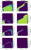 |
Fig. 7 Continued from Fig. 6. We note the different scaling of the GGchem results for HCN and C2H2. |
| In the text | |
|
Fig. 8 Deviation (σ) between kinetic chemical equilibrium and thermodynamic equilibrium in the 2D disk model. σ = 1 denotes a deviation of one order of magnitude between the PRODIMO and GGchem abundances. |
| In the text | |
|
Fig. D.1 The abundances of various species in the three models calculated using different chemical networks and rate databases outlined in Table 8. The white dashed contours correspond to the tick values on the colourbar. |
| In the text | |
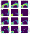 |
Fig. D.2 Continued from Fig. D.1 |
| In the text | |
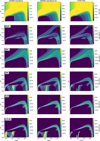 |
Fig. D.3 Continued from Fig. D.2 |
| In the text | |
Current usage metrics show cumulative count of Article Views (full-text article views including HTML views, PDF and ePub downloads, according to the available data) and Abstracts Views on Vision4Press platform.
Data correspond to usage on the plateform after 2015. The current usage metrics is available 48-96 hours after online publication and is updated daily on week days.
Initial download of the metrics may take a while.