| Issue |
A&A
Volume 675, July 2023
|
|
|---|---|---|
| Article Number | A35 | |
| Number of page(s) | 15 | |
| Section | Planets and planetary systems | |
| DOI | https://doi.org/10.1051/0004-6361/202245143 | |
| Published online | 30 June 2023 | |
The β Pictoris system: Setting constraints on the planet and the disk structures at mid-IR wavelengths with NEAR★
1
LESIA, Observatoire de Paris, Univ. Paris-Cité, Univ. PSL, CNRS, Sorbonne Univ.,
5 pl. Jules Janssen,
92195
Meudon, France
e-mail: This email address is being protected from spambots. You need JavaScript enabled to view it.
2
National Astronomical Observatory of Japan, Subaru Telescope,
650 North A’ohōkū Place,
Hilo, HI
96720, USA
3
Department of Physics and Astronomy, University College
London Gower Street,
WC1E 6BT
London, UK
4
Université Paris-Saclay, Université Paris Cité CEA, CNRS, AIM,
91191
Gif-sur-Yvette, France
5
Instituto de Astrofísica de Andalucía, CSIC,
Glorieta de la Astronomía s/n,
18008
Granada, Spain
6
Université Grenoble Alpes, CNRS, IPAG,
38000
Grenoble, France
7
IRAP, Université de Toulouse, CNRS, UPS, CNES,
Toulouse, France
8
Leiden Observatory, Leiden University,
PO Box 9513,
2300 RA
Leiden, The Netherlands
9
STAR Institute, Université de Liège,
Allée du Six Août 19c,
4000
Liège, Belgium
10
Université de Lyon, Université Lyon1, ENS de Lyon, CNRS, Centre de Recherche Astrophysique de Lyon UMR 5574,
69230
Saint-Genis-Laval, France
11
Max Planck Institut für Astronomie,
Königstuhl 17,
69117
Heidelberg, Germany
12
Laboratoire J.-L. Lagrange, Université Côte d'Azur, CNRS, Observatoire de la Côte d’Azur,
06304
Nice, France
13
Centro de Astrobiología (CAB), CSIC-INTA, ESAC Campus,
Camino bajo del Castillo s/n,
28692
Villanueva de la Cañada, Madrid, Spain
14
Astrobiology Center of NINS,
2-21-1 Osawa, Mitaka,
Tokyo
181-8588, Japan
15
Steward Observatory, University of Arizona,
Tucson, AZ
85721, USA
16
College of Optical Sciences, University of Arizona,
Tucson, AZ
85721, USA
17
Aix-Marseille Univ., CNRS, CNES, LAM,
Marseille, France
18
Lund Observatory, Department of Astronomy and Theoretical Physics, Lund University,
Box 43,
221 00
Lund, Sweden
19
European Southern Observatory,
Karl-Schwarzschild-Str. 2,
85748
Garching, Germany
Received:
5
October
2022
Accepted:
8
March
2023
Abstract
Context. β Pictoris is a young nearby system hosting a well-resolved edge-on debris disk, along with at least two exoplanets. It offers key opportunities for carrying out detailed studies of the evolution of young planetary systems and their shaping soon after the end of the planetary formation phase.
Aims. We analyzed high-contrast coronagraphic images of this system, obtained in the mid-infrared, taking advantage of the NEAR experiment using the VLT/VISIR instrument, which provides access to adaptive optics, as well as phase coronagraphy. The goal of our analysis is to investigate both the detection of the planet β Pictoris b and of the disk features at mid-IR wavelengths. In addition, by combining several epochs of observation, we expect to constrain the position of the known clumps and improve our knowledge on the dynamics of the disk.
Methods. We observed the β Pictoris system over two nights in December 2019 in the 10–12.5 µm coronagraphic filter. To evaluate the planet b flux contribution, we extracted the photometry at the expected position of the planet and compared it to the flux published in the literature. In addition, we used previous data from T-ReCS and VISIR in the mid-IR, updating the star's distance, to study the evolution of the position of the southwest clump that was initially observed in the planetary disk back in 2003.
Results. While we did not detect the planet b, we were able to put constraints on the presence of circumplanetary material, ruling out the equivalent of a Saturn-like planetary ring around the planet. The disk presents several noticeable structures, including the known southwest clump. Using a 16-yr baseline, sampled with five epochs of observations, we were able to examine the evolution of the clump. We found that the clump orbits in a Keplerian motion with a semi-major axis of 56.1−0.3+0.4 au. In addition to the known clump, the images clearly show the presence of a second clump on the northeast side of the disk as well as possibly fainter and closer structures that are yet to be confirmed. Furthermore, we found correlations between the CO clumps detected with ALMA and the northeastern and southwestern clumps in the mid-IR images.
Conclusions. If the circumplanetary material were located at the Roche radius, the maximum amount of dust determined from the flux upper limit around β Pictoris b would correspond to the mass of an asteroid of 5 km in diameter. Finally, the Keplerian motion of the southwestern clump is possibly indicative of a yet-to-be detected planet or signals the presence of a vortex.
Key words: planet-disk interactions / instrumentation: high angular resolution / methods: observational / instrumentation: adaptive optics
Based on data collected at the European Southern Observatory under programs 60.A-9107(K), 095.C-0425(A), and 60.A-9234(A).
© The Authors 2023
 Open Access article, published by EDP Sciences, under the terms of the Creative Commons Attribution License (https://creativecommons.org/licenses/by/4.0), which permits unrestricted use, distribution, and reproduction in any medium, provided the original work is properly cited.
This article is published in open access under the Subscribe to Open model. This email address is being protected from spambots. You need JavaScript enabled to view it. to support open access publication.
1 Introduction
Exploring the diversity of planetary systems requires a broad spectral range tuned for detecting various components in these environments: gas, dust, planetesimals, and planets. The past two decades have seen the development of extreme adaptive optics (AO) on monolithic telescopes, a technology that allows for high angular resolution and high contrast imaging to be performed at both visible and near-infrared (NIR) wavelengths. Instruments such as the Spectro-Polarimetric High-contrast Exo-planet REsearch (SPHERE; Beuzit et al. 2019) are sensitive to the thermal emission of young giant planets, as well as the scattered light from dust particles. At the same time, the Atacama Large Millimeter/submillimeter Array (ALMA) has revolutionized observations of the thermal radiation emitted from gas components and millimeter dust grains in both debris disks and gas-rich protoplanetary disks (e.g., ALMA Partnership 2015). The intermediate spectral range, the mid-IR, has received much less attention thus far, primarily because of the high thermal background contamination in ground-based observations. However, this paradigm is about to change thanks to the James Webb Space Telescope and its Mid-Infrared Instrument (MIRI; Rieke et al. 2015; Wright et al. 2015 and references there-in), as well as (later in the decade) the upcoming Mid-infrared ELT Imager and Spectrograph (METIS; Brandl et al. 2018).
In the meantime, the New Earths in the α Centauri Region project (NEAR; Kasper et al. 2019) was installed at the VLT to perform a deep observing campaign of α Centauri (Wagner et al. 2021) and (as part of the Breakthrough Initiatives Foundation) offered an upgrade of the existing VLT spectrometer and imager for the mid-infrared instrument (VISIR; Lagage et al. 2004), which operates in the L, N, and Q bands. Then, VISIR was moved to UT4 for a period of time to benefit from the Adaptive Optics Facility on the secondary mirror (Arsenault et al. 2017) and an annular groove phase mask (AGPM) coronagraph (Mawet et al. 2005; Delacroix et al. 2012) was installed, operating in a single broad filter covering from 10 µm to 12.5 µm, with the filter centered at 11.25 µm (Maire et al. 2020). We took advantage of the NEAR Science Demonstration program to observe the β Pictoris system.
β Pictoris is a young  Myr; Miret-Roig et al. 2020) and bright main sequence pulsating star. Since the discovery of its debris disk by Smith & Terrile (1984), this system has been extensively observed to search for signs of planets. First indirect clues of a planet were brought by the detection of star-grazing comets falling onto the star (Lagrange-Henri et al. 1988) and of a warp in the disk attributed to the gravitational interaction between an unseen massive body (planet, brown dwarf, etc.) on an inclined orbit and the planetesimals in the disk (Mouillet et al. 1997). According to surface brightness measurements, the plan-etesimals are distributed within ~ 120 au, while the inner part inside ~80 au is warped (Augereau et al. 2001). In scattered light, small dust particles, blown by the stellar radiation pressure, have been observed at even larger projected separations (Janson et al. 2021).
Years later, observations with AO of the NaCo instrument at the VLT led to the detection of the thermal emission from the giant planet β Pictoris b (Lagrange et al. 2009, 2010). Finally, in 2019, a second planet β Pictoris c, was identified via radial velocity as a result of nearly 10 yr of monitoring the host-star with the High Accuracy Radial velocity Planet Searcher (HARPS) instrument (Lagrange et al. 2019). This planet c was then confirmed with long-baseline optical interferometry (Nowak et al. 2020; Lagrange et al. 2020).
The β Pictoris system is certainly unique to probe the mechanisms of planetary formation. A large fraction of the previous studies focused on the characterization of the disk and, in particular, on the possible interaction between planets with the dust and gas components by identifying the different features in various spectral regimes and spatial scales. In that respect, Apai et al. (2015) provided a comprehensive analysis of the system by using data obtained in various spectral bands: optical, near IR, mid-IR, and sub-millimeter. Asymmetries, especially between the northeast and the southwest arms of the edge-on disk, are reported at all wavelengths both in scattered light, tracing the submicron-size grains, and in emission, through the analysis of micron-size and sub-millimeter-size grains. A striking feature in the mid-IR is the clump identified in the southwest by Telesco et al. (2005), located at a projected separation of 52 au. The clump was confirmed by Pantin et al. (2005), and recovered by Li et al. (2012) with a small offset, which was interpreted as orbital Keplerian motion. In addition, this asymmetric feature appears at ~10 µm and fades away at ~20 µm, indicative that its flux is dependent on either temperature, grain size, composition, or a combination of these three effects. Telesco et al. (2005) argued that this clump could be the result of either collisions among planetesi-mals trapped in resonance, or the dismantling of a more massive object. Finally, Okamoto et al. (2004) reported amorphous silicates peaks at about 6, 16, and 30 au of radial distance from the central star, and a recent study revisited Spitzer data identifying various rings based on amorphous silicates peaks (Lu et al. 2022).
In addition to the dust clumps observed in the mid-IR, ALMA identified the presence of spatially extended features from both a CO (Dent et al. 2014; Matrà et al. 2017) and neutral carbon (Cataldi et al. 2018) gas. The CO clump can be readily explained because CO would be mainly produced in the brightest dust clump and is overabundant there. Indeed, CO would not have time to spread around its orbit and become axisym-metric because the photodissociation timescale is much smaller than the orbital timescale and CO cannot complete a full orbit. Thus, when observed edge-on, it still looks like a clump similar to the dust clump. With regard to carbon, a clump is much more complicated to explain with current models as carbon gas is expected to survive over Myr timescales (Kral et al. 2016) and to quickly become symmetrical in azimuth because of collisions with ambient gas (even if it were produced in an asymmetric clump initially).
In this work, we analyze, for the very first time, the mid-IR images of β Pictoris obtained using adaptive optics technology, which enables us to reach an unprecedented angular resolution and contrast at this wavelength for this emblematic system. Furthermore, we revisit former VISIR data to perform a multi-epoch comparison. As a result, we provide important constraints on the planet and the disk structures.
The paper is organized as follows: Sect. 2 presents the context of the observations, as well as the data reduction and post-processing. We discuss the non-detection of the planet b in Sect. 3 and we put some constraints on the presence of dust material around the planet in Sect. 3.3. In Sect. 4, we analyze the disk structures and measure the variations of the southwest clump position to better constrain its orbital radius in the system, which is described in Sect. 5. Section 6 covers the other clumps detected in the disk. Finally, we discuss the implications of these observations in Sect. 7 and we present our conclusions in Sect. 8.
2 Observations and data reduction
2.1 VISIR NEAR science demonstration data
2.1.1 Project description
The VLT mid-infrared imager, VISIR, has been modified in the framework of the NEAR project (Kasper et al. 2019) for an observation campaign of the α Centauri system aiming at detecting terrestrial planets. NEAR is supported by ESO and the Breakthrough Initiatives Foundation. The project was designed to push VISIR N-band performances to their limit, in terms of sensitivity and contrast. To that aim, VISIR was equipped with phase mask vortex coronagraphs (AGPM; Mawet et al. 2005; Delacroix et al. 2012) optimized for the 10–12.5 µm band. The control of the centering of the star into the coronagraph was performed with the quadrant analysis of coronagraphic images for tip-tilt sensing estimator (QACITS; Huby et al. 2015; Maire et al. 2020). Also, NEAR has been coupled to a visible wavefront sensor that controls the deformable secondary mirror (DSM) of the adaptive optics facility (UT4), allowing access to extreme adaptive optics regime and reaching Strehl ratios higher than 90% at 12 µm.
2.1.2 Observing setup
β Pictoris was observed with NEAR on the 12th and the 15th of December 2019 (program ID 60.A.9107 (K), P.I. NEAR team). Coupling NEAR with the DSM of the VLT allowed for the use of AO without increasing the number of warm optics that would add to the thermal background. The NEAR spectral filter transmits light from 10 to 12.5 µm and the full width at half maximum (FWHM) is ~ 0.28″, or ~6 pixels. The Cassegrain instrument was fixed in pupil-stabilized mode during the observations. To suppress the large thermal background, a chopping frequency of 8.33 Hz has been adopted and a chop throw of 4.5″. This relatively high frequency allowed to significantly decrease the low-frequency noise excess of the Aquarius type detector (Ives et al. 2014) and reach background limited sensitivity performances. To compensate for the difference in optical path induced by the chopping, the nodding was performed by slightly slewing the telescope every minute. The subtraction of the chopping yielded to have two images of the star taken at different positions: one coronagraphic and the other an off-axis, non-coronagraphic image. As a result, there are two negative images of the star on the side of the central coronagraphic image.
The detector integration time was set to 6 ms to avoid saturation in the background. Ten frames were acquired and stacked in each DSM chopper position, out of which the first two were discarded to suppress any point spread function (PSF) smearing due to the DSM settling time. The recorded data have thus a time frame of 160ms. Simple chopping leaves some low spatial frequency residuals due to inhomogeneities of the thermal footprint. Nodding was thus also applied to calibrate these residuals. The nodding offset was parallel and of the same amplitude as the chopping so that the target was always kept within the detector's field of view. A temporal binning of chopped-nodded frames was performed to produce a data cube in which each frame corresponds to an integration time of about 5 s. The data from the 12th and the 15th were combined corresponding to 2442 s and 3180 s on source respectively. During these observations, the seeing ranges were 0.7-0.9″ and 0.55–0.80″ on the 12th and the 15th respectively, and the coherence time was ~5 ms and ~ 4 ms, respectively. The precipitable water vapor (PWV) was ~5 mm and ~3 mm respectively, as well.
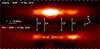 |
Fig. 1 Image of the disk at 12 µm, using a PCA reduction (bottom), and a Claslmg reduction performed with SpeCal. The disk has been rotated by 30 degrees in those images with respect to due north. Labels indicate the dust clumps described in Sect. 4. |
2.1.3 Post-processing
After the observations, frame selection was performed on the data cubes, based on the criteria of residual flux behind the coronagraphic mask. The 10% worst frames for which the star was slightly off-centered were rejected because otherwise resulting in poor stellar subtraction during the next step. After frame selection, the remaining on-source telescope time (behind the mask) is about 5060 s. We took advantage of the SPHERE Calibration Tool, SpeCal (Galicher et al. 2018), which can be easily adapted to any instrument by providing minor modifications of the input data to match the SpeCal format. SpeCal has been developed to accurately detect the faintest point sources in high-contrast imaging data, offering several types of algorithms for data analysis, such as angular differential imaging (ADI; Marois et al. 2006) combined with principal component analysis (PCA; Soummer et al. 2012) or TLOCI (Lafrenière et al. 2007). The simplest processing provides a direct stacking of frames once compensated by the field rotation. This is the classical averaging described in Galicher et al. (2018, Claslmg, for classical imaging). Figure 1 presents the resulting images, after a Claslmg and PCA reduction.
2.2 VISIR archival data
Non-coronagraphic observations of β Pictoris were obtained with VISIR on 2004 – program ID 6O.A-9234(A) – and 2015 – program ID 95.C-O425(A) – with the VLT. The observations were performed in a standard chopping-nodding mode. The data were reduced by combining all the chop-nodded frames into a single one. Each observation was typically 1 h long. The data were consequently flux calibrated by observing with the same settings an infrared standard (HD 42540, spectral type K2/3III, J = 2.90, H = 2.24, K = 2.09) just before the β Pictoris observations. The reduced data are further examined in Sect. 5 to perform a comparison with the NEAR observations.
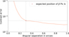 |
Fig. 2 Contrast curve at 5σ as measured along the disk spine across a width of 1″, as measured on the PCA image. The contrast of β Pic b with respect to the star and its distance to the star is indicated by the grey lines. |
3 Searching for β Pictoris b
3.1 A non-detection at mid-infrared wavelengths
Using various SpeCaľs algorithms, we performed several tests to reduce the stellar contribution and to reveal the expected planet. We compared the contrast curves provided by the cADI, Claslmg, PCA, and TLOCI algorithms: we found that the PCA reduction provides the deepest contrast curves at the expected separation of the planet. All the assessments provided a non-detection outcome, preventing us from identifying the giant planet β Pictoris b in the NEAR data. Observations obtained at a similar epoch with SPHERE yielded an angular separation of 301 ± 4 mas with respect to the star (Lagrange et al. 2020). At such a distance, which corresponds to 1 × λ/D at this wavelength (λ = 11.25 µm), the AGPM coronagraph would transmit only 32% of the flux of a point-source (see Fig. A.1). Taking this parameter into account, we further explored the sensitivity to point sources by injecting fake planets built from the non-coronagraphic star’s image at various contrasts, and processed with a set of ADI algorithms. We concluded that the PCA algorithm is providing the best contrast with ten modes removed.
One of the SpeCal output provides an estimation of the azimuthal contrast level for each angular distance. Therefore, we estimated the limit of detection in the PCA image. We note that the disk itself and the background are the major contributions to the noise, far beyond the speckle noise. The transmission curve of the coronagraph was computed by comparing the maximum intensity of the coronagraphic image at an increasing separation from the center, normalized to the PSF (non-coronagraphic) maximum intensity (Fig. A.1). Figure 2 shows the 5σ contrast curve corrected from the coronagraphic transmission. The contrast at the expected position of the planet β Pic b at 0.3″ is 5× l0−3.
3.2 Upper-limit constraints on the spectral energy distribution
The spectral energy distribution of β Pic b has been studied in a number of papers (Bonnefoy et al. 2011, 2013, 2014; Currie et al. 2013; Morzinski et al. 2015; Baudino et al. 2015; Chilcote et al. 2017; GRAVITY Collaboration 2020). The purpose of this section is not to carry out a similarly detailed analysis, but instead to perform an order of magnitude comparison between the detection limit presented in Sect. 3.1, by using atmospheric models predictions, determined from the planet’s flux in the near-IR.
First of all, we calculated the stellar flux density Fλ by assuming a BT-NEXTGEN1 model at Teff = 8000 K, log g = 4.0, with solar metallicity, as in Chilcote et al. (2017), together with a star’s radius of 1.65 R⊙ and a distance of 19.6 pc (EDR3; Gaia Collaboration 2021). Further, this stellar model was normalized to match the actual photometry of β Pic A (Bonnefoy et al. 2013). As for the planet spectral energy distribution, we used broad bands and narrow bands data (Y to M) from Bonnefoy et al. (2013), as well as the Gemini Planet Imager (GPI) spectrum presented in Chilcote et al. (2017) renormalized to the estimation of the star’s flux density from Bonnefoy et al. (2013). These photometric data are displayed in Fig. 3.
The upper limit of the planet contrast measured at 11.25 µm (the NEAR wavelength) translates to a flux density of 1.146 × 10⁻¹⁶ Wm−2 µm−1. A straightforward comparison with a BT-Settl model of the planet at Teq = 1600 K and log g = 3.5 unambiguously shows that the non-detection with NEAR does not allow to put meaningful constraints on the planetary atmospheric properties, the upper limit of the observed flux density being about three times larger than the model’s expectation from the near-IR detection (Fig. 3).
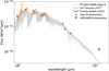 |
Fig. 3 Spectra of β Pictoris b obtained by fitting forward BT-Settle models to data obtained with several instruments (color-coded in the legend). The upper flux limit of the NEAR data is marked by a green triangle. |
3.3 Exploring the presence of circumplanetary material
3.3.1 Context
We often assume young giant planets to often be surrounded by a circumplanetary disk that later accretes onto the planet and produces satellites. The satellite-forming process is expected to leave a gas-free dusty disk, consisting of ring structures filling the planet’s Hill sphere, which will eventually disperse. A 18 Myr-old planet like β Pic b could still be surrounded by such a fading, and now optically thin circumplanetary disk. The planet’s Hill sphere has been indicated as a potential explanation for a ~4% photometric variation observed in 1981 (Lecavelier Des Etangs et al. 1995). However, continuous monitoring of the expected 2017 and 2018 Hill sphere stellar transits was not able to detect flux variation due to circumplanetary material (Kenworthy et al. 2021); instead, it could place an upper limit of ~l.8 × 1019 kg of dust in the planetary Hill sphere. We aim to investigate to what extent our 12 µm non-detection could place an upper limit on the amount of circumplanetary material. We recall that the angular resolution of NEAR at 11.25 µm corresponds to a patch of 5–6 au, which is much larger than the Hill radius of the planet (about 1.2 au for β Pic b), so that any circumplanetary material will appear unresolved.
This prevents us from constraining any further the dust’s spatial location and its size distribution around the planet. Consequently, by considering simple but physically relevant assumptions on the dust location and grain size distribution, we investigate the possible order of magnitude of the total dust mass that agrees with the flux upper limit measured at the planetary location.
3.3.2 Model
Schematically, at a given wavelength λ, dust grains are efficient emitters or scatters provided they have a radius, sdust that is on the order of sλ ~ λ/2π. For the NEAR filter, we calculated sλ = 1.9 µm, which is a value relatively close to the minimum size, Sblow, below which grains are blown out of the system by stellar radiation pressure. In fact, if we assume that grains are produced from progenitors on a circular orbit, then such grains will be ejected if the ratio β between radiation pressure and stellar gravity is higher than 0.5. Taking the standard expression for β given by Krivov (2010):
![Mathematical equation: $\beta \approx {{0.57} \over {{s_{{\rm{blow}}}}\left[ {{\rm{\mu m}}} \right]}}{1 \over {{\rho _{{\rm{dust}}}}\left[ {{\rm{g}}\,{\rm{c}}{{\rm{m}}^{ - 3}}} \right]}}{{{L_ \star }{M_ \odot }} \over {{L_ \odot }{M_ \star }}},$](/articles/aa/full_html/2023/07/aa45143-22/aa45143-22-eq3.png) (1)
(1)
with M⋆ and L⋆ being the mass and luminosity of the central star, and assuming ρdust = 2.7 g cm −3, typical astrosillicates density, L⋆ = 8.7 L⊙ (Crifo et al. 1997) and M⋆ = 1.77 M⊙ (Lagrange et al. 2020), we get sblow ≈ 2.1 µm.
By making the assumption that grains are produced by a col-lisional cascade starting from larger planetesimal-like bodies (be it in a circumstellar cloud or disc), then we can assume that they follow a standard size distribution in dn = s−35 ds down to s = sblow2. For such a distribution, the geometrical cross-section is dominated by the smallest grains just above sblow (Thebault 2016). Since sλ ~ sblow, this also means that the flux at λ is dominated by the smallest grains in the size distribution. For the sake of simplicity, we thus consider here a single-sized dust distribution made of sdust = 2 µm grains.
To estimate the temperature Tdust and flux F(Tdust) emitted by each dust grain, we consider the framework of the Mie theory for compact astrosilicate grains and use the GRaTer radiative transfer code (Augereau et al. 1999; Olofsson et al. 2020) to estimate the absorption coefficient, Qabs. We note that we here have two heating sources for the grains: the radiation from the star and the radiation from the warm young planet. Given the estimated temperature of the planet (~ 1700 K; Bonnefoy et al. 2013), the stellar parameters of β Pictoris, and the separation of 9.8 au between the host star and the planet, we find that grain heating by the planet dominates up to a distance ~100 RJ from the planet and that the stellar heating dominates beyond that. At the tipping point between these two domains, the grain temperature is of the order of Tdust ~ 140 K (Fig. 4).
We now assume that a grain emits as a black body weighted by Qabs, according to the temperature previously determined. Since the dust scattering at mid-IR is negligible against the emission, the flux re-radiated by a dust particle is as follows:
 (2)
(2)
with dpd being the distance planet to dust, c being the speed of light, h being the Planck constant, and k being the Boltzmann constant.
Considering the flux upper limit on the planet position (derived in Sect. 3), Flimdet = 1.146 × 10⁻¹⁶ Wm−2 µm−1 and in the optically-thin hypothesis, we then derive, at each radial distance from the planet, the maximum number of 2 µm-size dust particles as Ndust = Flimdet/F(Tdust, λ).
For spherical grains, the corresponding total mass of dust Mdust is then:
 (3)
(3)
which we can convert to an equivalent radius of a spherical parent body, Rparent, of the same density:
 (4)
(4)
We summarize our results in Fig. 5, which plots Mdust and Rparent as a function of radial distance to the planet up to the Hill sphere limit RHill at ~ 1.2 au, defined as:
 (5)
(5)
with aplanet as the planet’s semi-major axis, Mplanet as the planet’s mass, and M⋆ as the mass of the central star.
We see that within the 100 RJ radius domain, where heating is dominated by the planet, the dust mass required to emit Flimdet increases with increasing distance from the planet. Such a result was expected due to the dust temperature decrease observed within this domain (Fig. 4). On the contrary, in the region beyond ~100 RJ, where stellar heating dominates, both Mdust and Rparent stay constant. This means that, within the simplified frame of our model, it is impossible to distinguish between dust located at 100 RJ ~ 7.15 × 10⁶ km and RHill ~ 1.78 × 10⁸ km. Interestingly, the value of Mdust ~ 5 × 10¹⁸ kg that we derived in the stellar radiation-dominated domain is relatively close to the upper limit of 1.8 × 10¹⁹ kg derived by Kenworthy et al. (2021) during the hypothetical transit of the Hill sphere of the planet in 2017-2018 (displayed as a dotted green line in Fig. 5).
We note, however, that we obtained different dust mass constraints in the more compact planet-heating dominated domain. For example, if we consider the case of a planetary ring extending out to the Roche radius at ~2.7 RJ, then the maximum dust mass value would be only ~2 × 10¹⁵ kg, corresponding to the mass of a ~5 km-sized object. This is ~700 times less than the estimated mass in Saturn’s ring (Iess et al. 2019), so we can rule out the presence of a massive Saturn-like planetary ring around β Pictoris b.
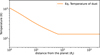 |
Fig. 4 Dust equilibrium temperature, calculated with Mie theory, of a 2 µm grain particle located within a radius of ~ 100 RJ from β Pictoris b and assumed to be constant further out up to RHill. |
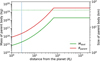 |
Fig. 5 Mass (green line) and size (red line) of a parent body able to produce by collision a cloud of dust of which the emitted flux in the NEAR bandpass could be compatible with Flimdet at the planet position. The green dotted line represents the upper limit of Kenworthy et al. (2021). The blue dotted line stands for the Roche limit. |
4 Dissecting the disk morphology
In this section, we present and analyze the morphology of the disk structures as observed at mid-IR wavelengths with NEAR-VISIR. The β Pictoris disk is seen edge-on and extends to a projected separation of ~5″ that is equivalent to about 100 au. Figure 1 presents a cropped, rotated image of the disk, corresponding to the 2019 observations with NEAR, for two different reduction methods. The Claslmg reduction (described in Sect. 3.1) performs a derotation and averaging of the frames, while PCA provides better rejection of the starlight, but comes with self-subtraction artifacts (Milli et al. 2012). The Claslmg image has the advantage to preserve the disk photometry and morphology, but the star’s diffraction pattern dominates at short separations (< 0.75″). The disk image in the thermal regime features notable structures in the form of several clump-like patterns, as indicated in Fig. 1. In particular, the southwest (SW) clump, labeled CI, discovered in previous studies (Telesco et al. 2005; Li et al. 2012), and located at a separation of ~2.8″ (projected distance of ~55au), is the most obvious feature in the image. Another clump (C2) is visible in the northeast (NE) side at a position of ~l.7″ (projected distance of ~33 au). Cl and C2 are both rather broad with a full width at half maximum of ~ 1.3″ and ~0.8″, respectively. Although they were only marginally detected, we also identified two more clumps: C3 at the SW (1.5″ equivalent to a projected separation of ~3O au) and C4 in the NE (0.8″ equivalent to a projected separation of ~l6 au that is less than 3λ/D). Still, the reliability of C4 as a real disk structure may need further confirmation to disentangle from diffraction residuals. Contrary to near IR observations, the NEAR image does not reveal any sign of the warp (Mouillet et al. 1997), a feature that is only observed in scattered light.
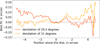 |
Fig. 6 Spine of the disk measured in the Claslmg image for the two position angles minimizing the disk slope in the northeast (PA = 31.0°) and in the southwest (PA = 29.5º). The y-axis: departure ſrommidplane in arcseconds. The x-axis: stellocentric distance in arcseconds. |
4.1 Orientation of the disk spine
Measuring the position angle of the disk sets the base of its analysis. We used a similar method as in Lagrange et al. (2012), Milli et al. (2014), and Boccaletti et al. (2018) to extract the disk spine and derive the global position angle of the disk. From the PCA image, we assumed a range of position angles around a guessed position (θ = 30°, Δθ = 6°, and δθ = 0.1°) and derotated the image by the complementary angle to position the disk near the horizontal orientation. The spine is defined as the departure from the mid-plane and is extracted by perpendicularly fitting a Gaussian profile at each stellocentric distance on both sides of the star. The local slope of the disk spine is measured at different positions along the spine, away enough from the center to avoid the bias from the self-subtraction induced by the PCA reduction. Averaging the values, typically ranging from 1.5″ to 4.0″, we searched for disk position angle that nulls down the slope. In Fig. 6, we show the disk spine for the two values minimizing the slope in the northeasterly and southwesterly regions, which are 31.0° and 29.5°, respectively; these values are in relatively good agreement with the position angle measured at L band by Milli et al. (2014). We adopted an averaged value of 30.0° ± 0.5°, which appears discrepant with regard to the one used by Telesco et al. (2005); however, applying the same method to measuring the PA in the VISIR data of 2004 and 2015 leads to a result of ~33.3º ± 1o and ~34.4º ± 1o, respectively. As a reference, the most accurate value measured in scattered light owing to precise astrometric calibration is 29.2 ± 0.2° (Lagrange et al. 2012). The most notable difference of several degrees with the NEAR 2019 data could be related to the lack of an astrometric calibration procedure related to these data, especially since VISIR was moved to the VLT UT4 for the NEAR experiment. Still, this mismatch has no impact on the following analysis.
We note that in scattered light images, the midplane and the warp are observed as two distinct components owing to the edge-on orientation combined with the radiation pressure effect (Golimowski et al. 2006; Lagrange et al. 2012). Milli et al. (2014) have also referred to a warp in the L band, while, in fact, the disk image shows a single component that reveals a very similar trend to the one observed in the mid-IR: a single disk component with a misalignment on the two sides. Moreover, a larger PA in the mid-IR has also been reported by Pantin et al. (2005), both in the N and Q bands. One possible interpretation can be drawn from temperature effects. Grains that are closer to the stars, thus, located inside the warp (≲8O au), dominate the global emission. In addition, the warp can be collisionally more active than the outer part of the disk due to the planet’s gravitational influence, β Pic b, onto the planetesimals, with a higher rate of small grains released, and with the latter acting as efficient emitters. As a result, the mid-IR image of the disk would be essentially oriented along the warp.
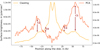 |
Fig. 7 Surface brightness profile of the PCA image (red), and Claslmg image (orange). The y-axes correspond to the Claslmg on the left and the PCA on the right. Labels of the clumps have been added for convenience. |
4.2 A clumpy structure
To analyze the clumpy structure of the disk, we converted the images to intensity units in Jy arcsec−2, by taking into account the pixel area (a dilution factor of 2 × 10⁻³ corresponding to 1/pixel_scale2) and a photometric calibration which gives a total flux in the coronagraphic image of 1.1 × 10⁶ ADU for a point source of l Jy. The surface brightness of the disk is obtained by integrating the intensity values for each pixel slice, of 12 pixels wide (0.54″), encompassing the disk thickness, and perpendicular to the mid-plane.
Figure 7 presents the resulting intensity profile along the disk for the Claslmg and PCA processing. The clumps CI and C2 can be identified in the surface brightness profiles, both in the Claslmg and PCA case. To a lesser extent, the hypothetical structures C3 and C4 are barely visible in the surface brightness. As visible in Fig. 1, the PCA reduction considerably attenuates the stellar contribution, impacting the photometry of the disk due to self-subtraction, with a stellocentric dependence. We note that the clumps, in particular C1 and C2, are very elongated and that being seen edge-on there is an obvious degeneracy between radial and azimuthal extension (or possibly both). C1 has a projected width of ~30au as seen in Fig. 11, with a sharper width of ~ 10 au, corresponding roughly to the width of the peak in the PCA profile.
5 Temporal evolution of the southwest clump C1
The β Pictoris system has been observed in the mid-IR on several occasions with 8-m class telescopes since December 2003, when C1 was first identified by Telesco et al. (2005). Given the 16-yr baseline with respect to our NEAR observations, the study of its evolution becomes relevant and can potentially allow us to address questions around its origin. Table 1 presents the data available in the mid-IR that we used for comparison with our data set. Both Telesco et al. (2005) and Li et al. (2012) located the position of С1 by performing a centro-symmetrical subtraction of the disk image, subtracting the emission in the fainter NE wing from the SW wing, and vice-versa. This yielded a residual emission, which was then assumed to be the main contribution of the clump. Indeed, in images without AO, the resolution is such that it is difficult to isolate the clump without this specific processing. For consistency reasons, we processed the 2004 and 2015 VISIR data similarly (Fig. 8). In comparison, in the 2019 data, C1 is unambiguously detected and resolved, as seen in Fig. 1, without any particular processing. This further emphasizes the efficiency of the use of AO along with a coronagraph.
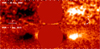 |
Fig. 8 Images of the centro-symmetrical subtraction of the disk at 11.25 µm, obtained with VISIR in 2004 on VLT UT3 (top) and at 11.7 µm obtained in 2015 (bottom). In both images, the disk has rotated, respectively, 33° and 34° with respect to the north. |
5.1 Impact of the centro-symmetrical subtraction
Measuring the exact position of C1 from the intensity profile is not straightforward, given the width of the clump of several au. In the following, we assume that the position of С1 is driven by the intensity peak of this structure and we did not make any assumption on whether it is radially or azimuthally extended. Furthermore, as we used either PCA or centro-symmetrical subtraction, any stellar residuals or the main disk emission itself do not impact the determination of the C1 position. In order to verify that the centro-symmetrical subtraction does not impact the position of C1, especially given the presence of the clump C2 and that the stellar contribution is substantial, we performed a measurement in the Claslmg 2019 image after applying the same centro-symmetrical subtraction.
We found that the results of the two methods (centro-symmetrical subtraction in Claslmg vs. PCA ADI) are consistent within ±0.1 au (corresponding to approximately ±0.1 pixel), confirming the accuracy of the former method, as seen in Fig. 9. Hence, we did not apply the centro-symmetrical subtraction to determine the location of С1 in the 2019 data.
Summary of the data used and the observing modes with different instruments.
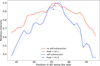 |
Fig. 9 Comparison of methods for measuring the position of C1 in the 2019 data. Red curve corresponds to the relative intensity from the PCA image, while the blue curve corresponds to the centro-symmetrical self-subtraction of the disk, from the same PCA image. Both methods provide the same result ±0.2 au. The position was measured by doing a Gaussian fit on the peak. The two curves have been normalized to make the comparison more visible. |
5.2 Position and error bar estimations
We considered the following sources of uncertainty in measuring the position of C1 and we describe the resulting errors for each of these contributions to the 2019 data.
The first source of error comes from estimating the position of the star in the image. We performed this estimation by doing a Gaussian fit of the center of the image in the Claslmg process, compared to the center of the image. The residual error is coming from the derotation of the images in the Claslmg process, when assuming the star is centered on the image. We estimated a resulting 0.2-pixel error corresponding to the cumulative error in the Claslmg sequence. This includes QACITS pointing control error, which centers the star on the coronagraph within ~0.02 λ/D.
The second error comes from the measurement of the orientation of the disk: repeating the process of measuring the clump position for the range of PA (30° ± 0.5°), we found a dispersion lower than 0.3 pixel.
The third source of error lies in the Gaussian fitting of the clump: to accurately measure the position of the clump, we limited the range of distance from the star where we fit a Gaussian profile (from around 2″ to 4″) centered approximately on C1, as seen in Fig. 10). The resulting error is 0.1 pixel.
Finally, the data reduction method induces biases. First, the PCA reduction introduces a bias leading to a photometric error; furthermore, the centro-symmetrical subtraction performed for the 2004 and 2015 data adds up. To estimate the bias introduced by the PCA reduction, we compared the position of C1 with the one found with the Claslmg reduction by performing a centro-symmetrical subtraction, resulting in a shift of 0.1 pixel.
Taking these factors into account, the total uncertainty for the 2019 data corresponds to the quadratic sum of each contribution, which equals 0.34 pixels (equivalent to 0.3 au).
With regard to the 2015 data, the same sources of uncertainty were considered for the error estimation, except that QACITS was not used for the centering. The centering error is of ~0.3 pixels, due to the bright PSF making it more challenging to accurately locate the star center as compared to the 2019 data. As for the position angle of the disk, the error is estimated to be lower than 0.3 pixels as well, as long as the same method as the 2019 data was applied. The error induced by the starting points of the Gaussian fit is 0.1 pixel. Here, the centro-symmetrical subtraction is another contribution to the error, which is estimated to be 0.1 pixel (cf. Fig. 9). The resulting uncertainty corresponds to 0.45 pixel, corresponding to 0.4 au.
The 2004 data follows the same error estimation calculations as the 2015 data, with a difference coming from the pixel scale of the detector being different (0.075 arcsec pix−1, instead of 0.045 arcsec pix−1 for 2015 and 2019, respectively, following a sensor upgrade). The resulting uncertainty corresponds to 0.6 au.
In conclusion, the C1 projected distances for the 2004, 2015, and 2019 data are 52.7 ± 0.6 au, 55.5 ± 0.4 au, and 56.1 ± 0.3 au, respectively. These results are summarised in Table 1.
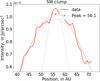 |
Fig. 10 Position of С1 in the PCA image of the 2019 data. Two Gaussian curves have been added in dashed lines to show the substructures within the disk and the brown line corresponds to the final fit. |
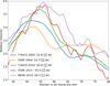 |
Fig. 11 Evolution of the projected distance and relative intensity profile of C1 over the years, from different instruments (colour-coded in the legend). The intensity for the VISIR and NEAR data has been set to scale with the T-ReCS data by Li et al. (2012). |
5.3 Temporal evolution of C1’s projected distance
Figure 11 presents the intensity profiles of the disk for each epoch around the location of C1. The T-ReCS measurements from 2003 and 2010 were obtained from the plots in Telesco et al. (2005) and Li et al. (2012), after updating the star’s distance to 19.63.
The apparent projected separation of the clump is clearly increasing over time, suggestive of a global outward motion of C1. This is even more obvious when plotting its measured position versus time on a 16-yr baseline, as in Fig. 12 (red circles for 2003 and 2010 data, red squares for 2004, 2015, and 2019 data). This outward motion of the projected distance is likely to be slowing down over time, indicating that the clump should be coming close to its maximum elongation.
We note that the overall profile of C1 has a two-mode shape with a nearly Gaussian part inward and a plateau outward, indicative that the actual three-dimensional shape of the clump is more complex. In particular, the clump can be azimuthally and/or radially extended. In the latter, the differential Keplerian rotation will modify the projected intensity profile with time, an effect which could already be suspected in Fig. 11. Furthermore, we considered studying the evolution of the size of the clump, however, the current data do not allow us to accurately quantify such evolution. Follow-up observations with similar or better angular resolution than NEAR will be key to future investigations of the actual morphology of the clump.
Carrying out a quantitative comparison of the disk intensity profiles is impractical, given the absolute flux is not known accurately enough in each dataset. For that reason, we normalized the profiles in Fig. 11 to roughly match the SW side intensities beyond 65 au, for the purposes of visualization.
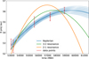 |
Fig. 12 Evolution of the position of C1 over the 16 yr of observations (red squares for VISIR and NEAR, red circles for T-ReCS). The best Keplerian model is overlaid in blue together with the 1-sigma dispersion (light blue), corresponding to |

Projected separations of the clumps observed with NEAR.
5.4 C1’s orbital radius
To set some constraints on the orbit of C1 – given the scarcity of data points, the small fraction of the orbit coverage, and the rather large error bars with regard to the clump location - we assumed a simplified configuration in which the clump orbit is circular and perfectly edge-on. Therefore, we purposely excluded the possibility of elliptical orbits since they would bring on too many solutions. In that case, the Keplerian angular velocity is expressed as:
 (6)
(6)
with a being the semi-major axis and G being the gravitational constant. The projected separation, x0, at the first epoch is given by:
 (7)
(7)
with θ0 defining the angle between the clump and the direction perpendicular to the line of sight. Since the Keplerian speed is constant for a circular orbit (ΩK = Δθ/Δt), the projected separation, x[t, a], as a function of time for a given orbital radius is expressed as:
![Mathematical equation: $x\left[ {t,a} \right] = a\cos \left( {{\theta _0} - t \cdot \sqrt {{{G{M_ * }} \over {{a^3}}}} } \right).$](/articles/aa/full_html/2023/07/aa45143-22/aa45143-22-eq16.png) (8)
(8)
To estimate the best models matching the data given the error bars, we generated a grid of 2000 models of two parameters, α and x0, with the following priors: 55–60 au (step 0.1 au) and 51.9–53.9 au (step 0.05 au), respectively. As a result of a χ2 minimization, we were able to constrain the semi-major axis of C1 to  au (and
  . More details are given in Fig. 12).
Telesco et al. (2005) measured a position for C1 of 52 au in December 2003, while Li et al. (2012) obtained 54 au, then speculated a displacement of roughly  au. The latter authors concluded that the clump is moving at Keplerian velocity, corresponding to an orbital radius of
  au. When considering a stellar distance of 19.63 pc (Gaia Collaboration 2021) instead of 19.28 pc, the orbital radius changes to
  au, according to Fig. 8 in Li et al. (2012). This is a value that ought to be compared to the obtained values described in the previous section. Therefore, our measurement is in agreement, within the error bars, with this revised value. We note that this value corresponds almost exactly to the projected separation of the clump in the 2019 data, hence, the clump is supposed to be at its maximal elongation.
6 Other clumps and comparison with ALMA
As mentioned in Sect. 4, the 2019 NEAR images of the disk feature additional clump-like structures. We measured the projected separations of these structures following the approach detailed in Sect. 5 for the clumps C2, C3, and C4. We obtained, respectively,  ,
,  ,
,  for the clumps C2, C3, and C4 positive towards SW and negative towards NE. Table 2 summarizes the clumps positions. The intensity profile of C2 is shown in Fig. 13. Similarly to the C1 clump, we fit a Gaussian curve on C2, to estimate its position making the assumption that the profile of the clump is Gaussian yielding a width of ~15 au.
Dent et al. (2014) and Matrà et al. (2017) observed the β Pictoris disk at submillimeter wavelengths with the Atacama Large Millimeter/submillimeter Array (ALMA), presenting the spatial distribution of the CO gas for the transitions J = 3–2 (resolution of 15 au) and J = 2–1 (resolution of 5.5 au). Both studies identified two clumps respectively to the SW (~5Oau) and the NE (~30au).
To assess to what extent these CO clumps match those we have identified here, we show (in Fig. 14) the superimposition of the projected intensity profiles for the NEAR 2019 data, together with the ALMA data. For consistency, we used the star’s distance of 19.63 pc for these three observations, thus including potentially slight differences with the two aforementioned papers regarding the positions of the structures. Although we detect with VISIR a well-resolved clump (C2) in the NE part of the disk, the correspondence with the CO gas distribution is not very conclusive. Not only does the clump on the NE side in ALMA images peak at about 25 au, as opposed to 33 au in the VISIR image, but it is also related to a much broader projected structure, especially in CO J = 3–2 (~70au), than at 11.25 µm. On the SW side, on the contrary, there is a good match between the projected location of C1 and that of the CO gas clump. A small offset (~6au) of C1 between ALMA and VISIR observations is visible in Fig. 14, but this cannot be attributed to the clump orbital motion according to the analysis in Sect. 5.4, possibly implying a slightly different distribution of the dust and gas components. However, we note that Matrà et al. (2017) argued that while the projected location of the CO clump is around 50 au, its deprojected stellocentric distance (deduced from position-velocity (PV) diagrams of CO intensity) peaks, in reality, at ~85 au. This seems to contradict the results of our orbital analysis (Sect. 5.4), which the semi-major axis of the dust clump is constrained to lie around 56 au. At face value, this would suggest that we are witnessing two different clumps whose projected positions happen to coincide. Such a conclusion should, however, be taken with great caution. The PV diagrams of the CO lines do indeed also suggest that the gas clump should be radially extended, spanning ~100au forthe orbital radius. If the dust clump was to have a similar radial extension, then it could appear brighter (because of higher temperatures) at its inner edge, while the peak CO luminosity could be located further out, thus explaining the apparent discrepancy. In addition, the different transitions of CO gas will be more or less excited depending on temperature and the density of collisional partners (in non-LTE as is the case for β Pic; Matrà et al. 2017) and they are not necessarily representative of the underlying CO or dominant gas species spatial distributions (e.g., Kral et al. 2016). These questions clearly go beyond the scope of the present paper, and we leave this to be an open issue for investigation in future studies.
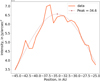 |
Fig. 13 Relative intensity along the disk in the PCA image, focused on C2. The intensity values were kept the same as in Fig. 11. |
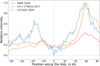 |
Fig. 14 Projected distribution of CO lines flux obtained from Dent et al. (2014) and Matrà et al. (2017), superimposed with the radial flux distribution of the disk at 12µm with VISIR. The VISIR and CO 3–2 (Dent et al. 2014) curves have beennormalized bytheirmaximum. |
7 Origin and fate of C1
As shown in Sect. 5.4, the location of C1 over the 2003-2019 period is compatible with a circular Keplerian orbit with a  au semi-major axis. During the review process for the present paper, Han et al. (2023) published a study arguing that the main SW clump (C1) ought to be stationary, which seems to contradict our conclusion. We note, however, that, while Han et al. (2023) constrained the maximum displacement of the clump to, indeed, be less than 0.2 au over a 12-yr period at the 1σ level, this value increases to 11 au at the 3σ level, which would be compatible with our own results (see Sect. 5.4). We also note that differences could arise from different approaches for pinpointing the clump’s location: we constrained it by looking for the peak luminosity location while Han et al. (2023) constrained it by performing a fit of the whole projected profile of the clump. Lastly, the present study considers a longer time baseline, with the 2019 NEAR data extending it to 16 yr instead of 12. Keeping in mind these possible caveats, we go on to review some possible scenarios for explaining the clump’s motion over time below.
7.1 Giant impact
Since its detection by Telesco et al. (2005), several explanations have been proposed for the presence of C1. The first is the catastrophic disruption of a large (~100 km) planetesimal (Telesco et al. 2005; Li et al. 2012). As demonstrated by Jackson etal. (2014) and Kral etal. (2015), the fact that the produced col-lisional debris are placed on eccentric orbits, all passing through the location of the initial break-up, produces a long-lived bright clump at this location. However, this clump stays at a fixed position with respect to the star, which does not agree with the observed motion of the clump over a 16-yr interval. The only way a catastrophic disruption leads to a moving clump is if it is observed in the immediate aftermath of the break-up, before the debris had time to perform a complete orbit (see, e.g., Fig. 7 of Jackson et al. 2014). While this possibility cannot be ruled out, it is very unlikely given the fact that such large disruptive events are known to be relatively rare (Wyatt & Jackson 2016).
7.2 Coiiisionai avalanche
Alternatively, Li et al. (2012) considered the possibility that given the large radial extension of the clump and the fact that it might contain sub-micron grains, it is the signature of a so-called collisional avalanche. This is a collisional chain reaction triggered by outward moving unbound small grains produced by the break-up of planetesimals closer to the star (Grigorieva et al. 2007). However, the duration of an avalanche event is relatively short, on the order of ~0.3 torb, again requiring the assumption that we are witnessing the immediate aftermath of a large plan-etesimal break-up (Thebault & Kral 2018). However, contrary to the “local” giant disruption scenario considered before, the avalanche-triggering planetesimal break-up would occur much closer to the star (at a typical asteroid-belt location), in regions where such events could be less rare, and would require the breaking up of a smaller body (Thebault & Kral 2018).
7.3 Resonance trapping by a pianet
Analyzing the characteristics of the CO clump discovered at roughly the same projected location as the dust clump, Dent et al. (2014) and Matrà et al. (2017) also ruled out a giant disruption event and favored instead a scenario in which the clump is the result of resonance trapping of CO-producing planetesi-mals by a planet moving with a Keplerian orbit. Such a scenario would imply that the clump moves at the angular velocity of the planet, that is, significantly faster than the expected Keplerian speed at the location of the clump. We tested this hypothesis by fitting the 2003–2019 clump positions when assuming that it moves at the angular speed of a planet with which it is in either a 3:2 or 2:1 resonance (the two cases considered by Matrà et al. 2017). As shown in Fig. 12, a 2:1 resonance can be confidently ruled out (reduced minimal  , while a 3:2 case might be marginally possible (reduced minimal
  given the error bars. Still, the scenarios with resonances are significantly worse than when assuming the local Keplerian orbit (reduced minimal
  , Fig. 12). We note that for this 3:2 resonant scenario, any new observation of the clump location should easily settle the validity of this hypothesis.
7.4 Planet’s Hill sphere or trojans
The most likely hypothesis we are left with is thus that of a dust clump that orbits at the expected local Keplerian speed and should be relatively long-lived in order to be observed. If this clump is linked to the presence of a yet-undetected planet, then it could be either circumplanetary material within the planet’s Hill radius or Roche lobe or, alternatively, material trapped in the corotating L4 or L5 Lagrangian points, in a Trojan-like configuration. Telesco et al. (2005) estimated the total mass of dust in the clump to be around 4 × 10²⁰ g, which is much less than the estimated mass of the Jupiter Trojans, ~6 × 10²³ g (Jewitt et al. 2000). However, 4 × 10²⁰ g is the estimated mass of dust (typically ≤1 mm), whereas the estimated mass of Trojans is that of ≥1 km objects. If we assume that the observed dust is produced by a collisional cascade starting at ~1 km object, with a differential size distribution following a power law of index q = −3.5, then we get an extrapolated total mass of ~4 × 10²³ g, which is roughly comparable to the mass of km-sized Jupiter Trojans. There is, however, a potential issue with this scenario if the dust clump has the same radial extent as that of the clump seen in CO. The relative radial width of the stable region around the L4-L5 points should indeed not exceed ~10% (Liberato & Winter 2020), whereas it is at least ~5O% for the observed CO clump (Matrà et al. 2017). As discussed in Sect. 6, the correspondence between the dust and CO clumps is a complex issue that is left to future investigations. We remain careful as we stress that the Trojan scenario might be challenged by a radially broad dust clump.
Another possibility is that the clump is confined within the Hill sphere surrounding a planet. In this case, the minimum mass of the putative planet can be derived from the size of the clump, using Eq. (5) and assuming that the clump is smaller than RHill. For a typical clump size of ~10 au, the mass of the planet having a Hill sphere of this size is of the order of 3 MJ. The problem is that, at a distance of ~50 au, such a massive planet would have had a 99% probability of having been detected by Lagrange et al. (2020) with a combination of radial velocity and imaging. This problem could be overcome if the clump is optically thick (τ > 1) and, thus, it would be hiding the planet’s photosphere. For a 10 au wide clump made of the smallest possible grains (~2 µm), the τ > 1 criteria would lead to a minimum clump mass of ~5 × 1025 g, which corresponds to the mass of a Moon-sized object.
7.5 A vortex
In the hypothetical case that the gas and dust clumps are co-located, a scenario that could allow for a somewhat large radial extent (as deduced from observations of the gas velocity Matrà et al. 2017), while also explaining that the gas orbits at the local Keplerian velocity are those characterizing a vortex. Vortices have been extensively studied, both analytically and numerically, in the context of younger protoplanetary disks, yet they have never been proposed as an explanation for clumps in debris disks. There are several ways to generate vortices in disks, but large-scale vortices are most often thought to arise from the Rossby-wave instability (RWI). This instability can set in when there is a radial minimum in the gas potential vorticity, which, in practice, can happen when there is a radial maximum in the gas pressure (see, e.g., the review by Lovelace et al. 2013).
Radial pressure maxima could well occur in debris disks. The pressure maximum could be related to: (1) a Saturn-like planet or more massive creating a gap with a natural pressure maximum at its outer edge (just like in a gas-rich protoplanetary disk; see, e.g., Hammer et al. 2021); (2) the presence of a clump of solids (similar to that observed in β Pic) that releases gas and naturally creates a pressure maximum. Large-scale vortices can also survive for thousands of orbits, namely, millions of years at > 50 au (Hammer et al. 2021), making it possible to observe in a ~20 Myr-old system. We note, however, that the typical lifetime of vortices depends, among other things, on the gas turbulent viscosity, with smaller turbulent viscosities favoring longer-lived vortices (see, e.g., the discussion in Sect. 4.2 in Baruteau et al. 2019). The amount of turbulence in debris disks is not yet obser-vationally constrained but it could be very high in low-gas mass ionized systems and lower in more massive disks (Kral & Latter 2016).
According to current RWI models, the smallest dust with a Stokes number of ~ 1 (~ µm dust) is expected to have a tendency to concentrate near the center of the vortex, but the effect of radiation pressure, which cannot be neglected in debris disks, has not been taken into account in RWI models and may alter this conclusion. We also note that when the dust-to-gas mass ratio in the vortex becomes greater than 0.3–0.5, the vortex may be destroyed (Crnkovic-Rubsamen et al. 2015). In the case of β Pic, Kral et al. (2016) calculated that the dust-to-gas mass ratio is greater than 1 beyond 20 au, so this effect of dust feedback on the gas vortex may be relevant here.
The presence of a vortex would also solve another as-yet unexplained phenomenon, namely, that the neutral carbon gas observed with ALMA is not axisymmetric (as predicted by the models) but clumpy, similarly to what is observed for CO (Cataldi et al. 2018). Indeed, according to current models, CO should photodissociate in less than one orbit, which may explain why it is clumpy (Matrà et al. 2017), but the carbon that is created due to the photodissociation of CO should instead become axisymmetric rapidly on a time scale of a few orbits. On the contrary, if the gas forms a vortex, both the carbon and CO are indeed expected to be clumpy. The large width of the clump is also in line with the idea of a vortex in the gas. An RWI-induced vortex has indeed a radial width that is typically twice the local pressure scale height (Baruteau et al. 2019) and can thus reach tens of au, as observed for β Pic.
We also note that a significant brightness asymmetry is observed in the near IR (e.g. Apai et al. 2015) and a clump in the mid-IR (Telesco et al. 2005, and this study) but not in the mm (Matrà et al. 2019). This could also be explained by the presence of a vortex trapping only the smallest µm-sized grains (with a Stokes number ≲1), while the largest mm-grains would remain unperturbed by the vortex and retain a near axisymmetric spatial distribution. These statements should be further analyzed via numerical simulations in a dedicated study.
Although further numerical simulations for the specific case of debris disks are needed to strengthen our conclusions, vortices are compelling contenders for explaining the results of observations and they deserve more attention in the context of β Pic, as this would allow us to explain (for the first time) the observations of CO and carbon gases as well as the observations of dust in the near- and mid-IR, as well as in the mm. For all these reasons, we suggest that it is a viable scenario that needs further theoretical and observational testing.
If we expect C1 to be caused by a vortex formed at the outer edge of the annular gap of a planet, we could offer an idea of where the planet would be located according to its mass. A vortex formed at the outer edge of a planet’s gap is typically located within a few (5–10) Hill radii of the planet. For a Jupiter-mass planet around a Sun-mass star, the vortex will have a semi-major axis ~1.5 a (see for instance Fig. 2 by Baruteau et al. 2019). In our case, the hypothetical planet would be located around 37 au (assuming a dust clump centered at ~50 au), which is between C3 and C1.
8 Conclusion
This paper presents the first high contrast imaging data in the mid-IR of the β Pictoris system, observed with NEAR. Here, we summarize the main results of our analysis of these data, along with a comparison with previous observations.
The planet β Pictoris b was not detected with NEAR. However, by taking into account the transmission of the coron-agraph, we derived the planetary flux upper limit from the contrast curve at 5σ. We collected spectro-photometry from different instruments and presented a combined spectrum the first spectra of β Pictoris b acquired with SPHERE during several epochs. The upper limit of the NEAR data does not allow us to put meaningful constraints on atmospheric scenarios.
Given the upper limit on the planetary flux, we investigated which corresponding amount of dust, present around the planet, could reproduce such a limit. Although this quantity scales with the distance to the planet, we concluded that the presence of a dust cloud around the planet was unlikely. If dust particles were located at the Roche radius, it would correspond to the collisional debris of a 5 km size asteroid.
The disk is uniquely resolved in these mid-IR data, allowing us to identify structures that were never observed prior to those observations. The southwesterern clump, previously reported in the literature, is distinctively detected in the NEAR data set, at
 au. On the northeastern side of the disk, there is a clear detection of a new clump at
  au. We note the possible presence of two other clumps at
  au at
au at  au. Further observations will be required to confirm their existence.
The southwest clump was observed several times since its discovery in 2003, with T-ReCS and VISIR. The 16-yr baseline of observations, with five observing sequences, allowed us to assess the motion of the clump over time, and to confirm a Keplerian behavior. This result is based on the assumption that the clump has a circular orbit, which would be challenged in the case of an elliptical orbit.
We investigated qualitatively different origins for the southwest clump, in particular, the possibility that it could be the Hill sphere of a yet-to-be detected planet with a maximum mass of 3MJ. Given the fact that it is in motion, we ruled out the scenario that this clump is the result of a giant impact. We have provided arguments for a scenario where the clump would be a dust-trapping gas vortex, based in particular on the possible superimposition of the southwest clump and the CO clump seen with ALMA.
The β Pictoris system has been extensively studied at different wavelengths and it serves an archetypal system for our understanding of planet-disk interactions and planetary formation. This study shows that the use of adaptive optics, along with a coronagraph in the N band, does bring a considerable improvement with regard to the data quality. The NEAR data have allowed us to put constraints, for the first time, on the presence of circumplanetary material around a directly imaged planet. We could indeed expect giant planets to have circumplanetary disks, as all the giant planets in our solar system do indeed have some. Similarly, we detected disk structures that had never been observed before. Further observations are needed to confirm some of those structures and understand their origin. Likewise, further observations of C1 are needed to track its evolution and confirm its origin, and to put better constraints on the evolution of the size of the clump. The James Webb Space Telescope will provide unique mid-IR data that will significantly help us in improving our understanding of the famous β Pictoris system.
Acknowledgements
We want to thank the ESO, the Breakthrough Foundation, and everyone involved in the NEAR project. The observations were carried out under the ESO program id: 60.A-9107(K). We want to thank the referee for the constructive feedback that contributed to improving the quality of this paper. N.S. acknowledges support from the PSL IRIS-OCAV project. This project has received funding from the European Research Council (ERC) under the European Union’s Horizon 2020 research and innovation programme (COBREX; grant agreement #885593). French co-authors also acknowledge financial support from the Programme National de Planétologie (PNP). We thank J. Chilcote for sharing the GPI spectrum of β Pic b. C.D. acknowledges financial support from the State Agency for Research of the Spanish MCIU through the “Center of Excellence Severo Ochoa” award to the Instituto de Astrofísica de Andalucía (SEV-2017-0709) and the Group project Ref. N.H. was partially funded by Spanish MCIN/AEI/10.13039/501100011033 grant PID2019-107061GB-C61 and No. MDM-2017-0737 Unidad de Excelencia María de Maeztu - Centro de Astrobiología (CSIC-INTA). PID2019-110689RB-I00/AEI/10.13039/501100011033.
Appendix A Transmission of the coronagraph
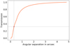 |
Fig. A.1 Transmission of the AGPM coronagraph as a function of the separation, simulated by scanning a point source radially with respect to the center of the coronagraph. The transmission is measured in the central pixel of the point source image and normalized to the unattenuated PSF. The transmission at the expected position of the planet β Pic b, at 0.3”, is 32%, identified as a brown dot in the plot. |
References
- ALMA Partnership (Brogan, C. L., et al.) 2015, ApJ, 808, L3 [Google Scholar]
- Apai, D., Schneider, G., Grady, C. A., et al. 2015, ApJ, 800, 136 [NASA ADS] [CrossRef] [Google Scholar]
- Arsenault, R., Madec, P. Y., Vernet, E., et al. 2017, The Messenger, 168, 8 [Google Scholar]
- Augereau, J. C., Lagrange, A. M., Mouillet, D., Papaloizou, J. C. B., & Grorod, P. A. 1999, A&A, 348, 557 [NASA ADS] [Google Scholar]
- Augereau, J. C., Nelson, R. P., Lagrange, A. M., Papaloizou, J. C. B., & Mouillet, D. 2001, A&A, 370, 447 [NASA ADS] [CrossRef] [EDP Sciences] [Google Scholar]
- Baruteau, C., Barraza, M., Pérez, S., et al. 2019, MNRAS, 486, 304 [Google Scholar]
- Baudino, J. L., Bézard, B., Boccaletti, A., et al. 2015, A&A, 582, A83 [NASA ADS] [CrossRef] [EDP Sciences] [Google Scholar]
- Beuzit, J. L., Vigan, A., Mouillet, D., et al. 2019, A&A, 631, A155 [NASA ADS] [CrossRef] [EDP Sciences] [Google Scholar]
- Boccaletti, A., Sezestre, E., Lagrange, A. M., et al. 2018, A&A, 614, A52 [NASA ADS] [CrossRef] [EDP Sciences] [Google Scholar]
- Bonnefoy, M., Lagrange, A. M., Boccaletti, A., et al. 2011, A&A, 528, A15 [Google Scholar]
- Bonnefoy, M., Boccaletti, A., Lagrange, A. M., et al. 2013, A&A, 555, A107 [NASA ADS] [CrossRef] [EDP Sciences] [Google Scholar]
- Bonnefoy, M., Marleau, G. D., Galicher, R., et al. 2014, A&A, 567, A9 [NASA ADS] [CrossRef] [EDP Sciences] [Google Scholar]
- Brandl, B. R., Absil, O., Agócs, T., et al. 2018, SPIE Conf. Ser., 10702, 107021U [Google Scholar]
- Cataldi, G., Brandeker, A., Wu, Y., et al. 2018, ApJ, 861, 72 [NASA ADS] [CrossRef] [Google Scholar]
- Chilcote, J., Pueyo, L., De Rosa, R. J., et al. 2017, AJ, 153, 182 [Google Scholar]
- Crifo, F., Vidal-Madjar, A., Lallement, R., Ferlet, R., & Gerbaldi, M. 1997, A&A, 320, L29 [NASA ADS] [Google Scholar]
- Crnkovic-Rubsamen, I., Zhu, Z., & Stone, J. M. 2015, MNRAS, 450, 4285 [NASA ADS] [CrossRef] [Google Scholar]
- Currie, T., Burrows, A., Madhusudhan, N., et al. 2013, ApJ, 776, 15 [NASA ADS] [CrossRef] [Google Scholar]
- Delacroix, C., Absil, O., Mawet, D., et al. 2012, SPIE Conf. Ser., 8446, 84468K [Google Scholar]
- Dent, W. R. F., Wyatt, M. C., Roberge, A., et al. 2014, Science, 343, 1490 [NASA ADS] [CrossRef] [Google Scholar]
- Gaia Collaboration (Brown, A. G. A., et al.) 2021, A&A, 649, A1 [NASA ADS] [CrossRef] [EDP Sciences] [Google Scholar]
- Galicher, R., Boccaletti, A., Mesa, D., et al. 2018, A&A, 615, A92 [NASA ADS] [CrossRef] [EDP Sciences] [Google Scholar]
- Golimowski, D. A., Ardila, D. R., Krist, J. E., et al. 2006, AJ, 131, 3109 [NASA ADS] [CrossRef] [Google Scholar]
- GRAVITY Collaboration (Nowak, M., et al.) 2020, A&A, 633, A110 [NASA ADS] [CrossRef] [EDP Sciences] [Google Scholar]
- Grigorieva, A., Artymowicz, P., & Thébault, P. 2007, A&A, 461, 537 [NASA ADS] [CrossRef] [EDP Sciences] [Google Scholar]
- Hammer, M., Lin, M.-K., Kratter, K. M., & Pinilla, P. 2021, MNRAS, 504, 3963 [NASA ADS] [CrossRef] [Google Scholar]
- Han, Y., Wyatt, M. C., & Dent, W. R. F. 2023, MNRAS, 519, 3257 [NASA ADS] [CrossRef] [Google Scholar]
- Huby, E., Baudoz, P., Mawet, D., & Absil, O. 2015, A&A, 584, A74 [NASA ADS] [CrossRef] [EDP Sciences] [Google Scholar]
- Iess, L., Militzer, B., Kaspi, Y., et al. 2019, Science, 364, aat2965 [Google Scholar]
- Ives, D., Finger, G., Jakob, G., & Beckmann, U. 2014, SPIE Conf. Ser., 9154, 91541J [Google Scholar]
- Jackson, A. P., Wyatt, M. C., Bonsor, A., & Veras, D. 2014, MNRAS, 440, 3757 [NASA ADS] [CrossRef] [Google Scholar]
- Janson, M., Brandeker, A., Olofsson, G., & Liseau, R. 2021, A&A, 646, A132 [NASA ADS] [CrossRef] [EDP Sciences] [Google Scholar]
- Jewitt, D. C., Trujillo, C. A., & Luu, J. X. 2000, AJ, 120, 1140 [NASA ADS] [CrossRef] [Google Scholar]
- Kasper, M., Arsenault, R., Käufl, U., et al. 2019, The Messenger, 178, 5 [Google Scholar]
- Kenworthy, M. A., Mellon, S. N., Bailey, J. I., et al. 2021, A&A, 648, A15 [NASA ADS] [CrossRef] [EDP Sciences] [Google Scholar]
- Kral, Q., & Latter, H. 2016, MNRAS, 461, 1614 [NASA ADS] [CrossRef] [Google Scholar]
- Kral, Q., Thébault, P., Augereau, J. C., Boccaletti, A., & Charnoz, S. 2015, A&A, 573, A39 [NASA ADS] [CrossRef] [EDP Sciences] [Google Scholar]
- Kral, Q., Wyatt, M., Carswell, R. F., et al. 2016, MNRAS, 461, 845 [NASA ADS] [CrossRef] [Google Scholar]
- Krivov, A. V. 2010, Res. Astron. Astrophys., 10, 383 [Google Scholar]
- Lafrenière, D., Marois, C., Doyon, R., Nadeau, D., & Artigau, É. 2007, ApJ, 660, 770 [Google Scholar]
- Lagage, P. O., Pel, J. W., Authier, M., et al. 2004, The Messenger, 117, 12 [NASA ADS] [Google Scholar]
- Lagrange, A. M., Gratadour, D., Chauvin, G., et al. 2009, A&A, 493, L21 [NASA ADS] [CrossRef] [EDP Sciences] [Google Scholar]
- Lagrange, A. M., Bonnefoy, M., Chauvin, G., et al. 2010, Science, 329, 57 [Google Scholar]
- Lagrange, A. M., Boccaletti, A., Milli, J., et al. 2012, A&A, 542, A40 [NASA ADS] [CrossRef] [EDP Sciences] [Google Scholar]
- Lagrange, A. M., Meunier, N., Rubini, P., et al. 2019, Nat. Astron., 3, 1135 [NASA ADS] [CrossRef] [Google Scholar]
- Lagrange, A. M., Rubini, P., Nowak, M., et al. 2020, A&A, 642, A18 [NASA ADS] [CrossRef] [EDP Sciences] [Google Scholar]
- Lagrange-Henri, A. M., Vidal-Madjar, A., & Ferlet, R. 1988, A&A, 190, 275 [NASA ADS] [Google Scholar]
- Lecavelier Des Etangs, A., Deleuil, M., Vidal-Madjar, A., et al. 1995, A&A, 299, 557 [NASA ADS] [Google Scholar]
- Li, D., Telesco, C. M., & Wright, C. M. 2012, ApJ, 759, 81 [NASA ADS] [CrossRef] [Google Scholar]
- Liberato, L., & Winter, O. C. 2020, MNRAS, 496, 3700 [NASA ADS] [CrossRef] [Google Scholar]
- Lovelace, R. V. E., Romanova, M. M., & Lii, P. 2013, arXiv e-prints [arXiv:1306.1160] [Google Scholar]
- Lu, C. X., Chen, C. H., Sargent, B. A., et al. 2022, ApJ, 933, 54 [NASA ADS] [CrossRef] [Google Scholar]
- Maire, A.-L., Huby, E., Absil, O., et al. 2020, J. Astron. Telesc. Instrum. Syst., 6, 035003 [NASA ADS] [CrossRef] [Google Scholar]
- Marois, C., Lafrenière, D., Doyon, R., Macintosh, B., & Nadeau, D. 2006, ApJ, 641, 556 [Google Scholar]
- Matrà, L., Dent, W. R. F., Wyatt, M. C., et al. 2017, MNRAS, 464, 1415 [Google Scholar]
- Matrà, L., Wyatt, M. C., Wilner, D. J., et al. 2019, AJ, 157, 135 [CrossRef] [Google Scholar]
- Mawet, D., Riaud, P., Absil, O., & Surdej, J. 2005, ApJ, 633, 1191 [Google Scholar]
- Milli, J., Mouillet, D., Lagrange, A. M., et al. 2012, A&A, 545, A111 [NASA ADS] [CrossRef] [EDP Sciences] [Google Scholar]
- Milli, J., Lagrange, A. M., Mawet, D., et al. 2014, A&A, 566, A91 [NASA ADS] [CrossRef] [EDP Sciences] [Google Scholar]
- Miret-Roig, N., Galli, P. A. B., Brandner, W., et al. 2020, A&A, 642, A179 [NASA ADS] [CrossRef] [EDP Sciences] [Google Scholar]
- Morzinski, K. M., Males, J. R., Skemer, A. J., et al. 2015, ApJ, 815, 108 [NASA ADS] [CrossRef] [Google Scholar]
- Mouillet, D., Larwood, J. D., Papaloizou, J. C. B., & Lagrange, A. M. 1997, MNRAS, 292, 896 [Google Scholar]
- Nowak, M., Lacour, S., Lagrange, A.-M., et al. 2020, A&A, 642, A2 [NASA ADS] [CrossRef] [EDP Sciences] [Google Scholar]
- Okamoto, Y. K., Kataza, H., Honda, M., et al. 2004, Nature, 431, 660 [CrossRef] [Google Scholar]
- Olofsson, J., Milli, J., Bayo, A., Henning, T., & Engler, N. 2020, A&A, 640, A12 [NASA ADS] [CrossRef] [EDP Sciences] [Google Scholar]
- Pantin, E., Lagage, O. P., Claret, A., et al. 2005, The Messenger, 119, 25 [NASA ADS] [Google Scholar]
- Rieke, G. H., Wright, G. S., Böker, T., et al. 2015, PASP, 127, 584 [NASA ADS] [CrossRef] [Google Scholar]
- Smith, B. A., & Terrile, R. J. 1984, Science, 226, 1421 [Google Scholar]
- Soummer, R., Pueyo, L., & Larkin, J. 2012, ApJ, 755, L28 [Google Scholar]
- Telesco, C. M., Fisher, R. S., Wyatt, M. C., et al. 2005, Nature, 433, 133 [NASA ADS] [CrossRef] [Google Scholar]
- Thebault, P. 2016, A&A, 587, A88 [NASA ADS] [CrossRef] [EDP Sciences] [Google Scholar]
- Thébault, P., & Augereau, J. C. 2007, A&A, 472, 169 [NASA ADS] [CrossRef] [EDP Sciences] [Google Scholar]
- Thebault, P., & Kral, Q. 2018, A&A, 609, A98 [CrossRef] [EDP Sciences] [Google Scholar]
- Wagner, K., Boehle, A., Pathak, P., et al. 2021, Nat. Commun., 12, 922 [Google Scholar]
- Wright, G. S., Wright, D., Goodson, G. B., et al. 2015, PASP, 127, 595 [NASA ADS] [CrossRef] [Google Scholar]
- Wyatt, M. C., & Jackson, A. P. 2016, Space Sci. Rev., 205, 231 [NASA ADS] [CrossRef] [Google Scholar]
For the order of magnitude related to our estimates, we ignore the fact that size distributions can depart from this standard behavior of real systems (Thébault & Augereau 2007). We also note that our argument about the smallest grains dominating the total cross-section is valid for any size distribution dn = s−qds or index q > 3.
All Tables
All Figures
|
Fig. 1 Image of the disk at 12 µm, using a PCA reduction (bottom), and a Claslmg reduction performed with SpeCal. The disk has been rotated by 30 degrees in those images with respect to due north. Labels indicate the dust clumps described in Sect. 4. |
| In the text | |
|
Fig. 2 Contrast curve at 5σ as measured along the disk spine across a width of 1″, as measured on the PCA image. The contrast of β Pic b with respect to the star and its distance to the star is indicated by the grey lines. |
| In the text | |
|
Fig. 3 Spectra of β Pictoris b obtained by fitting forward BT-Settle models to data obtained with several instruments (color-coded in the legend). The upper flux limit of the NEAR data is marked by a green triangle. |
| In the text | |
|
Fig. 4 Dust equilibrium temperature, calculated with Mie theory, of a 2 µm grain particle located within a radius of ~ 100 RJ from β Pictoris b and assumed to be constant further out up to RHill. |
| In the text | |
|
Fig. 5 Mass (green line) and size (red line) of a parent body able to produce by collision a cloud of dust of which the emitted flux in the NEAR bandpass could be compatible with Flimdet at the planet position. The green dotted line represents the upper limit of Kenworthy et al. (2021). The blue dotted line stands for the Roche limit. |
| In the text | |
|
Fig. 6 Spine of the disk measured in the Claslmg image for the two position angles minimizing the disk slope in the northeast (PA = 31.0°) and in the southwest (PA = 29.5º). The y-axis: departure ſrommidplane in arcseconds. The x-axis: stellocentric distance in arcseconds. |
| In the text | |
|
Fig. 7 Surface brightness profile of the PCA image (red), and Claslmg image (orange). The y-axes correspond to the Claslmg on the left and the PCA on the right. Labels of the clumps have been added for convenience. |
| In the text | |
|
Fig. 8 Images of the centro-symmetrical subtraction of the disk at 11.25 µm, obtained with VISIR in 2004 on VLT UT3 (top) and at 11.7 µm obtained in 2015 (bottom). In both images, the disk has rotated, respectively, 33° and 34° with respect to the north. |
| In the text | |
|
Fig. 9 Comparison of methods for measuring the position of C1 in the 2019 data. Red curve corresponds to the relative intensity from the PCA image, while the blue curve corresponds to the centro-symmetrical self-subtraction of the disk, from the same PCA image. Both methods provide the same result ±0.2 au. The position was measured by doing a Gaussian fit on the peak. The two curves have been normalized to make the comparison more visible. |
| In the text | |
|
Fig. 10 Position of С1 in the PCA image of the 2019 data. Two Gaussian curves have been added in dashed lines to show the substructures within the disk and the brown line corresponds to the final fit. |
| In the text | |
|
Fig. 11 Evolution of the projected distance and relative intensity profile of C1 over the years, from different instruments (colour-coded in the legend). The intensity for the VISIR and NEAR data has been set to scale with the T-ReCS data by Li et al. (2012). |
| In the text | |
|
Fig. 12 Evolution of the position of C1 over the 16 yr of observations (red squares for VISIR and NEAR, red circles for T-ReCS). The best Keplerian model is overlaid in blue together with the 1-sigma dispersion (light blue), corresponding to |
| In the text | |
|
Fig. 13 Relative intensity along the disk in the PCA image, focused on C2. The intensity values were kept the same as in Fig. 11. |
| In the text | |
|
Fig. 14 Projected distribution of CO lines flux obtained from Dent et al. (2014) and Matrà et al. (2017), superimposed with the radial flux distribution of the disk at 12µm with VISIR. The VISIR and CO 3–2 (Dent et al. 2014) curves have beennormalized bytheirmaximum. |
| In the text | |
|
Fig. A.1 Transmission of the AGPM coronagraph as a function of the separation, simulated by scanning a point source radially with respect to the center of the coronagraph. The transmission is measured in the central pixel of the point source image and normalized to the unattenuated PSF. The transmission at the expected position of the planet β Pic b, at 0.3”, is 32%, identified as a brown dot in the plot. |
| In the text | |
Current usage metrics show cumulative count of Article Views (full-text article views including HTML views, PDF and ePub downloads, according to the available data) and Abstracts Views on Vision4Press platform.
Data correspond to usage on the plateform after 2015. The current usage metrics is available 48-96 hours after online publication and is updated daily on week days.
Initial download of the metrics may take a while.