| Issue |
A&A
Volume 674, June 2023
|
|
|---|---|---|
| Article Number | A130 | |
| Number of page(s) | 15 | |
| Section | Galactic structure, stellar clusters and populations | |
| DOI | https://doi.org/10.1051/0004-6361/202346412 | |
| Published online | 15 June 2023 | |
Europium enrichment and hierarchical formation of the Galactic halo
1
Dipartimento di Fisica e Astronomia, Università di Padova, Vicolo dell’Osservatorio 3, 35122 Padova, Italy
e-mail: This email address is being protected from spambots. You need JavaScript enabled to view it.
2
Dipartimento di Fisica, Sezione di Astronomia, Universitá di Trieste, Via G. B. Tiepolo 11, 34143 Trieste, Italy
3
INAF, Osservatorio Astronomico di Trieste, Via Tiepolo 11, 34143 Trieste, Italy
4
INFN, Sezione di Trieste, Via A. Valerio 2, 34127 Trieste, Italy
5
IFPU, Institute for the Fundamental Physics of the Universe, Via Beirut, 2, 34151 Grignano, Trieste, Italy
Received:
14
March
2023
Accepted:
24
April
2023
Abstract
Context. The origin of the large star-to-star variation of the [Eu/Fe] ratios observed in the extremely metal-poor (at [Fe/H] ≤ −3) stars of the Galactic halo is still a matter of debate.
Aims. In this paper, we explore this problem by putting our stochastic chemical evolution model in the hierarchical clustering framework, with the aim of explaining the observed spread in the halo.
Methods. We compute the chemical enrichment of Eu occurring in the building blocks that have possibly formed the Galactic halo. In this framework, the enrichment from neutron star mergers can be influenced by the dynamics of the binary systems in the gravitational potential of the original host galaxy. In the least massive systems, the neutron stars can merge outside the host galaxy and so only a small fraction of newly produced Eu can be retained by the parent galaxy itself.
Results. In the framework of this new scenario, the accreted merging neutron stars are able to explain the presence of stars with sub-solar [Eu/Fe] ratios at [Fe/H] ≤ −3, but only if we assume a delay time distribution for merging of the neutron stars ∝t−1.5. We confirm the correlation between the dispersion of [Eu/Fe] at a given metallicity and the fraction of massive stars which give origin to neutron star mergers. The mixed scenario, where both neutron star mergers and magneto-rotational supernovae do produce Eu, can explain the observed spread in the Eu abundance also for a delay time distribution for mergers going either as ∝t−1 or ∝t−1.5.
Key words: stars: abundances / stars: neutron / Galaxy: halo / nuclear reactions / nucleosynthesis / abundances
© The Authors 2023
 Open Access article, published by EDP Sciences, under the terms of the Creative Commons Attribution License (https://creativecommons.org/licenses/by/4.0), which permits unrestricted use, distribution, and reproduction in any medium, provided the original work is properly cited.
This article is published in open access under the Subscribe to Open model. This email address is being protected from spambots. You need JavaScript enabled to view it. to support open access publication.
1. Introduction
Presently we know that light elements and their isotopes, such as 1, 2H, 3, 4He and 7Li originated in the Big Bang. Massive stars, during their evolution and in explosive end phases, can produce elements from C to Ti, the iron-peak elements, and beyond (e.g. Howard et al. 1972; Woosley & Heger 2007; Wanajo et al. 2018; Curtis et al. 2019). However, the majority of all nuclei heavier than the iron-peak elements are produced by neutron-capture reactions and rely on high densities of free neutrons. The neutron capture processes are divided into two different classes: rapid or r-process (neutron capture timescale shorter than β decay) and slow or s-process (in this case the neutron-capture timescale is longer than β decay). Most neutron-capture elements are produced by both r and s-process, but for some of these heavy nuclei, the production is dominated by only one process.
In the last few years, many studies have tried to probe the origin of rapid neutron-capture process (r-process) elements in the universe. This challenge requires a multi-scale convolution of studies from different fields: nuclear astrophysics, stellar spectroscopy, gravitational waves, short gamma-ray bursts (SGRBs), galaxy formation theories and chemical evolution models (e.g. Cowan et al. 1991; Berger 2014; Matteucci et al. 2014; Cescutti et al. 2015; Wehmeyer et al. 2015; Abbott et al. 2017a).
Observations of heavy element abundances can provide constraints of the astrophysical site(s) of r-process nucleosynthesis. Many observations show a large spread, up to 2 dex, of r-process elements in the metal-poor environment of the Galactic halo (McWilliam 1998; Koch & Edvardsson 2002; Honda et al. 2004; Fulbright 2000). On the other hand, the observed star-to-star abundance scatter of α-elements (i.e. elements produced by massive stars like O and Mg) is smaller compared with the one of heavy elements (see Cayrel et al. 2004; Bonifacio et al. 2012). The large spread of r-process elements seen in metal-poor stars indicates that the r-process nucleosynthesis in the early Universe should have been rare and prolific (see Cescutti et al. 2015; Hirai et al. 2015; Wehmeyer et al. 2015; Naiman et al. 2018).
In literature Eu is often indicated as a good r-process tracer for two basic reasons: (i) more than 90% of Eu in the solar system has been produced by r-process (Cameron 1982; Howard et al. 1986; Bisterzo et al. 2015; Prantzos et al. 2020). (ii) Europium is one of the few r-process elements that shows clean atomic lines in the visible part of the electromagnetic spectrum, and this makes Eu abundances easier to measure than other r-process elements (Woolf et al. 1995).
For the Eu production, have been proposed two main astrophysical sites: (i) core-collapse SNe, Type II SNe during explosive nucleosynthesis (Cowan et al. 1991; Woosley et al. 1994; Wanajo et al. 2001). However, there are still many uncertainties in the physical mechanism involved in Eu production in Type II SNe (Arcones et al. 2007). On the other hand, some specific CC SNe, such as magneto-rotationally driven (MRD) supernovae (Winteler et al. 2012; Nishimura et al. 2015; Mösta et al. 2015) and collapsars (Siegel et al. 2019) have been indicated as promising sources of r-process nucleosynthesis. (ii) Neutron star mergers (NSM), are able to provide a production of r-process elements rare and prolific (Freiburghaus et al. 1999; Wanajo et al. 2014; Panov et al. 2008; Symbalisty & Schramm 1982; Oechslin et al. 2007; Bauswein et al. 2013; Hotokezaka et al. 2013; Perego et al. 2014, 2021), as suggested by the wide scatter of [Eu/Fe] ratios at low metallicities. In particular, each event can produce a total amount of Eu from 10−7 to 10−5 M⊙ as suggested by Korobkin et al. (2012). The detection of GW170817 by LIGO/Virgo and its electromagnetic counterpart (see Ciolfi 2020), known as kilonova, is the strongest proof that NSMs are able to produce r-process elements (Abbott et al. 2017a). In particular, the ultraviolet, optical, and infrared emissions from GW170817 suggest a significant production of r-process elements (Cowperthwaite et al. 2017; Tanaka et al. 2017; Villar et al. 2017; Watson et al. 2019; Troja et al. 2019). Moreover, its late-time infrared emission suggests the production of lanthanide elements (such as Eu).
Argast et al. (2004) tried to define which astrophysical site is the sole (major) producer of r-process elements. In particular, they computed the chemical evolution of Eu for the halo of our Galaxy with an inhomogeneous chemical evolution model and they concluded that NSMs cannot be the major producer of Eu due to their low rate. Later Cescutti et al. (2006) used a model with instantaneous mixing and found that SNe II can be the only r-process site in our Galaxy.
On the other hand, Matteucci et al. (2014) showed that neutron stars (NS) can be the only production site of Eu but the time scale of coalescence (i.e. the time between the formation of the binary system of neutron stars and the merging event) cannot be longer than 1 Myr. Later on, with similar assumptions on the NSM parameters, Cescutti et al. (2015) showed that in the framework of a stochastic chemical evolution model, NSM (alone) can reproduce the spread of [Eu/Fe] ratios observed in the halo of our Galaxy. However, they also showed that the scenario which best reproduces the observational data is the one where both NSMs and a fraction of Type II supernovae produce Eu.
All these studies suggested that, to reproduce both average values and spread of [Eu/Fe] as a function of [Fe/H] in our Galaxy, the coalescence time of NSM cannot be longer than 100 Myr. This assumption is in disagreement with other studies: (i) population synthesis models (Belczynski et al. 2020; Côté et al. 2019; Giacobbo & Mapelli 2019) that predicts a delay time distribution (DTD) in the form of a power-law (i.e. ∝t−1.0 and ∝t−1.5); (ii) DTD and cosmic rate of SGRBs (see Berger 2014; D’Avanzo 2015); (iii) detection of the event GW170817 occurred in an early-type galaxy (Abbott et al. 2017a). We will take an in-deep discussion of these topics in the next section.
A series of recent studies have taken into account the effects of a DTD for NSM on the chemical evolution of r-process elements for both disk (Côté et al. 2019; Simonetti et al. 2019; Molero et al. 2021) and halo (Cavallo et al. 2021) environments. They concluded that when we take into account a DTD ∝ t−1 for NSMs, and we assume that these systems are the major producer of Eu, we cannot explain the average trend nor the wide spread of [Eu/Fe] in our Galaxy. In order to solve this tension, we need to invoke a second source of Eu (standard CC SNe, MRD SNe or collapsars). For the halo environment, is also possible to ease the tension between models and observations by predicting that the fraction of massive stars that can generate a binary system of neutron stars, which will eventually merge, is higher at low metallicities ([Fe/H] < −2.5 dex; see Simonetti et al. 2019; Cavallo et al. 2021).
Other authors have investigated this tension and they have found different explanations. In particular, Schönrich & Weinberg (2019) showed that NSM alone (with a DTD) can explain the observed abundance patterns assuming a 2-phase interstellar medium (hot and cold).
Other possible explanations can arise from the formation history of the Galactic halo. The hierarchical nature of galaxy formation in the ΛCDM cosmological paradigm, predicts that galaxies are surrounded by diffuse stellar halo components, formed by the accretion and disruption of lower mass galaxies. The early discovery of the Sagittarius stream around the Milky Way (Newberg et al. 2002; Majewski et al. 2003), and later on the field of streams (Belokurov et al. 2006) are strongly favouring this overall picture of the formation of stellar haloes.
Both observations (Frebel et al. 2010; Ivezić et al. 2012; Aguado et al. 2021) and theoretical models (Cooper et al. 2010; Bullock & Johnston 2005; Johnston et al. 2008) point to the fact that the dwarf satellite galaxies that we observe nowadays are the remnants of a large population of ancient galaxies. Later on, these proto-galaxies merged to form the Galactic halo stellar population, although a fraction of halo stars have formed in situ. Recent observational surveys, such as Gaia (Gaia Collaboration 2016, 2018), are revolutionizing our understanding of the formation and evolution of the Galaxy and its stellar halo. In particular, the discovery of the Gaia-Sausage-Enceladus population of highly eccentric stars confirms a past merging event in the formation history of the MW. This population was brought in by a massive dwarf galaxy which formed the main component of the inner halo (Belokurov et al. 2018; Helmi et al. 2018; Fattahi et al. 2019; Vincenzo et al. 2019).
In the framework of the hierarchical clustering formation, Komiya & Shigeyama (2016) explored the effect of propagation of NSM eject across proto-galaxies on the r-process chemical evolution. Considering these effects, they found that NSMs alone with a DTD can reproduce the emergence of r-process elements at very low metallicity ([Fe/H] ∼ −3 dex).
In this paper, we want to resolve the tension that emerged in our last work Cavallo et al. (2021). In particular, we found that our previous model was not able to predict the presence of stars at [Fe/H] < −3 with [Eu/Fe] < 0, the so-called “low metallicity tail” of abundance distribution of our data sample (Roederer et al. 2014). In our previous model, we considered the Galactic halo as a unique spheroidal galaxy where all the stars are formed in situ. In this work, we change this paradigm and we consider that the halo has been formed by the subsequent accretion of smaller satellite galaxies, whose chemical evolution is computed. To do that we adopt a stochastic chemical evolution model, as proposed in Cescutti (2008), that mimics an inhomogeneous mixing thanks to stochastic modelling. With this change of framework we need to take into account some “new” effects: (i) the star formation efficiency varies among satellite galaxies of different mass; (ii) the timescale of star formations is shorter in the least massive galaxies (due to the SNe feedback on less bounded gas); (iii) the inefficient enrichment of Eu (due to NS binaries dynamic in the gravitational potential of their host galaxies) implemented following the results of Bonetti et al. (2019).
The paper is organised as follows: in Sect. 2 we describe the observations; in Sect. 3 we introduce the adopted chemical evolution model. In Sect. 4 we discuss our results and finally in Sect. 5 we draw some conclusions.
2. Observational evidence
Here we present observational evidence and their theoretical and phenomenological interpretations that can give some insights on the physics behind the possible r-process sites.
2.1. [Eu/Fe] of metal-poor stars in the Galactic halo
The average [Eu/Fe] ratio in the Galaxy resembles one of α-elements, but it shows a wide spread at low metallicities (i.e. in the early evolutionary stage of the Galaxy). This wide scatter could indicate an interstellar medium not yet well mixed, that allows us to observe the chemical enrichment of single events. As discussed in Sect. 1, the scatter of [Eu/Fe] is wider than the one observed for [α/Fe] ratios, at the same metallicity. Moreover, the [α/Fe] scatter shrinks more at lower metallicities than the one of [Eu/Fe] ([Fe/H] ∼ −3 and ∼ − 2, respectively). This different behaviour seems to indicate that r-process events occur at a lower rate than supernovae. Similar conclusions have been found by Cescutti (2008). In particular, they suggested that the wider spread observed in neutron-capture elements, compared to [α/Fe] ratios, is a consequence of the difference in mass ranges between the production sites of α and r-process elements, respectively. Again, this also implies that the production of Eu, in the early Universe, must have been rare and prolific compared to one of α-elements.
To test the prediction of our model we use abundances of the halo stars contained in the JINAbase database (Abohalima & Frebel 2018). We excluded all upper limits, duplicates and, carbon-enhanced metal-poor (CEMP) stars. We have got left with 357 halo stars at −4.0 ≤ [Fe/H] ≤ −0.5 with −0.8 ≤ [Eu/Fe] ≤ 2.0 (see McWilliam et al. 1995; Burris et al. 2000; Fulbright 2000; Westin et al. 2000; Aoki et al. 2002a, 2005, 2013; Johnson 2002; Cayrel et al. 2004; Christlieb et al. 2004; Honda et al. 2004, 2011; Barbuy et al. 2005; Barklem et al. 2005; Ivans et al. 2006; Masseron et al. 2006; Preston et al. 2006; Frebel et al. 2007; Lai et al. 2008; Hayek et al. 2009; Mashonkina et al. 2010, 2014; Roederer et al. 2010, 2014; Hollek et al. 2011; Allen et al. 2012; Hansen et al. 2012, 2015; Cohen et al. 2013; Ishigaki et al. 2013; Li et al. 2013, 2015a,b; Placco et al. 2014; Siqueira Mello et al. 2014; Spite et al. 2014; Jacobson et al. 2015).
From the distribution on the [Fe/H]–[Eu/Fe] plane of the selected stars we note a group of six objects at [Fe/H] > −2.5 with [Eu/Fe] > 1.5. The members of the group are: 2MASS J21054509–1836574 (McWilliam et al. 1995), HE 2122–4707 (Cohen et al. 2013), 2MASS J11074950+0011383 (Barklem et al. 2005), 2MASS J03274362–2300299 (Aoki et al. 2002a), 2MASS J21374577–3927223 (Barbuy et al. 2005), and SMSS J175046.30–425506.9 (Jacobson et al. 2015). The first five of them are reported to have [C/Fe] > 0.7 (i.e. CEMP stars by definition) but are reported as ordinary stars in JINAbase. These stars will be plotted with open dots. The last star, SMSS J175046.30–425506.9, has [C/Fe] = 0.31 (Jacobson et al. 2015) and is correctly reported as an ordinary star.
2.2. Short gamma-ray bursts
The delay time between the formation of the binary system of neutron stars and the merging event plays a crucial role in the chemical evolution of Eu. Multiple observations and theoretical works have ruled out the hypothesis of short and constant delay times for NSMs. GRBs observations can provide a tool to constrain the typical time-scale of this delay.
Gamma-ray bursts display a bimodal duration distribution with a separation between the short and long-duration bursts at about 2 s. The progenitors of Long GRBs have been identified as massive stars (Fruchter et al. 2006; Woosley & Bloom 2006; Wainwright et al. 2007; Roy 2021).
On the other hand, SGRBs are thought to be correlated with compact object mergers (Berger 2014; Eichler et al. 1989; Tanvir et al. 2013). This hypothesis has been recently reinforced by the observation of a SGRB (see Abbott et al. 2017b; Goldstein et al. 2017; Savchenko et al. 2017), that followed the NSM event GW170817 detected by LIGO/Virgo Collaboration (Abbott et al. 2017a). In particular, NGC 4993, the host galaxy of GW170817, is an early-type galaxy (Abbott et al. 2017c; Coulter et al. 2017) where present-day star formation is negligible.
In light of this, the detection pattern of SGRBs seems to provide possible constraints of delay times of neutron star mergers. Furthermore, SGRBs can connect the timescales of SNe Ia and NSMs. In fact, as for SGRBs, a fraction of SNe Ia is also observed in early-type galaxies (Li et al. 2011). Using the ∼274 classified SNe Ia found in the Lick Observatory Supernova Search (LOSS), between ∼15% and ∼35% of SNe Ia occur in early-type galaxies (Leaman et al. 2011). Similar percentages have been found, using the 103 SNe Ia with classified host galaxies from the Carnegie Supernova Project by Krisciunas et al. (2017). These percentages for SNe Ia are comparable with the ones found for SGRBs with classified host galaxies (see Berger 2014). This suggests that, on average, SGRBs and SNe Ia occur on similar timescales.
Fong et al. (2017) found that the delay time distribution (DTD) of SGRBs has a power-law slope ∝t−1. A similar conclusion has been found from population synthesis studies (see Dominik et al. 2012; Chruslinska et al. 2018). Moreover, a power-law with a −1 slope is similar to the one derived for SNe Ia (see Totani et al. 2008; Maoz & Badenes 2010; Graur et al. 2011; Maoz & Mannucci 2012; Rodney et al. 2014). This similarity is also consistent with the fact that the SNe Ia and SGRBs are detected in similar proportions in early-type galaxies. However, if we assume this DTD for NSMs (assuming that are the major producers of Eu) these systems cannot reproduce both the spread and the decreasing trend of [Eu/Fe] in our Galaxy (Côté et al. 2019; Simonetti et al. 2019; Cavallo et al. 2021).
D’Avanzo (2015) have derived a DTD for SGRBs with a steeper form (i.e. ∝t−1.5). However, this slope is in disagreement with the fact that the fraction of SGRBs and SNe Ia, observed in different galaxies, look similar. This tension could be eased if the SNe Ia follow a DTD with a similar slope (as suggested by Heringer et al. 2017). On the other hand, in the environment of a chemical evolution model, SNe Ia with such a slope are not able to reproduce all the [X/Fe] vs [Fe/H] trends in the Galaxy since, with a DTD ∝ t−1.5, the explosion time-scales of SNe Ia are too short (see Matteucci et al. 2006).
2.3. The delay time distribution for neutron star mergers
In a galaxy, the rate of NSM (i.e. the number of NS-NS merging events per time and volume) depends on the star formation history (SFH) of the galaxy and the delay time distribution of NSMs.
As discussed in Sect. 2.2, SGRBs seem to provide a possible way to characterise the DTD of NSMs. In particular, these studies indicate a DTD that scales with the inverse of the delay time (see Guetta & Piran 2006; Virgili et al. 2011; D’Avanzo et al. 2014; Wanderman & Piran 2015; Ghirlanda et al. 2016).
The DTD of NSMs can be also computed numerically with the binary population synthesis (BPS) models (see Tutukov & Yungelson 1993; Dominik et al. 2012; Mennekens & Vanbeveren 2014; Giacobbo & Mapelli 2018; Tang et al. 2020). These models follow the evolution of individual stellar populations, where all the stars have been formed at the same time and with the same metallicity. In particular, they follow the evolution of a primordial population of neutron star binaries through the turbulent phases of mass exchanges till the merging event. Lots of these studies predict that the delay times of NSMs should follow a power-law ∝t−1. On the other hand, Greggio et al. (2021) have determined the DTD of NSMs with an alternative approach, similar to the one developed by Greggio (2005) for the rate of SNe Ia. In particular, they showed that the DTD of NSMs cannot be described as a simple power law. At short delay times, the DTD should be characterised by a plateau, with a width equal to the difference between the evolutionary lifetimes of the least and most massive NS progenitors that we assume (in this case 9−50 M⊙).
Furthermore, as already reported above, the slope of the DTD at long delay times depends on the shape of the distribution of the separations of the DNS systems at the time of the formation (for more details, see Greggio et al. 2021).
3. The chemical evolution model
The chemical evolution model adopted here is an updated version of the one used in Cescutti et al. (2015), Cavallo et al. (2021), which is based on the stochastic model developed by Cescutti (2008). We review its main characteristics to improve the reader comprehension of the work.
3.1. Population of synthetic proto-galaxies
In our previous model, the Galactic halo was modelled as a single massive spheroidal galaxy, in which all the stars have been formed in situ. In this work, we change this concept by assuming a different formation history for the Halo. In particular, we assume that the Galactic halo has been formed by the accretion and disruption of lower-mass galaxies. In the light of this, we need to generate a synthetic population of primordial satellite galaxies with given mass distribution, in agreement with the one suggested by cosmological models for the formation of MW-like haloes. In particular, Fattahi et al. (2020) have retrieved the mass distribution function of a proto-galaxy population that can form a MW-like halo, from a cosmological magneto-hydrodynamical (MHD) simulation.
To generate the mass of our synthetic galaxies we proceed as follows: we extract the mass randomly with the following cumulative distribution function (CDF):
 (1)
(1)
and we continue to generate galaxies until we reach a total stellar mass equal to Mhalo = 1.3 × 10⁹ M⊙ (Mackereth & Bovy 2020).
The CDF that we used is a simplification of the one presented by Fattahi et al. (2020). We make this approximation, because in this work we try to explore the overall effects of a formation history for the Galactic halo, on the results of our stochastic chemical evolution model.
The Galactic halo is simulated by means of N stochastic realisations. Each of them consists of a non-interacting region with the same typical volume. For typical interstellar medium (ISM) densities, a supernova remnant becomes indistinguishable from the ISM, for distances larger than ∼50 pc (Thornton et al. 1998). The size of our volumes should be large enough to include the whole supernova bubble, and at the same time sufficiently small to not lose the stochasticity (large volumes produce more homogeneous results). In light of this, we chose a typical volume of 8.2 × 10⁶ pc3 with a typical radius of ∼125 pc. To each proto-galaxy it has been assigned a Nvolumes number of stochastic volumes. In particular, at the ith galaxy of mass  have been assigned a Nvolumes number of stochastic volumes proportional to its contribution to the total mass.
In each stochastic volume, we need to compute the chemical evolution of the system. The volumes are hosted by proto-galaxies of different masses and with different star formation histories. In particular, this new environment (compared to the one used in our previous work) requires new assumptions on both star formation efficiency (SFE) and star formation timescales.
3.2. Star formation efficiency
Observational mass-metallicity relation suggests a correlation between stellar masses and mean metallicity of galaxies: ![Mathematical equation: $ 10^{\mathrm{[Fe/H]}} \propto M_{*}^{0.3} $](/articles/aa/full_html/2023/06/aa46412-23/aa46412-23-eq3.gif) (Kirby et al. 2013). This relation may indicate a lower SFE in lower mass galaxies (Calura et al. 2008; Ishimaru et al. 2015). However, we should point out that Tremonti et al. (2004) have suggested that the mass metallicity relation reported above can be explained by the effect of the galactic winds that remove more easily metals from low-mass galaxies. In this work, we decided to implement a SFE that varies among proto-galaxies of different masses.
(Kirby et al. 2013). This relation may indicate a lower SFE in lower mass galaxies (Calura et al. 2008; Ishimaru et al. 2015). However, we should point out that Tremonti et al. (2004) have suggested that the mass metallicity relation reported above can be explained by the effect of the galactic winds that remove more easily metals from low-mass galaxies. In this work, we decided to implement a SFE that varies among proto-galaxies of different masses.
In each region, we assume the same infall law as in our previous model, based on the homogeneous model by Chiappini et al. (2008).
We define the star formation rate as:
 (2)
(2)
where σgas(t) is the surface density of the gas inside a volume at a certain time t, σh = 80 pc−2 and ν is the SFE. In each volume, according to the mass of the host galaxy, we assume the same SFR law (see above) with different star formation efficiency (ν). In particular, we assume a SFE ∝ (Mgal)0.3; see Komiya & Shigeyama (2016). Then, we re-scale the SFE (ν0) that we used in Cavallo et al. (2021), obtaining the following relation:
 (3)
(3)
where Mgal is the mass of the proto-galaxy that hosts the stochastic realisation, Mhalo = 1.3 × 10⁹ M⊙, and ν0 = 2.9 × 10⁻³ yr−1.
We also take into account an outflow of enriched gas that follows the law:
 (4)
(4)
where the efficiency of the galactic wind (Wind) is set to 8 (Lanfranchi & Matteucci 2003).
The model generates a sequence of stars where each stellar mass is selected with a random function, weighted on the initial mass function (IMF) of Scalo (1986) in the mass range from 0.1 to 100 M⊙. The sequence stops when the total mass of newborn stars reaches  that is the mass transformed at each time-step into stars, determined by the star formation rate. In this way, the total amount of mass transformed into new stars is the same in each region (with the same SFR) at each time step, but the total number and mass distribution of stars are different and thus the stochasticity of the model. For all the stars we also know mass and lifetime. In particular, we assume the stellar lifetimes of Maeder & Meynet (1989).
When a star dies, it enriches the ISM with its newly produced elements and with the unprocessed elements present in the star since its birth. Our model considers detailed pollution from SNe core-collapse (M > 8 M⊙), AGB stars, NSMs, and SNe Ia, for which we follow the prescriptions for the single degenerate scenario of Matteucci & Greggio (1986). The iron yields for both SNe II and SNe Ia are the same as Cescutti et al. (2006).
Another important parameter, that greatly affects the chemical evolution, is the time at which the star formation in the halo stops (tSF).
The model uses time-steps of 1 Myr, which is shorter than any stellar lifetime considered in this model; the minimum lifetime is, in fact, 3 Myr for a 100 M⊙ star, which is the maximum stellar mass considered. In our previous model, we assumed that the volumes stop their star formation all at the same time (i.e. 1 Gyr). In this work, we assume that tSF varies among proto-galaxies of different masses.
3.3. Timescale of star formation
For galaxies like the Milky Way, star formation is a continuous process from t = 0 up to tSF ∼ 14 Gyr. For smaller galaxies, the supernova feedback is expected to quench the conversion of gas into stars on shorter timescales. We decide to take into account this effect, by varying the timescale of star formation among proto-galaxies of different mass. In particular, we can expect that in galaxies with lower masses (i.e. weaker gravitational potential), the SFR should quench (due to the supernovae feedback) in timescales shorter than in higher mass galaxies.
In the light of this, we develop two different empirical relations for tSF as a function of the proto-galaxy mass. In the first, we use a bimodal approach; the tSF can assume two different values, based on the proto-galaxy’s mass:
 (5)
(5)
With the second one, we implement a smoother variation of tSF over Mgal (the linear scenario):
 (6)
(6)
The chemical evolution of Eu into these lower mass galaxies is also influenced by another effect: the inefficient enrichment of Eu due to NS binary dynamics in the gravitational potential of their host galaxy.
3.4. Eu nucleosynthesis
For the nucleosynthesis of Eu, we use prescriptions similar to the ones used in Cescutti et al. (2015) and Cavallo et al. (2021). In particular, we use empirical values that have been chosen to reproduce the surface abundances of Eu in low-metallicity stars as well as the solar abundances of Eu (see Cescutti et al. 2006). These values are also in agreement with the limits calculated by Korobkin et al. (2012) and also with suggestion that comes from other chemical evolution models (Matteucci et al. 2014; Molero et al. 2021).
We also consider a variable production of Eu from a single NSM event. The variation is unknown so we assume that a single NSM can produce an amount of Eu from 1% to 200% of an average value ( ). In particular, we assume that the nth ejects a mass of Eu:
 (7)
(7)
where Rand(n) is an uniform random distribution in the range [0, 1]. This preserves the total mass of Eu produced. Note that the variable production of Eu has a weak impact on the model stochasticity that is mainly produced by the stochastic star formation in each realisation.
We also test an alternative production channel of Eu: the magneto-rotationally driven (MRD) SNe. These SNe are a particular class of CC SNe. Furthermore, these events are expected to be rare and only a small fraction of CC SNe explode as MRD-SNe (see Winteler et al. 2012). As in our previous work, we assume that the 10% of the CC-SNe explode as MRD. Moreover, this r-process channel is active only at low metallicity (CC-SNe are more likely to explode as MRD SNe at low metallicity, Yoon et al. 2006). These assumptions are identical to the ones contained in (Cescutti et al. 2015).
The enrichment of Eu from NSMs in a low-mass galaxy can be less efficient than in a higher mass galaxy due to the dynamics of NS binary systems in the gravitational potential of their host galaxy. In particular, Bonetti et al. (2019) have found that the motion of the binary systems due to the kick imparted by the SN explosion of the secondary star, determines a merger location potentially detached from the host galaxy, even for gravitationally bound systems. The immediate consequence is a reduction of the amount of r-process material retained by the galaxy and, consequently a decrease of [Eu/Fe] ratios. This effect is more intense for low-mass proto-galaxies due to their weaker gravitational potential. Our synthetic galaxies, accordingly to their masses, should be influenced by this effect, so we decide to take it into account.
3.5. Inefficient enrichment of Eu due to NS binary dynamics
First of all, we need to introduce some useful definitions. The Eu dilution1 is modelled by a simple multiplicative factor (DEu) in the range [0, 1]:
 (8)
(8)
where  is the diluted amount of Eu from the nth NSM and
  is defined in Eq. (7). We point out that, in general, DEu can depend on the mass of the nth NSM host galaxy.
From Bonetti et al. (2019) we extract some valuable information that allows us to calculate DEu(Mgal). In the lowest mass proto-galaxies (i.e. 105 ≤ Mgal ≤ 107 M⊙) ∼30% of NSMs explode beyond the galactic contours and therefore do not enrich those galaxies with newly produced Eu. On the other hand, only a fraction (∼0.2; i.e. 20%) of the Eu produced by the ∼70% of NSMs is retained. For larger galaxy masses (i.e. 107 < Mgal ≤ 109 M⊙), as a consequence of the deeper gravitational potential of the galaxy, a larger fraction (∼95%) of NSMs explode within the host galaxy. In addition, the retained amount of Eu increases to ∼0.7. For simplicity, we can summarise all these concepts with the following relations:


These relations, show the average effect of dilution based on the mass of the proto-galaxy. Now, we want to compute the dilution coefficient, contained in Eq. (8), as a function of the proto-galaxy mass. For simplicity, we assumed a linear relation between DEu and Mgal. This linear relation should pass through (or at least near) the dilution coefficients retrieved from Bonetti et al. (2019). The linear function is defined as follows:
 (9)
(9)
this is simply the equation of a line passing through two points, where  ; P1(log(M1),D1) and P2(log(M2),D2). As already introduced, these coefficients and relations describe the average fraction of Eu retained by a galaxy of a certain mass, but we can take a step further. As described in Sect. 3, our stochastic chemical evolution model follows the evolution of stars from birth to death, so we can incorporate the fraction of Eu retained by a galaxy for every single NSM event that occurs in the simulation. For example, in a galaxy with Mgal = 106 M⊙ the dilution fraction is (on average) DEu(Mgal = 106 M⊙)∼0.2; but single NSM events can enrich a larger or lower fraction of that average value. To model this possibility, for every NSM that happens in the simulation (of which we know the mass of the host galaxy) we first check if it will enrich the galaxy, with the same probabilities mentioned above, and then we extract a random value of DEu. To this stochastic process, we associated a triangular distribution, a continuous probability distribution that depends on three parameters: the lower limit a, the upper limit b, and the mode c. The triangular distribution has the following general form:
 (10)
(10)
with a mean value  . In Fig. 1 are reported density maps and 104 random extractions of DEu as a function of galaxy mass (blue dots). In the figure is also reported the linear relation described by Eq. (9); red solid line. From Fig. 1 (especially in the bottom panel) is seen that in the least massive galaxies (Mgal < 106 M⊙) we have a non-negligible probability that a NSM enriches only the 1% (or even lower) of the newly produced Eu.
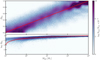 |
Fig. 1. Density maps of DEu and log DEu vs Mgal planes. With the red solid line is reported the linear relation between the average value of DEu as a function of the proto-galaxy mass. With the blue dots, we report 104 random extractions of DEu. We recall that at given Mgal the values of DEu are distributed with a triangular distribution. |
3.6. Delay times of NSMs
In this work, we used power-law DTD functions defined as follows (see Cavallo et al. 2021):
 (11)
(11)
where  is the minimum coalescence time (in this work will be always set to 1 Myr), and Ax is the normalisation constant. We choose a maximum delay time of 10 Gyr that not include all the coalescence timescales of NS-NS systems derived in Tauris et al. (2017). In order to include them we should choose a maximum delay time equal to ∞, without a significant impact on our model’s results (it would have changed only the normalisation of the DTD).
We decide to test two different pure power-laws DTD with different slopes (∝t−1 and ∝t−1.5).
In general, the rate NSMs at a certain time t can be computed by means of the following equation:
 (12)
(12)
where ψ(t) is the SFR, f(τ) is the DTD and, tmin is the minimum coalescence timescale.
kα is the number of stars in the mass range of NS progenitors per solar mass. This parameter can be computed from the integration of the initial mass function (IMF) in the mass range of NS progenitors. In this work, we assumed that the progenitors of NS are in the mass range from 9 to 50 M⊙ (same as Matteucci et al. 2014). With this assumption and using a Salpeter (1955) IMF we get  .
.
On the other side, the parameter αNS is defined as the fraction of massive stars that generate a binary system of neutron stars that will eventually merge. The value of this parameter should be chosen in order to reproduce the present rate of NSM suggested by Abbott et al. (2021;  ). From Eq. (12), using the SFR density of Madau & Dickinson (2014) and a DTD ∝ t−1.5 we obtain that αNS between 0.0009 and 0.009. In this work, we assume αNS = 0.005 that is consistent with the error interval of the observed rate of NSM by Abbott et al. (2021), and reproduces its median value.
4. Results
In this section, we present the results of our models (summarised in Table 1), and we discuss the impact of our assumptions on the chemical evolution of Eu.
Models tested in this work.
First of all, we present the effect of the new environment on the model result (i.e. MSFR) comparing it with the result of model NSt3 contained in Cavallo et al. (2021). After that, we include the effect of inefficient enrichment of europium and a varying star-formation quenching time on models results (i.e. M10 and M11). Afterwards, we test the impact of αNS on the predicted spread of [Eu/Fe] at intermediate metallicities (i.e. HC0, HC1, and HC2), to confirm the correlation reported in Cavallo et al. (2021). Finally, we discuss a scenario where both NSMs and MRD SNe are Eu producers (MRD0 and MRD1).
In Figs. 2–6 are shown the results of our models, in the [Eu/Fe]vs[Fe/H] plane. In the plots, at [Eu/Fe] = −1.5 dex, we also report the long-living stars formed without Eu (formally [Eu/Fe] = −∞).
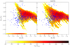 |
Fig. 2. Density plot of the distribution of simulated long-living stars predicted by our models (see the bar below the figure for the colour scale). Left panel: results of [Eu/Fe] vs [Fe/H] for model NSt3 contained in Cavallo et al. (2021). The long-living stars formed without Eu (formally [Eu/Fe] = −∞) are shown at [Eu/Fe] = −1.5 dex. The model predictions are compared to the halo stars contained in JINAbase (see Sect. 2.1) plotted with blue dots; we show as open dots the five CEMP stars discussed in Sect. 2.1. Right panel: same as left panel but for model MSFR. This model contains the modified SFRs assumed in our scenario. Note that we do not include the effects of dilution and quenching time of SF. |
 |
Fig. 3. Same as Fig. 2. Left panel: results of [Eu/Fe] vs [Fe/H] for model M10. Right panel: same as left panel but for model M11. In model M10 we included a tSF that can assume only two different values, based on the mass of the galaxy. On the other hand, model M11 assumes that the quenching time varies linearly with the galaxy mass. |
 |
Fig. 4. Results of [Eu/Fe] vs [Fe/H] for ten realisations of HC0 model. With the colour map, we show the time at which the realisation passes through a certain point in the [Eu/Fe] vs [Fe/H] plane. We also report the initial point and the time at which the first NSM exploded. With solid lines are reported the paths that each realisation follows. The path of each realisation is labelled with different colours that indicate the mass of the proto-galaxy to whom the realisation belongs. |
 |
Fig. 5. Same as Fig. 2. Left panel: results of [Eu/Fe] vs [Fe/H] for model HC0. This model is identical to model M11. We plot it again to emphasise the consequences of the variation of αNS. Central panel: same as left panel but for model HC1. In this case αNS = 0.01. To maintain constant the total amount of produced Eu, we reduce |


 |
Fig. 6. Same as Fig. 2. Left panel: results of [Eu/Fe] vs [Fe/H] for model MRD0. This model has a DTD ∝ t−1 and Eu is produced by both NSMs and MRD SNe. MRD SNe are the 10% of CC-SNe only at Z < 10−3. Right panel: same as before but for model MRD1. The model is identical to MRD0 apart from the assumed DTD (in this case ∝t−1.5). |
4.1. Impact of the new environment
To test and track the effects of the new environment on the chemical evolution of Eu we used the NSt3 model, contained in Cavallo et al. (2021), as a baseline. In the first instance, we add the hierarchical clustering scenario by computing the chemical evolution of the primordial population of proto-galaxies. Each galaxy has a star formation history described by the SFR law (see Eq. (2)). This model (MSFR) does not take into account the dilution of Eu or the quenching timescale of star formation. From Fig. 2 it is seen that the hierarchical clustering scenario assumed here, allows the model to better reproduce the observational data. In particular, with this new scenario, we can explain the presence of stars with [Eu/Fe] ∼ 0 at extremely low metallicities ([Fe/H] ∼ 3). However, this model is still not able to fit the low-metallicity tail present in the abundance distributions of halo stars.
As discussed in Sect. 3.4, this new environment adds two effects that have a great effect on the chemical evolution of Eu: (i) the motion of NS binary systems in the gravitational potential of the host galaxy can determine a merger location detached from the galaxy itself and so, only a fraction of the produced Eu is retained by the galaxy; (ii) we expect that in low mass galaxies, the SF should quench at short timescales. We implemented an Eu dilution effect that is stochastic on single NSM events but, on average, is more intense in the least massive galaxies (details in Sect. 3.5). On the other hand, for the quenching time of SF and its dependence on the mass of the galaxy, we developed two empirical relations: bi-modal and linear. To test these two effects we developed a couple of models: M10 and M11. The prescriptions of these models are identical apart from the relation used for tSF: in model M10 we assume the bi-modal behaviour of tSF and so the parameter can assume only two values, based on the mass of the galaxy; on the other side in model M11, the value tSF scales linearly with the mass of the galaxy. Parameters assumed in models M10 and M11 are reported in Table 1. In Fig. 3 are reported the results of model M10 (left panel) and model M11 (right panel). As seen in Fig. 3, both models show a good fit to the observed stars and, in particular, can explain the presence of stars with [Eu/Fe] < 0 in the extremely metal-poor environment (i.e. [Fe/H] < −3).
From now on, we will refer to M11 as our best model (of the NS-only scenario). Even if M11 and M10 produce similar results, M11 assumes a tSF vs Mgal relation more realistic than the one assumed in M10 (linear against bi-modal).
To have a better comprehension of the impact of the hierarchical clustering framework, now we will describe how our stochastic chemical evolution model works. As we introduced in Sect. 3, the stochastic model consists of ∼200 realisations in which we compute the chemical evolution. In this work, each realisation is associated with one galaxy in our population (note that a single galaxy can be linked to more than one stochastic realisation, depending on its mass). So, with this construction, at each time-step, we can study the chemical composition of a single realisation and, therefore, trace its time evolution. In Fig. 4 are plotted ten realisations of model HC0 (identical to model M11) on the [Eu/Fe] vs [Fe/H] plane. The path of each realisation through the [Eu/Fe] vs [Fe/H] plane is colour coded with a colour map that shows the time at which the realisation passes a certain point in the plane. In the figure are also reported the initial point (with coloured diamonds) and the time (in Myr) at which the first NSM has exploded. Moreover, starting points, epochs of the first NSM event, and paths of single realisations are labelled with different colours, based on the mass of the galaxy linked to them. In the following some important features of the model, that can be inferred by Fig. 4, will be discussed.
-
In our model, the star formation is stochastic and so it is the formation of binary systems of NS. For this reason, we can have realisations where the first NSM explode at ∼90 Myr, but also realisation where this happened later at ∼160 Myr. Regarding the time of the first NSM explosion, we can also identify a clear trend: in the least massive galaxies, the first NSM appear later than in most massive ones. In fact looking at Fig. 4, is seen that in low mass galaxies (with 105 ≤ Mgal ≤ 106 M⊙; labelled in blue) the first NSM occurs, on average, at ∼125 Myr; on the other side, in the most massive galaxies (with 108 < Mgal ≤ 109 M⊙; labelled in red) the fist NSM explode at ∼95 Myr. This trend is a direct effect of the fact low mass galaxies transform less mass of gas into stars at each time-step (i.e. lower star formation efficiency; see Eq. (3)) compared to the most massive ones. However, also in realisations that belong to galaxies of the same mass class, we can notice variability in the epoch of the first NSM explosion. This is caused by the fact that SF is stochastic.
-
The trace of each realisation starts with a different value of [Eu/Fe] at different metallicities. Also, in this case, it is possible to identify a trend: galaxies of low mass (labelled in blue) enter into the plane at lower [Eu/Fe] compared to the “red” (plotted in red) ones: the dilution effect is stronger in galaxies with lower masses and therefore the ratio [Eu/Fe] is lower.
-
The realisations follow different paths in the [Eu/Fe] vs [Fe/H] plane. Into these paths, is possible to notice some patterns, which can be understood in terms of the enrichment that takes place in that volume. For example, when a realisation moves horizontally (at constant [Eu/Fe]) towards lower metallicities, no events are enriching the ISM in iron and europium, and the gas is diluted by the in-falling gas with primordial composition. Then, when an event produces Fe, the realisation moves to higher metallicities and lower [Eu/Fe] ratios. If a NSM explodes, the realisation makes a “jump” towards higher [Eu/Fe] values. The height of these “jumps” varies among different realisations due to the combination of two facts: (i) the amount of Eu that a single NSM can produce is variable (as Eq. (7)). (ii) the fraction of Eu retained by the host galaxy varies from one NSM to another (see Fig. 1).
In our scenario, least massive galaxies could not produce stars with [Eu/Fe] > 1. However, r-II stars (highly enhanced r-process elements stars with [Eu/Fe] > 0.7) have been observed in Reticulum II, an ultra-faint dwarf galaxy (Ji et al. 2016; Roederer et al. 2016). In our scenario, where the enrichment in dwarf galaxies is strongly diluted, galaxies like Reticulum II could not be enriched by NSMs but by a secondary source(s) of Eu (e.g. MRD and/or CC SNe).
Other works, such as Brauer et al. (2019), Hattori et al. (2023), and Hirai et al. (2022), found that (at least a fraction) of metal-poor r-II stars in the Galactic halo formed in ancient ultra-faint dwarf (UFD) galaxies (similar to Reticulum II). With our model, we can recover those conclusions by assuming a different probability distribution for DEu (see Fig. 1). In this work, we implement the inefficient enrichment of Eu in low-mass galaxies following the prescriptions of Bonetti et al. (2019).
That model predicts that the Eu enrichment in galaxies similar to Reticulum II is rare and not enough robust to explain the observations of Reticulum II. However is still possible that, with Reticulum II, we detect a rare member of a large population of poorly enriched UFD galaxies. Future observations of r-II stars in several UFD would certainly help to solve the tension with the picture that we adopt.
4.2. Effects of αNS
As we introduced in previous sections, the shape of the DTD has a great impact on the chemical evolution of Eu. Another parameter, that is linked with the DTD by definition is the fraction of massive stars that are in a binary system with the right characteristics to lead to a NSM: αNS. This parameter can be calculated, given the DTD, SFR, and the mass range of NS progenitors, imposing that the theoretical rate of NSM at the present time (see Eq. (12)) is consistent with the observed one. For the DTDs used in this paper, previous works suggest a wide range of αNS, from 1 − 2 × 10⁻² (Giacobbo & Mapelli 2018; Simonetti et al. 2019; Greggio et al. 2021) up to 5 − 6 × 10⁻² (Molero et al. 2021). More recent estimates of the value of the present rate of NSM (e.g. Abbott et al. 2021) point to αNS < 0.01. The uncertainty of αNS values is correlated with the large error bars in the rate of NSM observed at the present day calculated and revised by Abbott et al. (2017a, 2020, 2021).
Giacobbo & Mapelli (2018), with a binary population synthesis model, suggest that the formation of binary systems of NS is influenced by the environment metallicity. This can be parametrized by assuming a dependence of αNS on [Fe/H]. Moreover, this dependency has a weak influence on the predicted present rate of NSM, as shown by Simonetti et al. (2019). However, no strong observational evidence has been found to support this dependency.
In Cavallo et al. (2021), we presented the correlation between the dispersion of the [Eu/Fe] values and the fraction of massive stars that can generate a NSM (αNS). In particular, the spread shrinks when we assume higher αNS values.
For these reasons, we decide to test the dependence of [Eu/Fe] dispersion on αNS with three models: HC0, HC1, and HC2 (see Table 1). These models assume different values for αNS and, as a consequence, for  : 0.005 (HC0), 0.01 (HC1), and 0.02 (HC2); results of these models are plotted in Fig. 5, where is possible to see the correlation cited above.
Focusing on intermediate metallicities ([Fe/H] > −2.5) is possible to notice the impact of αNS on the predicted spread (see Cavallo et al. 2021). In this metallicity range is possible to check whether or not models with a certain αNS are able to reproduce the spread observed in halo stars. Thus, our model seems to be a promising tool that allows us to estimate the αNS parameter and, as a consequence,  . However, since the current data of Eu abundances of halo stars are affected by large uncertainties (∼0.2 − 0.3 dex), we cannot reject any of the tested models. Future surveys such as 4MOST (de Jong et al. 2014) and WEAVE (Dalton et al. 2012) will produce larger and more precise data-sets so to allow us to determine the value of αNS more precisely.
4.3. Eu production from MRD SNe
As we already mentioned, lots of studies on the nucleosynthesis of r-process elements indicate NSMs as a promising r-process site (Freiburghaus et al. 1999; Korobkin et al. 2012; Wanajo et al. 2014; Radice et al. 2018). However, as we point out in Cavallo et al. (2021), in our stochastic chemical evolution model NSM with a DTD ∝ t−1 are not able to reproduce the abundances distribution of halo stars. In this section, we want to test what are the effects of adding a second source of Eu to the NSM with a DTD ∝ t−1 (and ∝ t−1.5). However, CC SNe seems to be ruled out as a major producer of Eu, as suggested by nucleosynthesis models (Arcones et al. 2007; Arcones & Thielemann 2013; Wanajo et al. 2018). On the other hand, particular classes of CC SNe could potentially be a source of r-process elements. The major proposed candidates are collapsars (Siegel et al. 2019) and MRD SNe (Winteler et al. 2012; Nishimura et al. 2015; Reichert et al. 2020). Note that in these models tSF is equal to 1 Gyr for all the proto-galaxies.
We decide to test the scenario where both NSMs and MRD SNe (active only at Z < 10−3) produce Eu in this new framework. We develop two different models that differ only on the assumed DTD: MRD0 (DTD ∝ t−1) and MRD1 (DTD ∝ t−1.5); in Fig. 6 are plotted the results of these models.
Looking at the right panel of Fig. 6, is seen that with the addition of the second source of Eu (in this case MRD-SNe) the model is able to explain both the large [Eu/Fe] spread at [Fe/H] ≤ −2.5 and the mean trend of [Eu/Fe] vs [Fe/H] at high metallicity ([Fe/H] > −2) without assumptions on the tSF of the proto-galaxies.
In the left panel of Fig. 6 it can also be noticed that the mixed scenario is not able to reproduce the wide spread of the data when we assume DTD ∝ t−1 for the NSMs. In particular, the model fails to explain the presence of stars with [Eu/Fe] > 1.5 and also the trend of [Eu/Fe] at higher metalicities.
We note that all our models fail to explain the group of ∼6 Eu-enhanced stars at [Fe/H] > −2.5 present in our observational sample. As discussed in Sect. 2.1 five of them are CEMP stars that are not the main focus of this work. On the other hand, our models fail to explain the presence of the ordinary star with [Eu/Fe] ∼ 1.7 at [Fe/H] ∼ −2.1. Further studies on the chemical composition of SMSS J175046.30−425506.9 could provide clues on its origin.
4.4. Eu-free stars
As underlined in previous versions of this model (Cescutti et al. 2015; Cavallo et al. 2021), our stochastic chemical evolution model predicts the presence of Eu-free stars (i.e. [Eu/Fe] = −∞). This is due to the fact that only a small fraction of stars pollutes the ISM with r-process elements (compared to the number of SNe II). So at extremely low metallicities ([Fe/H] < −3), some stars could have been born in regions where the gas is Eu-free (not polluted from r-process events). In particular, models with lower values of αNS should predict a high number of Eu-free stars. Moreover, models that assume longer delay times for NSM will produce higher fractions of Eu-free stars, at higher metallicities. In this section, we will compare the fraction of Eu-free stars predicted by our models and the observational constraints on its value.
The model prediction of the fraction of Eu-free stars is computed as the ratio of stars without Eu over the total number of stars in our model in a given metallicity bin. To calculate the observational ratio, we take all the halo stars for which Ba has been observed contained in JINAbase2. The number of this stars which have only an upper limit measurement of Eu over the total number of them, in a given [Fe/H] bin, is our observational proxy of Eu-free stars. Indeed, the fact that we can observe barium, but no europium could be a sign of the absence of europium in these stars; however, in most cases, it is probably an observational problem due to the weakness of europium lines compared to barium lines. Still, we can use this observational proxy as upper limits useful in providing constraints to the models.
In Fig. 7 is plotted the comparison between predicted and observed ratios of Eu-free stars as a function of [Fe/H]. Looking at Fig. 7 (left panel), is seen that models M10 and M11 predict similar fractions of Eu-free stars at fixed [Fe/He]. Moreover, is possible to appreciate the overall reduction of predicted Eu-free stars compared to model NSt3 (orange line) presented in our last work. This reduction is caused by the change of environment, in particular, by the inefficiency in the Eu enrichment (especially in the least massive galaxies). In this case, especially at low metallicities ([Fe/H] < −3) the predicted fraction of Eu-free stars is above the observed ones; those are upper limits. The fact that models M10 and M11 produce too many stars formed without Eu, can be explained by the characteristic time scale of the Eu enrichment by NSMs (on average, longer than the one associated with massive stars).
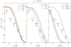 |
Fig. 7. Comparison between the predicted and observed ratios of Eu-free stars over the total number of stars for bins of 0.5 dex in [Fe/H]. Blue and red markers are the observational proxies for the ratio; so the ratio between the number of stars for which Eu only presents an upper limit (possibly Eu-free) over the number of stars with measured Ba. Observational ratios derived from the JINAbase data-set Abohalima & Frebel (2018) are plotted in red. Left panel: ratio of Eu-free stars for model MSFR, M10, M11 (in black), and NSt3 from Cavallo et al. (2021; in orange). Central panel: same as left panel but for models HC0, HC1, and HC2. Right panel: same as left panel but for model MRD0, MRD1 (in black), and HC0 (in green). |
In the central panel of Fig. 7 is possible to appreciate the correlation between the value of the parameter (αNS) and the fraction of Eu-free stars predicted. In particular, a model with higher αNS (i.e. NSMs are less rare at all the metallicities) predicts a lower fraction of Eu-free stars. Similar to the previous case, the predictions of our models are not compatible with the chosen observational proxies, for the same reason reported above.
In the last panel are plotted the results of models where both NSM and MRD SNe are Eu producers and their comparison with the ones of HC0. From this panel, we can observe two different things: (a) models where the MRD SNe channel is active predicts a lower fraction of Eu-free stars, due to the early contribution of massive stars to the Eu enrichment (black lines vs green one); (b) models with a steeper DTD (i.e. shorter delay times for NSMs) produce a lower amount of Eu-free stars, due to the shorter time between the formation of the NS binary system and the merging event. It is also important to underline that the predicted fractions of Eu-free stars are compatible or lower than the observed ones.
As discussed in the introduction, Eu is the perfect tracer of r-process because is mainly produced by this neutron-capture channel. So, what we define Eu free stars are stars without europium produced by an r-process. On the other side, we cannot exclude that other neutron capture channels may produce europium at this metallicity. For example, the s-process in rotating massive stars (see Frischknecht et al. 2016; Limongi & Chieffi 2018) could produce a tiny amount of europium. From this channel, the Eu enrichment at [Fe/H] ∼ −3 is expected to be very low with a [Eu/Fe] < −4 (at least two orders of magnitude less than NSMs) with an [Eu/H] < −7. However, given the weakness of the europium line, this pollution is likely impossible to be detected in stellar spectra at least with present spectroscopic capabilities.
5. Conclusions
In this work, we use the stochastic chemical evolution model of the Galactic halo presented by Cescutti et al. (2006) and updated by Cescutti et al. (2015). We aim at reproducing the large spread in the [Eu/Fe] ratio observed in Galactic halo stars and solve the tensions noted in our previous work (Cavallo et al. 2021). In particular, we assume that the Galactic halo has been formed by the accretion of a population of (∼100) proto-galaxies with mass from 105 to 109 M⊙. We compute the chemical evolution of Eu in these proto-galaxies, which is influenced by two effects: (i) the lower increase of the Eu abundance caused by the dynamics of NS binary systems which can easily escape from the gravitational potential of the host galaxy (see Bonetti et al. 2019), and (ii) SF timescales shorter in low mass galaxies due to the low binding energy of the gas inside the proto-galaxy. These effects depend on the mass of the proto-galaxy that we are considering. Therefore, we introduce relations that depend on the mass of the proto-galaxy for both these effects. In particular, for the dilution of Eu, we also add event-to-event stochasticity. We decide to take model NSt3 from Cavallo et al. (2021) and we add the effects mentioned above. In models where NSM are the sole producers of Eu we assume that these systems follow a delay time distribution (DTD) ∝t−1.5 with a minimum coalescence time of 1 Myr. For NSMs Eu yields, we followed the prescriptions of Matteucci et al. (2014) and Cescutti et al. (2015). We also tested the scenario where both NSMs and MRD SNe (a particular class of CC SNe) produce Eu.
Our main conclusions can be summarised as follows:
-
If we assume that NSMs are the sole producers of Eu, the hierarchical formation of the Galactic halo, combined with the inefficient enrichment of Eu in low mass proto-galaxies, can explain the presence of extremely metal-poor stars (i.e. [Fe/H] ≤ −3) that present sub-solar [Eu/Fe] ratios. In this framework, the coalescence timescale of binary systems of neutron stars should follow a DTD ∝ t−1.5, each NSM event produces an average of 1.6 × 10⁻⁵ M⊙ of Eu, αNS is fixed at 0.005, and progenitors of NS should be in the mass range from 9 to 50 M⊙.
-
Adopting our best model (M11/HC0) we confirm the correlation, studied in our previous work (see Cavallo et al. 2021), between αNS and the dispersion of [Eu/Fe] at a given metallicity, and reach similar conclusions: present literature data cannot allow us to put strong constraints of αNS. However, future high-resolution spectroscopical surveys, such as 4MOST (de Jong et al. 2014) and WEAVE (Dalton et al. 2012), will produce the necessary statistic to constrain at best this parameter.
-
NSMs with a DTD ∝ t−1 are not able to explain the large star-to-star scatter of [Eu/Fe] observed in the Galactic halo, also in the mixed scenario in which both NSMs and MRD SNe produce Eu. However, this scenario is in agreement with observational data when we assume a DTD for NSMs ∝t−1.5.
-
The fractions of Eu-free stars of models in which we assume that Eu is only produced by the NSMs cannot be reconciled with observations. This is a potential issue for the concept of r-process produced exclusively by NSMs. On the other hand, when we add the second source of Eu (i.e. the MRD SNe) the models predict ratios of Eu-free stars in agreement with observations. In particular, these ratios are below or comparable to the observational values but that is not an issue. We know that a potentially large number of these observed Eu-free stars are most likely to be false Eu-free stars, and so the observational values should be considered as upper limits. Furthermore, the value of Eu-free stars cannot be clearly evaluated and no firm conclusions can be drawn.
Finally, we accomplished our initial goal: solve the tension noted in our previous work. In order to do that, we included our chemical evolution model in the hierarchical scenario and we also took into account the effects on chemical evolution produced by the environment of small proto-galaxies.
In future work, we aim at reproducing the solar abundances and present-day NSMs rate with a new version of this model able to mimic the Galactic disk environment.
Formally the effect dilutes [Eu/Fe]. From this point when we talk about “Eu dilution” we are referring to the dilution of [Eu/Fe].
Selected stars are contained in: Ryan et al. (1991, 1996), McWilliam et al. (1995), Norris et al. (1997), Burris et al. (2000), Fulbright (2000), Preston & Sneden (2000, 2001), Westin et al. (2000), Aoki et al. (2002b, 2005, 2007a,b), 2008, 2012, 2013, 2014), Carretta et al. (2002), Cowan et al. (2002), Johnson (2002), Lucatello et al. (2003), Ivans et al. (2003), Ivans et al. (2006), Sneden et al. (2003), Cayrel et al. (2004), Christlieb et al. (2004), Cohen et al. (2004, 2008, 2013), Honda et al. (2004, 2011), Johnson & Bolte (2004), Barbuy et al. (2005), Barklem et al. (2005), Jonsell et al. (2005, 2006), Masseron et al. (2006, 2012), Preston et al. (2006), Sivarani et al. (2006), Frebel et al. (2007), Lai et al. (2007, 2008), Roederer et al. (2008, 2010, 2014), Bonifacio et al. (2009), Hayek et al. (2009), Zhang et al. (2009), Behara et al. (2010), Ishigaki et al. (2010, 2013), Bensby et al. (2011), Caffau et al. (2011), Hansen et al. (2011, 2012, 2015), Allen et al. (2012), Cui et al. (2013), Placco et al. (2013, 2014), Yong et al. (2013), Mashonkina et al. (2014), Siqueira Mello et al. (2014), Spite et al. (2014), Jacobson et al. (2015), Li et al. (2015b).
Acknowledgments
We thank an anonymous referee for his/her comments which improved the quality of this paper. L.C. thanks Matteo Bonetti for useful discussions on the core part of this work. This work was partially supported by the European Union (ChETEC-INFRA, project no. 101008324).
References
- Abbott, B. P., Abbott, R., Abbott, T. D., et al. 2017a, Phys. Rev. Lett., 119, 161101 [Google Scholar]
- Abbott, B. P., Abbott, R., Abbott, T. D., et al. 2017b, ApJ, 848, L13 [CrossRef] [Google Scholar]
- Abbott, B. P., Abbott, R., Abbott, T. D., et al. 2017c, Phys. Rev. D, 95, 082005 [NASA ADS] [CrossRef] [Google Scholar]
- Abbott, B. P., Abbott, R., Abbott, T. D., et al. 2020, ApJ, 892, L3 [NASA ADS] [CrossRef] [Google Scholar]
- Abbott, R., Abbott, T. D., Abraham, S., et al. 2021, ApJ, 913, L7 [NASA ADS] [CrossRef] [Google Scholar]
- Abohalima, A., & Frebel, A. 2018, ApJS, 238, 36 [NASA ADS] [CrossRef] [Google Scholar]
- Aguado, D. S., Myeong, G. C., Belokurov, V., et al. 2021, MNRAS, 500, 889 [NASA ADS] [Google Scholar]
- Allen, D. M., Ryan, S. G., Rossi, S., Beers, T. C., & Tsangarides, S. A. 2012, A&A, 548, A34 [NASA ADS] [CrossRef] [EDP Sciences] [Google Scholar]
- Aoki, W., Norris, J. E., Ryan, S. G., Beers, T. C., & Ando, H. 2002a, PASJ, 54, 933 [NASA ADS] [CrossRef] [Google Scholar]
- Aoki, W., Ando, H., Honda, S., et al. 2002b, PASJ, 54, 427 [NASA ADS] [Google Scholar]
- Aoki, W., Honda, S., Beers, T. C., et al. 2005, ApJ, 632, 611 [NASA ADS] [CrossRef] [Google Scholar]
- Aoki, W., Beers, T. C., Christlieb, N., et al. 2007a, ApJ, 655, 492 [NASA ADS] [CrossRef] [Google Scholar]
- Aoki, W., Honda, S., Sadakane, K., & Arimoto, N. 2007b, PASJ, 59, L15 [NASA ADS] [Google Scholar]
- Aoki, W., Beers, T. C., Sivarani, T., et al. 2008, ApJ, 678, 1351 [Google Scholar]
- Aoki, W., Ito, H., & Tajitsu, A. 2012, ApJ, 751, L6 [NASA ADS] [CrossRef] [Google Scholar]
- Aoki, W., Beers, T. C., Lee, Y. S., et al. 2013, AJ, 145, 13 [CrossRef] [Google Scholar]
- Aoki, W., Tominaga, N., Beers, T. C., Honda, S., & Lee, Y. S. 2014, Science, 345, 912 [NASA ADS] [CrossRef] [Google Scholar]
- Arcones, A., & Thielemann, F. K. 2013, J. Phys. G Nucl. Phys., 40, 013201 [NASA ADS] [CrossRef] [Google Scholar]
- Arcones, A., Janka, H. T., & Scheck, L. 2007, A&A, 467, 1227 [CrossRef] [EDP Sciences] [Google Scholar]
- Argast, D., Samland, M., Thielemann, F. K., & Qian, Y. Z. 2004, A&A, 416, 997 [NASA ADS] [CrossRef] [EDP Sciences] [Google Scholar]
- Barbuy, B., Spite, M., Spite, F., et al. 2005, A&A, 429, 1031 [NASA ADS] [CrossRef] [EDP Sciences] [Google Scholar]
- Barklem, P. S., Christlieb, N., Beers, T. C., et al. 2005, A&A, 439, 129 [NASA ADS] [CrossRef] [EDP Sciences] [Google Scholar]
- Bauswein, A., Goriely, S., & Janka, H. T. 2013, ApJ, 773, 78 [NASA ADS] [CrossRef] [Google Scholar]
- Behara, N. T., Bonifacio, P., Ludwig, H. G., et al. 2010, A&A, 513, A72 [NASA ADS] [CrossRef] [EDP Sciences] [Google Scholar]
- Belczynski, K., Klencki, J., Fields, C. E., et al. 2020, A&A, 636, A104 [NASA ADS] [CrossRef] [EDP Sciences] [Google Scholar]
- Belokurov, V., Zucker, D. B., Evans, N. W., et al. 2006, ApJ, 642, L137 [Google Scholar]
- Belokurov, V., Erkal, D., Evans, N. W., Koposov, S. E., & Deason, A. J. 2018, MNRAS, 478, 611 [Google Scholar]
- Bensby, T., Adén, D., Meléndez, J., et al. 2011, A&A, 533, A134 [NASA ADS] [CrossRef] [EDP Sciences] [Google Scholar]
- Berger, E. 2014, ARA&A, 52, 43 [CrossRef] [Google Scholar]
- Bisterzo, S., Gallino, R., Käppeler, F., et al. 2015, MNRAS, 449, 506 [Google Scholar]
- Bonetti, M., Perego, A., Dotti, M., & Cescutti, G. 2019, MNRAS, 490, 296 [NASA ADS] [CrossRef] [Google Scholar]
- Bonifacio, P., Spite, M., Cayrel, R., et al. 2009, A&A, 501, 519 [NASA ADS] [CrossRef] [EDP Sciences] [Google Scholar]
- Bonifacio, P., Sbordone, L., Caffau, E., et al. 2012, A&A, 542, A87 [NASA ADS] [CrossRef] [EDP Sciences] [Google Scholar]
- Brauer, K., Ji, A. P., Frebel, A., et al. 2019, ApJ, 871, 247 [NASA ADS] [CrossRef] [Google Scholar]
- Bullock, J. S., & Johnston, K. V. 2005, ApJ, 635, 931 [Google Scholar]
- Burris, D. L., Pilachowski, C. A., Armandroff, T. E., et al. 2000, ApJ, 544, 302 [Google Scholar]
- Caffau, E., Bonifacio, P., François, P., et al. 2011, A&A, 534, A4 [NASA ADS] [CrossRef] [EDP Sciences] [Google Scholar]
- Calura, F., Lanfranchi, G. A., & Matteucci, F. 2008, A&A, 484, 107 [NASA ADS] [CrossRef] [EDP Sciences] [Google Scholar]
- Cameron, A. 1982, Essays in Nuclear Astrophysics (Cambridge: Cambridge University Press), 23 [Google Scholar]
- Carretta, E., Gratton, R., Cohen, J. G., Beers, T. C., & Christlieb, N. 2002, AJ, 124, 481 [NASA ADS] [CrossRef] [Google Scholar]
- Cavallo, L., Cescutti, G., & Matteucci, F. 2021, MNRAS, 503, 1 [CrossRef] [Google Scholar]
- Cayrel, R., Depagne, E., Spite, M., et al. 2004, A&A, 416, 1117 [NASA ADS] [CrossRef] [EDP Sciences] [Google Scholar]
- Cescutti, G. 2008, A&A, 481, 691 [NASA ADS] [CrossRef] [EDP Sciences] [Google Scholar]
- Cescutti, G., François, P., Matteucci, F., Cayrel, R., & Spite, M. 2006, A&A, 448, 557 [NASA ADS] [CrossRef] [EDP Sciences] [Google Scholar]
- Cescutti, G., Romano, D., Matteucci, F., Chiappini, C., & Hirschi, R. 2015, A&A, 577, A139 [NASA ADS] [CrossRef] [EDP Sciences] [Google Scholar]
- Chiappini, C., Ekström, S., Meynet, G., et al. 2008, A&A, 479, L9 [NASA ADS] [CrossRef] [EDP Sciences] [Google Scholar]
- Christlieb, N., Gustafsson, B., Korn, A. J., et al. 2004, ApJ, 603, 708 [NASA ADS] [CrossRef] [Google Scholar]
- Chruslinska, M., Belczynski, K., Klencki, J., & Benacquista, M. 2018, MNRAS, 474, 2937 [CrossRef] [Google Scholar]
- Ciolfi, R. 2020, Front. Astron. Space Sci., 7, 27 [NASA ADS] [CrossRef] [Google Scholar]
- Cohen, J. G., Christlieb, N., McWilliam, A., et al. 2004, ApJ, 612, 1107 [CrossRef] [Google Scholar]
- Cohen, J. G., Christlieb, N., McWilliam, A., et al. 2008, ApJ, 672, 320 [NASA ADS] [CrossRef] [Google Scholar]
- Cohen, J. G., Christlieb, N., Thompson, I., et al. 2013, ApJ, 778, 56 [Google Scholar]
- Cooper, A. P., Cole, S., Frenk, C. S., et al. 2010, MNRAS, 406, 744 [Google Scholar]
- Côté, B., Eichler, M., Arcones, A., et al. 2019, ApJ, 875, 106 [Google Scholar]
- Coulter, D. A., Foley, R. J., Kilpatrick, C. D., et al. 2017, Science, 358, 1556 [NASA ADS] [CrossRef] [Google Scholar]
- Cowan, J. J., Thielemann, F.-K., & Truran, J. W. 1991, Phys. Rep., 208, 267 [NASA ADS] [CrossRef] [Google Scholar]
- Cowan, J. J., Sneden, C., Burles, S., et al. 2002, ApJ, 572, 861 [NASA ADS] [CrossRef] [Google Scholar]
- Cowperthwaite, P. S., Berger, E., Villar, V. A., et al. 2017, ApJ, 848, L17 [CrossRef] [Google Scholar]
- Cui, W. Y., Sivarani, T., & Christlieb, N. 2013, A&A, 558, A36 [NASA ADS] [CrossRef] [EDP Sciences] [Google Scholar]
- Curtis, S., Ebinger, K., Fröhlich, C., et al. 2019, ApJ, 870, 2 [Google Scholar]
- Dalton, G., Trager, S. C., Abrams, D. C., et al. 2012, SPIE Conf. Ser., 8446, 84460P [Google Scholar]
- D’Avanzo, P. 2015, J. High Energy Astrophys., 7, 73 [CrossRef] [Google Scholar]
- D’Avanzo, P., Salvaterra, R., Bernardini, M. G., et al. 2014, MNRAS, 442, 2342 [Google Scholar]
- de Jong, R. S., Barden, S., Bellido-Tirado, O., et al. 2014, SPIE Conf. Ser., 9147, 91470M [NASA ADS] [Google Scholar]
- Dominik, M., Belczynski, K., Fryer, C., et al. 2012, ApJ, 759, 52 [Google Scholar]
- Eichler, D., Livio, M., Piran, T., & Schramm, D. N. 1989, Nature, 340, 126 [NASA ADS] [CrossRef] [Google Scholar]
- Fattahi, A., Belokurov, V., Deason, A. J., et al. 2019, MNRAS, 484, 4471 [NASA ADS] [CrossRef] [Google Scholar]
- Fattahi, A., Deason, A. J., Frenk, C. S., et al. 2020, MNRAS, 497, 4459 [NASA ADS] [CrossRef] [Google Scholar]
- Fong, W., Berger, E., Blanchard, P. K., et al. 2017, ApJ, 848, L23 [NASA ADS] [CrossRef] [Google Scholar]
- Frebel, A., Christlieb, N., Norris, J. E., et al. 2007, ApJ, 660, L117 [NASA ADS] [CrossRef] [Google Scholar]
- Frebel, A., Kirby, E. N., & Simon, J. D. 2010, Nature, 464, 72 [NASA ADS] [CrossRef] [Google Scholar]
- Freiburghaus, C., Rosswog, S., & Thielemann, F. K. 1999, ApJ, 525, L121 [NASA ADS] [CrossRef] [Google Scholar]
- Frischknecht, U., Hirschi, R., Pignatari, M., et al. 2016, MNRAS, 456, 1803 [Google Scholar]
- Fruchter, A. S., Levan, A. J., Strolger, L., et al. 2006, Nature, 441, 463 [NASA ADS] [CrossRef] [Google Scholar]
- Fulbright, J. P. 2000, AJ, 120, 1841 [NASA ADS] [CrossRef] [Google Scholar]
- Gaia Collaboration (Brown, A. G. A., et al.) 2016, A&A, 595, A2 [NASA ADS] [CrossRef] [EDP Sciences] [Google Scholar]
- Gaia Collaboration (Brown, A. G. A., et al.) 2018, A&A, 616, A1 [NASA ADS] [CrossRef] [EDP Sciences] [Google Scholar]
- Ghirlanda, G., Salafia, O. S., Pescalli, A., et al. 2016, A&A, 594, A84 [NASA ADS] [CrossRef] [EDP Sciences] [Google Scholar]
- Giacobbo, N., & Mapelli, M. 2018, MNRAS, 480, 2011 [Google Scholar]
- Giacobbo, N., & Mapelli, M. 2019, MNRAS, 482, 2234 [Google Scholar]
- Goldstein, A., Veres, P., Burns, E., et al. 2017, ApJ, 848, L14 [CrossRef] [Google Scholar]
- Graur, O., Poznanski, D., Maoz, D., et al. 2011, MNRAS, 417, 916 [Google Scholar]
- Greggio, L. 2005, A&A, 441, 1055 [NASA ADS] [CrossRef] [EDP Sciences] [Google Scholar]
- Greggio, L., Simonetti, P., & Matteucci, F. 2021, MNRAS, 500, 1755 [Google Scholar]
- Guetta, D., & Piran, T. 2006, A&A, 453, 823 [NASA ADS] [CrossRef] [EDP Sciences] [Google Scholar]
- Hansen, C. J., Nordström, B., Bonifacio, P., et al. 2011, A&A, 527, A65 [NASA ADS] [CrossRef] [EDP Sciences] [Google Scholar]
- Hansen, C. J., Primas, F., Hartman, H., et al. 2012, A&A, 545, A31 [NASA ADS] [CrossRef] [EDP Sciences] [Google Scholar]
- Hansen, T., Hansen, C. J., Christlieb, N., et al. 2015, ApJ, 807, 173 [Google Scholar]
- Hattori, K., Okuno, A., & Roederer, I. U. 2023, ApJ, 946, 48 [NASA ADS] [CrossRef] [Google Scholar]
- Hayek, W., Wiesendahl, U., Christlieb, N., et al. 2009, A&A, 504, 511 [NASA ADS] [CrossRef] [EDP Sciences] [Google Scholar]
- Helmi, A., Babusiaux, C., Koppelman, H. H., et al. 2018, Nature, 563, 85 [Google Scholar]
- Heringer, E., Pritchet, C., Kezwer, J., et al. 2017, ApJ, 834, 15 [Google Scholar]
- Hirai, Y., Ishimaru, Y., Saitoh, T. R., et al. 2015, ApJ, 814, 41 [NASA ADS] [CrossRef] [Google Scholar]
- Hirai, Y., Beers, T. C., Chiba, M., et al. 2022, MNRAS, 517, 4856 [NASA ADS] [CrossRef] [Google Scholar]
- Hollek, J. K., Frebel, A., Roederer, I. U., et al. 2011, ApJ, 742, 54 [NASA ADS] [CrossRef] [Google Scholar]
- Honda, S., Aoki, W., Kajino, T., et al. 2004, ApJ, 607, 474 [NASA ADS] [CrossRef] [Google Scholar]
- Honda, S., Aoki, W., Beers, T. C., & Takada-Hidai, M. 2011, ApJ, 730, 77 [NASA ADS] [CrossRef] [Google Scholar]
- Hotokezaka, K., Kiuchi, K., Kyutoku, K., et al. 2013, Phys. Rev. D, 88, 044026 [Google Scholar]
- Howard, W. M., Arnett, W. D., Clayton, D. D., & Woosley, S. E. 1972, ApJ, 175, 201 [NASA ADS] [CrossRef] [Google Scholar]
- Howard, W. M., Mathews, G. J., Takahashi, K., & Ward, R. A. 1986, ApJ, 309, 633 [NASA ADS] [CrossRef] [Google Scholar]
- Ishigaki, M., Chiba, M., & Aoki, W. 2010, PASJ, 62, 143 [NASA ADS] [Google Scholar]
- Ishigaki, M. N., Aoki, W., & Chiba, M. 2013, ApJ, 771, 67 [NASA ADS] [CrossRef] [Google Scholar]
- Ishimaru, Y., Wanajo, S., & Prantzos, N. 2015, ApJ, 804, L35 [NASA ADS] [CrossRef] [Google Scholar]
- Ivans, I. I., Sneden, C., James, C. R., et al. 2003, ApJ, 592, 906 [NASA ADS] [CrossRef] [Google Scholar]
- Ivans, I. I., Simmerer, J., Sneden, C., et al. 2006, ApJ, 645, 613 [NASA ADS] [CrossRef] [Google Scholar]
- Ivezić, Ž., Beers, T. C., & Jurić, M. 2012, ARA&A, 50, 251 [Google Scholar]
- Jacobson, H. R., Keller, S., Frebel, A., et al. 2015, ApJ, 807, 171 [NASA ADS] [CrossRef] [Google Scholar]
- Ji, A. P., Frebel, A., Chiti, A., & Simon, J. D. 2016, Nature, 531, 610 [NASA ADS] [CrossRef] [Google Scholar]
- Johnson, J. A. 2002, ApJS, 139, 219 [Google Scholar]
- Johnson, J. A., & Bolte, M. 2004, ApJ, 605, 462 [Google Scholar]
- Johnston, K. V., Bullock, J. S., Sharma, S., et al. 2008, ApJ, 689, 936 [Google Scholar]
- Jonsell, K., Edvardsson, B., Gustafsson, B., et al. 2005, A&A, 440, 321 [NASA ADS] [CrossRef] [EDP Sciences] [Google Scholar]
- Jonsell, K., Barklem, P. S., Gustafsson, B., et al. 2006, A&A, 451, 651 [NASA ADS] [CrossRef] [EDP Sciences] [Google Scholar]
- Kirby, E. N., Cohen, J. G., Guhathakurta, P., et al. 2013, ApJ, 779, 102 [Google Scholar]
- Koch, A., & Edvardsson, B. 2002, A&A, 381, 500 [NASA ADS] [CrossRef] [EDP Sciences] [Google Scholar]
- Komiya, Y., & Shigeyama, T. 2016, ApJ, 830, 76 [NASA ADS] [CrossRef] [Google Scholar]
- Korobkin, O., Rosswog, S., Arcones, A., & Winteler, C. 2012, MNRAS, 426, 1940 [NASA ADS] [CrossRef] [Google Scholar]
- Krisciunas, K., Contreras, C., Burns, C. R., et al. 2017, AJ, 154, 211 [NASA ADS] [CrossRef] [Google Scholar]
- Lai, D. K., Johnson, J. A., Bolte, M., & Lucatello, S. 2007, ApJ, 667, 1185 [Google Scholar]
- Lai, D. K., Bolte, M., Johnson, J. A., et al. 2008, ApJ, 681, 1524 [NASA ADS] [CrossRef] [Google Scholar]
- Lanfranchi, G. A., & Matteucci, F. 2003, MNRAS, 345, 71 [Google Scholar]
- Leaman, J., Li, W., Chornock, R., & Filippenko, A. V. 2011, MNRAS, 412, 1419 [NASA ADS] [CrossRef] [Google Scholar]
- Li, H. N., Ludwig, H. G., Caffau, E., Christlieb, N., & Zhao, G. 2013, ApJ, 765, 51 [NASA ADS] [CrossRef] [Google Scholar]
- Li, H. N., Aoki, W., Zhao, G., et al. 2015a, PASJ, 67, 84 [NASA ADS] [CrossRef] [Google Scholar]
- Li, H.-N., Zhao, G., Christlieb, N., et al. 2015b, ApJ, 798, 110 [NASA ADS] [CrossRef] [Google Scholar]
- Li, W., Chornock, R., Leaman, J., et al. 2011, MNRAS, 412, 1473 [NASA ADS] [CrossRef] [Google Scholar]
- Limongi, M., & Chieffi, A. 2018, ApJS, 237, 13 [NASA ADS] [CrossRef] [Google Scholar]
- Lucatello, S., Gratton, R., Cohen, J. G., et al. 2003, AJ, 125, 875 [Google Scholar]
- Mackereth, J. T., & Bovy, J. 2020, MNRAS, 492, 3631 [NASA ADS] [CrossRef] [Google Scholar]
- Madau, P., & Dickinson, M. 2014, ARA&A, 52, 415 [Google Scholar]
- Maeder, A., & Meynet, G. 1989, A&A, 210, 155 [Google Scholar]
- Majewski, S. R., Skrutskie, M. F., Weinberg, M. D., & Ostheimer, J. C. 2003, ApJ, 599, 1082 [NASA ADS] [CrossRef] [Google Scholar]
- Maoz, D., & Badenes, C. 2010, MNRAS, 407, 1314 [NASA ADS] [CrossRef] [Google Scholar]
- Maoz, D., & Mannucci, F. 2012, PASA, 29, 447 [NASA ADS] [CrossRef] [Google Scholar]
- Mashonkina, L., Christlieb, N., Barklem, P. S., et al. 2010, A&A, 516, A46 [NASA ADS] [CrossRef] [EDP Sciences] [Google Scholar]
- Mashonkina, L., Christlieb, N., & Eriksson, K. 2014, A&A, 569, A43 [NASA ADS] [CrossRef] [EDP Sciences] [Google Scholar]
- Masseron, T., van Eck, S., Famaey, B., et al. 2006, A&A, 455, 1059 [NASA ADS] [CrossRef] [EDP Sciences] [Google Scholar]
- Masseron, T., Johnson, J. A., Lucatello, S., et al. 2012, ApJ, 751, 14 [NASA ADS] [CrossRef] [Google Scholar]
- Matteucci, F., & Greggio, L. 1986, A&A, 154, 279 [NASA ADS] [Google Scholar]
- Matteucci, F., Panagia, N., Pipino, A., et al. 2006, MNRAS, 372, 265 [NASA ADS] [CrossRef] [Google Scholar]
- Matteucci, F., Romano, D., Arcones, A., Korobkin, O., & Rosswog, S. 2014, MNRAS, 438, 2177 [Google Scholar]
- McWilliam, A. 1998, AJ, 115, 1640 [NASA ADS] [CrossRef] [Google Scholar]
- McWilliam, A., Preston, G. W., Sneden, C., & Searle, L. 1995, AJ, 109, 2757 [Google Scholar]
- Mennekens, N., & Vanbeveren, D. 2014, A&A, 564, A134 [NASA ADS] [CrossRef] [EDP Sciences] [Google Scholar]
- Molero, M., Simonetti, P., Matteucci, F., & della Valle, M., 2021, MNRAS, 500, 1071 [Google Scholar]
- Mösta, P., Ott, C. D., Radice, D., et al. 2015, Nature, 528, 376 [CrossRef] [Google Scholar]
- Naiman, J. P., Pillepich, A., Springel, V., et al. 2018, MNRAS, 477, 1206 [Google Scholar]
- Newberg, H. J., Yanny, B., Rockosi, C., et al. 2002, ApJ, 569, 245 [Google Scholar]
- Nishimura, N., Takiwaki, T., & Thielemann, F.-K. 2015, ApJ, 810, 109 [Google Scholar]
- Norris, J. E., Ryan, S. G., Beers, T. C., & Deliyannis, C. P. 1997, ApJ, 485, 370 [NASA ADS] [CrossRef] [Google Scholar]
- Oechslin, R., Janka, H. T., & Marek, A. 2007, A&A, 467, 395 [NASA ADS] [CrossRef] [EDP Sciences] [Google Scholar]
- Panov, I. V., Korneev, I. Y., & Thielemann, F. K. 2008, Astron. Lett., 34, 189 [NASA ADS] [CrossRef] [Google Scholar]
- Perego, A., Rosswog, S., Cabezón, R. M., et al. 2014, MNRAS, 443, 3134 [NASA ADS] [CrossRef] [Google Scholar]
- Perego, A., Thielemann, F. K., & Cescutti, G. 2021, Handbook of Gravitational Wave Astronomy (Singapore: Springer), 13 [Google Scholar]
- Placco, V. M., Frebel, A., Beers, T. C., et al. 2013, ApJ, 770, 104 [Google Scholar]
- Placco, V. M., Frebel, A., Beers, T. C., et al. 2014, ApJ, 781, 40 [Google Scholar]
- Prantzos, N., Abia, C., Cristallo, S., Limongi, M., & Chieffi, A. 2020, MNRAS, 491, 1832 [Google Scholar]
- Preston, G. W., & Sneden, C. 2000, AJ, 120, 1014 [Google Scholar]
- Preston, G. W., & Sneden, C. 2001, AJ, 122, 1545 [Google Scholar]
- Preston, G. W., Thompson, I. B., Sneden, C., Stachowski, G., & Shectman, S. A. 2006, AJ, 132, 1714 [NASA ADS] [CrossRef] [Google Scholar]
- Radice, D., Perego, A., Hotokezaka, K., et al. 2018, ApJ, 869, 130 [Google Scholar]
- Reichert, M., Hansen, C. J., Hanke, M., et al. 2020, A&A, 641, A127 [NASA ADS] [CrossRef] [EDP Sciences] [Google Scholar]
- Rodney, S. A., Riess, A. G., Strolger, L.-G., et al. 2014, AJ, 148, 13 [Google Scholar]
- Roederer, I. U., Frebel, A., Shetrone, M. D., et al. 2008, ApJ, 679, 1549 [NASA ADS] [CrossRef] [Google Scholar]
- Roederer, I. U., Sneden, C., Thompson, I. B., Preston, G. W., & Shectman, S. A. 2010, ApJ, 711, 573 [NASA ADS] [CrossRef] [Google Scholar]
- Roederer, I. U., Preston, G. W., Thompson, I. B., et al. 2014, AJ, 147, 136 [Google Scholar]
- Roederer, I. U., Mateo, M., Bailey, J. I., III, et al. 2016, AJ, 151, 82 [NASA ADS] [CrossRef] [Google Scholar]
- Roy, A. 2021, Galaxies, 9, 79 [NASA ADS] [CrossRef] [Google Scholar]
- Ryan, S. G., Norris, J. E., & Bessell, M. S. 1991, AJ, 102, 303 [NASA ADS] [CrossRef] [Google Scholar]
- Ryan, S. G., Norris, J. E., & Beers, T. C. 1996, ApJ, 471, 254 [Google Scholar]
- Salpeter, E. E. 1955, ApJ, 121, 161 [Google Scholar]
- Savchenko, V., Ferrigno, C., Kuulkers, E., et al. 2017, ApJ, 848, L15 [NASA ADS] [CrossRef] [Google Scholar]
- Scalo, J. M. 1986, Fund. Cosmic Phys., 11, 1 [NASA ADS] [EDP Sciences] [Google Scholar]
- Schönrich, R. A., & Weinberg, D. H. 2019, MNRAS, 487, 580 [Google Scholar]
- Siegel, D. M., Barnes, J., & Metzger, B. D. 2019, Nature, 569, 241 [Google Scholar]
- Simonetti, P., Matteucci, F., Greggio, L., & Cescutti, G. 2019, MNRAS, 486, 2896 [NASA ADS] [CrossRef] [Google Scholar]
- Siqueira Mello, C., Hill, V., Barbuy, B., et al. 2014, A&A, 565, A93 [NASA ADS] [CrossRef] [EDP Sciences] [Google Scholar]
- Sivarani, T., Beers, T. C., Bonifacio, P., et al. 2006, A&A, 459, 125 [NASA ADS] [CrossRef] [EDP Sciences] [Google Scholar]
- Sneden, C., Cowan, J. J., Lawler, J. E., et al. 2003, ApJ, 591, 936 [NASA ADS] [CrossRef] [Google Scholar]
- Spite, M., Spite, F., Bonifacio, P., et al. 2014, A&A, 571, A40 [NASA ADS] [CrossRef] [EDP Sciences] [Google Scholar]
- Symbalisty, E., & Schramm, D. N. 1982, Astrophys. Lett., 22, 143 [NASA ADS] [Google Scholar]
- Tanaka, M., Utsumi, Y., Mazzali, P. A., et al. 2017, PASJ, 69, 102 [NASA ADS] [Google Scholar]
- Tang, P. N., Eldridge, J. J., Stanway, E. R., & Bray, J. C. 2020, MNRAS, 493, L6 [Google Scholar]
- Tanvir, N. R., Levan, A. J., Fruchter, A. S., et al. 2013, Nature, 500, 547 [CrossRef] [Google Scholar]
- Tauris, T. M., Kramer, M., Freire, P. C. C., et al. 2017, ApJ, 846, 170 [Google Scholar]
- Thornton, K., Gaudlitz, M., Janka, H.-T., & Steinmetz, M. 1998, ApJ, 500, 95 [CrossRef] [Google Scholar]
- Totani, T., Morokuma, T., Oda, T., Doi, M., & Yasuda, N. 2008, PASJ, 60, 1327 [NASA ADS] [CrossRef] [Google Scholar]
- Tremonti, C. A., Heckman, T. M., Kauffmann, G., et al. 2004, ApJ, 613, 898 [Google Scholar]
- Troja, E., van Eerten, H., Ryan, G., et al. 2019, MNRAS, 489, 1919 [NASA ADS] [Google Scholar]
- Tutukov, A. V., & Yungelson, L. R. 1993, MNRAS, 260, 675 [Google Scholar]
- Villar, V. A., Guillochon, J., Berger, E., et al. 2017, ApJ, 851, L21 [Google Scholar]
- Vincenzo, F., Spitoni, E., Calura, F., et al. 2019, MNRAS, 487, L47 [NASA ADS] [CrossRef] [Google Scholar]
- Virgili, F. J., Zhang, B., O’Brien, P., & Troja, E. 2011, ApJ, 727, 109 [NASA ADS] [CrossRef] [Google Scholar]
- Wainwright, C., Berger, E., & Penprase, B. E. 2007, ApJ, 657, 367 [CrossRef] [Google Scholar]
- Wanajo, S., Kajino, T., Mathews, G. J., & Otsuki, K. 2001, ApJ, 554, 578 [Google Scholar]
- Wanajo, S., Sekiguchi, Y., Nishimura, N., et al. 2014, ApJ, 789, L39 [Google Scholar]
- Wanajo, S., Müller, B., Janka, H.-T., & Heger, A. 2018, ApJ, 852, 40 [NASA ADS] [CrossRef] [Google Scholar]
- Wanderman, D., & Piran, T. 2015, MNRAS, 448, 3026 [NASA ADS] [CrossRef] [Google Scholar]
- Watson, D., Hansen, C. J., Selsing, J., et al. 2019, Nature, 574, 497 [NASA ADS] [CrossRef] [Google Scholar]
- Wehmeyer, B., Pignatari, M., & Thielemann, F. K. 2015, MNRAS, 452, 1970 [NASA ADS] [CrossRef] [Google Scholar]
- Westin, J., Sneden, C., Gustafsson, B., & Cowan, J. J. 2000, ApJ, 530, 783 [NASA ADS] [CrossRef] [Google Scholar]
- Winteler, C., Käppeli, R., Perego, A., et al. 2012, ApJ, 750, L22 [Google Scholar]
- Woolf, V. M., Tomkin, J., & Lambert, D. L. 1995, ApJ, 453, 660 [NASA ADS] [CrossRef] [Google Scholar]
- Woosley, S. E., & Bloom, J. S. 2006, ARA&A, 44, 507 [Google Scholar]
- Woosley, S. E., & Heger, A. 2007, Phys. Rep., 442, 269 [Google Scholar]
- Woosley, S. E., Wilson, J. R., Mathews, G. J., Hoffman, R. D., & Meyer, B. S. 1994, ApJ, 433, 229 [Google Scholar]
- Yong, D., Norris, J. E., Bessell, M. S., et al. 2013, ApJ, 762, 26 [Google Scholar]
- Yoon, S. C., Langer, N., & Norman, C. 2006, A&A, 460, 199 [NASA ADS] [CrossRef] [EDP Sciences] [Google Scholar]
- Zhang, L., Ishigaki, M., Aoki, W., Zhao, G., & Chiba, M. 2009, ApJ, 706, 1095 [Google Scholar]
All Tables
All Figures
|
Fig. 1. Density maps of DEu and log DEu vs Mgal planes. With the red solid line is reported the linear relation between the average value of DEu as a function of the proto-galaxy mass. With the blue dots, we report 104 random extractions of DEu. We recall that at given Mgal the values of DEu are distributed with a triangular distribution. |
| In the text | |
|
Fig. 2. Density plot of the distribution of simulated long-living stars predicted by our models (see the bar below the figure for the colour scale). Left panel: results of [Eu/Fe] vs [Fe/H] for model NSt3 contained in Cavallo et al. (2021). The long-living stars formed without Eu (formally [Eu/Fe] = −∞) are shown at [Eu/Fe] = −1.5 dex. The model predictions are compared to the halo stars contained in JINAbase (see Sect. 2.1) plotted with blue dots; we show as open dots the five CEMP stars discussed in Sect. 2.1. Right panel: same as left panel but for model MSFR. This model contains the modified SFRs assumed in our scenario. Note that we do not include the effects of dilution and quenching time of SF. |
| In the text | |
|
Fig. 3. Same as Fig. 2. Left panel: results of [Eu/Fe] vs [Fe/H] for model M10. Right panel: same as left panel but for model M11. In model M10 we included a tSF that can assume only two different values, based on the mass of the galaxy. On the other hand, model M11 assumes that the quenching time varies linearly with the galaxy mass. |
| In the text | |
|
Fig. 4. Results of [Eu/Fe] vs [Fe/H] for ten realisations of HC0 model. With the colour map, we show the time at which the realisation passes through a certain point in the [Eu/Fe] vs [Fe/H] plane. We also report the initial point and the time at which the first NSM exploded. With solid lines are reported the paths that each realisation follows. The path of each realisation is labelled with different colours that indicate the mass of the proto-galaxy to whom the realisation belongs. |
| In the text | |
|
Fig. 5. Same as Fig. 2. Left panel: results of [Eu/Fe] vs [Fe/H] for model HC0. This model is identical to model M11. We plot it again to emphasise the consequences of the variation of αNS. Central panel: same as left panel but for model HC1. In this case αNS = 0.01. To maintain constant the total amount of produced Eu, we reduce |
| In the text | |
|
Fig. 6. Same as Fig. 2. Left panel: results of [Eu/Fe] vs [Fe/H] for model MRD0. This model has a DTD ∝ t−1 and Eu is produced by both NSMs and MRD SNe. MRD SNe are the 10% of CC-SNe only at Z < 10−3. Right panel: same as before but for model MRD1. The model is identical to MRD0 apart from the assumed DTD (in this case ∝t−1.5). |
| In the text | |
|
Fig. 7. Comparison between the predicted and observed ratios of Eu-free stars over the total number of stars for bins of 0.5 dex in [Fe/H]. Blue and red markers are the observational proxies for the ratio; so the ratio between the number of stars for which Eu only presents an upper limit (possibly Eu-free) over the number of stars with measured Ba. Observational ratios derived from the JINAbase data-set Abohalima & Frebel (2018) are plotted in red. Left panel: ratio of Eu-free stars for model MSFR, M10, M11 (in black), and NSt3 from Cavallo et al. (2021; in orange). Central panel: same as left panel but for models HC0, HC1, and HC2. Right panel: same as left panel but for model MRD0, MRD1 (in black), and HC0 (in green). |
| In the text | |
Current usage metrics show cumulative count of Article Views (full-text article views including HTML views, PDF and ePub downloads, according to the available data) and Abstracts Views on Vision4Press platform.
Data correspond to usage on the plateform after 2015. The current usage metrics is available 48-96 hours after online publication and is updated daily on week days.
Initial download of the metrics may take a while.