| Issue |
A&A
Volume 674, June 2023
|
|
|---|---|---|
| Article Number | A145 | |
| Number of page(s) | 14 | |
| Section | The Sun and the Heliosphere | |
| DOI | https://doi.org/10.1051/0004-6361/202245604 | |
| Published online | 15 June 2023 | |
Solar activity relations in energetic electron events measured by the MESSENGER mission
1
Universidad de Alcalá, Space Research Group (SRG-UAH), Plaza de San Diego s/n, 28801 Alcalá de Henares, Madrid, Spain
e-mail: This email address is being protected from spambots. You need JavaScript enabled to view it.
2
Heliophysics Science Division, NASA Goddard Space Flight Center, 8800 Greenbelt Road, Greenbelt, MD, 20771
USA
3
Physics and Astronomy Department, George Mason University, 4400 University Drive, Fairfax, VA, 22030
USA
4
The Johns Hopkins University Applied Physics Laboratory, 11101 Johns Hopkins Road, Laurel, MD, 20723
USA
5
Department of Physics and Astronomy, University of Turku, 20014 Turku, Finland
6
European Space Agency (ESA), European Space Astronomy Centre (ESAC), Camino Bajo del Castillo s/n, 28692 Villanueva de la Cañada, Madrid, Spain
7
Institut fuer Experimentelle und Angewandte Physik, University of Kiel, Leibnizstrasse 11, 24118 Kiel, Germany
Received:
1
December
2022
Accepted:
22
March
2023
Abstract
Aims. We perform a statistical study of the relations between the properties of solar energetic electron (SEE) events measured by the MESSENGER mission from 2010 to 2015 and the parameters of the respective parent solar activity phenomena in order to identify the potential correlations between them. During the time of analysis, the MESSENGER heliocentric distance varied between 0.31 and 0.47 au.
Methods. We used a published list of 61 SEE events measured by MESSENGER, which includes information on the near-relativistic electron peak intensities, the peak-intensity energy spectral indices, and the measured X-ray peak intensity of the flares related to the SEE events. Taking advantage of multi-viewpoint remote-sensing observations, we reconstructed, whenever possible, the associated coronal mass ejections (CMEs) and shock waves; and we determined the three-dimensional (3D) properties (location, speed, and width) of the CMEs and the maximum speed of the 3D CME-driven shocks in the corona. We used different methods (Spearman, Pearson, and a Bayesian approach, namely the Kelly method to linear regression) to estimate the correlation coefficients between the flare intensity, maximum speed at the apex of the CME-driven shock, CME speed at the apex, and CME width with the electron peak intensities and with the energy spectral indices. In this statistical study, we considered and addressed the limitations of the particle instrument on board MESSENGER (elevated background intensity level, anti-Sun pointing).
Results. There is an asymmetry to the east in the range of connection angles (CAs) for which the SEE events present the highest peak intensities, where the CA is the longitudinal separation between the footpoint of the magnetic field connecting to the spacecraft and the flare location. Based on this asymmetry, we define a subsample of well-connected events as when −65° ≤ CA ≤ +33°. For the well-connected sample, we find moderate to strong correlations between the near-relativistic electron peak intensity and the 3D CME-driven shock maximum speed at the apex (Spearman: cc = 0.53 ± 0.05; Pearson: cc = 0.65 ± 0.04; Kelly: cc = 0.87 ± 0.20), the flare peak intensity (Spearman: cc = 0.63 ± 0.03; Pearson: cc = 0.59 ± 0.03; Kelly: cc = 0.74 ± 0.30), and the 3D CME speed at the apex (Spearman: cc = 0.50 ± 0.04; Pearson: cc = 0.46 ± 0.03; Kelly: cc = 0.60 ± 0.39). When including poorly connected events (full sample), the relations between the peak intensities and the solar-activity phenomena are blurred, showing lower correlation coefficients.
Conclusions. Based on the comparison of the correlation coefficients presented in this study using near 0.4 au data, (1) both flare and shock-related processes may contribute to the acceleration of near relativistic electrons in large SEE events, in agreement with previous studies based on near 1 au data; and (2) the maximum speed of the CME-driven shock is a better parameter to investigate particle-acceleration-related mechanisms than the average CME speed, as suggested by the stronger correlation with the SEE peak intensities.
Key words: Sun: particle emission / Sun: coronal mass ejections / Sun: flares / Sun: corona / Sun: heliosphere
© The Authors 2023
 Open Access article, published by EDP Sciences, under the terms of the Creative Commons Attribution License (https://creativecommons.org/licenses/by/4.0), which permits unrestricted use, distribution, and reproduction in any medium, provided the original work is properly cited.
This article is published in open access under the Subscribe to Open model. This email address is being protected from spambots. You need JavaScript enabled to view it. to support open access publication.
1. Introduction
Solar energetic electron (SEE) events are sporadic enhancements of electron intensities associated with solar transient activity. In the inner heliosphere, these intensity enhancements are usually measured in situ at near-relativistic (≳30 keV) and relativistic (≳0.3 MeV) energies. The mechanisms proposed to explain the origin of solar near-relativistic electron events include: (1) acceleration during magnetic reconnection processes associated with solar jets (Krucker et al. 2011) and flares (Kahler 2007); (2) acceleration during magnetic restructuring in the aftermath of coronal mass ejections (CMEs) and in the current sheets formed at the wake of CMEs (e.g. Kahler & Hundhausen 1992; Maia & Pick 2004; Klein et al. 2005); (3) and/or acceleration at shocks driven by fast CMEs (Simnett et al. 2002).
Previous statistical studies point out that multiple acceleration processes may contribute to the acceleration of quasi-relativistic energetic electrons (e.g. Kouloumvakos et al. 2015; Trottet et al. 2015). In particular, Trottet et al. (2015) concluded that near-relativistic electrons (∼175 keV) in large solar energetic particle (SEP) events have a mixed flare–CME origin, which is also supported by the conclusions of Dresing et al. (2022): electrons in the MeV range are mainly accelerated by CME-driven shocks, while lower energy (∼50 keV) electrons are likely produced by a mixture of flare and shock-related acceleration processes.
Many efforts have been made to identify a unique accelerator by investigating the correlations between SEP parameters, especially their peak intensity, and the properties of the associated solar activity phenomena, such as the X-ray peak intensity of solar flares, CME speed and width, and CME-driven shock speed (e.g. Kahler 2001; Richardson et al. 2014; Papaioannou et al. 2016; Kouloumvakos et al. 2019; Xie 2019; Kihara et al. 2020). The aforementioned studies are mainly based on measurements near 1 au, but particle propagation in the interplanetary space affects SEE properties. Therefore, the observation of SEE events by spacecraft located at heliocentric distances of less than 1 au (i.e. closer to the acceleration site) is essential in order to infer the mechanisms associated with their acceleration (e.g. Agueda & Lario 2016). To minimise projection effects in the CME properties and in the CME-driven shock speed, forward modelling is generally used to reconstruct the three-dimensional (3D) morphology of the CME and CME-driven shock in the corona using imaging observations from multiple vantage points (e.g. Kwon et al. 2014; Kouloumvakos et al. 2016).
In this paper, we study the relationship between solar activity (flare, CME, CME-shock) and the properties of SEE events measured by the MErcury Surface Space ENvironment GEochemistry and Ranging (MESSENGER; Solomon et al. 2007 mission near 0.3 au presented by Rodríguez-García et al. (2023, hereafter Paper I). In particular, we use energetic electron measurements from 2010 February to 2015 April when the heliocentric distance of MESSENGER varied between 0.31 and 0.47 au. We take advantage of the good remote-sensing coverage from near 1 au spacecraft, such as the twin spacecraft of the Solar TErrestrial RElations Observatory (STEREO; Kaiser et al. 2008) and the SOlar and Heliospheric Observatory (SOHO; Domingo et al. 1995), to reconstruct the 3D CMEs and CME-driven shocks associated to the SEE events. These multi-point observations allow us to study the relations between the solar-source parameters and the peak intensity and peak-intensity energy spectrum of SEE events closer to the Sun.
Therefore, the main goal of our study is to relate the SEE peak intensities and peak-intensity energy spectra to various parameters of the parent solar activity presented in Sect. 5. The remainder of the paper is structured as follows. The instrumentation used in this study is introduced in Sect. 2. A summary of the SEE events measured by MESSENGER that were presented in Paper I is shown in Sect. 3. We include the 3D reconstructions of the CMEs and CME-driven shocks related to the SEE events in Sect. 4. In Sect. 6, we summarise and discuss the main findings of the study.
2. Instrumentation
The statistical study of the relations between SEE events and their parent solar source requires the analysis of both remote-sensing and in situ data from a wide range of instrumentation on board different spacecraft. We used data from MESSENGER, STEREO, SOHO, the Solar Dynamics Observatory (SDO; Pesnell et al. 2012), and the Geostationary Operational Environmental Satellites (GOES; García 1994).
Remote-sensing observations of CMEs and related solar activity phenomena on the surface of the Sun were provided by the Atmospheric Imaging Assembly (AIA; Lemen et al. 2012) on board SDO, the C2 and C3 coronagraphs of the Large Angle and Spectrometric COronagraph (LASCO; Brueckner et al. 1995) instrument on board SOHO, and the Sun Earth Connection Coronal and Heliospheric Investigation (SECCHI; Howard et al. 2008) instrument suite on board STEREO. In particular, we used the COR1 and COR2 coronagraphs and the Extreme Ultraviolet Imager (EUVI; Wuelser et al. 2004), which are part of the SECCHI suite.
Paper I incorporated data from the X-Ray telescopes of the GOES satellites1 and in situ energetic particle observations provided by the Energetic Particle Spectrometer (EPS), which is part of the Energetic Particle and Plasma Spectrometer (EPPS; Andrews et al. 2007) on board MESSENGER.
3. SEE events measured by MESSENGER
The SEE events included in this study are presented in Paper I, where the data source and selection criteria are explained in detail. Here, we summarise the most relevant information.
3.1. Data source and SEE-event selection criteria
The study includes MESSENGER data from 2010 February 7 to 2015 April 30. In this period, coinciding with most of the rising, maximum, and early decay phase of solar cycle 24, the heliocentric distance of MESSENGER varied from 0.31 to 0.47 au.
The EPS instrument on board MESSENGER measured electrons from ∼25 keV to ∼1 MeV. The electron energies chosen in Paper I for the SEE event identification and statistical analysis were 71–112 keV. In the case of the analysis of energy spectra, the energies used were from ∼71 keV to ∼1 MeV divided into six energy bins. The EPS instrument was mounted on the far-side of the spacecraft, with a field of view divided into six sectors pointing in the opposite direction to the Sun, so it mostly detected particles moving sunward. Usually, SEP events present a higher particle flux and earlier onset in the sunward-pointing telescope that is aligned with the interplanetary (IP) magnetic field (e.g. Kunow et al. 1991). Therefore, MESSENGER observations presumably provide a lower limit to the actual peak intensities of the SEE events and an upper limit to the timing of the occurrence of such peaks.
The peak intensity in the prompt component of the event, namely the maximum intensity reached shortly (usually ≲6 h) after its onset, was chosen as the maximum intensity. Although electron intensity enhancements associated to the passage of IP shocks are rare (Lario et al. 2003; Dresing et al. 2016), by selecting the prompt component of the SEE events, the possible effect that travelling IP shocks might have on the continuous injection of particles was minimised. Therefore, the peak intensity of the SEE events was observed when the associated CMEs were still close to the Sun.
Because of the elevated background level of the EPS instrument, the selected events showed intensities that are normally above ∼104 (cm2 sr s MeV)−1. An exception to this is the period of 2011 August, when the EPS geometric factor was modified allowing for a temporary detection of less intense events. In order to maintain the self-consistency of the analysis, events 6 and 7 – measured in August 2011 during the period when the MESSENGER/EPS instrument had an increased geometric factor – were not included in this study.
3.2. MESSENGER SEE event list
Table A.1 shows the list of the 61 SEE events presented in Paper I. Columns 1–3 identify each SEE event with a number (1), the solar event date (2), and the time of the type-III radio burst onset (3). The symbol (∧) is used to indicate when the type-III burst onset time is uncertain due to occultation or multiple radio emissions at the same time during the onset of the event. Column 4 provides the location of the solar flare in Stonyhurst coordinates, either identified in Paper I or consulted in different catalogues and studies (Table 2 of Paper I). The flare class indicated in square brackets is based on the 1–8 Å channel measurements of the X-ray telescopes on board GOES. For consistency with previous statistical studies (e.g. Richardson et al. 2014), the flare location was chosen as the site of the putative particle source. Columns 5–7 are described in Sect. 4.
Column 8 in Table A.1 shows the MESSENGER connection angle (CA), which is the longitudinal separation between the flare-site location and the footpoint of the magnetic field line connecting to the spacecraft based on a nominal Parker spiral, as discussed below. Positive CA denotes a flare source located at the western side of the spacecraft’s magnetic footpoint. The magnetic footpoint for MESSENGER was estimated assuming a Parker spiral with a constant speed of 400 km s−1 using the Solar-MACH tool available online2 (Gieseler et al. 2023), as MESSENGER lacks solar-wind measurements. The heliocentric distance of the MESSENGER spacecraft at the time of the event is given in Col. 9, which varied between 0.31 au and 0.47 au during the time interval considered in the study. Column 10 summarises the 71–112 keV electron peak intensities corresponding to the prompt component of the event as discussed above. The pre-event background level is given in parentheses.
An event is considered widespread when either the MESSENGER |CA| is more than 80° or the longitudinal separation between MESSENGER and another spacecraft near 1 au that detected the event is more than 80° (Dresing et al. 2014). We indicate these events with an asterisk next to the event number in Col. 1 of Table A.1. A total of 44 SEE events can be characterised as widespread according to our criteria. However, the number of widespread events could be larger because there were events with a high prior-event-related background or with no data available for some of the spacecraft, meaning no particle increase could be measured, in addition to the fact that we did not sample all the heliolongitudes with the existing constellation of spacecraft.
As detailed in Sect. 4, we found a CME related to the electron increase in 57 events and also a CME-driven shock in 56 of those events. For these associations, we previewed the available conoragraphic data from SOHO/LASCO or STEREO/COR2 near the flare and SEE onset times and registered the related events. In almost all the cases, the CMEs and CME-driven shock waves were very prominent and clearly related to the flare eruption. Relativistic (∼1 MeV) electron intensity enhancements were observed in 37 events, as indicated with a dagger symbol in Col. 11 of the list, which includes the spectral index of the electron peak intensities based on 71 keV to 1 MeV energies. Therefore, the majority of the events detected by MESSENGER are CME- and CME-driven shock-related events, with a high peak intensity level and the presence of ∼1 MeV electrons, which were observed by widely separated spacecraft. The observed characteristics of the SEE events are expected due to the high background level of MESSENGER/EPS, which prevents the instrument from measuring less intense events (e.g. Fig. 1 in Lario et al. 2013).
4. Solar parent activity in SEE events measured by MESSENGER
To investigate the relations between the properties of the SEE events measured by MESSENGER and some of the parent solar source parameters, we used the flare peak intensity measurements presented in Paper I for the events originating on the visible side of the Sun from Earth’s point of view. The flare class based on the GOES soft X-ray (SXR) peak flux is given in square brackets in Col. 4 of Table A.1. For the far-side event number 36 (2013/08/19), the equivalent GOES intensity of the flare is given using the STEREO/EUVI light curve (Nitta et al. 2013), as explained in Rodríguez-García et al. (2021) and indicated with (§) in Col. 4. The uncertainty of the logarithm of the flare intensity is estimated to be 0.1, taken as the rounding error of the measurements.
In this study, we performed the 3D reconstruction of the associated CMEs and CME-driven shocks for 57 and 54 SEE events, respectively. In two events, where a CME-driven shock was observed, we did not perform the 3D reconstruction as we could not accurately trace the shock. By determining the CME parameters, such as the width and speed, and the CME-driven shock speed from the 3D reconstruction, we were able to reduce the projection effects, and the final values are more accurate. Previous studies (e.g. Kouloumvakos et al. 2019; Xie 2019; Dresing et al. 2022) show that when using the reconstructed parameters in the statistical analysis instead of the plane-of-sky values, the estimated correlations are stronger. The reconstruction process is explained below.
4.1. Three-dimensional CME parameters
We took advantage of the multi-view spacecraft observations and reconstructed the 3D CME using the graduated cylindrical shell (GCS) model (Thernisien et al. 2006; Thernisien 2011). The GCS model uses the geometry of what resembles a hollow ‘croissant’ to fit a flux-rope structure using coronagraph images from multiple viewpoints. The deviations in the parameters of the GCS analysis are given in Table 2 of Thernisien et al. (2009). The tools used for the reconstruction are (1) the rtsccguicloud.pro routine, available as part of the scraytrace package in the SolarSoft IDL library3 and (2) PyThea, a software package to reconstruct the 3D structure of CMEs and shock waves (Kouloumvakos et al. 2022) written in Python and available online4. The images underwent a basic process of calibration, and we used base-difference images to highlight the CME contour from other coronal features. As inferred from the on-disk observations of the post-eruptive loops and/or of the filament prior to the eruption, several events (10 out of 57) showed non-radial propagation or presented ‘curved axes’. This latter term was introduced by Rodríguez-García et al. (2022) to refer to flux ropes that may deviate from the nominal semicircular (croissant-like) shape and have an undulating axis instead. In these cases, the GCS parameters are chosen to better describe the portion of the CME closer to the ecliptic plane, which is closer to the orbital plane of MESSENGER. We then obtained the following 3D CME parameters from the GCS reconstruction, as detailed by Thernisien et al. (2006) and Thernisien (2011): (1) the half-angle; (2) the ratio, which sets the rate of lateral expansion of the minor radius to the height of the centre of the CME at the apex; and (3) the tilt, which is the angle of the main axis of the CME relative to the solar equator.
The 3D CME speed at the apex and the CME width are given in Cols. 5 and 6 of Table A.1. The CME speed at the apex is derived from a linear fit of the different heights of the CME apex observed at different times, taking at least three measurements for the fitting. The uncertainty of the CME speed is considered to be 7% of the value based on Kwon et al. (2014). The width of the CME was estimated based on the method provided by Dumbović et al. (2019), where the semi-angular extent in the equatorial plane is represented by Rmaj − (Rmaj − Rmin) × |tilt|/90. The value of Rmaj (face-on CME half-width) was calculated by adding Rmin (edge-on CME half-width) to the half-angle. The Rmin was determined as the arcsin(ratio), which is given by GCS, as presented above. The uncertainty of the CME width in the equatorial plane is taken as the deviations of the half-angle given by Thernisien et al. (2009).
All the reconstructions were performed using three points of view (STEREO-A, -B and SDO and/or SOHO) whenever possible. For the reconstructions of event number 54 and the events from number 58 to 61, we only used data from the Earth point of view, indicated with an exclamation mark in Cols. 5 and 6 of Table A.1. These events occurred near the time of the solar superior conjunction of the STEREO spacecraft (from January to August 2015) and no STEREO data were available. However, these events are still included in the statistical study, keeping in mind that the reconstructed parameters could have larger uncertainties. After an exhaustive inspection of the data, we found no CME associated with event numbers 35, 42, 46, and 47.
4.2. Three-dimensional CME-driven shock speed
We also performed a reconstruction of the coronal shock waves associated to the SEE events, fitting an ellipsoid shape to the observations; although the actual shape of the outermost wave usually observed in front of the CME likely differs from the assumed ideal contour. In order to do this, we used the PyThea4 tool, which applies the ellipsoid model developed by Kwon et al. (2014) to quasi-simultaneous images from different vantage points. In this case, we used running-difference images to highlight the shock front in the calibrated images. The fitting process is explained in detail by Kwon et al. (2014) and Kouloumvakos et al. (2019). We found no CME-driven shock for event numbers 30, 35, 42, 46, and 47. These latter are related to one slow CME (event number 30) and the four events with no CME discussed above. In event numbers 58 to 60, we used only data from the Earth point of view – which are indicated with an exclamation mark in Col. 7 of Table A.1 – because of a lack of STEREO imaging during the solar superior conjunction, as discussed above. For event numbers 54 and 61, it was not possible to constrain the CME-driven shock apex location because of a lack of STEREO imaging, indicated with (NP) in the list.
The coronal shocks usually accelerate at the formation phase, reach their maximum speed between ∼3 and 10 R⊙, and then begin the deceleration phase near ∼10–15 R⊙. Column 7 of Table A.1 shows the maximum speed of the 3D CME-driven shock at the apex based on the 3D shock reconstruction using a spline fitting to the ellipsoid parameters over time. The uncertainty of the CME-driven shock speed is considered to be 8% of the value, following Kwon et al. (2014). In a few events (7 out of 54), the CME-driven shock speed is very slightly lower than the CME speed but within the uncertainties of the reconstructed parameters. This discrepancy is related to the uncertainty of the fitting process for both the CME and the CME-driven shock, and to the differences in the fitting technique used for the CME-driven shock kinematics estimation, which uses spline fits to the geometrical parameters, as explained by Kouloumvakos et al. (2019, 2022).
5. Relations between SEE parameters and the properties of their parent solar source
In this section, we present the relations between both the SEE peak intensities and peak-intensity energy spectra and the properties of their parent solar activity for the SEE events measured by MESSENGER. In particular, we compare the SEE events (1) with the X-ray flare characteristics (location, peak intensity), (2) with the 3D kinematics (speed) of the CME and of the CME-driven shock, and (3) with the geometric parameters (width) of the CME, when possible. To this end, we use two different probability approaches to apply an appropriate method of correlation between the variables, addressing the instrumental limitations (elevated background level, anti-sunward pointing) of the particle instrument on board MESSENGER.
5.1. Frequentist probability approach: Spearman and Pearson correlation coefficients
There are several methods to approach the correlation between variables, and two example are the Spearman or the Pearson techniques. The Spearman rank correlation coefficient (Spearman 1987) is often used as a statistical test to determine if there is a relation between two random variables. As a non-parametric rank-based correlation measurement, it can also be used with nominal or ordinal data. The associated statistical test does not require any hypothesis about the shape of the distribution of the population from which the samples are taken (Kokoska & Zwillinger 2000). In contrast, the Pearson correlation method (Kowalski 1972) assumes a bivariate normal distribution for the variables. Moreover, while the Pearson correlation provides a complete description of the association when the assumption is fulfilled, conclusions based on significance testing may not be robust in the case of non-bivariate normality. Therefore, before using the generally known Pearson method in the association of the variables, we characterised the samples to assess whether the assumption of normality is acceptable or not. For this purpose, we used a combination of visual inspection, assessment of the skewness and kurtosis (West et al. 1995), and formal normality tests (D’Agostino & Pearson 1973; Stephens 1974). We note that, for the variables included in this study, taking logarithms usually transforms a non-Gaussian-like distribution into normality.
Table 1 presents a statistics summary of the samples for each of the parameters of interest listed in Col. 1. As discussed above, we used the logarithm of the variables in the majority of the parameters to work with normally distributed data. We divided each of the samples into two subsamples (rows): the full sample of events and the sample where the connection angle is −65° ≤ CA ≤ 33°. This subsample of events is chosen as the well-connected events, as detailed in Sect. 5.3.1. Columns 2–9 show the count, the mean, the standard deviation (STD), the minimum, the 25, 50 (median), 75 percentile marks, and the maximum values, respectively. Column 10 shows the skewness of the sample, which measures the lack of symmetry. Positive (negative) skewness corresponds to a right (left)-skewed sample relative to a normal distribution. Column 11 presents the kurtosis value, which measures whether the data are heavy-tailed (kurtosis > 3) or light-tailed (kurtosis < 3) relative to a normal distribution. Columns 12–13 show the results (stats, p-value) of the Z-tests for the skewness and the kurtosis (e.g. West et al. 1995).
Summary of the statistical properties of the different samples analysed in this study.
Then, based on the criteria discussed above, we list ‘Yes’ in Col. 14 if the data can be considered normally distributed and ‘No’ if the data show substantial departure from normality, invalidating conventional statistical tests that assume Gaussian distribution (e.g. when estimating the Pearson correlation coefficient). Therefore, in the following, we only use the Spearman correlation for the samples with ‘No’ in Col. 14 of Table 1. When calculating the correlations, to estimate the statistical uncertainty, namely the confidence intervals of the correlation coefficients derived from the samples, and the uncertainties of the p-value related to the coefficients, we used the Monte Carlo method (e.g. Wall & Jenkins 2003; Curran 2015): the correlation coefficient and p-value are calculated for N pairs of values chosen at random within the set of N observations and the respective measurement errors. This procedure is repeated n = 10 000 times.
Furthermore, to characterise the logarithm of the electron peak intensity population in an unbiased fashion, we should address the limitations of the particle instrument on board MESSENGER. The intensity of the SEE events is truncated at the sensitivity limit (background level) of the EPS instrument, which is close to ∼104 (cm2 sr s MeV)−1, indicated with the horizontal lines in Fig. 1. The truncation indicates that the undetected events are entirely missing from the dataset. This truncation might affect the shape of the distribution of the sample, which can depart from normality, and bias the correlation analysis when not properly accounted for. We therefore addressed the truncation, characterising the sample to choose the appropriate correlation method, namely Spearman or Pearson. In addition, due to the anti-sunward pointing of the EPS instrument, MESSENGER observations presumably provide a lower limit to the actual peak intensities of the SEE events. To address this fact, we used the median value of the relation between the intensities of the anti-sunward- and sunward-propagating particles, which was deduced in Paper I using Solar Orbiter data when the spacecraft radial distance from the Sun ranged from 0.34 to 0.83 au: (Imax_sun/Imax_asun = 1.3 ± 0.5). Therefore, to estimate the correlation coefficient, we included the maximum deviation of Imax_sun/Imax_asun = 1.8 in the error of the data points used in the Monte Carlo method discussed above. We note that the SEE peak intensities have asymmetric errors; they may take any value from the measured intensity up to the multiplying factor of 1.8 on the measured intensity.
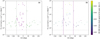 |
Fig. 1. MESSENGER solar energetic electron peak intensities versus CA. The vertical dashed lines indicate the connection angles CA = −65° (left) and CA = +33° (right). The horizontal lines show the truncation level of the sample. (a) Includes all SEE events selected for the study. The colour of the points depends on the CA. The purple square points correspond to the sample of well-connected events, namely −65° ≤ CA ≤ +33°. The rest of the sample is indicated with green circles. (b) Only events accompanied by a CME-driven shock are shown, and these are colour-coded according to the shock speed at the apex. |
5.2. Bayesian probability approach: Kelly method
We also estimated the correlation coefficients between the different variables included in this study using the Bayesian approach by Kelly (2007), hereafter referred to as the Kelly method. Bayesian inference belongs to the category of evidential probabilities: to evaluate the probability of a hypothesis, the prior distribution is specified for each statistical parameter, which quantifies the prior knowledge on the possible values. This, in turn, is subsequently updated to an a posterior probability distribution in the light of new, relevant data (evidence). The Bayesian interpretation provides a standard set of procedures and formulae to perform this calculation. In the Kelly method, a generalised likelihood function for the measured data is constructed and the intrinsic distribution of the independent variables is approximated using a mixture of Gaussian functions instead of using predetermined model distributions. This approach differs from those discussed in the previous section and offers a more robust alternative to the commonly used ordinary least-squares (OLS) methods as it directly accounts for: (1) measurement errors in both the independent and dependent variables in linear regression; (2) intrinsic scatter; and (3) selection effects such as non-detections (e.g. censored or truncated data; Kelly 2007; Feigelson & Babu 2012). The uncertainties in the regression parameters and the correlation coefficient are derived from the posterior distribution of the parameters given the observed data (Kelly 2007). In the following, we present the results using both methods, namely the Spearman and Pearson correlations and the Kelly approach.
5.3. SEE peak intensity versus solar activity parameters
In this section we followed the procedure presented above to estimate the correlations between the SEE peak intensity and the parameters related to their parent solar activity. The different correlation coefficients found in this study are summarised in Table 2 (Spearman and Pearson methods) and Table 3 (Kelly method). Table 2 shows that Spearman and Pearson methods give similar results within the uncertainties. Therefore, in the following sections, when both the Spearman and Pearson coefficients are available, we used the Pearson results to compare with previous studies. The correlation coefficients based on the Kelly method listed in Table 3 are obtained as the median value from the posterior distribution presented above, while the uncertainty of the correlation corresponds to the median absolute deviation (MAD; Feigelson & Babu 2012). As detailed below, we note that the values for the correlation coefficients and uncertainties using the Kelly method are larger than the ones obtained using the Spearman and Pearson methods. This is mainly due to the Kelly method including the measurement errors when estimating the correlation coefficients. The wider credible intervals are a measure of the widths of the posterior distributions and represent larger uncertainties in the estimated parameters (Kelly 2007).
Spearman and Pearson correlations between the variables involved in this study.
5.3.1. SEE peak intensity versus flare location
Figure 1a shows the 71–112 keV electron peak intensities as a function of the CA, which is the longitudinal separation between the flare location and the footpoint of the magnetic field connecting to the spacecraft, as discussed in Sect. 3.2. The events with the largest intensities, between ∼105 and ∼108 (cm2 sr s MeV)−1, are observed on the range −75°≲ CA≲ +38°, including the well-connected events at CA∼0°, with a trend towards negative CA values. We note the asymmetry in the positive and negative CAs. We also estimated the connectivity using a range of solar-wind speeds of 300–500 km s−1, where the CAs varied between −10° and +5°, which does not change the results in the observed asymmetry. Based on this asymmetry, we divided the full sample into well- and poorly connected events using the centroid ϕ0 and sigma σ found by Lario et al. (2013). These authors used a Gaussian to describe the longitudinal distribution of peak intensities for spacecraft near 1 au. In the case of 71–112 keV electrons and using a constant speed of 400 km s−1 for the solar wind speed, Lario et al. (2013) found ϕ0 = −16° ± 3° and σ = 49° ±2°. Therefore, we chose the connection angle interval CA ∈ −16° ± 49°(−65° ≤ CA ≤ +33°) as the well-connected sector. These SEE events are indicated in purple in Fig. 1a. The events shown in green in the figure include the poorly connected events, which tend to have intensities below ∼105 (cm2 sr s MeV)−1. We note that we found a few higher-intensity events (3 out of 29) in the poorly connected sample. The percentage of poorly connected events included in the full sample is of ∼45%. Figure 1b shows that, for the majority (25 out 28) of the poorly connected events, the peak electron intensity ranges from ∼104 to ∼105 (cm2 sr s MeV)−1, independently of the CME-driven shock speed associated to the SEE event. The horizontal lines in Fig. 1 show the truncation level of the sample, related to the elevated background of the particle instrument, which is close to ∼104 (cm2 sr s MeV)−1, as discussed in Sect. 5.1.
5.3.2. SEE peak intensity versus flare intensity
Figure 2a shows the logarithm of the 71–112 keV electron peak intensities plotted against the logarithm of the flare SXR peak flux. The points show the error bars corresponding to the uncertainties of the measurements. The vertical arrows indicate the error in the measured SEE peak intensities due to the anti-Sun pointing of the EPS instrument, as discussed in Sect. 5.1. The colour code of the points is the same as in Fig. 1a. The number of events included in the full sample and well-connected events are given on the top of the panel and in Col. 2 of Table 1. The legend also shows the correlation coefficients for the two different approaches discussed above.
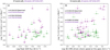 |
Fig. 2. Logarithm of the electron peak intensity against the logarithm of the flare intensity (a) and the logarithm of the maximum speed of the 3D CME-driven shock at the apex (b). The colour code of the points is the same as in Fig. 1a. All the points show the error bars corresponding to the uncertainties of the measurements. The vertical arrows over the points represent the error due to the anti-sunward pointing of the EPS instrument. The legend shows the number of events and the correlation coefficients corresponding to the full list of (well-connected) events in black (purple). Details given in the main text. |
Column 2 of the first row in Table 2 shows that the Spearman correlation between the logarithms of the peak SEE intensity and the flare intensity is weak: cc = 0.32 ± 0.04. This correlation is significantly higher than that (cc = 0.12) found by Dresing et al. (2022) for a subsample of about 40 electron (55–85 keV) events measured near 1 au by STEREO. We note that this latter study also included both well- and poorly connected events. The correlation between the SEE peak intensities and the flare intensity is significantly larger for the well-connected events, with a moderate Pearson correlation coefficient of cc = 0.59 ± 0.03. This value is in agreement with the results of Trottet et al. (2015), who found a correlation of cc = 0.53 ± 0.09 for the 38 electron (175 keV) events in the western solar hemisphere (CA ≃ 0), measured near 1 au by the Advanced Composition Explorer (ACE; Stone et al. 1998).
Similarly, using the Kelly approach (first row, Col. 2, Table 3), the logarithm of the peak intensity shows a weaker correlation with the logarithm of the flare intensity for the full sample (cc = 0.56 ± 0.38) than with that for the well-connected events (cc = 0.74 ± 0.30). In contrast to Spearman and Pearson methods, the Kelly approach gives a moderate (versus weak) and strong (versus moderate) correlation for the two aforementioned samples, respectively.
Correlations between the variables involved in this study based on the Kelly method.
5.3.3. SEE peak intensity versus CME-driven shock speed
Figure 2b shows the logarithm of the 71–112 keV electron peak intensities plotted against the logarithm of the 3D CME-driven shock maximum speed at the apex. The colour code of the points is as in Fig. 1a, and the error bars and legend are similar to those of Fig. 2a. Column 3 of the first row of Table 2 shows that the Spearman correlation between the logarithms of the peak SEE intensity and the 3D CME-driven shock speed at the apex is low: cc = 0.26 ± 0.04. This correlation is similar to that (cc = 0.24) found by Dresing et al. (2022) for the correlation between the logarithm of the peak intensities and the speed (not the logarithm) of the shock apex for a full sample of 33 electron (55–85 keV) events measured near 1 au by the two STEREO spacecraft. We note that Dresing et al. (2022) include both well- and poorly connected events and also used 3D parameters of the coronal shock reconstruction, which resulted in larger correlation coefficients compared to not using 3D parameters.
In the case of well-connected events, indicated in Fig. 1b with the vertical purple lines, the correlation found in this study is significantly larger, with a moderate Pearson correlation coefficient of cc = 0.65 ± 0.04. This correlation is slightly higher than that (cc = 0.49) estimated by Xie (2019), who compared the logarithm of the 62–105 keV electron peak intensities with the 3D shock speed (not the logarithm) for CA = 0 from a sample of events measured during solar cycle 24 by STEREO and ACE.
Similarly, using the Kelly approach (first row, Col. 3, Table 3), the logarithm of the peak intensity shows a weaker correlation with the logarithm of the shock speed for the full sample (cc = 0.68 ± 0.33) than with that for the well-connected events (cc = 0.87 ± 0.20). In contrast to Spearman and Pearson methods, the Kelly approach gives a strong (versus weak) and very strong (versus strong) correlation for the two respective aforementioned samples. We note that the uncertainty for the well-connected events is smaller than for the full sample, and therefore the significance of the correlation is larger.
5.3.4. SEE peak intensity versus CME speed
Figure 3a shows the logarithm of the 71–112 keV electron peak intensities versus the logarithm of the 3D CME speed at the apex. The colour code of the points is as in Fig. 1a. The error bars and legend are similar to those in Fig. 2. Column 4 of the first row in Table 2 shows that the correlation between the logarithms of the peak SEE intensity and the 3D CME speed at the apex is low: cc = 0.23 ± 0.03. This correlation is also significantly larger for the well-connected events, with a moderate Pearson correlation coefficient of cc = 0.46 ± 0.03. This value is slightly lower than that (cc = 0.68 ± 0.09) found by Trottet et al. (2015) for 38 electron (175 keV) events in the western solar hemisphere measured near 1 au by ACE. We note that, in that study, the values of the CME speed were estimated from linear fits to the time–height trajectory of the CME front, as provided in the CME catalogue (Yashiro et al. 2004) of SOHO/LASCO.
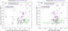 |
Fig. 3. Logarithm of the electron peak intensity against the logarithm of the 3D CME speed at the apex (a) and 3D CME width at the ecliptic plane (b). Colours and legend are as in Fig. 2. |
Similarly, using the Kelly approach (first row, Col. 4, Table 3), the logarithm of the peak intensity shows a weaker correlation with the logarithm of the CME speed for the full sample (cc = 0.47 ± 0.43) than with that for the well-connected events (cc = 0.60 ± 0.39). We note that the correlation for the full sample is not significant, as the uncertainty is similar to the coefficient value. In contrast to Spearman and Pearson methods, the Kelly approach gives a strong (versus moderate) correlation for the well-connected sample. We note that in all the cases, the correlations found here are weaker than that found for the CME-driven shock presented in Sect. 5.3.3.
5.3.5. SEE peak intensity versus CME width
Figure 3b shows the logarithm of the SEE peak intensity versus the logarithm of the 3D CME width in the ecliptic plane. The colour code of the points is as in Fig. 1a. The error bars and legend are similar to those of Fig. 2a. Column 5 of the first row in Table 2 shows that the correlation between the logarithms of the peak SEE intensity and the 3D CME width is low: cc = 0.21 ± 0.04. This value is in agreement with Kahler et al. (1999), who found a similar weak correlation (cc = 0.28) between the angular width of the CME and the logarithm of the proton peak intensities. The correlation is not significantly stronger for well-connected events, with a low Pearson correlation coefficient of cc = 0.26 ± 0.04.
Using the Kelly approach (first row, Col. 5, Table 3), the logarithm of the peak intensity shows a stronger correlation with the logarithm of the CME width for the full sample (cc = 0.52 ± 0.36) than with that for the well-connected events (cc = 0.27 ± 0.44). We note that the uncertainty is higher than the correlation coefficient in the case of the well-connected sample, and so the correlation is not significant.
5.4. SEE peak-intensity energy spectra versus coronal shock speed and flare intensity
In Paper I, the peak-intensity energy spectra of 42 SEE events measured by the MESSENGER mission were analysed. The energies used in the analysis ranged from ∼71 keV to ∼1 MeV divided into six energy bins. For each of the events, the authors took the time-of-maximum intensity based on the 71–112 keV channel using one-hour averages and read the intensity peak at this time for the rest of the energy channels. For all the events, the fitting resembled a single power law, giving the spectral index and its uncertainty, namely δ200, as shown in Col. 11 of Table A.1. Figures 4a,b show the spectral indices against the logarithm of the maximum speed of the 3D CME-driven shock at the apex and the logarithm of the flare intensity, respectively. The colour code of the points is the same as in Fig. 1a. We find no correlation between any of these measurements. This result is in agreement with Dresing et al. (2022), who found no clear correlations between the shock parameters and the spectral indices of the near-relativistic electrons. We do not observe harder spectra with increasing peak intensities (not shown) as Kahler (2001) found for high energy protons (> 10 MeV).
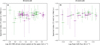 |
Fig. 4. MESSENGER solar energetic electron spectral indices against the CME-driven shock speed at the apex (a) and the SXR intensity of the flare (b). The colour code of the points is as in Fig. 1a. |
5.5. Relations between the solar parent activity
The last three rows of Tables 2 and 3 show the correlations between the variables describing the solar activity. There is a moderate correlation between the logarithms of the flare intensity and the 3D CME-driven shock speed (Pearson: cc = 0.53 ± 0.04; Kelly: cc = 0.60 ± 0.12; 33 events) and the 3D CME speed (Pearson: cc = 0.57 ± 0.03, Kelly: cc = 0.61 ± 0.11; 36 events). This last value is similar to the correlation coefficient (Pearson: cc = 0.66) obtained by Kihara et al. (2020) when sampling 79 events from 2006 to 2014 with near 1 au spacecraft. We note that Kihara et al. (2020) use the CME speed instead of the logarithm of this variable. The correlation between the maximum speed of the 3D CME-driven shock and the speed of the 3D CME is strong (Pearson: cc = 0.81 ± 0.02; Kelly: cc = 0.88 ± 0.04; 52 events). There is a weak correlation between the width of the 3D CME and all of the other variables.
6. Summary and discussion
We used the list of 61 SEE events measured by the MESSENGER mission from 2010 to 2015 presented in Paper I, which is when the heliocentric distance of the spacecraft varied from 0.31 au to 0.47 au. Due to the elevated background intensity level of the particle instrument on board MESSENGER, the SEE events measured by this mission are necessarily large and intense; most of them are accompanied by a CME-driven shock, are widespread in heliolongitude, and display relativistic (∼1 MeV) electron intensity enhancements. The largest peak intensities, between ∼105 and ∼108 (cm2 sr s MeV)−1, are observed in the range of connection angles −75° < CA < +38°, with an asymmetry to longitudes east of the well-connected longitudes CA ∼ 0°.
To relate the near-relativistic electron peak intensity and the peak-intensity energy spectra to different parameters of the parent solar source, we (1) considered the flare peak intensity measured in Paper I from the events originating on the visible side of the Sun from Earth’s point of view and (2) took advantage of the multi-viewpoint spacecraft observations to reconstruct, when possible, the large-scale 3D structure of the CME and the CME-driven shock using the GCS model (Thernisien 2011) and the ellipsoid model (Kwon et al. 2014), respectively. We added some of the reconstructed parameters to the list of SEE events in Table A.1 for future reference.
6.1. Summary of observational results
In this work, we first characterised the distribution of the samples in order to select the appropriate method to estimate the correlation coefficients between the SEE peak intensity and energy spectra and several parameters related to the solar activity. We also addressed the fact that the peak intensities measured by MESSENGER were truncated and presented asymmetric uncertainties due to instrumental limitations (elevated background level, anti-sunward pointing). The observational results of this study can be summarised as follows:
-
There is an asymmetry in the positive and negative connection angles for which the largest intensities are measured. This asymmetry is therefore considered in the definition of the connection angle interval in the so-called well-connected events, namely −65° ≤ CA ≤ +33°, in which we find stronger correlations between the SEE peak intensities and the solar parameters in comparison to the full sample.
-
In the majority of the poorly connected events, the peak intensities are below ∼105 (cm2 sr s MeV)−1, independently of the intensity of the flare or the speed of the CME-driven shock. A poor connectivity to the source weakens the correlations between the peak intensities and the different parent solar source parameters.
-
The strongest correlations are found between the near-relativistic electron peak intensities and the maximum speed at the apex of the 3D CME-driven shock and the flare intensity for the so-called well-connected events. The Pearson correlation coefficients and their uncertainties based on a Monte Carlo method are: cc = 0.65 ± 0.04 (shock) and cc = 0.59 ± 0.03 (flare). We note the similar correlations between the SEE peak intensities and the maximum speed of the 3D CME-driven shock at the apex and the flare intensity. The correlation coefficients based on the Kelly method are cc = 0.87 ± 0.20 (shock) and cc = 0.74 ± 0.30 (flare). We also note the reduced uncertainty in the case of the shock sample compared to the correlations with other solar parameters.
-
We find a moderate correlation between the near-relativistic electron peak intensities and the CME speed at the apex for the well-connected events, with a Pearson (Kelly) correlation coefficient of cc = 0.46 ± 0.03 (cc = 0.60 ± 0.39).
-
The weakest correlations for the well-connected events are found between the near-relativistic electron peak intensities and the 3D CME width, with a Pearson (Kelly) correlation coefficient of cc = 0.26 ± 0.04 (cc = 0.27 ± 0.44). We note that in the Kelly method, the uncertainty is higher than the correlation coefficient, indicating that no significant correlation can be determined.
-
The correlations between the near-relativistic electron peak intensities and the solar activity – namely the flare intensity and the speed of the 3D CME-driven shock – estimated in this study are higher than those found by two equivalent studies based on near 1 au measurements, namely, Dresing et al. (2022) and Xie (2019). However, we note that in the study by Trottet et al. (2015), the correlations with the flare intensity are similar.
-
We find no correlation between the spectral indices and either the flare intensity or the CME-driven shock speed.
-
Correlations of similar order exist between the different parameters describing solar activity, such as flare intensity, CME speed, and CME-driven shock. The correlation between the solar-activity parameters (e.g. flare intensity and shock speed) is smaller than the correlations between the SEE peak intensities and either the flare intensity or the shock speed.
6.2. Effect on the interpretation of the origin of SEEs
6.2.1. Correlations between the parameters characterising the solar activity
One of the difficulties found when interpreting statistical relations between solar activity and SEEs is the interrelationship of the different parameters utilised to characterise the solar activity, as summarised in the last three rows of Tables 2 and 3. For example, Kahler (1982) introduced the term ‘big flare syndrome’ to illustrate the observational fact that there is a correlation between any two parameters measuring the magnitude of a flare event, independent of the detailed physical relationship between them. In this study, we find a moderate correlation between the SXR peak flux and the CME speed (Pearson: cc = 0.57 ± 0.03; Kelly: cc = 0.61 ± 0.11). This correlation might be related to a common physical process at the Sun. It is well known that the acceleration of CMEs is closely related in time with the evolution of thermal energy release in the associated flare (Zhang et al. 2004; Bein et al. 2012), suggesting an interdependence between the CME speed and the peak flux of the flare.
As expected, we find a strong correlation between the maximum speed of the 3D CME-driven shock at the apex and the speed of the 3D CME at the apex derived from a linear fit of the time evolution of the CME apex height (Pearson: cc = 0.81 ± 0.02; Kelly: cc = 0.88 ± 0.04). This correlation might be expected to be even higher (i.e. closer to cc = 1). A reason for the relatively low value we find could be related to measuring the maximum speed for the shock but the average linear speed for the CME. Lastly, we find a moderate correlation between the flare intensity and the speed of the 3D CME-driven shock (Pearson: cc = 0.53 ± 0.04; Kelly: cc = 0.60 ± 0.12), which might be related to both the intrinsic relation between the flare intensity and the CME speed, and the relation between the CME speed and the CME-driven shock speed, as discussed above.
Using partial correlations in the analysis of the relations between SEE parameters and the solar activity (e.g. Trottet et al. 2015) might be a simplification of the real picture, as the correlations between variables actually show a degeneracy in the parameter space. The flare-related and CME-related phenomena are expressions of the solar activity and it is very probable that both share the same common origin at the Sun. Furthermore, based on previous studies, it is probable that using different parameters to characterise the solar activity, such as the fluence for the flare activity (Trottet et al. 2015) or the CME-driven shock speed at the cobpoint (Heras et al. 1995) for the shock activity (Dresing et al. 2022), would increase the correlations with the peak intensities.
6.2.2. Correlation between SEE intensities and solar activity
Our study finds a distinct difference between the SEE correlations found for different samples when classifying them by connection angle. For the full sample of the events, including poorly connected events, we find similar weak Pearson correlations between the SEE peak intensities and the different quantities that describe the solar activity, varying from cc ∼0.21 to ∼0.32. Also, the uncertainty found in the correlations based on the Kelly method are significant with respect to the correlation coefficient, meaning that the correlations are not clear. This is expected because of the inclusion of the poorly connected events in the study, where the transport effects and/or the connection to peripheral areas of the source (shock) could significantly distort the correlations. This behaviour is clearly observed in Fig. 1b, where the majority of the points outside the purple vertical lines – which indicate the well-connected range – are showing intensities of between ∼104 and ∼105 (cm2 sr s MeV)−1 independently of the shock speed. The few high-intensity points outside the well-connected range might be related to varying CME widths and/or different footpoint locations caused by non-nominal solar-wind speed or disturbed Parker-field.
However, for the well-connected events, namely for −65° ≤ CA ≤ 33°, we generally find clearer correlations. The SEE peak intensities correlate similarly with the 3D CME-driven maximum shock speed (Pearson: cc = 0.65 ± 0.04; Kelly: cc = 0.87 ± 0.20) and with the SXR peak flux (Pearson: cc = 0.59 ± 0.03; Kelly: cc = 0.74 ± 0.30). We note the lower uncertainties found in the Kelly method between the SEE peak intensities and the shock speed in comparison with the flare intensity. However, the samples are not the same, as we are not considering far-side events for the flare intensity and this fact could affect the comparison between correlations. These correlations are stronger than those found for CME speed (Pearson: cc = 0.46 ± 0.03; Kelly: cc = 0.60 ± 0.39). Therefore, the correlation of the peak electron intensity with the maximum speed of the 3D CME-driven shock at the apex is stronger and also more significant than that with the CME speed at the apex. This means that the maximum shock speed might be a better proxy for the acceleration of energetic electrons than the linear CME speed.
For the well-connected events, we also find that the correlation between the logarithms of the peak intensity of the SEE events and the speed of the CME-driven shock at the apex is stronger in the SEE events measured by MESSENGER (Pearson: cc = 0.65 ± 0.04; Kelly: cc = 0.87 ± 0.20) in comparison to near 1 au data (Pearson: cc = 0.49) for similar near-relativistic energies and using CME and associated 3D shock parameters (Xie 2019). We note that Xie (2019) uses the speed of the shock instead of the logarithm of the shock speed. However, the results are similar when directly comparing the shock speed in both studies. Similarly, the correlation between the peak intensities and the flare intensity for the full sample (Pearson: cc = 0.32 ± 0.04; Kelly: cc = 0.56 ± 0.38) is higher than that found for near 1 au measurements (Pearson: cc = 0.12; Dresing et al. 2022), which include both well- and poorly connected events. In the case of well-connected events (−65° ≤ CA ≤ 33°), we find similar correlations (Pearson: cc = 0.59 ± 0.03; Kelly: cc = 0.74 ± 0.30) to Trottet et al. (2015), who use near 1 au data (Pearson: cc = 0.53 ± 0.09).
On a statistical basis, the CME width seems not to play a relevant role in terms of the peak intensity of the SEE event, as the correlations for both the full sample and well-connected events are weak. We note that we find slightly stronger correlations between the peak intensities and the CME width estimated as in Dumbović et al. (2019), which takes the tilt of the CME into account (Pearson: cc = 0.21 ± 0.04 for the full sample, cc = 0.26 ± 0.04 for the well-connected events), than between the peak intensities and the face-on width of the CME (Pearson: cc = 0.11 ± 0.05, cc = 0.16 ± 0.05, not shown). In the case of the spectral indices, in addition to the large uncertainties, we suspect that the missing correlations might be partly due to a selection effect, as MESSENGER is mostly measuring large events, the majority of them being widely spread in the heliosphere and with the presence of relativistic electron enhancements. The spectral indices in the MESSENGER sample are mainly hard, with a mean of δ200 = −1.9 ± 0.3, as can be observed in Fig. 4, while SEE spectra in general can be much softer (e.g. Dresing et al. 2020).
6.2.3. Other quantities affecting the peak intensities
The conditions of particle acceleration and propagation in the high corona and interplanetary space affect SEP intensities. The pre-event intensity level might also play a role. Figure 2b shows that, for the well-connected events (purple points), the peak SEE intensities associated with a CME-driven shock of a given speed vary over about four orders of magnitude, similar to the result found by Kahler (2001), who used pre-event background-subtracted SEE peak intensities. This could be interpreted as evidence for a supra-thermal seed population that made local shock acceleration more efficient. Other factors related to observing a range of peak intensities for a given speed might be the dynamic connection between MESSENGER and the travelling shock, and the presence of previous disturbances in the IP space that may affect the interplanetary magnetic-field structure in which SEEs propagate.
The asymmetry in the positive and negative angles delimiting the subsample of events with the highest peak intensities might be associated with several processes. A possible scenario could be related to acceleration mechanisms in the shock environment at a certain height from the Sun and the evolution of magnetic field connection to the shock front (e.g. Lario et al. 2014; Ding et al. 2022), where the maximum peak intensity is observed when the flare occurs eastward of the magnetic footpoint of the spacecraft. For example, the nominal best connection for an observer near 0.4 au, using a speed of 400 km s−1, to a source at W30 is modified by a CME-driven shock that moves out radially so that the connection to its apex is further towards the east than W30. Perpendicular diffusion processes during the transport of SEPs in the heliosphere might also be related to this asymmetry (e.g. He & Wan 2015).
As MESSENGER lacks solar-wind measurements, the magnetic separation angle, which is determined with an assumed solar-wind speed of 400 km s−1, could deviate significantly. However, as discussed above, we obtained similar results regarding the observed asymmetry when using a range of solar-wind speeds of 300–500 km s−1. We also clearly observe in this study that the poor connectivity to the solar source blurs the correlation between the peak intensities and the solar activity. This might be related to the poorly connected events being affected by transport effects and/or to the connection to weaker parts of a shock, as discussed in Sect. 6.2.2.
6.3. Final discussion
The strongest correlations found in this study between the near-relativistic electron peak intensities and the solar activity are with the speed of the 3D CME-driven shock and the flare intensity. This is statistical confirmation of the idea that both flare and shock-related processes may contribute to the acceleration of near-relativistic electrons in large SEE events (Kallenrode 2003; Trottet et al. 2015; Dresing et al. 2022) provided the flare-accelerated particles escape to interplanetary space. The correlations found between the flare intensity and the shock speed being lower than the correlations between the SEE peak intensities and the flare intensity or the shock speed might support this result.
Also, we find a stronger correlation between the SEE peak intensities and the maximum speed of the 3D CME-driven shock than with the 3D CME speed. This means that the maximum speed of the CME-driven shock, usually observed below 10 R⊙, is a better proxy with which to investigate particle-acceleration-related mechanisms than the CME speed from linear fits to the height–time profile in the coronagraph field of view, as usually used in the past (e.g. Trottet et al. 2015; Kihara et al. 2020).
Closer to the Sun (i.e. closer to the acceleration site), we find stronger correlations with the solar parameters associated with the electron-acceleration mechanisms when compared to some of the previous studies using near 1 au data. This difference is more relevant when comparing studies with similar connectivity and using the 3D parameters of the CME-related activity (Xie 2019; Dresing et al. 2022). This suggests that the effect of the IP transport from near 0.3 au to near 1 au on the energetic electrons might weaken the correlations between the solar source parameters and the peak intensities measured in situ. However, the correlations found by Trottet et al. (2015) are similar as those found in this study. Future studies with the same samples and following the same methodology near 0.3 au and near 1 au are therefore necessary to investigate this possible effect of the IP transport further.
Two interesting observational results of this study are (1) the asymmetry to the east of the range of connection angles for which the SEE events present the highest peak intensities, and (2) the presence of relativistic electrons in 37 out of 61 SEE events. Previous studies related these observations to different acceleration mechanisms. In the case of the presence of MeV electrons, both flare-related (e.g. Simnett 1974) and shock-related (e.g. Kahler 2007; Dresing et al. 2022) scenarios have been suggested. In the case of the asymmetry to the east, it has been attributed to diverse factors, such as acceleration mechanisms in the shock environment (e.g. Lario et al. 2014; Ding et al. 2022) or the role of perpendicular diffusion in the particle transport (e.g. He & Wan 2015), as discussed above. Based on the comparison of the correlation coefficients presented in this study alone, we do not find any statistical indication that favours one mechanism over another (i.e. the differences in the correlation coefficients are not statistically significant). Therefore, the analysis and outcomes presented here might be further investigated with data from the new ongoing missions exploring the innermost regions of the heliosphere, such as Solar Orbiter (Müller 2020; Zouganelis et al. 2020), Parker Solar Probe (PSP; Fox et al. 2016) and BepiColombo (Benkhoff et al. 2010), together with near 1 au missions remotely observing the Sun. Alternative parameters related to the solar activity, such as the SXR fluence, the CME expansion speed in the early phases close to the Sun surface, and shock characteristics at the cobpoint, which might better describe the strength of the probable accelerators (Trottet et al. 2015; Dresing et al. 2022), could also be investigated in future studies. Using these new multi-spacecraft observations, and as we progress into solar cycle 25, we will measure more events and increase the statistics, which will allow a reduction of the uncertainties.
Acknowledgments
The UAH team acknowledges the financial support by the Spanish Ministerio de Ciencia, Innovación y Universidades FEDER/MCIU/AEI Projects ESP2017-88436-R and PID2019-104863RB-I00/AEI/10.13039/501100011033 and by the European Union’s Horizon 2020 research and innovation program under grant agreement No. 101004159 (SERPENTINE). LRG is also supported by the European Space Agency, under the ESA/NPI program and thanks Karl Ludwig Klein, Angelos Vourlidas, and Nariaki Nitta for their help. LAB acknowledges the support from the NASA program NNH17ZDA001N-LWS (Awards Nr. 80NSSC19K0069 and 80NSSC19K1235). AK acknowledges financial support from NASA NNN06AA01C (SO-SIS Phase-E) contract. ND is grateful for support by the Turku Collegium for Science, Medicine and Technology of the University of Turku, Finland and acknowledges the support of Academy of Finland (SHOCKSEE, grant 346902). DL acknowledges support from NASA Living With a Star (LWS) programs NNH17ZDA001N-LWS and NNH19ZDA001N-LWS, and the Goddard Space Flight Center Internal Scientist Funding Model (competitive work package) program and the Heliophysics Innovation Fund (HIF) program. The authors acknowledge the different SOHO, STEREO instrument teams, and the STEREO and ACE science centers for providing the data used in this paper. This research has used PyThea v0.7.3, an open-source and free Python package to reconstruct the 3D structure of CMEs and shock waves (GCS and ellipsoid model).
References
- Agueda, N., & Lario, D. 2016, ApJ, 829, 131 [NASA ADS] [CrossRef] [Google Scholar]
- Andrews, G. B., Zurbuchen, T. H., Mauk, B. H., et al. 2007, Space Sci. Rev., 131, 523 [CrossRef] [Google Scholar]
- Bein, B. M., Berkebile-Stoiser, S., Veronig, A. M., Temmer, M., & Vršnak, B. 2012, ApJ, 755, 44 [NASA ADS] [CrossRef] [Google Scholar]
- Benkhoff, J., van Casteren, J., Hayakawa, H., et al. 2010, Planet Space Sci., 58, 2 [CrossRef] [Google Scholar]
- Brueckner, G. E., Howard, R. A., Koomen, M. J., et al. 1995, Sol. Phys., 162, 357 [NASA ADS] [CrossRef] [Google Scholar]
- Curran, P. A. 2015, Astrophysics Source Code Library [record ascl:1504.008] [Google Scholar]
- D’Agostino, R., & Pearson, E. S. 1973, Biometrika, 60, 613 [Google Scholar]
- Ding, Z., Li, G., Ebert, R. W., et al. 2022, J. Geophys. Res. Space Phys., 127, e2022JA030343 [CrossRef] [Google Scholar]
- Domingo, V., Fleck, B., & Poland, A. I. 1995, Sol. Phys., 162, 1 [Google Scholar]
- Dresing, N., Gómez-Herrero, R., Heber, B., et al. 2014, ApJ, 567, A27 [Google Scholar]
- Dresing, N., Theesen, S., Klassen, A., & Heber, B. 2016, A&A, 588, A17 [NASA ADS] [CrossRef] [EDP Sciences] [Google Scholar]
- Dresing, N., Effenberger, F., Gómez-Herrero, R., et al. 2020, ApJ, 889, 143 [NASA ADS] [CrossRef] [Google Scholar]
- Dresing, N., Kouloumvakos, A., Vainio, R., & Rouillard, A. 2022, ApJ, 925, L21 [NASA ADS] [CrossRef] [Google Scholar]
- Dumbović, M., Guo, J., Temmer, M., et al. 2019, ApJ, 880, 18 [Google Scholar]
- Feigelson, E. D., & Babu, G. J. 2012, Modern Statistical Methods for Astronomy (Cambridge University Press) [Google Scholar]
- Fox, N. J., Velli, M. C., Bale, S. D., et al. 2016, Space Sci. Rev., 204, 7 [Google Scholar]
- García, H. A. 1994, Sol. Phys., 154, 275 [NASA ADS] [CrossRef] [Google Scholar]
- Gieseler, J., Dresing, N., Palmroos, C., et al. 2023, Front. Astron. Space Phys., 9, 384 [NASA ADS] [Google Scholar]
- He, H. Q., & Wan, W. 2015, ApJS, 218, 17 [NASA ADS] [CrossRef] [Google Scholar]
- Heras, A. M., Sanahuja, B., Lario, D., et al. 1995, ApJ, 445, 497 [NASA ADS] [CrossRef] [Google Scholar]
- Howard, R. A., Moses, J. D., Vourlidas, A., et al. 2008, Space Sci. Rev., 136, 67 [NASA ADS] [CrossRef] [Google Scholar]
- Kahler, S. W. 1982, J. Geophys. Res., 87, 3439 [NASA ADS] [CrossRef] [Google Scholar]
- Kahler, S. W. 2001, J. Geophys. Res., 106, 20947 [NASA ADS] [CrossRef] [Google Scholar]
- Kahler, S. W. 2007, Space Sci. Rev., 129, 359 [NASA ADS] [CrossRef] [Google Scholar]
- Kahler, S. W., & Hundhausen, A. J. 1992, J. Geophys. Res., 97, 1619 [NASA ADS] [CrossRef] [Google Scholar]
- Kahler, S., Burkepile, J., & Reames, D. 1999, Int. Cosmic R. Conf., 6, 248 [NASA ADS] [Google Scholar]
- Kaiser, M. L., Kucera, T. A., Davila, J. M., et al. 2008, Space Sci. Rev., 136, 5 [Google Scholar]
- Kallenrode, M. B. 2003, J. Phys. G Nucl. Phys., 29, 965 [Google Scholar]
- Kelly, B. C. 2007, ApJ, 665, 1489 [Google Scholar]
- Kihara, K., Huang, Y., Nishimura, N., et al. 2020, ApJ, 900, 75 [NASA ADS] [CrossRef] [Google Scholar]
- Klein, K. L., Krucker, S., Trottet, G., & Hoang, S. 2005, A&A, 431, 1047 [NASA ADS] [CrossRef] [EDP Sciences] [Google Scholar]
- Kokoska, S., & Zwillinger, D. 2000, CRC Standard Probability and Statistics Tables and Formulae (New York, NY: Springer), 502 [Google Scholar]
- Kouloumvakos, A., Nindos, A., Valtonen, E., et al. 2015, A&A, 580, A80 [NASA ADS] [CrossRef] [EDP Sciences] [Google Scholar]
- Kouloumvakos, A., Patsourakos, S., Nindos, A., et al. 2016, ApJ, 821, 31 [NASA ADS] [CrossRef] [Google Scholar]
- Kouloumvakos, A., Rouillard, A. P., Wu, Y., et al. 2019, ApJ, 876, 80 [NASA ADS] [CrossRef] [Google Scholar]
- Kouloumvakos, A., Rodríguez-García, L., Gieseler, J., et al. 2022, Front. Astron. Space Sci., 9, 15 [CrossRef] [Google Scholar]
- Kowalski, P. 1972, J. R. Stat. Soc. Ser. C (Appl. Stat.), 21, 1 [Google Scholar]
- Krucker, S., Kontar, E. P., Christe, S., Glesener, L., & Lin, R. P. 2011, ApJ, 742, 82 [Google Scholar]
- Kunow, H., Wibberenz, G., Green, G., Müller-Mellin, R., & Kallenrode, M.-B. 1991, in Physics of the Inner Heliosphere II (Springer-Verlag), 243 [NASA ADS] [CrossRef] [Google Scholar]
- Kwon, R.-Y., Zhang, J., & Olmedo, O. 2014, ApJ, 794, 148 [NASA ADS] [CrossRef] [Google Scholar]
- Lario, D., Ho, G. C., Decker, R. B., et al. 2003, Am. Inst. Phys. Conf. Ser., 679, 640 [Google Scholar]
- Lario, D., Aran, A., Gómez-Herrero, R., et al. 2013, ApJ, 767, 41 [CrossRef] [Google Scholar]
- Lario, D., Roelof, E. C., & Decker, R. B. 2014, ASP Conf. Ser., 484, 98 [NASA ADS] [Google Scholar]
- Lemen, J. R., Title, A. M., Akin, D. J., et al. 2012, Sol. Phys., 275, 17 [Google Scholar]
- Maia, D. J. F., & Pick, M. 2004, ApJ, 609, 1082 [NASA ADS] [CrossRef] [Google Scholar]
- Müller, D., St Cyr, O. C., Zouganelis, I., et al. 2020, A&A, 642, A1 [Google Scholar]
- Nitta, N. V., Aschwanden, M. J., Boerner, P. F., et al. 2013, Sol. Phys., 288, 241 [Google Scholar]
- Papaioannou, A., Sandberg, I., Anastasiadis, A., et al. 2016, J. Space Weather Space Clim., 6, A42 [NASA ADS] [CrossRef] [EDP Sciences] [Google Scholar]
- Pesnell, W. D., Thompson, B. J., & Chamberlin, P. C. 2012, Sol. Phys., 275, 3 [Google Scholar]
- Richardson, I. G., von Rosenvinge, T. T., Cane, H. V., et al. 2014, Sol. Phys., 289, 3059 [NASA ADS] [CrossRef] [Google Scholar]
- Rodríguez-García, L., Gómez-Herrero, R., Zouganelis, I., et al. 2021, A&A, 653, A137 [NASA ADS] [CrossRef] [EDP Sciences] [Google Scholar]
- Rodríguez-García, L., Nieves-Chinchilla, T., Gómez-Herrero, R., et al. 2022, A&A, 662, A45 [NASA ADS] [CrossRef] [EDP Sciences] [Google Scholar]
- Rodríguez-García, L., Gómez-Herrero, R., Dresing, N., et al. 2023, A&A, 670, A51 [NASA ADS] [CrossRef] [EDP Sciences] [Google Scholar]
- Simnett, G. M. 1974, Space Sci. Rev., 16, 257 [CrossRef] [Google Scholar]
- Simnett, G. M., Roelof, E. C., & Haggerty, D. K. 2002, ApJ, 579, 854 [NASA ADS] [CrossRef] [Google Scholar]
- Solomon, S. C., McNutt, R. L., Gold, R. E., & Domingue, D. L. 2007, Space Sci. Rev., 131, 3 [NASA ADS] [CrossRef] [Google Scholar]
- Spearman, C. 1987, Am. J. Psychol., 100, 441 [CrossRef] [Google Scholar]
- Stephens, M. A. 1974, J. Am. Stat. Assoc., 69, 730 [CrossRef] [Google Scholar]
- Stone, E. C., Frandsen, A. M., Mewaldt, R. A., et al. 1998, Space Sci. Rev., 86, 1 [Google Scholar]
- Thernisien, A. 2011, ApJS, 194, 33 [Google Scholar]
- Thernisien, A. F. R., Howard, R. A., & Vourlidas, A. 2006, ApJ, 652, 763 [Google Scholar]
- Thernisien, A., Vourlidas, A., & Howard, R. A. 2009, Sol. Phys., 256, 111 [Google Scholar]
- Trottet, G., Samwel, S., Klein, K. L., Dudok de Wit, T., & Miteva, R. 2015, Sol. Phys., 290, 819 [Google Scholar]
- Wall, J. V., & Jenkins, C. R. 2003, Practical Statistics for Astronomers, Vol. 3 (Cambridge University Press) [CrossRef] [Google Scholar]
- West, S. G., Finch, J. F., Curran, P. J., & Hoyle, R. 1995, in Structural Equation Modeling: Concepts, Issues, and Applications, ed. R. H. Hoyle (Sage), 56 [Google Scholar]
- Wuelser, J. P., Lemen, J. R., Tarbell, T. D., et al. 2004, SPIE Conf. Ser., 5171, 111 [NASA ADS] [Google Scholar]
- Xie, H., St. Cyr, O. C., Mäkelä, P., & Gopalswamy, N. 2019, J. Geophys. Res. (Space Phys.), 124, 6384 [NASA ADS] [CrossRef] [Google Scholar]
- Yashiro, S., Gopalswamy, N., Michalek, G., et al. 2004, J. Geophys. Res. (Space Phys.), 109, A07105 [NASA ADS] [CrossRef] [Google Scholar]
- Zhang, J., Dere, K. P., Howard, R. A., & Vourlidas, A. 2004, ApJ, 604, 420 [NASA ADS] [CrossRef] [Google Scholar]
- Zouganelis, I., De Groof, A., Walsh, A. P., et al. 2020, A&A, 642, A3 [NASA ADS] [CrossRef] [EDP Sciences] [Google Scholar]
Appendix A: Solar energetic electron events measured by the MESSENGER mission
Solar energetic electron events measured by MESSENGER.
All Tables
Summary of the statistical properties of the different samples analysed in this study.
Correlations between the variables involved in this study based on the Kelly method.
All Figures
|
Fig. 1. MESSENGER solar energetic electron peak intensities versus CA. The vertical dashed lines indicate the connection angles CA = −65° (left) and CA = +33° (right). The horizontal lines show the truncation level of the sample. (a) Includes all SEE events selected for the study. The colour of the points depends on the CA. The purple square points correspond to the sample of well-connected events, namely −65° ≤ CA ≤ +33°. The rest of the sample is indicated with green circles. (b) Only events accompanied by a CME-driven shock are shown, and these are colour-coded according to the shock speed at the apex. |
| In the text | |
|
Fig. 2. Logarithm of the electron peak intensity against the logarithm of the flare intensity (a) and the logarithm of the maximum speed of the 3D CME-driven shock at the apex (b). The colour code of the points is the same as in Fig. 1a. All the points show the error bars corresponding to the uncertainties of the measurements. The vertical arrows over the points represent the error due to the anti-sunward pointing of the EPS instrument. The legend shows the number of events and the correlation coefficients corresponding to the full list of (well-connected) events in black (purple). Details given in the main text. |
| In the text | |
|
Fig. 3. Logarithm of the electron peak intensity against the logarithm of the 3D CME speed at the apex (a) and 3D CME width at the ecliptic plane (b). Colours and legend are as in Fig. 2. |
| In the text | |
|
Fig. 4. MESSENGER solar energetic electron spectral indices against the CME-driven shock speed at the apex (a) and the SXR intensity of the flare (b). The colour code of the points is as in Fig. 1a. |
| In the text | |
Current usage metrics show cumulative count of Article Views (full-text article views including HTML views, PDF and ePub downloads, according to the available data) and Abstracts Views on Vision4Press platform.
Data correspond to usage on the plateform after 2015. The current usage metrics is available 48-96 hours after online publication and is updated daily on week days.
Initial download of the metrics may take a while.