| Issue |
A&A
Volume 696, April 2025
|
|
|---|---|---|
| Article Number | A12 | |
| Number of page(s) | 9 | |
| Section | The Sun and the Heliosphere | |
| DOI | https://doi.org/10.1051/0004-6361/202453000 | |
| Published online | 28 March 2025 | |
Detection asymmetry in solar energetic particle events
1
Jeremiah Horrocks Institute, University of Central Lancashire, Preston PR1 2HE, UK
2
Heliophysics Division, NASA Goddard Space Flight Center, Greenbelt, MD 20771, USA
3
Department of Physics, University of Maryland, Baltimore County, 1000 Hilltop Circle, Baltimore, MD 21250, USA
4
Secure System Platform Research Laboratories, NEC Corporation, Kanagawa 211-8666, Japan
5
Astronomical Observatory, Kyoto University, Sakyo, Kyoto 606-8502, Japan
6
Lockheed Martin Advanced Technology Center, 3251 Hanover Street, Palo Alto, CA 94304, USA
7
European Space Agency (ESA), European Space Astronomy Centre (ESAC), Camino Bajo del Castillo s/n, 28692 Villanueva de la Cañada, Madrid, Spain
8
Universidad de Alcalá, Space Research Group (SRG-UAH), Plaza de San Diego s/n, 28801 Alcalá de Henares, Madrid, Spain
9
University Corporation for Atmospheric Research, 3090 Center Green Dr., Boulder, CO 80301, USA
⋆ Corresponding author; sdalla@uclan.ac.uk
Received:
14
November
2024
Accepted:
15
February
2025
Context. Solar energetic particles (SEPs) are detected in interplanetary space in association with solar flares and coronal mass ejections (CMEs). The magnetic connection between the observing spacecraft and the solar active region (AR) source of the event is a key parameter in determining whether SEPs are observed and the particle event’s properties.
Aims. We investigate whether an east-west asymmetry in the detection of SEP events is present in observations and discuss its possible link to the corotation of magnetic flux tubes with the Sun.
Methods. We used a published dataset of 239 CMEs recorded between 2006 and 2017 that had source regions both on the Sun’s front and far sides as seen from Earth. We produced distributions of occurrences of in situ SEP intensity enhancements associated with the CME events versus Δϕ, the longitudinal separation between the source AR and the spacecraft magnetic footpoint based on the nominal Parker spiral. We focussed on protons of energy > 10 MeV measured by STEREO A, STEREO B, and GOES at 1 au. We also considered occurrences of 71–112 keV electron events detected by MESSENGER between 0.31 and 0.47 au.
Results. We find an east-west asymmetry with respect to the best magnetic connection (Δϕ = 0) in the detection of > 10 MeV proton events and of 71–112 keV electron events. For protons, observers for which the source AR is on the eastern side of the spacecraft footpoint and not well connected (−180° < Δϕ < −40°) are 93% more likely to detect an SEP event compared to observers with +40° < Δϕ < +180°. The asymmetry may be a signature of the corotation of magnetic flux tubes with the Sun since, for events with Δϕ < 0, corotation sweeps particle-filled flux tubes towards the observing spacecraft, while for Δϕ > 0 it moves them away. Alternatively, it may be related to asymmetric acceleration or propagation effects.
Key words: Sun: activity / Sun: coronal mass ejections (CMEs) / Sun: flares / Sun: heliosphere / Sun: particle emission
© The Authors 2025
 Open Access article, published by EDP Sciences, under the terms of the Creative Commons Attribution License (https://creativecommons.org/licenses/by/4.0), which permits unrestricted use, distribution, and reproduction in any medium, provided the original work is properly cited.
This article is published in open access under the Subscribe to Open model. Subscribe to A&A to support open access publication.
1. Introduction
Solar energetic particles (SEPs), accelerated as a result of energy release events at the Sun, are detected by spacecraft instruments in interplanetary space in close temporal coincidence with flares and coronal mass ejections (CMEs). Time-intensity profiles of electrons, protons, and heavy ions have been characterised extensively over several decades of particle observations (e.g. Van Hollebeke et al. 1975; Cane et al. 1988; Richardson et al. 2014; Papaioannou et al. 2016; Cohen et al. 2017; Rodríguez-García et al. 2023b). During so-called gradual SEP events, intensities measured at 1 au often remain elevated above the background for several days (e.g. Desai & Giacalone 2016; Klein & Dalla 2017; Cohen et al. 2021).
A striking feature of SEP observations is the so-called east-west (E–W) effect in the particle intensity profiles: for a near-Earth spacecraft, events with a source active region (AR) in the west of the Sun tend to have a fast rise to peak intensity and decay, while those with a source AR in the east typically have a slow rise and a longer duration (Cane et al. 1988). Van Hollebeke et al. (1975) were the first to analyse the dependence of SEP profile characteristics, such as the rise time and spectral index, on the longitude of the source AR, and found E-W asymmetries. Asymmetries have since been confirmed by a number of more recent studies (e.g. Lario et al. 2013; Richardson et al. 2014). In a study of electron SEP events, Rodríguez-García et al. (2023a) noted an asymmetry to the east in the range of Δϕ values for which the highest peak intensities are observed. Here Δϕ, sometimes termed the connection angle (CA), gives the difference in longitude between the source AR and the observer’s magnetic footpoint at the Sun, such that Δϕ < 0 indicates an AR east of the magnetic footpoint (note that some studies, e.g. Richardson et al. 2014, use a definition with an opposite sign). Cane et al. (1988) proposed that the qualitative dependence of SEP intensity profiles on the location of the source AR is the result of different geometries of magnetic connection of the observer to the CME-driven shock. In this interpretation, particles are accelerated at the shock with a spatially varying acceleration efficiency along its front such that the particle intensity at the injection depends on which portion of the shock front is connected to the observer (as discussed also by Tylka et al. 2005). Ding et al. (2022) interpreted the E-W asymmetry in SEP fluence as being due to the combined effect of the shock acceleration history and the geometry of the interplanetary magnetic field (IMF).
In addition to E-W asymmetries in the parameters of SEP intensity profiles, there have been indications in the literature of a longitude asymmetry in the detection of SEP events. In a study that used data from the Helios 1 and Helios 2 spacecraft gathered between 1974 and 1985, Kallenrode et al. (1992) noted that for the 77 SEP events they analysed, approximately two-thirds had Δϕ < 0, though they commented that this was unlikely to result from a real physical mechanism and was likely due to spacecraft orbits. During the time range considered in their study, the Helios spacecraft were magnetically connected to the far side of the Sun for part of the time, and observations of flares were available for the front side only. Dalla (2003) studied a subset of the same events in one electron and two proton channels and plotted the event duration versus Δϕ, noting that the results displayed an E-W asymmetry in duration. They also commented that in this dataset, events associated with large negative Δϕ were much more likely than those with large positive Δϕ and showed that this could not be ascribed to spacecraft trajectories, terming the effect ‘detection asymmetry’. They suggested that corotation may help explain the observations. Based on a list of 78 solar proton events that affected the Earth environment collected by the NOAA Space Weather Prediction Centre from 1996 to 2011, He & Wan (2017) noted an excess of events with negative Δϕ for |Δϕ| ≲40°.
As the solar wind propagates radially outwards and the footpoints of magnetic field lines remain anchored in the photosphere, the Parker spiral structure of the IMF is generated. Magnetic flux tubes in the heliosphere appear to corotate with the Sun, an effect that is evident in movies of simulations of the solar wind structure from models such as ENLIL (Odstrcil & Pizzo 1999), EUHFORIA (Pomoell & Poedts 2018), and Huxt (Owens et al. 2020). Observations in the heliosphere demonstrate the presence of features recurring at the solar rotation period (e.g. Heber et al. 1999; Forsyth & Gosling 2001). Corotation is very important in shaping measured properties of the solar wind at 1 au, as demonstrated by the success of the empirical solar wind forecast models based on it (Owens et al. 2013).
From the point of view of an inertial (non-corotating) frame, once SEPs have been injected into the heliosphere, corotation sweeps particle-filled magnetic flux tubes away from or towards an observer. In many cases, the same is true in the spacecraft frame since the velocity of a 1 au spacecraft is small compared to the corotation and solar wind velocities (exceptions may be spacecraft located very close to the Sun, for example Parker Solar Probe and Solar Orbiter for a part of their orbits). In early SEP studies corotation was thought to be important to explain SEP events (Burlaga 1967). For so-called impulsive SEP events, thought to be produced by solar flares, simulations have shown that corotation affects the modelled intensity profiles (Giacalone & Jokipii 2012; Dröge et al. 2010). However, for SEP events resulting from acceleration at CME-driven shocks, 1D focussed transport models that include corotation in an approximate way found it to have a negligible effect (Kallenrode & Wibberenz 1997; Lario et al. 1998). As a result, the influence of corotation on gradual events is regarded as minimal and generally is neglected. Corotation is not routinely included in SEP focussed transport models nor forecasting tools (Whitman et al. 2023).
Recent models based on 3D test particle simulations reached a very different conclusion: Marsh et al. (2015) describe the formation of corotating SEP streams, particle-filled magnetic flux tubes that corotate with the Sun. Modelling SEPs injected instantaneously at the Sun, they noted that in test particle simulations the E-W effect in SEP intensity profiles develops naturally as a result of corotation, as was also pointed out by Dalla et al. (2017). Based on simulations that included time-extended acceleration from a wide shock-like source, Hutchinson et al. (2023) reached the same conclusion. Thus, according to test particle simulations, corotation effects are important in shaping SEP intensity profiles for both impulsive and gradual events. Using a simple 1D diffusion model and an impulsive and wide injection at the Sun, Laitinen et al. (2018) demonstrated the qualitative differences in the intensity profiles of 10 MeV protons from a model that included corotation and one that did not, for a scattering mean free path λ = 0.03 au. It remains to be established whether any signatures of corotation are visible in SEP observations and whether it plays a role in E-W asymmetries.
It has so far been difficult to conclusively characterise a possible SEP detection asymmetry. One reason for this is that in most studies both flare and SEP observations have been affected by Earth bias: for the majority of events, only source regions on the front side of the Sun were routinely identified via the associated flare, and only spacecraft near the Earth measured SEPs. Due to the winding of the IMF, for example assuming a solar wind speed of 450 km s−1, the footpoint of a near-Earth spacecraft is located at longitude ϕftpt = 55° with respect to the Earth-Sun line. Thus, a source AR at the west limb gives Δϕ = 35° and larger positive Δϕ values are not accessible if only front-side source regions are used, for a near-Earth spacecraft. Thus, analysis of the entire [−180°,+180°] range of Δϕ values was not possible. The situation changed thanks to the Solar TErrestrial RElations Observatory (STEREO) mission, which consisted of two spacecraft orbiting the Sun at about 1 au, one moving ahead of the Earth and one behind it (Kaiser et al. 2008). STEREO data enabled the identification of source ARs on the far side of the Sun via the Extreme UltraViolet Imager (EUVI) instrument (Wuelser et al. 2004), as well as SEP detection when the spacecraft were magnetically connected to regions on the far side of the Sun.
In this paper we address the question of whether indications from previous studies of an E-W asymmetry in SEP event detection can be confirmed, by using a large statistical sample of CMEs with accurate source region information. This dataset of 239 front-side and far-side CME events that took place during the STEREO era was published by Kihara et al. (2020). The SEP effects of these events, if any, were identified by analysing > 10 MeV proton data from STEREO A, STEREO B, and the Geostationary Operational Environmental Satellites (GOES). We derived Δϕ distributions of SEP detections from this dataset to show that an E-W detection asymmetry with respect to Δϕ = 0 (nominal best magnetic connection) is present. We also present distributions of detections of 71–112 keV electron events by the MErcury Surface Space ENvironment GEochemistry and Ranging (MESSENGER) spacecraft (Solomon et al. 2007), located at radial distances between 0.31 and 0.47 au, making use of the dataset of 61 events from Rodríguez-García et al. (2023b). We discuss whether corotation plays a role in producing the observed asymmetries in detection. In a companion paper, Hyndman et al. (2025) analyse the decay phase of SEP events and the possible influence of corotation on this phase of SEP intensity profiles.
In Sect. 2 we describe the main features of the CME dataset and derive distributions of SEP proton event detection. In Sect. 3 we use the same methodology to derive detection distributions from MESSENGER electron data. We discuss our results in Sect. 4, and conclusions are summarised in Sect. 5.
2. Proton events observed by STEREO and GOES
2.1. Dataset of CMEs and associated SEP events
In this study we used the extensive dataset of CME events and associated SEP enhancements gathered by Kihara et al. (2020). They considered all CMEs observed by the Large Angle and Spectrometric COronagraph (LASCO) instrument (Brueckner et al. 1995) on board the SOlar and Heliospheric Observatory (SOHO; Domingo et al. 1995) between December 2006 and October 2017 and selected those with a plane-of-the sky speed vCME greater than 900 km s−1 and observed angular width greater than 60°. Using extreme-ultraviolet (EUV) data from STEREO A, STEREO B, and the Solar Dynamics Observatory (SDO; Pesnell et al. 2012), for the majority of the CMEs they were able to identify the source AR, both on the far side and front side of the Sun. Thus, they obtained a set of 239 CMEs with information on the source AR location over 360° around the Sun and CME properties.
Kihara et al. (2020) also analysed in situ energetic particle data from STEREO A, STEREO B, and GOES to verify whether, for > 10 MeV protons, a flux increase greater than 1 pfu (particle flux unit, defined as particles s−1 sr−1 cm−2) was associated with CME events in their list, at each of the spacecraft. For GOES they made use of the standard > 10 MeV integral channel of the Energetic Particle Sensor (EPS) instrument (Onsager et al. 1996). For STEREO they combined Low Energy Telescope (LET, Mewaldt et al. 2008) and High Energy Telescope (HET, von Rosenvinge et al. 2008) channels to obtain > 10 MeV proton intensities. Times when no SEP data were available were excluded, as well as times with high background. Only clear SEP events with unambiguous solar sources were retained.
For 149 of the CMEs in the dataset, three spacecraft were available at different locations in the heliosphere for possible SEP detection. In some cases no SEP data were available at one or more spacecraft or they were not usable due to contamination by other events. Therefore, 48 CMEs had two spacecraft in total available for possible SEP detection and 34 had one. Overall a set of 577 CME-observer ‘pairs’ was obtained: for each pair, information was recorded on the spacecraft location with respect to the source AR of the CME and whether or not SEPs were observed. If particles did reach the observing spacecraft, properties of the event such as its onset time, rise time, peak intensity, and duration were derived. This dataset, detailed in Table 1 of Kihara et al. (2020), forms the basis of our analysis of SEP proton detection asymmetries. Among the properties of each CME-observer pair, they calculated the geometrical separation in longitude Δϕgeom between source AR and observing spacecraft (termed ‘CME source longitude’ in their plots) given by
where ϕAR is the longitude of the source AR and ϕsc the spacecraft longitude. The location of the source AR was identified by Kihara et al. (2020) through analysis of data from EUV imagers on both the front side and far side of the Sun.
A very important property of the dataset is that both front-side (from the point of view of Earth) and far-side CME sources were identified. In addition the STEREO spacecraft were magnetically connected to far-side solar longitudes for a large fraction of the time range under study. This means that the dataset does not have a front-side (Earth) bias, neither in the flare observations nor in the SEP observations. Kihara et al. (2020) presented the Δϕgeom distribution of the 577 pairs (shown in their Fig. 1a), showing good coverage of the 360° around the Sun in terms of spacecraft locations with respect to the source AR.
In this study we used the data from Kihara et al. (2020) to calculate the longitudinal separation, Δϕ, between the source AR and the observer’s magnetic footpoint (sometimes termed the connection angle) as

where ϕftpt is the longitude of the footpoint of the IMF line through the observer. A negative Δϕ indicates a source AR to the east of the spacecraft footpoint, while a positive Δϕ a source to its west. We derived ϕftpt by assuming a Parker spiral IMF between the spacecraft and the Sun, calculated with either the measured solar wind speed at the spacecraft or, for comparison, a constant value vsw = 450 km s−1. We note that Δϕ takes different values for two events with the same geometry but different solar wind speed, unlike Δϕgeom.
Figure 1 displays the distribution of the CME-observer pairs versus Δϕ, calculated using the measured solar wind speed at the spacecraft. In the top panel we show the contribution of the three different spacecraft to the different bins and in the bottom panel we present the two populations of pairs, namely with and without SEP events, including all observing spacecraft. The Δϕ distribution shows excellent spacecraft coverage over the 360° range of Δϕ values for the potential detection of SEPs, including a large number of instances where the spacecraft footpoints were located at wide longitudinal separation from the AR.
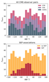 |
Fig. 1. Histogram of CME–observer pairs included in the study of > 10 MeV proton events versus Δϕ. (a): Stacked plot showing STEREO A, STEREO B, and GOES pairs. (b): Pairs without SEPs at the observer stacked on top of those with SEPs. Δϕ was calculated using the actual measured solar wind speed at the spacecraft. |
2.2. Occurrence distribution of proton SEP events
The bottom panel of Fig. 1 displays the subset of CME-observer pairs for which an SEP event was observed (144 pairs; red bars) over the histogram of all pairs (577 pairs; orange bars). Here it is evident that even for locations close to the ideal magnetic connection (Δϕ = 0) a significant number of events did not result in SEPs.
Comparing the points on the two sides of Δϕ = 0 (best possible magnetic connection to the source AR), an asymmetry is evident, with configurations with negative Δϕ more likely to result in the detection of an SEP event compared to those with a positive one. This asymmetry is not immediately visible in the related Δϕgeom histogram presented by Kihara et al. (2020), though it is present also in that plot (their Fig. 1b).
We explore the asymmetry in more detail in Fig. 2, which presents histograms of pairs for which SEPs were observed, for the case when Δϕ is calculated using (a) a constant vsw = 450 km s−1 and (b) the actual measured solar wind speed. Comparing the two panels one can see that using the actual vsw measured at the spacecraft produces a histogram that is more peaked around 0 and with a more pronounced lack of events for Δϕ > 40°.
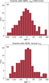 |
Fig. 2. Histogram of CME–observer pairs with SEPs observed, with Δϕ calculated using (a) an assumed vsw = 450 km s−1 and (b) the actual measured solar wind speed. |
A distribution of SEP detections can be obtained by dividing nSEP, the number of pairs with SEPs of Fig. 2b (using the actual vsw), by the total number npairs of CME-observer pairs in each bin (Fig. 1). The result is shown in Fig. 3. Error bars were calculated by assuming Poisson errors for nSEP and npairs and propagating the error to the ratio. The dashed yellow line is a Gaussian fit to the Δϕ < 0 portion of the histogram, mirrored to Δϕ > 0.
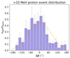 |
Fig. 3. Distribution in Δϕ of CME–observer pairs that resulted in SEPs being observed. The dashed line shows the Gaussian fit to the Δϕ < 0 portion of the histogram, mirrored to Δϕ > 0. |
Excluding the well-connected longitude range, defined here as the region where |Δϕ|< 40° (the four central bins in Fig. 3), there is a strong asymmetry in the Δϕ distribution of SEP event occurrence with respect to Δϕ = 0, with an excess of events in the negative side and a lack of events on the positive one. By summing nSEP/npairs for bins outside the well-connected region on each side of the histogram, we find that observers for which the source AR is on the eastern side of spacecraft footpoint are 93% more likely to detect an SEP event compared to observers with source AR on the western side. The mean of the distribution is  and its standard deviation is σΔϕ = 72°.
We tested the asymmetry of the SEP distribution in Fig. 3 by using a sign test. The sign test can be used to evaluate the null hypothesis that the distribution is symmetric with respect to a given Δϕ0, without making any assumptions on the shape of the distribution. Under the null hypothesis, the numbers of events with Δϕ < Δϕ0 and Δϕ > Δϕ0 follow a binomial distribution with a 50% probability that an event is at either side of Δϕ0. The statistical significance of the hypothesis can be evaluated with a standard binomial test. The sign test requires as input the number of events whereas the distribution in Fig. 3 represents the number of events per pair. We obtained the number of events by multiplying the values of nsep/npairs by the mean number of pairs per bin, obtained by averaging the histogram of Fig. 1. We used a one-sided sign test to assess whether the distribution in Fig. 3 is symmetric with respect to Δϕ0 = 0 and found that the null hypothesis can be rejected with a p-value of 0.038, showing that there is only a 3.8% probability that the null hypothesis is correct. Thus, the test implies there that the underlying distribution is asymmetric with respect to 0, with an excess of events for Δϕ < 0 compared to the Δϕ > 0 side. Based on the sign test, we conclude that the asymmetry with respect to Δϕ = 0 is statistically significant and SEP events are much more likely to be observed when the source AR is in the east with respect to the observer footpoint.
We further investigated the shape of the distribution. We calculated its Pearson-Fisher skewness parameter S, obtaining a value S = 0.40 (for comparison, the skewness of the half-normal distribution is 1). We compared the distribution to a normal distribution with the same mean  and sample standard deviation σΔϕ using a χ2 test, normalising both distributions to the representative event numbers using the same approach as for the sign test. We further summed bins where the representative count in the normalised normal distribution was smaller than 5, as small counts are known to give erroneous results within the χ2 test. We find that the null hypothesis of normality of the distribution cannot be rejected (p-value 0.63).
Therefore, the observed distribution is statistically compatible with an underlying Gaussian distribution peaking at  . Finally, we applied the sign test with Δϕ0 = −12° and found that the hypothesis of symmetry of the distribution with respect to the observed mean cannot be rejected (p-value 0.78). We note that the results of the statistical tests outlined above vary slightly depending on the exact Δϕ binning used; however, the conclusions remain unchanged irrespective of binning.
3. Electron events observed by MESSENGER
3.1. Electron dataset
Rodríguez-García et al. (2023a) carried out an extensive analysis of 61 solar energetic electron events detected by the MESSENGER spacecraft between 2010 and 2015. Events were identified using the 71–112 keV electron channel of the EPS instrument, part of the EPPS suite (Andrews et al. 2007). During the events, the spacecraft was located at heliocentric distances between 0.31 and 0.47 au. Of the 61 events, 57 were associated with a CME, as detailed in Rodríguez-García et al. (2023b).
Figure 1a of Rodríguez-García et al. (2023a) presents electron event peak intensity versus Δϕ, which they term connection angle, CA, defined as in Eq. (2): an E-W asymmetry in detection is visible in their plot. The asymmetry is explored further in our Fig. 4, which displays the histogram of the number of events versus Δϕ. Solar wind speed measurements are not available for MESSENGER therefore for the calculation of the spacecraft footpoint a solar wind speed vsw = 400 km s−1 was assumed, and the longitude of the source AR is that of the flare associated with the event (Rodríguez-García et al. 2023b). An asymmetry similar to that shown in Fig. 2 for protons can be seen. The total number of SEP events at MESSENGER is smaller than that of the proton events of Fig. 2, due to the high background of the MESSENGER particle instrument, as discussed in Rodríguez-García et al. (2023a), and the shorter time range.
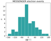 |
Fig. 4. Histogram of Δϕ values for the 61 MESSENGER electron events studied by Rodríguez-García et al. (2023a). The 71–112 keV electron channel was used to identify events. |
3.2. Occurrence distribution of electron SEP events
We derived an occurrence distribution of electron events versus Δϕ based on the dataset from Rodríguez-García et al. (2023a) using a methodology similar to that described in Sect. 2.2. Starting from the list of 239 CMEs from Kihara et al. (2020), we determined whether MESSENGER electron observations were available; this was the case for 208 CMEs, which we used for our analysis. For each one we calculated the value of Δϕ assuming a Parker spiral IMF. While the CMEs used in this analysis are the same as in Sect. 2, the Δϕ values for MESSENGER are different from those of the STEREO and GOES spacecraft. Figure 5a shows the distribution of Δϕ values for the CME-MESSENGER pairs. As was the case for the analysis in Sect. 2, there is fairly uniform coverage of the 360° around the Sun. We note that the bin centred at Δϕ = 75° shows a much larger number of CME events compared to the other bins.
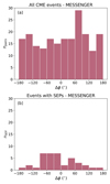 |
Fig. 5. Histogram of Δϕ values for (a) all CME events in the Kihara et al. (2020) dataset for which MESSENGER SEP observations were available and (b) a subset of events in (a) for which SEP electrons were observed (39 events). |
We then analysed whether an electron event took place at MESSENGER’s location in association with the CME event. Figure 5b shows the distribution in Δϕ of the events for which an SEP enhancement was detected. The number of events in this histogram is smaller than that of the histogram of Fig. 4 because not all the 61 SEP events of Fig. 4 have an associated CME that meets the selection criteria for inclusion in the Kihara et al. (2020) study (i.e. some have an associated CME with speed smaller than 900 km s−1 and angular width smaller than 60°).
By dividing the histogram of Fig. 5b by that of Fig. 5a, the distribution of events with SEPs shown in Fig. 6 was obtained. The total number of events is much smaller compared to the case of Fig. 3, due to the shorter time range over which MESSENGER data are available and the higher instrumental background. However, there are indications that the same detection asymmetry seen in the solar energetic proton event distribution is present also for electron events. It should be noted that despite the much larger number of CME events in the Δϕ = 75° bin compared to all the other bins, nSEP in this bin is low. Considering only configurations with |Δϕ|> 30°, events with negative Δϕ are 86% more likely than those with positive Δϕ. The mean of the distribution is  and its standard deviation is σΔϕ = 74°.
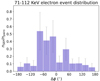 |
Fig. 6. Distribution in Δϕ of CME events that resulted in SEP electrons being observed by MESSENGER. |
Applying the sign test in a similar way as for the proton data, we found that the distribution in Fig. 6 is asymmetric with respect to Δϕ = 0 with p-value of 0.017. The null hypothesis (underlying distribution symmetric with respect to Δϕ = 0) has a probability of 1.7% and is thus rejected. Therefore, the detection asymmetry is present also in the electron data. The Pearson-Fisher skewness parameter for the distribution is S = 0.52. We could not perform a test of Gaussianity as the number of events is not sufficient for the χ2 test. Applying the sign test with respect to Δϕ0 = −18°, the assumption of symmetry with respect to the mean cannot be rejected (p-value 0.62).
4. Discussion
Indications that an E-W asymmetry in SEP event detection with respect to the best possible magnetic connection (Δϕ = 0) may be present in the data have been discussed in the literature. Kallenrode et al. (1992) presented an analysis of 77 SEP events detected by the Helios 1 and 2 spacecraft between 1974 and 1985. This dataset was affected by Earth bias in the flare observations but not the SEP observations. Their Fig. 4 displayed the distribution of the events in the Δϕ–heliolatitude plane: they noted an asymmetry in the E-W distribution of the events, with ∼2/3 lying in the Δϕ < 0 portion of the plane. They stated that this asymmetry had no physical reason and that they suspected it was due to the Helios orbit. They argued that events with large positive Δϕ would require the Helios spacecraft to be located behind the east limb and thus proposed that they may have been less numerous due to poor data transmission or radio blackouts (Kallenrode et al. 1992).
Dalla (2003) analysed 52 of the same SEP events (the subset of events identified as gradual) using data from Helios 1, Helios 2, and IMP8: they used 4–10 MeV and 28–36 MeV proton channels and the 0.7–2.0 MeV electron channel and plotted the duration of the SEP events versus Δϕ. The resulting graphs showed that events with large negative Δϕ tended to have the longest durations and those with large positive Δϕ had much shorter duration. They also considered the E-W asymmetry in event occurrence commented upon by Kallenrode et al. (1992) and carried out an analysis of the trajectories of the Helios 1 and 2 spacecraft: this showed that their orbits did not make events with large positive Δϕ less likely. They also pointed out that spacecraft–AR configurations leading to large positive Δϕ that did not involve the spacecraft being at risk of data transmission problems were possible. They thus termed this E-W asymmetry the ‘detection asymmetry’ and argued that it is a real physical effect.
He & Wan (2017) used a list of 78 major solar proton events at Earth from 1996–2011, produced by the NOAA Space Weather Prediction Centre, to show that, for |Δϕ|≲40°, there is an excess of events for negative Δϕ values compared to positive ones. This study is affected by Earth bias in flare observations since only observations of SEP source regions on the front side of the Sun were available in compiling the list (with a small fraction of the SEP events having been associated with regions that rotated over the west limb of the Sun). It is also affected by Earth bias in SEP observations as only near-Earth data were used. Thus, the study could not probe the 40° < Δϕ < 180° region. He & Wan (2017) ascribed the asymmetry to perpendicular diffusion effects.
The results presented in Sect. 2 are based on a much more extensive dataset compared to previous work and use, for the first time in this type of study, consistent information on solar sources of SEP events located on the far side of the Sun. In addition, by starting the analysis from a series of CME events, regardless of whether or not an SEP event was produced, we were able to derive distributions of occurrence of SEP events (Figs. 3 and 6). The proton distribution shows a clear E-W asymmetry in detection, confirming the earlier findings. The number of electron events from the MESSENGER dataset discussed in Sect. 3 is smaller than for protons, but a statistically significant asymmetry is present.
One limitation of our study is that it uses a high threshold to define an SEP proton event, because of the reliance on data from the GOES spacecraft, which has a high background. The MESSENGER electron instrument we utilised also has a high background, so a high threshold was again employed in the detection of electron events. Thus, the study has an overall emphasis on intense SEP events. The CME sample is focussed on fast and wide CMEs. It is hoped that future work will use different selection criteria and extend this type of study to other types of SEP and solar events.
Combining our proton and electron results with earlier indications of a similar asymmetry from data from the Helios 1 and Helios 2 spacecraft from 1974–1985 (Kallenrode et al. 1992; Dalla 2003), there are three independent datasets that probe large positive Δϕ values and confirm that the detection asymmetry in SEP events is a real effect. Our study shows that in the datasets we analysed the asymmetry arises despite the distribution of solar events with potential to produce SEPs being uniform in Δϕ. Thus, we conclude that the asymmetry in SEP event occurrence is real and it is caused by a physical effect.
One possible explanation for the E-W asymmetry in SEP detection is that it may be related to corotation of particle-filled magnetic flux tubes with the Sun. 3D test particle simulations have shown that corotation plays an important role in determining the characteristics of SEP events (Marsh et al. 2015; Dalla et al. 2017; Hutchinson et al. 2023). For an observing spacecraft for which the source AR is to the east of the magnetic footpoint (Δϕ < 0) corotation sweeps the magnetic field lines towards the observer, while if the source AR is to the west (Δϕ > 0), corotation takes magnetic flux tubes away from the observer. In the frame of reference of a magnetic flux tube corotating with the Sun, the particle flux evolves due to: (a) a time-dependent injection of accelerated particles directly into this tube and (b) the transport of particles in and out of the flux tube as a result of 3D effects. The latter may include perpendicular transport associated with turbulence (e.g. Strauss et al. 2017; Laitinen et al. 2023), guiding centre drifts (Dalla et al. 2013) and heliospheric current sheet drift (Waterfall et al. 2022). The SEP flux measured by an observer is the combined effect of time-dependent changes due to (a) and (b) within each flux tube, convolved with the spatial effect associated with corotation of the magnetic flux tubes themselves over the observer. Since detection of an SEP event requires the intensity to exceed the instrumental background of a given spacecraft detector (or, as in the present analysis, to cross a specified threshold), when the observer is not directly connected to the source region of the event it is reasonable to assume that, for Δϕ > 0 configurations, corotation works against intensities going above background at the observer, while for Δϕ < 0 it makes detection more likely by carrying magnetic flux tubes towards the observer. Hence, corotation may be a contributing factor to the observed E-W detection asymmetry. Because of the large variation in the magnitude and spatial extent of SEP events, it is still possible for events with large positive Δϕ to be detected; however, their detection is statistically less likely.
As a possible alternative explanation the observed asymmetry may be caused by a systematic E-W variation of efficiency of SEP energisation along an accelerating shock front (Cane et al. 1988; Tylka et al. 2005; Kahler 2016). Over time, a given observer is connected to different portions of a propagating CME-driven shock. Following on from ideas proposed by Sarris et al. (1984), Tylka et al. (2005) suggested that given that in part of its front the shock is quasi-parallel while in others it is quasi-perpendicular, the different efficiencies of acceleration for these two types of shock may explain differences in intensity profile parameters and composition. As noted by Kahler (2016) close to the Sun at the flanks of a CME shock there are no significant differences in shock obliquity between east and west. However, as the shock propagates farther from the corona, an observer with Δϕ > 0 will be connected to a quasi-parallel shock, while one with Δϕ < 0 to a quasi-perpendicular one. Thus, if what influences detection is acceleration far from the corona and acceleration at quasi-perpendicular shocks is more efficient, this may explain an asymmetry in detection. It should be noted that the above interpretation assumes a geometry of the CME shock where its flanks curve back towards the Sun, resulting in the quasi-parallel and quasi-perpendicular configurations, initially invoked by Sarris et al. (1984, see their Fig. 11) to explain features of SEP events. However, Cane (1988) argued that over an extent of approximately 120 degrees centred at the nose, the expansion speeds of a shock front tend to be similar, resulting in a shock geometry that is semi-circular. In this scenario the angle between shock normal and magnetic field does not vary strongly and the explanation above no longer holds. Ding et al. (2022) used a 2D model of SEP acceleration at a propagating CME shock to show that even a symmetric acceleration efficiency at the shock will result in an asymmetric injection with time since the shock connects to westward longitudes as it reaches larger radial distances.
A third possible explanation is that some asymmetry may be introduced by perpendicular diffusion processes during the transport of SEPs in the heliosphere (He & Wan 2017). Strauss et al. (2017) pointed out that the nature of diffusion perpendicular to the Parker spiral IMF produces a spatial distribution of SEP intensities in the heliosphere with peak located to the west of the best magnetic connection (see their Fig. 3), thus producing larger intensities for negative Δϕ (using the definition in Eq. (2)). The same feature can be observed in the spatial distributions from the model of Laitinen et al. (2023, see their Fig. 2). It is also possible that a combination of corotation, asymmetric SEP injection at a CME shock and interplanetary transport processes may contribute to the observed detection asymmetry.
The asymmetry in detection may be related to features in the distribution of SEP peak intensities that have been reported in the literature. Richardson et al. (2014) analysed individual three-spacecraft events by fitting a Gaussian to a plot of SEP peak intensity versus Δϕ at the three spacecraft. They found that there is a tendency for the location, Φ0, of the peak of the fitted Gaussian to be shifted towards negative Δϕ values (for the definition of Δϕ given in Eq. (2)). For 14–24 MeV protons they obtained Φ0 = −15 ± 35°. In an earlier study Lario et al. (2013) obtained Φ0 with a different methodology that uses simultaneous fitting of multiple events within the assumption that Φ0 and the width of the Gaussian are the same for all events. Rodríguez-García et al. (2023a) plotted electron peak intensities in the 71–112 keV channel versus Δϕ in their Fig. 1a and noted that peak intensities tended to be larger for negative Δϕ values.
Figure 7 shows SEP peak intensity Ip versus Δϕ for the > 10 MeV proton event dataset of Sect. 2: here one can see that outside of the well-connected range, Ip tends to be larger for the negative Δϕ range compared to the positive one. Therefore, the trend displayed in Fig. 7 agrees with that reported by Rodríguez-García et al. (2023a) for electrons. Given that event detection requires intensities to exceed a threshold (determined by either the instrumental background or the galactic cosmic ray intensity), if there is a tendency for events to be more intense in the negative Δϕ range compared to the positive one, this will produce a detection asymmetry such as the one we observed. In addition if the Ip versus Δϕ plot is as shown in Fig. 7 and reported in Rodríguez-García et al. (2023a), one would expect that for many three-spacecraft events the largest peak intensity is located at negative Δϕ values, resulting in the tendency for negative Φ0 values observed (Lario et al. 2013). Thus, the peak intensity trend observed causes the negative Φ0 values in three-spacecraft Gaussian fits. Therefore, we conclude that the underlying physics is likely the same for the detection asymmetry, the peak intensity asymmetry and the negative Φ0 Gaussian fit results. Corotation causes peak intensities to be larger for negative Δϕ because particle filled flux tubes corotate towards the observer, as shown by Hutchinson et al. (2023), and thus can explain the asymmetry in peak intensities. Strauss et al. (2017) ascribed the negative Φ0 Gaussian fit results to perpendicular diffusion, within a model that did not include corotation effects. Alternatively variation of acceleration efficiency along the shock could be causing the observed peak intensity trend.
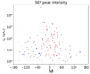 |
Fig. 7. SEP peak intensity versus Δϕ for the > 10 MeV proton events. Events with |Δϕ|< 40° are in red. |
Regarding the fact that both > 10 MeV proton and 71–112 keV electron data show indications of an E-W asymmetry in detection, it should be noted that the sources of SEP electrons and protons may be different and considerable debate exists in the literature on this point. Some electron events may have origin in localised regions, including flare reconnection regions. Within the corotation interpretation, however, regardless of the origin of the energetic particles, the magnetic flux tubes in which they are injected will be subject to rotation of the magnetic field lines and thus an asymmetry would be expected for both electrons and protons.
Test particle simulations of 5 MeV protons injected by a wide propagating shock-like source showed that, within an individual event, corotation results in a long-duration SEP decay phase at an observer with Δϕ < 0 (eastern AR with respect to the observer’s magnetic footpoint), while it contributes to the SEP event being ‘cut off’ for cases with Δϕ > 0 (western AR with respect to the footpoint; Hutchinson et al. 2023). They also demonstrated that, once corotation is included, the decay time constant of the event is independent of the scattering mean free path.
Hyndman et al. (2025) analysed the decay phase of SEP events and show that within individual events the decay time constant displays a systematic decrease with Δϕ: according to test particle simulations, this systematic behaviour is the result of corotation effects (Hutchinson et al. 2023). Thus, both detection asymmetry and analysis of SEP decay phases appear to point towards corotation playing an important role.
5. Conclusions
In this study we analysed the distribution of the occurrence of SEP events with respect to the connection angle, Δϕ, the longitude separation between the source AR location and the observer’s magnetic footpoint (Eq. (2)), using datasets that do not suffer from Earth bias. Our main conclusions are as follows:
-
Based on a dataset of 577 CME–observer pairs from 2006–2017 (Kihara et al. 2020), the distribution of occurrences of > 10 MeV proton SEP events at 1 au displays an E-W asymmetry with respect to Δϕ = 0. Outside the well-connected longitude range (i.e. for |Δϕ|> 40°), events with negative Δϕ are 93% more likely than those with positive Δϕ. Based on a sign test, the asymmetry is statistically significant; the null hypothesis (no asymmetry with respect to Δϕ = 0) has a probability of 3.8% and was thus rejected.
-
Occurrences of 71–112 keV electron SEP events measured by MESSENGER at radial distances between 0.31 and 0.47 au from 2010–2015 (Rodríguez-García et al. 2023a) also display a similar asymmetry, with a higher likelihood of events for negative Δϕ, though with lower total event numbers. A sign test rejects the null hypothesis (no asymmetry with respect to Δϕ = 0) since it has a probability of 1.7%.
As for Δϕ < 0, corotation sweeps particle-filled magnetic flux tubes towards the observer, and for Δϕ > 0 it moves them away, corotation as a spatial effect can provide an explanation for the observed asymmetry. Other effects such as E-W differences in the efficiency of acceleration at a CME-driven shock front or perpendicular transport effects are possible alternative explanations. It is interesting that the effect appears to be present for both electrons and protons, and is seen both close to the Sun (0.31–0.47 au) and at 1 au. The corotation explanation can account for these observations since corotation acts in the same way on protons and electrons and is present at both radial distances. We hope that future modelling will explore whether asymmetric acceleration at a CME shock or perpendicular transport can reproduce the observed features at various radial distances and for different species.
The distribution of event detections can be described either as characterised by an asymmetry with respect to Δϕ = 0 or as displaying a shift in its peak towards negative Δϕ values, with the mean of the distribution located at  for > 10 MeV protons and
  for 71–112 keV electrons. The physical mechanism responsible for these features is likely the same as for the asymmetry in the peak intensity distribution (Rodríguez-García et al. 2023a) and the offset in Gaussian fit peaks (Lario et al. 2013; Richardson et al. 2014).
Finally, if events with large positive Δϕ are much less likely, as our study indicates, this has potential consequences for space weather in terms of developing empirical tools and methodologies for SEP forecasting.
Acknowledgments
SD, TL and CW acknowledge support from the UK STFC (grants ST/V000934/1 and ST/Y002725/1) and NERC (via the SWARM project, part of the SWIMMR programme, grant NE/V002864/1). RH acknowledges support from a Moses Holden studentship. AH would like to acknowledge support from from STFC via a doctoral training grant, the University of Maryland Baltimore County (UMBC), the Partnership for Heliophysics and Space Environment Research (PHaSER), and NASA/GSFC. NVN has been supported by NASA grant 80NSSC24K0175. L.R.-G. acknowledges support through the European Space Agency (ESA) research fellowship programme. CW’s research is supported by the NASA Living with a Star Jack Eddy Postdoctoral Fellowship Program, administered by UCAR’s Cooperative Programs for the Advancement of Earth System Science (CPAESS) under award #80NSSC22M0097[1]. Data Access Statement: The datasets used in this paper are publicly available as follows. The CME event and SEP proton enhancement dataset used in Section 2 has been published in Kihara et al. (2020), with their Table 1 providing all the relevant data. The electron SEP event dataset used for the analysis of Section 3 has been published in Rodríguez-García et al. (2023a) in their Appendix A, Table A.1.
References
- Andrews, G. B., Zurbuchen, T. H., Mauk, B. H., et al. 2007, Space Sci. Rev., 131, 523 [CrossRef] [Google Scholar]
- Brueckner, G. E., Howard, R. A., Koomen, M. J., et al. 1995, Sol. Phys., 162, 357 [NASA ADS] [CrossRef] [Google Scholar]
- Burlaga, L. F. 1967, J. Geophys. Res., 72, 4449 [NASA ADS] [Google Scholar]
- Cane, H. V. 1988, J. Geophys. Res., 93, 1 [NASA ADS] [Google Scholar]
- Cane, H. V., Reames, D. V., & von Rosenvinge, T. T. 1988, J. Geophys. Res., 93, 9555 [NASA ADS] [CrossRef] [Google Scholar]
- Cohen, C. M. S., Mason, G. M., & Mewaldt, R. A. 2017, ApJ, 843, 132 [NASA ADS] [CrossRef] [Google Scholar]
- Cohen, C. M. S., Li, G., Mason, G. M., Shih, A. Y., & Wang, L. 2021, in Solar Physics and Solar Wind, eds. N. E. Raouafi, & A. Vourlidas, 1, 133 [NASA ADS] [CrossRef] [Google Scholar]
- Dalla, S. 2003, in Solar Wind Ten, eds. M. Velli, R. Bruno, F. Malara, & B. Bucci, Am. Inst. Phys. Conf. Ser., 679, 660 [NASA ADS] [CrossRef] [Google Scholar]
- Dalla, S., Marsh, M. S., Kelly, J., & Laitinen, T. 2013, J. Geophys. Res. (Space Phys.), 118, 5979 [NASA ADS] [CrossRef] [Google Scholar]
- Dalla, S., Marsh, M. S., & Battarbee, M. 2017, ApJ, 834, 167 [NASA ADS] [CrossRef] [Google Scholar]
- Desai, M., & Giacalone, J. 2016, Liv. Rev. Sol. Phys., 13, 3 [NASA ADS] [CrossRef] [Google Scholar]
- Ding, Z., Li, G., Ebert, R. W., et al. 2022, J. Geophysical Res. (Space Phys.), 127, e30343 [NASA ADS] [Google Scholar]
- Domingo, V., Fleck, B., & Poland, A. I. 1995, Sol. Phys., 162, 1 [Google Scholar]
- Dröge, W., Kartavykh, Y. Y., Klecker, B., & Kovaltsov, G. A. 2010, ApJ, 709, 912 [CrossRef] [Google Scholar]
- Forsyth, R. J., & Gosling, J. T. 2001, in The Heliosphere Near Solar Minimum. The Ulysses Perspective, eds. A. Balogh, R. G. Marsden, & E. J. Smith (Springer), 107 [Google Scholar]
- Giacalone, J., & Jokipii, J. R. 2012, ApJ, 751, L33 [NASA ADS] [CrossRef] [Google Scholar]
- He, H.-Q., & Wan, W. 2017, MNRAS, 464, 85 [NASA ADS] [CrossRef] [Google Scholar]
- Heber, B., Sanderson, T. R., & Zhang, M. 1999, Adv. Space Res., 23, 567 [NASA ADS] [Google Scholar]
- Hutchinson, A., Dalla, S., Laitinen, T., & Waterfall, C. O. G. 2023, A&A, 670, L24 [NASA ADS] [CrossRef] [EDP Sciences] [Google Scholar]
- Hyndman, R. A., Dalla, S., Laitinen, T., et al. 2025, A&A, 694, A242 [NASA ADS] [CrossRef] [EDP Sciences] [Google Scholar]
- Kahler, S. W. 2016, ApJ, 819, 105 [NASA ADS] [CrossRef] [Google Scholar]
- Kaiser, M. L., Kucera, T. A., Davila, J. M., et al. 2008, Space Sci. Rev., 136, 5 [Google Scholar]
- Kallenrode, M.-B., & Wibberenz, G. 1997, J. Geophys. Res., 102, 22311 [NASA ADS] [CrossRef] [Google Scholar]
- Kallenrode, M. B., Cliver, E. W., & Wibberenz, G. 1992, ApJ, 391, 370 [NASA ADS] [CrossRef] [Google Scholar]
- Kihara, K., Huang, Y., Nishimura, N., et al. 2020, ApJ, 900, 75 [NASA ADS] [CrossRef] [Google Scholar]
- Klein, K.-L., & Dalla, S. 2017, Space Sci. Rev., 212, 1107 [Google Scholar]
- Laitinen, T., Dalla, S., Battarbee, M., & Marsh, M. S. 2018, in Space Weather of the Heliosphere: Processes and Forecasts, eds. C. Foullon, & O. E. Malandraki, IAU Symp., 335, 298 [NASA ADS] [Google Scholar]
- Laitinen, T., Dalla, S., Waterfall, C. O. G., & Hutchinson, A. 2023, A&A, 673, L8 [NASA ADS] [CrossRef] [EDP Sciences] [Google Scholar]
- Lario, D., Aran, A., Gómez-Herrero, R., et al. 2013, ApJ, 767, 41 [CrossRef] [Google Scholar]
- Lario, D., Sanahuja, B., & Heras, A. M. 1998, ApJ, 509, 415 [NASA ADS] [CrossRef] [Google Scholar]
- Marsh, M. S., Dalla, S., Dierckxsens, M., Laitinen, T., & Crosby, N. B. 2015, Space Weather, 13, 386 [CrossRef] [Google Scholar]
- Mewaldt, R. A., Cohen, C. M. S., Cook, W. R., et al. 2008, Space Sci. Rev., 136, 285 [Google Scholar]
- Odstrcil, D., & Pizzo, V. J. 1999, J. Geophys. Res., 104, 28225 [NASA ADS] [CrossRef] [Google Scholar]
- Onsager, T., Grubb, R., Kunches, J., et al. 1996, in GOES-8 and Beyond, ed. E. R. Washwell, SPIE, 2812, 281 [NASA ADS] [CrossRef] [Google Scholar]
- Owens, M. J., Challen, R., Methven, J., Henley, E., & Jackson, D. R. 2013, Space Weather, 11, 225 [CrossRef] [Google Scholar]
- Owens, M., Lang, M., Barnard, L., et al. 2020, Sol. Phys., 295, 43 [NASA ADS] [CrossRef] [Google Scholar]
- Papaioannou, A., Sandberg, I., Anastasiadis, A., et al. 2016, J. Space Weather Space Clim., 6, A42 [NASA ADS] [CrossRef] [EDP Sciences] [Google Scholar]
- Pesnell, W. D., Thompson, B. J., & Chamberlin, P. C. 2012, Sol. Phys., 275, 3 [Google Scholar]
- Pomoell, J., & Poedts, S. 2018, J. Space Weather Space Clim., 8, A35 [NASA ADS] [CrossRef] [EDP Sciences] [Google Scholar]
- Richardson, I. G., von Rosenvinge, T. T., Cane, H. V., et al. 2014, Sol. Phys., 289, 48 [NASA ADS] [Google Scholar]
- Rodríguez-García, L., Balmaceda, L. A., Gómez-Herrero, R., et al. 2023a, A&A, 674, A145 [NASA ADS] [CrossRef] [EDP Sciences] [Google Scholar]
- Rodríguez-García, L., Gómez-Herrero, R., Dresing, N., et al. 2023b, A&A, 670, A51 [NASA ADS] [CrossRef] [EDP Sciences] [Google Scholar]
- Sarris, E. T., Anagnostopoulos, G. C., & Trochoutsos, P. C. 1984, Sol. Phys., 93, 195 [NASA ADS] [Google Scholar]
- Solomon, S. C., McNutt, R. L., Gold, R. E., & Domingue, D. L. 2007, Space Sci. Rev., 131, 3 [NASA ADS] [CrossRef] [Google Scholar]
- Strauss, R. D. T., Dresing, N., & Engelbrecht, N. E. 2017, ApJ, 837, 43 [NASA ADS] [CrossRef] [Google Scholar]
- Tylka, A. J., Cohen, C. M. S., Dietrich, W. F., et al. 2005, ApJ, 625, 474 [NASA ADS] [CrossRef] [Google Scholar]
- Van Hollebeke, M. A. I., Ma Sung, L. S., & McDonald, F. B. 1975, Sol. Phys., 41, 189 [Google Scholar]
- von Rosenvinge, T. T., Reames, D. V., Baker, R., et al. 2008, Space Sci. Rev., 136, 391 [Google Scholar]
- Waterfall, C. O. G., Dalla, S., Laitinen, T., Hutchinson, A., & Marsh, M. 2022, ApJ, 934, 82 [NASA ADS] [CrossRef] [Google Scholar]
- Whitman, K., Egeland, R., Richardson, I. G., et al. 2023, Adv. Space Res., 72, 5161 [NASA ADS] [CrossRef] [Google Scholar]
- Wuelser, J. P., Lemen, J. R., Tarbell, T. D., et al. 2004, in Telescopes and Instrumentation for Solar Astrophysics, eds. S. Fineschi, & M. Gummin, SPIE Conf. Ser., 5171, 111 [NASA ADS] [CrossRef] [Google Scholar]
All Figures
|
Fig. 1. Histogram of CME–observer pairs included in the study of > 10 MeV proton events versus Δϕ. (a): Stacked plot showing STEREO A, STEREO B, and GOES pairs. (b): Pairs without SEPs at the observer stacked on top of those with SEPs. Δϕ was calculated using the actual measured solar wind speed at the spacecraft. |
| In the text | |
|
Fig. 2. Histogram of CME–observer pairs with SEPs observed, with Δϕ calculated using (a) an assumed vsw = 450 km s−1 and (b) the actual measured solar wind speed. |
| In the text | |
|
Fig. 3. Distribution in Δϕ of CME–observer pairs that resulted in SEPs being observed. The dashed line shows the Gaussian fit to the Δϕ < 0 portion of the histogram, mirrored to Δϕ > 0. |
| In the text | |
|
Fig. 4. Histogram of Δϕ values for the 61 MESSENGER electron events studied by Rodríguez-García et al. (2023a). The 71–112 keV electron channel was used to identify events. |
| In the text | |
|
Fig. 5. Histogram of Δϕ values for (a) all CME events in the Kihara et al. (2020) dataset for which MESSENGER SEP observations were available and (b) a subset of events in (a) for which SEP electrons were observed (39 events). |
| In the text | |
|
Fig. 6. Distribution in Δϕ of CME events that resulted in SEP electrons being observed by MESSENGER. |
| In the text | |
|
Fig. 7. SEP peak intensity versus Δϕ for the > 10 MeV proton events. Events with |Δϕ|< 40° are in red. |
| In the text | |
Current usage metrics show cumulative count of Article Views (full-text article views including HTML views, PDF and ePub downloads, according to the available data) and Abstracts Views on Vision4Press platform.
Data correspond to usage on the plateform after 2015. The current usage metrics is available 48-96 hours after online publication and is updated daily on week days.
Initial download of the metrics may take a while.