| Issue |
A&A
Volume 670, February 2023
|
|
|---|---|---|
| Article Number | A178 | |
| Number of page(s) | 12 | |
| Section | The Sun and the Heliosphere | |
| DOI | https://doi.org/10.1051/0004-6361/202245313 | |
| Published online | 24 February 2023 | |
Modelling shock-like injections of solar energetic particles with 3D test particle simulations
Jeremiah Horrocks Institute, University of Central Lancashire, Preston PR1 2HE, UK
e-mail: This email address is being protected from spambots. You need JavaScript enabled to view it.
Received:
28
October
2022
Accepted:
30
December
2022
Abstract
Context. Solar energetic particle (SEP) acceleration and injection into interplanetary space during gradual SEP events is thought to take place at coronal mass ejection (CME)-driven shocks. Various features of measured intensity profiles at 1 au have been attributed to properties of the radial, longitudinal, and latitudinal SEP injections at the shock. Focussed transport models are typically used to model acceleration at a CME-shock and subsequent propagation. Test particle simulations are an alternative approach but so far they have been carried out only with instantaneous injection near the Sun.
Aims. We develop the first temporally extended shock-like injection for our 3D test particle code and investigate how the spatial features of injection at a shock affect SEP intensity and anisotropy profiles for observers at 0.3 and 1.0 au.
Methods. We conducted simulations of a monoenergetic population of 5 MeV protons considering three different radial injection functions and two longitudinal and latitudinal injection functions. We considered a range of scattering conditions with scattering mean free path values ranging from λ = 0.1 − 1.0 au, and determined intensity and anisotropy profiles at six observers at different longitudinal locations.
Results. We find that the radial, longitudinal, and latitudinal injection functions play a relatively minor role in shaping the SEP intensity profiles. The dependence of intensity profiles on the value of the scattering mean free path is also weak, unlike what is found from 1D focussed transport models. Spatial factors, such as the times of observer-shock connection and disconnection as well as the time of shock passage have a much stronger influence on SEP intensities and anisotropies. Persistent anisotropies, until shock passage, are seen in our simulations. Comparing instantaneous and shock-like injections, we find that the link between the duration of injection and the duration of the SEP event is very weak, unlike what is commonly assumed.
Key words: Sun: coronal mass ejections (CMEs) / Sun: particle emission
© The Authors 2023
 Open Access article, published by EDP Sciences, under the terms of the Creative Commons Attribution License (https://creativecommons.org/licenses/by/4.0), which permits unrestricted use, distribution, and reproduction in any medium, provided the original work is properly cited.
This article is published in open access under the Subscribe to Open model. This email address is being protected from spambots. You need JavaScript enabled to view it. to support open access publication.
1. Introduction
Gradual solar energetic particle (SEP) events are enhancements in energetic ions and electrons in the interplanetary medium, observed in association with solar flares and coronal mass ejections (CMEs). They are often found to have a long duration (e.g., several days) and wide longitudinal extent (e.g., > 80°), as evidenced by multi-spacecraft observations (e.g., Desai & Giacalone 2016, and references therein).
Gradual events are thought to originate at CME-driven shocks, with particle acceleration taking place over extended times as the shock propagates though the corona and interplanetary space. Several properties of the SEP intensity profiles have been linked to properties of the shock acceleration. It is thought that the characteristic long duration decays measured by spacecraft at 1 au (Cane et al. 1988) are caused by the fact that CME-shock acceleration is extended in time (Reames et al. 1997). In addition, the dependence of the overall shape of SEP intensity profiles on the location of the associated solar active region, AR (east-west effect, Cane et al. 1988), has been attributed to the longitudinal variation of efficiency across the shock front (e.g., Tylka & Lee 2006; Zank et al. 2006).
A number of models have studied SEP acceleration and injection at CME-driven shocks with the purpose of deriving observables at 1 au, and determining the main physical processes that influence them. Several studies have modelled shock-like injections and the subsequent propagation of SEPs using particle transport equations (e.g., Kallenrode & Wibberenz 1997; Lario et al. 1998; He et al. 2011; Wang et al. 2012; Qin et al. 2013).
Kallenrode & Wibberenz (1997) used a black box shock model, and solved the 1D focussed transport equation to produce intensity and anisotropy profiles for a variety of particle injection and propagation parameters. Lario et al. (1998) modelled SEP events with an improved transport equation that considered solar wind convection and adiabatic deceleration, and used a magnetohydrodynamic (MHD) model to derive the shock propagation. They fitted observed particle flux and anisotropy profiles for four particle events and found that the efficiency of the shock as a particle accelerator decreases rapidly with distance from the Sun for particle energies greater than ∼2 MeV. Heras et al. (1994) emphasised the importance of the geometry of magnetic connection between the shock and the observer in determining features of SEP intensity profiles, and stressed the importance of the time evolution of magnetic connection to the shock.
As an alternative to focussed transport models, full-orbit test-particle simulations of SEP propagation calculate individual particle trajectories throughout the heliosphere by solving the particle’s equation of motion. These types of simulations are intrinsically 3D. Previously, we used test particle simulations to study propagation through the interplanetary magnetic field for the case of instantaneous particle injections close to the Sun (e.g., Marsh et al. 2015; Battarbee et al. 2018; Dalla et al. 2020; Waterfall et al. 2022). Hutchinson et al. (2022) used instantaneous particle injections at a range of heights in the solar atmosphere to study proton back-precipitation to the photosphere.
In this paper we present results from 3D test particle simulations in which, for the first time, particle injection is from a moving shock-like source. This means that it is spatially extended over a wide shock and temporally extended since particles keep being injected as the shock propagates though the heliosphere. This new injection considers a simple model of a shock, similar to that developed by Heras et al. (1994) and Kallenrode & Wibberenz (1997), and it provides a first step in accounting for temporally extended particle injections in 3D full orbit test particle simulations.
We investigate the effect of choosing different radial and angular injection profiles on the intensity and anisotropy profiles at 1 au at different observers. We study the effect of a variety of interplanetary scattering conditions on observables. We compare intensity and anisotropy profiles for observers at 0.3 and 1.0 au, to provide comparisons with Parker Solar Probe and Solar Orbiter observations. In a companion paper (Hutchinson et al. 2023), a comparison between simulations that do and do not include the corotation of magnetic flux tubes is presented. The layout of the paper is as follows: in Sect. 2 we describe the shock-like injection. In Sect. 3 we explore its implementation within 3D test particle simulations. In Sect. 4 we describe the geometry of the observers. Intensity and anisotropy profiles are investigated for a variety of shock-like injections and scattering parameters in Sect. 5. A discussion and conclusions can be found in Sect. 6.
2. Shock-like injection model
We have developed a particle injection model that approximates a temporally extended injection from a propagating shock-like source (referred to as the shock in the following), which is of constant angular width in longitude and latitude. The injection is spatially extended across the shock front and temporally extended, occurring over timescales of days as the shock propagates radially outwards. Our simplified description accounts for the geometric characteristics of the shock injection and its evolution with time, but it neither models acceleration nor the evolution of the shock as an MHD structure. We note that the shock has a negligible thickness within the model.
We used a spherical coordinate system (r, θ, ϕ) where r is the radial distance from the centre of the Sun, θ is heliographic colatitude, and ϕ is heliographic longitude with corresponding unit vectors  ,
,  , and
, and  . The shock is assumed to propagate with a constant speed, vsh, and maintain the same angular width in longitude and latitude as it propagates. Particle injection is assumed to continue as the shock propagates through the corona and interplanetary space, taking place over r ∈ [rmin, rmax], where rmin and rmax are the minimum and maximum particle injection radii. We chose rmin = 1.2 R⊙, the median shock formation height as determined by Gopalswamy (2013).
The shock in the model acts only as a particle source and does not interact with or modify the interplanetary magnetic field (IMF), which is assumed to be a Parker spiral (Eq. (14)). Particles were injected isotropically from the shock surface throughout its propagation, consistent with theories of diffusive shock acceleration (Baring 1997; Desai & Giacalone 2016). The shock is effectively transparent to particles, meaning any particle that returns to the shock position during its propagation does not interact with it and travels straight through, without a change to its trajectory.
Table 1 summarises the shock parameters and gives the typical values used in our simulations unless otherwise stated. We define wsh, ϕ as the longitudinal width of the shock, wsh, θ as the colatitudinal width, and δcent as the latitude of the centre of the shock (where δ = 90° −θ is latitude). In the majority of our simulations, we chose wsh, ϕ = wsh, θ = 70°, purely radial shock speed vsh = 1500 km s−1, and we assumed that particle acceleration and injection take place over a period of two days, resulting in rmax = 372 R⊙(=1.73 au). The shock is centred at ϕcent = 0° and latitude δcent = 15°, so as to represent the typical CME latitudes, corresponding to the positions of the activity belts on the solar disc.
Parameters of shock-like injection and in our test particle simulations.
2.1. Particle injection and normalisation
We introduce a function S(r, θ, ϕ) describing the number of particles per unit volume injected by the shock at position (r, θ, ϕ), so that
 (1)
(1)
with Np being the total number of particles and d3r the unit volume. Here the dependence on time is folded into the radial dependence via r = vsht.
We assume that S is separable, so that
 (2)
(2)
where R(r), Φ(ϕ), and Θ(θ) are the radial, longitudinal, and colatitudinal injection functions, respectively, satisfying the following normalisation conditions:
 (3)
(3)
 (4)
(4)
 (5)
(5)
2.2. Radial injection function
In our model we considered a number of radial injection functions. The simplest radial injection function is R(r) = const, the uniform case, where the shock injects the same number of particles as r increases. The normalisation condition for the uniform case gives the following:
 (6)
(6)
We note that as the shock propagates to larger radial positions with a fixed angular width, the surface area of the shock increases as r2. Therefore, for uniform R(r), (Eq. (6)), the number of particles injected per unit area of the shock, Q(r), decreases with r as 1/r2 (see Fig. 1 bottom panel).
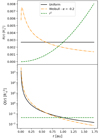 |
Fig. 1. Radial injection function, R(r) vs. r (top), and the number of particles injected per unit area of the shock, Q(r) vs. r (bottom). |
We also considered a non-uniform injection given by the modified Weibull function (previously used to describe SEP profiles by Kahler & Ling 2018). Normalised over our injection range, this is given by
 (7)
(7)
where α (α < 0) and β are parameters that determine the shape of the function, specifically the rise and decay rates and the position of the peak. We chose rpeak = 5 R⊙, which results in a fast rise phase near the Sun and a decay phase beyond 5 R⊙. The Weibull function is plotted in orange in Fig. 1 (top panel).
To study the case of constant injection per unit area of the shock, we also considered a radial injection function proportional to r2. This function is described by
 (8)
(8)
The number of injected particles per unit area of the shock is
 (9)
(9)
where A(r) is the surface area of the shock front at a given radial position, given by
 (10)
(10)
Figure 1 (top) displays all radial injection functions, R(r) vs. the radial shock position, and Fig. 1 (bottom) displays the corresponding Q(r).
2.3. Longitudinal and latitudinal injection functions
We considered two types of injection efficiency with respect to the longitudinal and latitudinal position across the shock front. The first is uniform injection efficiency across the shock front, described by the following normalised expressions:
 (11)
(11)
 (12)
(12)
The second longitudinal and latitudinal injection function is a Gaussian centred about the shock nose. Typically we considered standard deviations of σϕ (σθ) = wsh, ϕ/4 (wsh, θ/4). The two injection functions are displayed in Fig. 2 for the longitudinal injection efficiency.
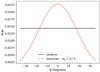 |
Fig. 2. Longitudinal injection function, Φ(ϕ), for the shock-like injection. |
3. 3D full-orbit test particle simulations
We modelled SEP propagation using a 3D full-orbit test particle code, originally developed by Dalla & Browning (2005), that has since been adapted to model various aspects of SEP propagation (e.g., Marsh et al. 2013; Battarbee et al. 2018). The model calculates particle trajectories by integrating their equation of motion,
 (13)
(13)
where p is the particle momentum, c is the speed of light, t is time, q is the charge of the particle, m0 is the particle rest mass, γ is the Lorentz factor, and E and B are the electric and magnetic fields, respectively.
Within this model, we considered a Parker spiral magnetic field described by
 (14)
(14)
where B0 is the magnetic field strength at a fixed reference radial distance r0, Ω is the sidereal solar rotation rate, and vsw is the solar wind speed. For our simulations we considered a unipolar positive magnetic field (i.e., oriented antisunwards) and solar wind speed of 500 km s−1 (same parameter values as Marsh et al. 2013). An electric field is present in the non-rotating (spacecraft) coordinate system due to the outward flow of the solar wind, and it is defined by the following (Marsh et al. 2013; Dalla et al. 2013):
 (15)
(15)
Its effect on the particle trajectories is to make particles corotate with the magnetic flux tubes in which they propagate. Hence corotation effects were included in our simulations. Within the model we considered the effects of magnetic turbulence by introducing pitch angle scattering, characterised by a mean free path λ. For further details on the scattering model, readers can refer to Marsh et al. (2013) and Dalla et al. (2020).
We note that in this first study of the effects of time-extended injection, our model does not include the effects of turbulence-associated perpendicular diffusion, which would affect the intensity profiles observed at different longitudinal positions, as shown by Wang et al. (2012). However, the addition of perpendicular diffusion will be the subject of further studies.
We considered pitch-angle scattering mean free paths in the range λ = 0.1–1.0 au and simulated particle propagation for three days with injection occurring over the first two days from the shock-like source. We considered a monoenergetic population of 5 MeV protons. In each simulation we injected Np = 106 particles. An isotropic velocity distribution at injection was assumed. While in our previous modelling work particles were injected into the simulation at t = 0 and close to the Sun (instantaneous injection), for this study we used the model of shock-like injection described in Sect. 2 to start particles at a distance r and t = r/vsh.
4. Geometry of observers
We derived observables at six observers (labelled A-F) located at 1 au, which can be seen in Fig. 3, describing the observer-shock geometry at four snapshots in time. In Fig. 3 the orange arrow gives the longitude of the shock nose, coincident with the active region (AR) longitude on the Sun, and the thin grey curved lines show the range of flux tubes that have been filled with particles by the shock up to time t. The solid green lines delimit the longitudinal range of IMF lines that are connected to the shock at the initial time (or an instantaneous injection at the Sun with the same angular width), and the red solid curved lines show the range of IMF lines connected to the shock front at the current time.
 |
Fig. 3. Diagrams showing the shock position and observer geometry at t = 0 (top left), 16 (top right), 32 (bottom left), and 48 (bottom right) hours projected onto the solar equatorial plane. Here x and y are heliocentric Cartesian coordinates in the heliographic equatorial plane. The shock’s projection onto the plane is displayed here as the orange shaded segments. Observers A-F are denoted by the coloured circles, and their exact positions are displayed in Table 2. The red radial dashed lines delimit the bounds of the shock, and the solid red curved lines show the IMF lines that are currently connected to the flanks of the shock front. The solid green curved lines show the bounds of the shock-like injection at the initial time (or equally an instantaneous injection at the Sun of the same angular width). The dashed green line shows the original position of the left most solid green line at the initial time. The grey IMF lines represent the range of IMF lines that have had particles injected onto them (the particle-filled flux tubes). |
The AR is located at (0° ,15°) longitude and latitude, respectively. As specified in Table 2, observers A, B, and C observe the AR as being western, while observers D, E, and F observe it as being eastern. Observers C and D are in the path of the shock and will observe it as it passes them, while the other observers will not experience the shock passage in situ. All observers are located at δ = 15° latitude to enable connection to the nose of the shock. We have examined the intensity profiles for observers at the same longitudes and at latitude δ = 0° and there are only very minor differences compared to the plots for δ = 15°, shown in Sect. 5.
We define the longitudinal separation between the AR and the observer footpoint, Δϕ, as
 (16)
(16)
where ϕAR is the longitudinal position of the source AR on the Sun and ϕftpt is the longitude of the footpoint of the IMF line connected to the observer. Values of Δϕ for our observers are given in Table 2.
An observer’s connection to the shock evolves over time. The observer’s cobpoint, where the observer’s IMF line meets the shock, moves eastwards along the shock front as the shock propagates outwards (e.g., Heras et al. 1994; Kallenrode & Wibberenz 1997).
5. Intensity time profiles and anisotropies
From the output of our test particle simulations, we have calculated observables such as intensity profiles and anisotropies for our observers under a number of conditions. Particle counts at each observer were collected over a 10° ×10° tile in longitude and latitude. Particle anisotropy, A, was calculated at each observer using the following equation (e.g., Kallenrode & Wibberenz 1997):
 (17)
(17)
where f(μ) is the pitch angle distribution and μ is the pitch angle cosine. We note that the sign of the anisotropy is dependent on the magnetic polarity: in the following we use a unipolar antisunward magnetic field in which case positive anisotropy represents antisunward propagating particles. For this polarity according to Eq. (17), an anisotropy of three corresponds to a fully beamed population travelling along the IMF antisunwards.
5.1. Effect of scattering mean free path on intensity and anisotropy profiles
We begin by analysing intensities and anisotropies at observers A–F under a variety of scattering conditions. Here we consider uniform injection in r, θ, and ϕ. In Fig. 4 we display the intensity and anisotropy profiles for the six observers, for simulations with a mean free path spanning an order of magnitude from λ = 0.1 to 1.0 au.
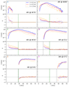 |
Fig. 4. Intensity profiles of a monoenergetic population of 5 MeV protons for observers A–F at 1.0 au for a range of scattering conditions from λ = 0.1 au to λ = 1.0 au, for uniform injection in r, θ, and ϕ. The green dashed line indicates the time at which the shock reaches the observer radial distance, and the vertical dotted line shows the time when the observer establishes connection to the shock, for observers not connected at the initial time. |
In Fig. 4 intensity profiles for different λ values at each observer appear remarkably similar to each other. In contrast to what has been derived from traditional 1D focussed transport models (e.g., Bieber et al. 1994), we do not see a significant change in the decay time constants with λ. SEPs in simulations with larger λ stream out more quickly. As expected for larger λ, we find smaller peak intensities and larger anisotropies, due to fewer scattering events.
The broad features of the intensity profiles at the six observers can be understood in terms of the geometry of the observers relative to the shock. As seen in Fig. 3a, observers A, B, and C are connected to the shock at the initial time. As the shock propagates outwards, their cobpoints fall off the eastern edge of the shock, losing connection to the particle source (see Fig. 3d for observer A). Over time, the shock connects to longitudes further west and allows observers D, E, and F to become connected to the shock source (e.g., Heras et al. 1994). This enables observers D, E, and F, which are not initial magnetically connected to the shock, to observe SEPs once connection is established. The intensity profiles in Fig. 4 reflect the different timings of the observer-shock connection, with the onset of the event being delayed at observers D–F.
In Fig. 4 the bottom panels display the anisotropy profiles observed at each of the six observers. The anisotropies clearly indicate the times of observer-shock connection. In Fig. 4 the vertical green line shows the time of shock arrival at the observer’s radial distance and the vertical black dotted line indicates the nominal time of observer-shock connection, for the observers not connected at the initial time. For observers C and D, sustained long-duration anisotropies are observed until the time of shock passage, in agreement with previous studies (e.g., Kallenrode & Wibberenz 1997; Kallenrode 2001). Observers E and F become connected to the shock when it is located beyond the observer radial position, and so they see negative anisotropies due to the sunward propagating particles from the shock.
Observers C and D see the peak intensity at the time of shock passage. Once the shock propagates past these observers, they are receiving sunward propagating particles injected at the shock and particles that were previously injected into the flux tube and have experienced scattering. As the shock propagates beyond the observer, the intensity of the former component diminishes with time as particles must overcome the magnetic mirror effect to reach the observer (e.g., Klein et al. 2018; Hutchinson et al. 2022). As a result, after shock passage, the anisotropies drop to zero, similar to the results of Kallenrode & Wibberenz (1997).
The peak intensities for observers A and B coincide with their loss of connection to the shock front due to corotation and shock radial motion (i.e., the observer’s cobpoint falls off the eastern edge of the shock front). These geometric effects are highly dependent on parameters such as the shock longitudinal width, wsh, ϕ, the radial speed of the shock, and the observer longitudinal position relative to the edge of the shock front. Hutchinson et al. (2023) compared observables for the cases with and without corotation included, and they have demonstrated that corotation plays a major role in the decay phase of the event.
5.2. Time-extended versus instantaneous injection
In previous work with our test-particle model, we only considered an instantaneous injection close to the Sun. We now compare observables for the cases of instantaneous injection and a radially uniform time-extended shock-like injection. We considered an instantaneous injection that has the same angular width as the extended injection (70° ×70°). The intensity profiles for the two cases can be seen in Fig. 5 for simulations considering λ = 0.1 au, where the solid black line is the radially uniform shock-like injection and the blue dashed line is the instantaneous injection. The same number of particles were injected into each simulation resulting in a significantly larger particle density close to the Sun for the instantaneous injection. This leads to systematically larger intensities for well-connected observers for the instantaneous injection (observers A–C). From the first panel (Observer A,) it can be seen that both the time-extended and instantaneous injection lead to the same event duration (∼12 h). This occurs as the corotation sweeps the particle-filled flux tubes westwards and away from the observer. Similarly, for observer B the intensity profile is cut short by the corotation. The corotation enables observer D to see a signal from the instantaneous injection as the particle-filled flux tubes corotate to this observer. In the shock-like simulations, observer D detects SEPs from the CME-driven shock approximately 10 h earlier compared to the instantaneous injection, showing the clear timescale differences between the two cases. Observers E and F do not receive particles from the instantaneous injection over the timescales of our simulations as the corotation takes longer than 72 h to rotate the particle-filled flux tubes to these observers. From Fig. 5 it is clear that a temporally extended injection does not necessarily mean a longer duration SEP event, especially for western events.
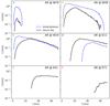 |
Fig. 5. Intensity profiles for observers A–F considering an instantaneous injection (blue dashed lines) and an extended uniform injection (solid black lines) with respect to r, θ, and ϕ. The injection region is 70° in both cases. The simulations use λ = 0.1 au. |
5.3. Dependence on the radial injection function
In Fig. 6 we consider three radial injection functions (uniform, Weibull, and r2, see Fig. 1) and determine the intensity profiles at each of the six observers. The intensity profiles are surprisingly similar considering the very different radial injections. Comparing the uniform and Weibull function injections, it can be seen that there is little difference in the intensity profiles, which only show minor differences in the rise phase and peak intensities for western events (A, B, and C) due to the increased particle numbers injected close to the Sun for the Weibull injection. The very similar intensity profiles imply that the number of particles injected per unit area of the shock front, Q(r), has a larger effect on intensity profiles than R(r). The very low particle numbers for the r2 injection close to the Sun results in no observable signal at observer A for this injection. This is also the reason for the smaller intensities observed at observers B and C.
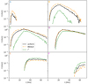 |
Fig. 6. Intensity profiles for the three radial injection functions of Fig. 1 at each of the six observers in Table 2 with scattering conditions described by λ = 0.1 au. Injection is uniform in θ, ϕ. |
For observer D all three injections are very similar, with the r2 injection having slightly lower intensities during the rise phase. For more eastern events (observers E and F), the r2 injection shows the largest intensities due to these observers connecting to the shock at larger radial distances where larger numbers of particles are injected. It is clear from these plots that geometric effects such as the time of observer-shock connection or disconnection as well as the corotation of particle-filled flux tubes towards or away from the observer have a much more significant effect on the intensity profile than the radial injection function.
The peak intensity, Ipeak, is plotted in Fig. 7 vs. Δϕ (defined in Eq. (16)) for the three shock-like radial injection functions. Each set of points is fit with a Gaussian of the form I = I0exp(−(ϕ − ϕ0)2/2σ2). Table 3 shows the values of ϕ0, σ, and I0 for the fits shown in Fig. 7. The largest intensities are obtained for the Weibull R(r), which injects most particles close to the Sun, while the r2 injection function results in much lower Ipeak values. The standard deviations of the uniform and Weibull function injections are similar, while the r2 injection has a larger standard deviation. The peak intensities at observers B and C are lower for the r2 injection compared to the other injection functions as the number of particles injected close to the Sun is smaller. However, at observers D, E, and F, larger intensities are seen because the shock continues to inject particles late into the event. Figure 7 also shows that the broadness of the Gaussian is more closely related to the number of particles injected per unit area of the shock front, Q(r), rather than R(r). The centre of the Gaussian, ϕ0, is shifted towards more negative values as one goes from Weibull to uniform to r2R(r).
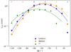 |
Fig. 7. Peak intensity vs. Δϕ for the three radial injection functions. |
5.4. Dependence on varying injection efficiency across the shock
In Fig. 8 intensity profiles are shown when considering injection efficiencies across the shock in longitude and colatitude (Φ(ϕ), Θ(θ)) that are a) uniform (solid black line) and b) Gaussian (red dashed line) with σ = 17.5° centred on the shock nose (see Fig. 2). It is apparent that changing the injection efficiency across the shock produces only small changes in the intensity profiles. For the Gaussian injection function at times when the observer’s cobpoint lies near the shock nose (observers B and C), there is a faster increase compared to the uniform case during the rise phase and a larger peak intensity. Observers A and F, which experience connection to the flanks of the shock, have smaller intensities compared to the uniform injection case, but the differences are small. Changing the injection profiles across the shock does not have a big influence on the overall features of the intensity profiles.
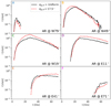 |
Fig. 8. Intensity profiles for observers A–F at 1 au considering uniform and Gaussian longitudinal and latitudinal injection functions, with λ = 0.1 au. Injection is uniform in r. |
In Fig. 9 we plotted the peak intensity vs. Δϕ for uniform and Gaussian injection efficiency across the shock. Both sets of points are fitted with a Gaussian and the corresponding fit parameters are given in Table 3. As expected, having a Gaussian injection reduces the standard deviation of the fit due to the more spatially confined injected population.
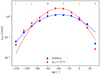 |
Fig. 9. Peak intensity vs. Δϕ for shocks with uniform (blue circles) or Gaussian (red diamonds, σ = 17.5°) longitudinal and latitudinal injection efficiency. The shocks have an angular width of 70°. Both sets of points are fitted with Gaussians (dashed lines). |
5.5. Role of shock width
We have considered shocks of different angular widths. In Fig. 10 we compare intensity profiles at the six observers for shocks with wsh, ϕ = wsh, θ = 70° (black line) and 120° (orange dashed line).
 |
Fig. 10. Intensity profiles at the six observers considering a shock 70° (solid black line) and 120° (orange dashed line) in both longitude and latitude. |
One effect of a wider shock is that an observer can remain magnetically connected to the shock front for a longer period of time. This factor changes the rise times for western events because the peak position in the intensity profiles is determined by the loss of connection to the shock front. This can be seen in Fig. 10 for observers A and B where the rise times are extended and peak intensities occur later. Observations at C are similar in the two cases as the peak intensity occurs as the shock passes directly over the observer. We note that the exact values of the intensities are not directly comparable in these simulations as the same number of particles are injected over a larger volume for the wider shock (i.e., different Q(r)). For a wider shock at observers that see the event as being eastern, onsets take place earlier as the observer-shock connection is established more quickly when the shock is closer to the Sun, as can be seen in Fig. 10 for observers D, E, and F.
5.6. Observers at 0.3 au
We used our simulations to obtain observables close to the Sun and compare them with 1 au observables. This is important now that Parker Solar Probe and Solar Orbiter are obtaining in situ data in the inner heliosphere.
Having fixed an observer at 1 au, in Fig. 11, intensity and anisotropy profiles are plotted for two 0.3 au observers: the first radially in line with the 1 au observer (left column) and the second on the same IMF line (right column). Profiles at the 1 au observer are indicated by the dash-dotted lines for comparison. A uniform R(r) was used.
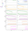 |
Fig. 11. Schematic of observer geometry (left), with observer 1 located at 0.3 au, radially aligned with the 1 au observers, and with 2 located at 0.3 au along the same IMF line as the 1 au observer. Intensity and anisotropy profiles (right) for observers 1 and 2 (solid curves) and 1.0 au observer (dash-dotted curves). |
Compared to the 1 au profiles, the 0.3 au profiles are characterised by the following: faster rise times, due to faster shock passage times at 0.3 au, and larger anisotropies (1 au anisotropies not shown) as there is reduced isotropisation due to fewer pitch-angle scattering events.
Generally the profiles at 0.3 and 1.0 au appear more similar for the case of observers on the same IMF line (right column), than for the radially in-line observers (left column). In the former case, both observers establish magnetic connection to the shock at similar times, with some difference due to propagation times. For the case of radially in-line 0.3 and 1.0 observers (left column), there are stronger differences between the profiles compared to the previous case. For observers D, E, and F, the onset at 0.3 au is more than 10 h earlier than at 1 au. This is due to the fact that the radially aligned 0.3 au observers have footpoints located eastwards of the 1 au observer, meaning that for eastern events they will connect to the shock earlier. The decay time constants of the event appear significantly different at 0.3 and 1.0 au.
Considering peak intensities for the same IMF line case, for observers B–F the peak intensity at 1.0 au is larger than at 0.3 au. This is because particle injection before shock arrival is more extended for the 1 au observer. After shock passage, although particles can propagate sunwards to the observer, this becomes difficult due to magnetic mirroring (Hutchinson et al. 2022). For the observer A panel, the 0.3 au intensity is larger because both 0.3 and 1 au observers lose connection early in the event and scattering and propagation delay result in lower peak intensity at 1 au. The intensity profiles observed at 0.3 au have a weak dependence on λ (not shown). Eastern events show much slower decay phases compared to western events, similar to the 1.0 au observers.
We note that when close to the Sun, Parker Solar Probe and Solar Orbiter are moving in longitude at a high speed so that the intensity profiles shown in Fig. 11, where the 0.3 au observer is stationary, do not correspond exactly to those measured by these spacecraft. In some phases of the mission, Solar Orbiter will be corotating with the Sun.
We have analysed the intensity profiles (not shown) at 0.3 au for the three radial injection profiles considered earlier (see Fig. 1) and they display a behaviour similar to that in Fig. 6, that is to say not a strong dependence on R(r).
6. Discussion and conclusions
In this paper we have presented the first 3D test particle simulations of SEPs with a temporally extended shock-like particle injection. Previously, in our modelling we had only considered an instantaneous injection near the Sun. By deriving the intensity and anisotropy profiles for observers at 0.3 and 1.0 au, we have reached the following main conclusions:
-
The main difference between an instantaneous and time-extended injection is that, in the former case, the spatial extent of the accelerated particle population is smaller (Fig. 5). For initially well-connected observers (A–C), the duration of the SEP event is not significantly shorter for an instantaneous injection compared to an extended one.
-
The radial profile of injection (radial injection function, R(r), Fig. 1) plays a surprisingly small role in determining the intensity profiles at 1 au (Fig. 6). However, R(r) has a strong effect on the heliolongitudinal distribution of peak intensity (Fig. 7) with injections that continue over larger radial distances leading to more negative ϕ0 values and larger standard deviations.
-
Varying the injection efficiency across the shock (longitudinal and latitudinal injection functions, Φ(ϕ), Θ(θ), Fig. 2) also plays a minor role in shaping intensity profiles (Fig. 8).
-
In most cases simulations show large persistent anisotropies prior to shock passage and they decay sharply at shock arrival, becoming very close to zero following shock passage (Fig. 4, observers A–D). For observers that see the event far in the east, the first arriving particles are propagating sunwards once connection to the shock is established.
-
Larger shock widths lead to longer duration SEP events because the observers remain connected to the shock for a longer time.
-
Intensity profiles at 0.3 au are similar to those at 1.0 au for two observers on the same IMF line, but they show faster rise times and larger anisotropies.
Our simulations show that the link between the duration of injection and the duration of the SEP event is very weak, unlike what is commonly assumed. Also from our simulations it is not clear that differences in the acceleration efficiencies at the flanks of the shock would leave a signature in the observed intensity profiles, as is often postulated (e.g., Tylka & Lee 2006). Spatial and geometric factors such as the establishment and loss of the observer-shock connection and the corotation of the particle-filled flux tubes towards and away from the observer are the dominant factors in determining the shapes and properties of SEP intensity profiles. The role of corotation is fully illustrated in a companion paper (Hutchinson et al. 2023). Intensity profiles show little dependence on the mean free path, λ. In particular the decay phase constant is weakly dependent on λ, unlike what is derived from 1D focussed transport models (e.g., Bieber et al. 1994).
A number of studies of SEP observations have derived plots of peak intensity vs. the separation Δϕ between the source AR and observer footpoint (e.g., Wiedenbeck et al. 2013; Lario et al. 2013; Cohen et al. 2014; Richardson et al. 2014). Our work shows that these plots are sensitive to the radial injection profile and longitudinal and latitudinal injection efficiency. When a lot of acceleration takes place in interplanetary space, the centre ϕ0 of the Gaussian fit to the Ipeak vs. Δϕ plot is shifted towards more negative values compared to cases where most of the acceleration takes place close to the Sun. For the shock width considered in our study, which is 70°, standard deviations between 26° and 38° are found.
In this paper we have presented results for a monoenergetic proton population injected with energy of 5 MeV, which is a representative SEP energy. The difficulty in considering multiple energies lies in the need to specify how the radial injection function, R(r), varies with energy. In addition, because of particle deceleration, the final particle energy in our simulations is smaller than 5 MeV for some particles. In constructing the intensity profiles in this paper, we have chosen to include all particles > 1 MeV. In actual SEP events, a spectrum of energies would actually be injected and particles of higher energy would decelerate into the 5 MeV range. Limiting the range of energies in the plot to a smaller energy range near 5 MeV produces some modifications in the profiles, but it does not change the qualitative trends we have found. For particle energies much higher than 5 MeV, injections are thought to take place only close to the Sun, limiting the range of longitudes of the shock source. For these higher energy particles, drift effects may be important in determining the range of accessible longitudes during an SEP event (Dalla et al. 2013).
Our model did not include magnetic field line meandering (Laitinen et al. 2016), which would lead to significant motion of the particles perpendicular to the mean magnetic field. This effect could potentially explain some features of our modelled intensity profiles that do not agree with SEP observations: for eastern events our simulations do not show the slow rise phase found in observations (e.g., Cane et al. 1988; Kahler 2016), displaying instead very delayed onsets and relatively fast rises. The inclusion of perpendicular transport may produce the observed long rise times as long as the process is slow. It might be possible to determine a limit to the strength of perpendicular transport by modelling the slow rise times during eastern events. Considering the plots of Ipeak vs. Δϕ (Figs. 7 and 9), perpendicular diffusion would increase the peak intensity at the less well-connected observers, resulting in a larger standard deviation of the Gaussian fits. It is expected that with the inclusion of perpendicular diffusion, intensity profiles at widely separated locations will become more similar to each other. We hope to include the effects of turbulence-induced perpendicular transport in future work.
The anisotropy characteristics shown in Fig. 4, namely the large persistent anisotropies and the sunward anisotropies for far eastern events, are not routinely detected in SEP events to our knowledge. It is possible that this may be due to perpendicular transport effects.
While our model of shock-like injection has allowed us to derive the qualitative patterns described above, it contains several simplifications that will need to be improved upon in future work. Our simulation neither models shock acceleration nor the interaction of energetic particles with the shock. We have not considered how the shock decelerates with time: this would affect the extent of the event since IMF field lines towards the west would only be reached at later times.
The simulations in the present study do not include the heliospheric current sheet (HCS), which has been shown to have significant effects for SEP propagation when the source region is located close to it (Battarbee et al. 2017, 2018; Waterfall et al. 2022). Individual events, depending on the magnetic configuration, may be significantly influenced by the HCS due to strong HCS drift motions, especially for high energy SEPs (Waterfall et al. 2022).
Other factors which may influence intensity profiles are the complex local magnetic field and solar wind structures, not included in our model at present. Any perturbations to the Parker spiral will affect the times of observer-shock connection and so will affect observable parameters such as onset times and peak times. Some structures such as corotating interaction regions (Wijsen et al. 2019) or magnetic clouds (Kallenrode 2002) may significantly affect SEP transport affecting intensity profiles.
Acknowledgments
A. Hutchinson, S. Dalla and T. Laitinen acknowledge support from the UK Science and Technology Facilities Council (STFC), through a Doctoral Training grant – ST/T506011/1 and grants ST/R000425/1 and ST/V000934/1. C.O.G. Waterfall and S. Dalla acknowledge support from NERC grant NE/V002864/1. This work was performed using resources provided by the Cambridge Service for Data Driven Discovery (CSD3) operated by the University of Cambridge Research Computing Service (www.csd3.cam.ac.uk), provided by Dell EMC and Intel using Tier-2 funding from the Engineering and Physical Sciences Research Council (capital grant EP/P020259/1), and DiRAC funding from the Science and Technology Facilities Council (www.dirac.ac.uk).
References
- Baring, M. G. 1997, in Very High Energy Phenomena in the Universe; Moriond Workshop, eds. Y. Giraud-Heraud, & J. Tran Thanh van, 97 [Google Scholar]
- Battarbee, M., Dalla, S., & Marsh, M. S. 2017, ApJ, 836, 138 [NASA ADS] [CrossRef] [Google Scholar]
- Battarbee, M., Dalla, S., & Marsh, M. S. 2018, ApJ, 854, 23 [NASA ADS] [CrossRef] [Google Scholar]
- Bieber, J. W., Matthaeus, W. H., Smith, C. W., et al. 1994, ApJ, 420, 294 [Google Scholar]
- Cane, H. V., Reames, D. V., & von Rosenvinge, T. T. 1988, J. Geophys. Res. Space Phys., 93, 9555 [NASA ADS] [CrossRef] [Google Scholar]
- Cohen, C. M. S., Mason, G. M., Mewaldt, R. A., & Wiedenbeck, M. E. 2014, ApJ, 793, 35 [NASA ADS] [CrossRef] [Google Scholar]
- Dalla, S., & Browning, P. K. 2005, A&A, 436, 1103 [NASA ADS] [CrossRef] [EDP Sciences] [Google Scholar]
- Dalla, S., Marsh, M., Kelly, J., & Laitinen, T. 2013, J. Geophys. Res. Space Phys., 118, 5979 [NASA ADS] [CrossRef] [Google Scholar]
- Dalla, S., de Nolfo, G. A., Bruno, A., et al. 2020, A&A, 639, A105 [NASA ADS] [CrossRef] [EDP Sciences] [Google Scholar]
- Desai, M., & Giacalone, J. 2016, Liv. Rev. Sol. Phys., 13 [Google Scholar]
- Gopalswamy, N., et al. 2013, Adv. Space Res., 51, 1981 [NASA ADS] [CrossRef] [Google Scholar]
- He, H.-Q., Qin, G., & Zhang, M. 2011, ApJ, 734, 74 [NASA ADS] [CrossRef] [Google Scholar]
- Heras, A. M., Sanahuja, B., Sanderson, T. R., Marsden, R. G., & Wenzel, K. P. 1994, J. Geophys. Res. Space Phys., 99, 43 [NASA ADS] [CrossRef] [Google Scholar]
- Hutchinson, A., Dalla, S., Laitinen, T., et al. 2022, A&A, 658, A23 [NASA ADS] [CrossRef] [EDP Sciences] [Google Scholar]
- Hutchinson, A., Dalla, S., Laitinen, T., & Waterfall, C. O. G. 2023, A&A, 670, L24 [NASA ADS] [CrossRef] [EDP Sciences] [Google Scholar]
- Kahler, S. W. 2016, ApJ, 819, 105 [NASA ADS] [CrossRef] [Google Scholar]
- Kahler, S. W., & Ling, A. G. 2018, Sol. Phys., 293, 30 [NASA ADS] [CrossRef] [Google Scholar]
- Kallenrode, M.-B. 2001, J. Geophys. Res. Space Phys., 106, 24989 [NASA ADS] [CrossRef] [Google Scholar]
- Kallenrode, M.-B. 2002, J. Atmos. Solar-Terrest. Phys., 64, 1973 [NASA ADS] [CrossRef] [Google Scholar]
- Kallenrode, M.-B., & Wibberenz, G. 1997, J. Geophys. Res. Space Phys., 102, 22311 [NASA ADS] [CrossRef] [Google Scholar]
- Klein, K. L., Tziotziou, K., Zucca, P., et al. 2018, in Solar Particle Radiation Storms Forecasting and Analysis, eds. O. E. Malandraki, & N. B. Crosby, 444, 133 [NASA ADS] [CrossRef] [Google Scholar]
- Laitinen, T., Kopp, A., Effenberger, F., Dalla, S., & Marsh, M. S. 2016, A&A, 591, A18 [NASA ADS] [CrossRef] [EDP Sciences] [Google Scholar]
- Lario, D., Sanahuja, B., & Heras, A. M. 1998, ApJ, 509, 415 [NASA ADS] [CrossRef] [Google Scholar]
- Lario, D., Aran, A., Gómez-Herrero, R., et al. 2013, ApJ, 767, 41 [CrossRef] [Google Scholar]
- Marsh, M. S., Dalla, S., Kelly, J., & Laitinen, T. 2013, ApJ, 774, 4 [NASA ADS] [CrossRef] [Google Scholar]
- Marsh, M. S., Dalla, S., Dierckxsens, M., Laitinen, T., & Crosby, N. B. 2015, Space Weather, 13, 386 [CrossRef] [Google Scholar]
- Qin, G., Wang, Y., Zhang, M., & Dalla, S. 2013, ApJ, 766, 74 [NASA ADS] [CrossRef] [Google Scholar]
- Reames, D. V., Kahler, S. W., & Ng, C. K. 1997, ApJ, 491, 414 [NASA ADS] [CrossRef] [Google Scholar]
- Richardson, I. G., von Rosenvinge, T. T., Cane, H. V., et al. 2014, Sol. Phys., 289, 48 [NASA ADS] [Google Scholar]
- Tylka, A. J., & Lee, M. A. 2006, ApJ, 646, 1319 [NASA ADS] [CrossRef] [Google Scholar]
- Wang, Y., Qin, G., & Zhang, M. 2012, ApJ, 752, 37 [CrossRef] [Google Scholar]
- Waterfall, C. O. G., Dalla, S., Laitinen, T., Hutchinson, A., & Marsh, M. 2022, ApJ, 934, 82 [NASA ADS] [CrossRef] [Google Scholar]
- Wiedenbeck, M. E., Mason, G. M., Cohen, C. M. S., et al. 2013, ApJ, 762, 54 [NASA ADS] [CrossRef] [Google Scholar]
- Wijsen, N., Aran, A., Pomoell, J., & Poedts, S. 2019, A&A, 622, A28 [NASA ADS] [CrossRef] [EDP Sciences] [Google Scholar]
- Zank, G. P., Li, G., Florinski, V., et al. 2006, J. Geophys. Res. Space Phys., 111, A06108 [NASA ADS] [CrossRef] [Google Scholar]
All Tables
All Figures
|
Fig. 1. Radial injection function, R(r) vs. r (top), and the number of particles injected per unit area of the shock, Q(r) vs. r (bottom). |
| In the text | |
|
Fig. 2. Longitudinal injection function, Φ(ϕ), for the shock-like injection. |
| In the text | |
|
Fig. 3. Diagrams showing the shock position and observer geometry at t = 0 (top left), 16 (top right), 32 (bottom left), and 48 (bottom right) hours projected onto the solar equatorial plane. Here x and y are heliocentric Cartesian coordinates in the heliographic equatorial plane. The shock’s projection onto the plane is displayed here as the orange shaded segments. Observers A-F are denoted by the coloured circles, and their exact positions are displayed in Table 2. The red radial dashed lines delimit the bounds of the shock, and the solid red curved lines show the IMF lines that are currently connected to the flanks of the shock front. The solid green curved lines show the bounds of the shock-like injection at the initial time (or equally an instantaneous injection at the Sun of the same angular width). The dashed green line shows the original position of the left most solid green line at the initial time. The grey IMF lines represent the range of IMF lines that have had particles injected onto them (the particle-filled flux tubes). |
| In the text | |
|
Fig. 4. Intensity profiles of a monoenergetic population of 5 MeV protons for observers A–F at 1.0 au for a range of scattering conditions from λ = 0.1 au to λ = 1.0 au, for uniform injection in r, θ, and ϕ. The green dashed line indicates the time at which the shock reaches the observer radial distance, and the vertical dotted line shows the time when the observer establishes connection to the shock, for observers not connected at the initial time. |
| In the text | |
|
Fig. 5. Intensity profiles for observers A–F considering an instantaneous injection (blue dashed lines) and an extended uniform injection (solid black lines) with respect to r, θ, and ϕ. The injection region is 70° in both cases. The simulations use λ = 0.1 au. |
| In the text | |
|
Fig. 6. Intensity profiles for the three radial injection functions of Fig. 1 at each of the six observers in Table 2 with scattering conditions described by λ = 0.1 au. Injection is uniform in θ, ϕ. |
| In the text | |
|
Fig. 7. Peak intensity vs. Δϕ for the three radial injection functions. |
| In the text | |
|
Fig. 8. Intensity profiles for observers A–F at 1 au considering uniform and Gaussian longitudinal and latitudinal injection functions, with λ = 0.1 au. Injection is uniform in r. |
| In the text | |
|
Fig. 9. Peak intensity vs. Δϕ for shocks with uniform (blue circles) or Gaussian (red diamonds, σ = 17.5°) longitudinal and latitudinal injection efficiency. The shocks have an angular width of 70°. Both sets of points are fitted with Gaussians (dashed lines). |
| In the text | |
|
Fig. 10. Intensity profiles at the six observers considering a shock 70° (solid black line) and 120° (orange dashed line) in both longitude and latitude. |
| In the text | |
|
Fig. 11. Schematic of observer geometry (left), with observer 1 located at 0.3 au, radially aligned with the 1 au observers, and with 2 located at 0.3 au along the same IMF line as the 1 au observer. Intensity and anisotropy profiles (right) for observers 1 and 2 (solid curves) and 1.0 au observer (dash-dotted curves). |
| In the text | |
Current usage metrics show cumulative count of Article Views (full-text article views including HTML views, PDF and ePub downloads, according to the available data) and Abstracts Views on Vision4Press platform.
Data correspond to usage on the plateform after 2015. The current usage metrics is available 48-96 hours after online publication and is updated daily on week days.
Initial download of the metrics may take a while.