| Issue |
A&A
Volume 674, June 2023
Gaia Data Release 3
|
|
|---|---|---|
| Article Number | A9 | |
| Number of page(s) | 14 | |
| Section | Catalogs and data | |
| DOI | https://doi.org/10.1051/0004-6361/202243969 | |
| Published online | 16 June 2023 | |
Gaia Data Release 3
Astrometric binary star processing
1
Université de Strasbourg, CNRS, Observatoire Astronomique de Strasbourg, UMR 7550, 11 rue de l’Université, 67000 Strasbourg, France
e-mail: This email address is being protected from spambots. You need JavaScript enabled to view it.
2
FNRS, Institut d’Astronomie et d’Astrophysique, Université Libre de Bruxelles, Boulevard du Triomphe, 1050 Bruxelles, Belgium
3
GEPI, Observatoire de Paris, Université PSL, CNRS, 5 Place Jules Janssen, 92190 Meudon, France
4
Université Côte d’Azur, Observatoire de la Côte d’Azur, CNRS, Laboratoire Lagrange, Bd de l’Observatoire, CS 34229, 06304 Nice Cedex 4, France
5
IMCCE, Observatoire de Paris, Université PSL, CNRS, Sorbonne Université, Univ. Lille, 77 Av. Denfert-Rochereau, 75014 Paris, France
6
Telespazio UK S.L. for ESA/ESAC, Camino bajo del Castillo, s/n, Urbanizacion Villafranca del Castillo, Villanueva de la Cañada, 28692 Madrid, Spain
Received:
6
May
2022
Accepted:
25
June
2022
Abstract
Context. The Gaia Early Data Release 3 contained the positions, parallaxes, and proper motions of 1.5 billion sources, some of which did not show a good fit to the ‘single star’ model. Binarity is one of the causes of this.
Aims. Four million of these stars were selected and various models were tested to detect binary stars and to derive their parameters.
Methods. We used a preliminary treatment to discard the partially resolved double stars and to correct the transits for perspective acceleration. We then investigated whether the measurements show a good fit to an acceleration model with or without jerk. We tried the orbital model when the fit of any acceleration model was beyond our acceptance criteria. We also tried a Variability-Induced Mover (VIM) model when the star was photometrically variable. A final selection was made in order to keep only solutions that probably correspond to the real nature of the stars.
Results. Following our analysis, 338 215 acceleration solutions, about 165 500 orbital solutions, and 869 VIM solutions were retained. In addition, formulae for calculating the uncertainties of the Campbell orbital elements from orbital solutions expressed in Thiele-Innes elements are given in an appendix.
Key words: binaries: general / catalogs / astrometry / methods: data analysis
Deceased on 14 November 2021.
© The Authors 2023
 Open Access article, published by EDP Sciences, under the terms of the Creative Commons Attribution License (https://creativecommons.org/licenses/by/4.0), which permits unrestricted use, distribution, and reproduction in any medium, provided the original work is properly cited.
This article is published in open access under the Subscribe to Open model. This email address is being protected from spambots. You need JavaScript enabled to view it. to support open access publication.
1. Introduction
Since the start of the Gaia satellite observations in summer 2014, several data releases have been made available to the scientific community. The astrometric parameters of more than one billion stars have been determined three times with ever increasing precision, but these data still described the stars as single. The third Data Release (DR3) and the Early third Data Release (EDR3) are the first to have a significant number of observations covering a sufficiently long time span (about 33 months) to make it worthwhile to use Gaia observations to search for binary stars.
The extension of the exploitation of Gaia observations to binary stars reveals two difficulties in addition to the application of the single star model. As with its predecessor HIPPARCOS, the double-star candidates are covered by different numerical models, with uncertainty remaining as to whether any of them really corresponds to a given star. Therefore, we have to solve the problem of choosing the model that best applies to a given star, as well as the final acceptance of the solution. Before that, we have to filter the input data to retain only those stars for which a suitable solution can be obtained.
2. Treatment overview
2.1. Selection of stars to be processed
The astrometric processing of the Gaia Early Data Release 3 (EDR3, Gaia Collaboration 2021) left some 36.5 million stars that were considered to be possibly double. These stars were all brighter than G = 19, had a renormalised unit weight error (RUWE; see Lindegren et al. 2021) of greater than 1.4, and were observed over at least 12 visibility periods. These objects included many pairs of stars that were resolved whenever the orientation of the scan direction made this possible, and were seen as a single photocentre otherwise. These so-called ‘partially resolved double stars’ are likely to appear as unresolved binary stars of extremely rapid orbital motion, and should be discarded wherever possible. It is planned to apply a specific treatment to them in future data releases, but for the moment we can only eliminate them when possible. For this purpose, two quantities published in Gaia EDR3 and coming from the astrometric binary-detection processing (Lindegren et al. 2021) were used to establish two additional criteria: the percentage of CCD observations where image parameter determination (IPD) detected more than one peak, called ipd_frac_multi_peak, must be less than or equal to 2, and ipd_gof_harmonic_amplitude, which is the amplitude of the natural logarithm of the goodness-of-fit obtained in the IPD versus the scan position angle, must be less than 0.1. As a result, the number of targets to be treated was reduced to 10.9 million. In order to further reduce the number of partially resolved double stars, a final selection was based on photometric properties. As the pixels of the astrometric field are much smaller than those of the blue and red photometers (BP and RP) windows, a component of a close binary at the resolution limit appears less bright in G magnitude (from the astrometric field) than one would expect from its magnitude in the BP and RP fields. The corrected BP and RP flux excess factor C* and its uncertainty σC* as defined in Riello et al. (2021, Eqs. (6) and (18)) were taken into account. The drastic condition |C*|< 1.645 σC*, corresponding to a 90% confidence interval, was applied and a selection of 4 115 743 stars was finally obtained.
2.2. Overall organisation
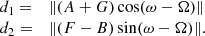
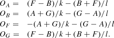
The organisation of the astrometric binary star processing, as it was finally realised, is summarised in Fig. 1. The input data consist of the 4 115 743 selected stars, for which the following information is used: the along-scan (AL) coordinates of each transit of the astrometric field of view, the partial derivatives of the single star astrometric model, the G magnitudes of the transits, and the parameters of a preliminary single star solution, that is, the coordinate offsets, the parallax, and the proper motion. The production of the astrometric data is described in Lindegren et al. (2021), while the magnitude reduction is explained in Riello et al. (2021). The data are complemented by radial velocities, when available (Seabroke et al., in prep.).
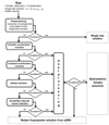 |
Fig. 1. Overall organisation of the astrometric treatment of binary stars, as was eventually applied to the DR3. The cascade on the left side of the figure is the ‘main processing’ referred to hereafter. |
The calculation of the astrometric solutions is done in the so-called main processing, as explained hereafter. The data discussed above are ingested by the preprocessing, which prepares them for the calculation of different types of solutions. The solutions are calculated one after the other, starting with a new calculation of the single star solution, followed by the acceleration solutions, the orbital solution, and, finally, the variability-induced mover (VIM) solutions if the star is photometrically variable. As soon as a solution is considered acceptable, the processing cascade is interrupted and the star goes to post-processing. The post-processing essentially consists of re-filtering the solutions, applying more stringent criteria than those used after the solutions were calculated. When a solution is discarded by post-processing, it is replaced by the EDR3 single-star solution.
In practice, the software for managing the cascade of calculation and acceptance of solutions is much more sophisticated than the scheme shown in Fig. 1. Indeed, the solution that entered the post-processing was sometimes a so-called ‘alternative’ solution (not to be confused with the ‘OrbitalAlternative’ solutions in Holl et al. 2023): a solution that met poor acceptance criteria, and which was retained because it was the solution that best matched the observations at the end of the cascade. More information on this aspect of the process is given at the end of Sect. 2.3.2, but we can already highlight two things: First, that we did not systematically try all the models to retain the one that was the most suitable; this was motivated mainly by the objective to save computational time, but also by the fear of accepting complex solutions for objects that could fall under a simpler model (e.g., giving an acceleration solution for an orbital binary is a less serious error than giving a false orbital solution for a binary that should only have an acceleration solution). Despite its apparent mathematical simplicity, the VIMF model has been placed at the end because it combines data of two kinds (astrometric and photometric), which undermines the reliability of the solutions. Secondly, post-processing consists only of rejecting solutions, without trying to replace them with more complex or alternative solutions. Ideally, the filters applied in post-processing should be included in the main processing, but this was not possible in the time available.
2.3. Criteria for the acceptance of solutions
We define hereafter two quality criteria, the goodness of fit and the significance, which can be used to distinguish acceptable solutions from those that are irrelevant or at least potentially wrong. In order to decide whether or not a solution is really plausible, we also consider astrophysical criteria and other constraints, which allows us to identify some solutions as not very plausible. These bad solutions allow us to delimit a quality domain where they are absent or rare, and whose solutions will be kept.
2.3.1. The goodness of fit
The goodness of fit indicates whether or not the model provides predictions that are compatible with the actual measurements. As in the preparation of the HIPPARCOS catalogue (ESA 1997, Vol. 1, Sect. 2.1), we use the F2 estimator, which is given by the formula:
![Mathematical equation: $$ \begin{aligned} F_2 = \sqrt{\frac{9 \nu }{2}}\left[ \left( \frac{\chi ^2}{\nu }\right)^{1/3} + \frac{2}{9 \nu } - 1 \right] , \end{aligned} $$](/articles/aa/full_html/2023/06/aa43969-22/aa43969-22-eq1.gif) (1)
(1)
where ν is the number of degrees of freedom, and χ2 is the sum of the squared normalised residuals. For a solution derived through an adequate model, F2 is expected to obey the normal distribution 𝒩(0, 1). This property is attributed to linear models (Stuart & Ord 1994), but we verified using simulations that it also applies to the orbital model presented hereafter, when the semi-major axis of the orbit is significantly larger than its uncertainty. A large F2 means that the model is inadequate, or that the uncertainties used to derive the χ2 are underestimated. In practice, we know that this last possibility widely applies to the astrometric transits used in DR3. Therefore, only very large values of F2 indicate that the model cannot be accepted. Nevertheless, assuming that the model is adequate, the uncertainties may be revised in order to obtain a zero F2. The simplest correction method, as it keeps the relative weights of the transits and therefore the solution of the model, consists in multiplying the uncertainties of the observations by the coefficient:
 (2)
(2)
It is worth noting that the correction by the coefficient c also applies to the uncertainties of the model parameters. In addition to the correction of uncertainties, F2 was also taken into account for the selection of solutions. In the main processing, solutions of F2 > 1000, if any, were rejected, but a stricter condition was applied in the post-processing: whatever the model, purely astrometric solutions with uncorrected F2 > 25 were considered as questionable, and were finally not retained.
Although similar in principle, this approach is slightly different from that followed in the treatment of single star solutions for EDR3 (Lindegren et al. 2021): Eq. (2) shows that the coefficient c is equal to UWE × [1−(2/9ν)]−3/2, which is approximately equal to UWE. On the other hand, we do not apply a renormalisation, but this does not matter because we only consider stars brighter than G = 19.
2.3.2. The significance
The significance is a dimensionless quantity that was already introduced in the HIPPARCOS catalogue (ESA 1997, Vol. 1, Sect. 2.3.3) in order to decide whether the use of a model including additional parameters is really justified. When the additional parameters are the coordinates of a two-dimensional vector, as is the case for the acceleration models in Sect. 4, the significance, s, is defined as the module of this vector divided by its uncertainty. Therefore, s is calculated with the equation:
 (3)
(3)
where p1 and p2 are the coordinates of the additional vector characterising the model (e.g., the acceleration), σ1 and σ2 are the uncertainties of p1 and p2, respectively, corrected by the coefficient c derived with Eq. (2), and ρ12 is the correlation coefficient between p1 and p2. The values of σ1, σ2, and ρ12 are all taken from the variance-covariance matrix.
When the solutions were calculated, a preliminary selection was made through basic filtering: the solutions of s > 12 and F2 < 25 were considered good enough to be retained, without trying other models. Otherwise, the solutions with s > 5 and F2 < 1000 were considered as ‘alternative’ solutions (see Sect. 2.2), and the smaller F2 alternative was provisionally accepted at the end of the cascade. The limit of 5 was adopted empirically on the basis of initial tests of the data. Thresholds of 5 and 12, which amount to as many σs, seem exceptionally high and are much higher than the thresholds of 3 and 4 that were adopted on the basis of simulations for alternative solutions and for direct acceptance, respectively. This is because, in reality, the uncertainties on the transits of a star are certainly not all overestimated by the same coefficient; correcting the uncertainties by a single coefficient is only a ‘stopgap’ measure, as it is not possible to separate transits with a correct original uncertainty from those with a very underestimated uncertainty.
The set of solutions selected as above was then subjected to a more severe filtering in order to keep only the most credible solutions, as explained below for each model. The final selection criteria, resulting from main processing followed by post-processing, are presented in Table 1. For the acceleration models and for the VIMF model, these are more severe than the direct acceptance criteria, and they lead to the rejection of alternative solutions. However, all alternative solutions contribute to the statistical properties of the main processing solutions, which are presented hereafter, and are the basis for the choice of the final criteria.
Properties of the different models and final conditions for the selection of solutions.
3. Preprocessing
3.1. Rejection of outliers
Each transit of a star through the Gaia astrometric instrument comes down to the measurement of two coordinates, which give its position relative to a reference point assigned to the star (see Lindegren et al. 2021). Of these, only the coordinate along the scan axis, hereafter referred to as the AL abscissa, w, is taken into account, as it is considerably more accurate than the other. The AL abscissae were measured along the nine CCD transits that constitute each field-of-view (FoV) transit. As the duration of the FoV transit is only a few seconds, while we are looking for binary stars with periods of at least several days, the nine CCD transits amount to nine measurements of the same quantity. Outliers were therefore detected by intercomparison between the CCD transits. In practice, each AL abscissa was compared to the median of the nine values, and the transit CCD was rejected when the difference exceeded five times the uncertainty on the abscissa.
This rejection process was not the only one that was applied, and subsequently transits were rejected after the calculation of some astrometric solutions. The largest residual transit was rejected when it exceeded five times the uncertainty, and the solution was recalculated; however, this operation was subject to three restrictions: (1) it was only done for linear models, that is, the single star model and the two acceleration models; (2) the χ2 of the solution should exceed the number of transits used multiplied by 1.41; and (3) the proportion of rejected transits was limited to 5%.
3.2. Correction of the perspective acceleration
The distance from the Sun and the apparent position of a nearby star vary during the time-span of the Gaia mission, inducing slight changes in astrometric parameters, which are usually assumed to be constant. These so-called ‘perspective effects’ were taken into account in the calculation of the astrometric parameters of a few single stars in the HIPPARCOS catalogue (ESA 1997). Dravins et al. (1999) and Lindegren & Dravins (2003) showed that these effects are so closely related to radial velocity that they could be used to measure it. For Gaia, Halbwachs (2009) showed that perspective effects do not significantly affect the astrometric orbits of binary stars; however, they do result in a ‘perspective acceleration’ of stars that could be mistaken for an acceleration due to orbital motion.
The perspective acceleration is based on the radial proper motion, μr, which is defined as the radial velocity, vr, divided by distance. In practice, μr, expressed in yr−1, is related to vr and parallax, ϖ, by the following relationship:
 (4)
(4)
where vr is in km s−1, ϖ is in mas, yeardays is the duration of the year in days, and aum is the length of the astronomical unit (au) in meters. Perspective acceleration changes the AL abscissa of a star, w, by adding the following quantity:
 (5)
(5)
where t is the epoch in years, and T is an epoch close to the middle of the DR3 mission (in practice, T = 2016.0). The partial derivatives of the abscissa with respect to the parallax and to the proper motion coordinates are those of the five-parameter single star model. If μr is unknown, then the abscissae are related to the parameters by a system of non-linear equations. Fortunately, the radial velocities of the bright stars are measured by Gaia, and a calculation based on the single star model, ignoring the perspective acceleration, already gives a good approximation of the parallax and of the proper motion. Therefore, μr may be determined from Eq. (4).
There are therefore two possible ways to take into account the perspective acceleration: either multiply the partial derivatives by μr(t − T), as they are in Eq. (5), or correct the abscissae by subtracting the perspective acceleration contribution, Δw. Because of its simplicity, we followed the latter method: Δw was calculated from Eq. (5) using preliminary values of ϖ, μα*, and μδ, and was subtracted from the AL abscissa. This correction was made for transits of all stars of known radial velocity when they were closer than 200 pc, perspective effects being negligible beyond that. The astrometric binary solutions obtained for stars whose measurements have been corrected for perspective acceleration are identified by a flag in the solution tables.
3.3. New calculation of the single star solution
The above operations may have changed the transits to such an extent that the star should no longer be considered a potential binary. For this reason, the single-star solutions were recalculated, and were accepted when F2 was zero or negative. Of the 4 115 743 stars that entered the processing chain, only 28 left at this stage. The rest were passed through the acceleration models.
4. The acceleration solutions
Acceleration models were already introduced in the reduction of the HIPPARCOS catalogue in order to describe binary stars that could not be covered by the orbital model because their period was too long. Two models were considered: the constant acceleration model, where the trajectory is a parabola, and the variable acceleration model, which includes the time derivatives of the acceleration. The calculation of the solutions from these models was done with rejection of outliers, as explained at the end of Sect. 3.1.
4.1. The constant acceleration model
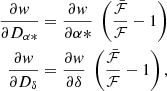
Under the effect of the gravitational force, the two components of a binary are accelerated towards each other. If they cannot be resolved and the photocentre does not coincide with the barycentre, the apparent motion of their photocentre is accelerated; when the orbital period is much longer than the time interval covered by the observations, the acceleration is nearly constant in intensity and direction. These physical considerations are at the origin of the constant acceleration model. Each coordinate of the photocentre varies with time according to a parabola. However, fitting a parabola to the set of observations means setting the mid-mission position of the star as given by the first two terms of the solution, so that it is tangent to the parabola, and therefore far from the mean position of the star. To provide a position closer to the mean position of the star, we followed the method explained in the HIPPARCOS catalogue (ESA 1997, Vol. 1, Sect. 2.3.3), and the partial derivatives of the abscissa with respect to the acceleration, (gα*, gδ), are given by the following equations:
![Mathematical equation: $$ \begin{aligned}&\frac{\partial w}{\partial g_{\alpha *}} = \frac{1}{2} \frac{\partial w}{\partial \alpha *} \; \left[ (t-T)^2 - \frac{\Delta T^2}{3} \right] \nonumber \\&\frac{\partial w}{\partial g_\delta } = \frac{1}{2} \frac{\partial w}{\partial \delta } \; \left[ (t-T)^2 - \frac{\Delta T^2}{3} \right] , \end{aligned} $$](/articles/aa/full_html/2023/06/aa43969-22/aa43969-22-eq17.gif) (6)
(6)
where T is 2016.0 as in Sect. 3.2, and ΔT is half the time interval covered by the observation of the star. For simplicity, the same value of ΔT was assumed for all stars, and we adopted half the time between the start of the Gaia science mission and the last DR3 observation, which, according to the information available when the software was finalised, lead to ΔT = 1035/2 = 517.5 d, or 1.417 yr. However, this is an overestimation: the last observation of the DR3 was made on 28 May 2017, three days later than we had assumed, but, on the other hand, the astrometric data of the first month of the Gaia scientific mission were not taken into account (Lindegren et al. 2021). Moreover, the actual duration covered by the observations of a star is necessarily shorter than the duration covered by all the observations. For all these reasons, ΔT should be rather of the order of 470 days. However, the resulting shift in the mean position is very small: 0.06 mas times the acceleration in mas yr−2. The significance of the constant acceleration model is defined from the acceleration vector and is derived from Eq. (3), as explained in Sect. 2.3.2.
4.2. The variable acceleration model
When the gravitational force is significantly changing over the duration of the mission, but when the orbital period is still much longer than the observation time span, the time derivative of the acceleration,  , is added to the parameters of the model. However, the introduction of these parameters could modify the proper motion of the star. In order to derive a proper motion corresponding to the average displacement of the photocentre during the mission, the partial derivatives of the abscissa with respect to
  and
and  are given by the equations:
![Mathematical equation: $$ \begin{aligned} \begin{array}{@ll} \frac{\partial w}{\partial \dot{g}_{\alpha *}} = \frac{1}{6} \frac{\partial w}{\partial \alpha *} \; \left[ (t-T)^2 - \Delta T^2 \right] (t-T)&\\ \\ \frac{\partial w}{\partial \dot{g}_\delta } = \frac{1}{6} \frac{\partial w}{\partial \delta } \; \left[ (t-T)^2 - \Delta T^2 \right] (t-T),&\end{array} \end{aligned} $$](/articles/aa/full_html/2023/06/aa43969-22/aa43969-22-eq21.gif) (7)
(7)
where ΔT is the same as in Sect. 4.1 above. We emphasise that the only effect of introducing ΔT is to produce a position and proper motion similar to that which would result from applying the single-star model. As acceleration models cannot locate the barycentre of a binary, these parameters are still affected by the orbital motion of the photocentre relative to the barycentre.
The significance of the variable acceleration model is defined from the  vector. As above, this is derived from Eq. (3), as explained in Sect. 2.3.2. It is worth noting that the acceleration models are both linear models, and that the solutions are found by solving a system of linear equations by singular value decomposition.
In the HIPPARCOS reduction, the constant acceleration solution was considered as acceptable when the acceleration was significant, but the variable acceleration solution was always tried and, when significant, was preferred to the constant acceleration solution. We have kept this strategy, and, for that reason, the variable acceleration model was tried first. The variable acceleration solution was retained when it satisfied the conditions: s > 12 and F2 < 25. Otherwise, the constant acceleration solution was derived, and was accepted when it satisfied the same conditions. Because of this acceptance, no other models were tried. Therefore, acceleration solutions were retained for many binary stars with periods shorter than the duration of the Gaia mission. This choice was originally made to save computing time; this reason was no longer relevant at the time of processing the DR3, but the strategy remained unchanged because the risk of producing an orbit with an incorrect period was considered to be more serious than that of giving only a polynomial fit for a trajectory that could be described by an ellipse. This is a matter of judgement which may be considered questionable, and a different approach will probably be taken in the next data release.
4.3. Selection of the acceleration solutions
To delimit a domain of acceptance of the solutions, for both acceleration models, we consider the true acceleration projected on the sky. This latter is referred to as Γ in the following and is derived from the equation:
 (8)
(8)
When the apparent acceleration is expressed in mas yr−2 and when the parallax is in mas, Γ is obtained in au yr−2. In order to estimate a maximum value for Γ, we consider a bright star with a dark companion, so that the acceleration of the photocentre is that of the bright star. Applying the law of gravitation, and assuming that the distance between the components is approximately equal to the semi-major axis of the orbit of the bright star around the companion, we deduce from Kepler’s third law that the acceleration is then:
 (9)
(9)
where P is the period, M the mass of the bright star, and q the mass ratio, that is, the ratio between the mass of the dark companion and M.
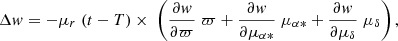
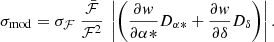
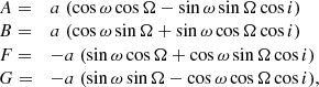
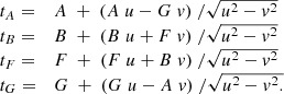
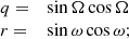
An upper limit on Γ is obtained when the bright star is a giant solar-mass star with a companion still on the main sequence or on the subgiant branch, with q slightly less than 1, and when the period is twice the duration of the Gaia mission. Such a system is not frequent, but is not exceptional in a sample bounded by a limit in magnitude. With a period of 5.7 yr, the acceleration may be as large as about 2.4 au yr−2 for a circular orbit; over half a period, the average acceleration can then be as high as 2.0 au yr−2. However, this result is a rough estimate: we have neglected the eccentricity, which will produce a larger acceleration near the periastron, and we have assumed a period much longer than the duration of the mission, whereas we know that many solutions are for shorter periods. Considering the distribution of values obtained from the solutions (see Figs. 2a and b), we see a concentration below Γ = 3 au yr−2, which we adopt as the limit for an acceptable acceleration solution. Stars whose acceleration is really beyond this limit are certainly very rare, but they are also objects of great scientific interest, such as binaries with a massive dark component, and for this reason we do not reject them directly.
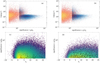 |
Fig. 2. Selection of the acceleration solutions. The left-hand panels correspond to solutions with constant acceleration, and those on the right to those with variable acceleration. Panels (a) and (b): significance vs. acceleration diagrams from a processing trial without the selection based on parallax error. The solutions with F2 below the final threshold are in blue, while those above are in orange. The solutions of 5 < s < 12 were accepted in the absence of better solutions from another model, while the others were immediately accepted when s > 12 and F2 was below 22 (for constant acceleration solutions) or 25 (for variable acceleration solutions). The number of solutions with a mean acceleration Γ > 3 au yr−2 falls off when the significance exceeds 20. Panels (c) and (d): the F2 vs. s diagrams of the solutions finally selected in the post-processing. The black dots are the remaining solutions with Γ > 3 au yr−2; they still correspond to the smallest significances, but this is essentially due to the filtering based on the parallax error. |
The following three conditions were introduced to restrict the proportion of Γ larger than this limit: (1) As mentioned in Sect. 4.2 above, the main processing was performed with the threshold s > 12 for direct acceptance and s > 5 for the alternative solutions. In addition, conditions based on the significance of the parallax were introduced for both levels: ϖ/σϖ > 1.2 s1.05 for the constant acceleration model, and ϖ/σϖ > 2.1 s1.05 for the variable acceleration model. These conditions were set because they very effectively reduce the number of high accelerations; it is worth noting that they are not criteria based on the quality of the solutions: reading them from right to left, they both mean that, for a given distance, the most significant solutions are rejected. This results in rejecting the largest accelerations because many of them are highly significant, and their occurrence rate is therefore artificially reduced. However, it was necessary to apply these criteria to avoid too much pollution from partially resolved double stars. Another beneficial consequence of this filter is that the short-period binaries whose acceleration solution was rejected in this way were able to have an orbital solution. Including alternative solutions, the main processing yielded 808 992 constant acceleration solutions and 569 022 variable acceleration solutions. These solutions must be filtered in the post-processing to keep only those that seem most likely to be real. (2) The significance, s, must be over 20 for both acceleration models. (3) The goodness of fit, F2, must be below 22 for the constant acceleration model, and below 25 for the variable acceleration model. The limit is more severe for the constant acceleration solutions so that the sequences of the Hertzsprung–Russel (HR) diagrams deduced from the parallaxes of these solutions are always thinner than those deduced from the single-star model. Conditions (2) and (3) reduced the number of solutions to 246 798 for constant accelerations, and 91 227 for variable accelerations.
The two lower panels of Fig. 2 show the distributions of the selected solutions in the F2 vs. s diagrams. Thanks to the parallax filtering (item (1) above), the solutions with Γ > 3 au yr−2 are very rare: 0.03% of the constant acceleration solutions, and 0.3% for the variable accelerations. If filters (2) and (3) are applied to a test sample unaffected by filter (1), the proportions of large Γ are 3.1% and 5.6% respectively. Unless one is prepared to sacrifice the vast majority of solutions, these high rates resist the quality criteria we have tried; this issue is discussed further in Sect. 7, taking into account the results of independent investigations. Several origins have been considered for the high acceleration solutions: short-period binaries, partially resolved binaries, or outlier astrometric measurements. We can only conclude that the stars with acceleration solutions are most likely genuine binaries, but the physical interpretation of the accelerations is hazardous.
5. Orbital solutions
An orbital solution is calculated when the orbit has been observed either in its entirety or over a sufficient portion to extrapolate the missing part. The general case concerns elliptical orbits; circular orbits are described by adapting it.
5.1. Calculation of the orbital solutions
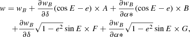
The abscissa of an unresolved astrometric binary can be written as in the following equation:
 (10)
(10)
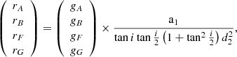
where wB is the abscissa of the barycentre, which is given by the single-star model, A, B, F, and G are the Thiele-Innes (TI) elements, whose definition is given in Eq. (A.1), e is the eccentricity of the orbit, and E is the eccentric anomaly. E depends on the observation epoch, but also on the orbital period, P, on e, and on the periastron epoch, T0, and so the model is finally based on 12 unknowns: the five parameters of the single-star solution, and A, B, F, G, P, e, and T0; the partial derivatives of w with respect to the TI elements are given in Eq. (10), and those with respect to P, e, and T0 can be found in Goldin & Makarov (2006).
The derivation of the orbital solutions is based on the Levenberg–Marquardt algorithm, but this can only lead to the solution if it starts from a good starting point. In practice, a calculation starting from e = 0 often leads to the right result if the period tested is close to the actual period, but scanning a grid covering the space of P, e, and T0 is still necessary for finding the solution. The period range tried is from 10 days to the duration covered by the observations of the star divided by 0.6. The solutions are calculated and published in terms of TI elements, but the calculation of the elements usually used to describe an orbit, which are the so-called Campbell elements (semi-major axis, inclination of the orbit, position angle of the ascending node, and periastron longitude), is presented in Appendix A, where the calculations of their uncertainties are also given. The extension of this calculation to the Thiele-Innes elements introduced by both astrometric and spectroscopic orbits is presented in Appendix B.
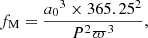
The significance of the orbital model is defined as the semi-major axis of the orbit, a0, divided by its uncertainty. This definition of the significance was adopted because a significant orbit is expected to have a large semi-major axis, when, on the contrary, an orbit with a semi-major axis close to or smaller than its uncertainty may be obtained for a single star. The semi-major axis is not explicitly a parameter of the orbital model that we have used, but it may be derived from the TI elements thanks to Eq. (A.2). Its uncertainty is derived from Eqs. (A.7) and (A.8).
5.2. Pseudo-circular and circular orbital solutions
Rare orbits (eight in total) have been directly calculated as circular and are given with e = 0. These calculations required special arrangements, which were also adopted for orbits with very small eccentricities, as explained below.
Preliminary calculations showed that the eccentricities below 0.006 were all at least three times smaller than their uncertainties. For such solutions, the uncertainties of the TI elements are also often very large, as is the uncertainty of T0, which can be larger than the period. These anomalies arise from the indeterminacy of the position of the periastron, affecting the TI elements through their dependence on the longitude of the periastron, ω (see Eq. (A.1)). They do not affect the validity of the solution, for which the Campbell elements calculated as explained in Appendix A have correct uncertainties, except for ω, whose uncertainty far exceeds 2π; however, they may confuse the user.
In order to limit these effects, orbits with an eccentricity of less than 0.0005 were ‘pseudo-circularised’ in the following way: The Campbell elements were derived, and the periastron longitude, ω, was set to zero in order to place the periastron on the ascending node. Therefore, the periastron epoch, T0, was advanced by subtracting the time interval corresponding to the orbit section between the ascending node and the initial periastron, which for a circular orbit is P × ω/(2π). As the initial orbit is not circular, this formula is an approximation that is only possible for very small eccentricities; this is why it was only done for e < 0.0005. The TI elements were then recalculated, keeping the semi-major axis, orbit inclination, and line-of-nodes position angle of the initial solution.
After these transformations, the solution is based on only ten unknowns: e is fixed, and only three of the four TI elements remain, because ω = 0 implies that G = −AF/B, or F = −BG/A. Therefore, G was no longer considered as an unknown provided that |B|> 10−5 mas. Otherwise, it was F that had to be removed, but this did not happen in practice. Thus, the solution variance-covariance matrix was recalculated for the ten selected unknowns. This 10 × 10 matrix was inserted into the 12 × 12 matrix of orbital solutions, setting the unnecessary terms to zero.
In the end, this gives quite reasonable uncertainties for the TI elements and for T0. However, the solution will give an uncertainty and correlation terms that are zero for G, which is wrong and needs to be corrected in order to deduce the uncertainties of Campbell’s elements as explained in Appendix A. The uncertainty of G, σG, is derived from the equation:
![Mathematical equation: $$ \begin{aligned}&\sigma _G = |G| \left[\left(\frac{\sigma _A}{A}\right)^2 + \left(\frac{\sigma _B}{B}\right)^2 + \left(\frac{\sigma _F}{F}\right)^2 \right.\nonumber \\&\qquad \left. + 2\left(\frac{\rho _{AB}\sigma _A\sigma _B}{AB} + \frac{\rho _{AF}\sigma _A\sigma _F}{AF} + \frac{\rho _{BF}\sigma _B\sigma _F}{BF}\right)\right]^{1/2}. \end{aligned} $$](/articles/aa/full_html/2023/06/aa43969-22/aa43969-22-eq26.gif) (11)
(11)
The correlation coefficients relating G to the other TI elements are:
 (12)
(12)
These modifications must also be made to circular orbits if the uncertainties of their Campbell elements are to be calculated.
5.3. Selection of the orbital solutions
The orbital solutions were first selected according to the thresholds set out in Sect. 2.3.2, the significance being calculated as explained in the previous section. In order to identify doubtful solutions, we took the mass function into account, which is derived from:
 (13)
(13)
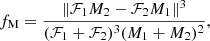
where P is the period in days, and where a0 and ϖ are in the same units; fM is therefore obtained in solar masses. Taking into account that a0 refers to the orbit of the photocentre, the third Kepler law gives the following expression:
 (14)
(14)
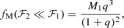
where ℱ1 and ℱ2 are the photometric fluxes of the brightest and of the faintest component, respectively, and M refers to the masses. When ℱ2 is negligible compared to ℱ1, this equation becomes:
 (15)
(15)
where q = M2/M1 and where the index ‘1’ refers to the brightest component.
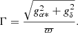
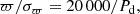
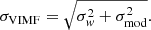
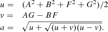
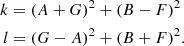
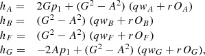
Panel a of Fig. 3 shows the period vs. mass function diagram. There are two kinds of false solutions: First of all, solutions of fM > 0.3 M⊙. This limit appears rather large for dwarf stars, but is roughly acceptable for binaries with a giant component and a component still close to the main sequence, or for a triple system with a massive pair as a secondary component. The second kind are solutions with particular periods, which probably depend on the 63-day precession period of the satellite. These solutions usually have a very large mass function, but they descend sufficiently into the small fM range to contaminate plausible solutions.
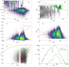 |
Fig. 3. Selection of the astrometric orbital solutions. The first row refers to the solution obtained from a processing trial without the selection based on parallax error. (a): period vs. mass function diagram, showing a clump of plausible solutions, bounded by fM ≈ 0.3 M⊙, and various sequences, organised around particular periods, which cross the clump and extend well beyond. (b): period vs. ‘parallax significance’. The solutions with fM < 0.3 M⊙ are in green, and the large fM, which are well clustered around the same periods as in panel (a), are in black. The line is the limit ϖ/σϖ = 20 000/Pd, which was implemented in the main processing to discard the dubious solutions. The second row shows the density map diagrams used to set up the post-processing filters to remove the concentrations still existing over specific periods. (c): period–eccentricity uncertainty diagram; solutions above the red line were rejected. (d): period–significance diagram; solutions below the red line were rejected. The third row shows properties of the DR3 solutions eventually selected after applying the post-processing filters. (e): the period–eccentricity diagram; the black curve is the maximum eccentricity assuming that the periods shorter than 10 days are circularised. The black dots are the solutions with fM > 0.3 M⊙. The astrometric-only orbital solutions are in green, while the solutions confirmed by a spectroscopic SB1 orbit from Gaia are in purple. (f): histogram of periods; the proportion of solutions with mass function above 0.3 solar masses, in black, increases with period, as the gap between these solutions and the totality, in green, is reduced (in order to highlight possible overdensities, the step size of the green histogram is very fine; to avoid fluctuations in counts from small numbers, the black histogram was plotted by merging the count intervals into clusters of four, and giving the mean value for each cluster). |
A large part of the last category of false solutions was discarded by using a filter based on the parallax significance, as indicated in Fig. 3b. This filter consists of selecting only the solutions that satisfy the following condition:
 (16)
(16)
and it allowed us to keep 179 234 astrometric orbits as a result of the main processing.
Although the filter of Eq. (16) has rejected most of the large mass function solutions, a few concentrations around particular periods still persist in the processing results (Figs. 3c and d). Most of these remaining false solutions were eliminated in the post-processing, where only solutions satisfying the following two filters were selected: a filter based on the quality of the eccentricity: σe < 0.079lnP − 0.244, where P is in days; and a filter based on the significance:  , where P is again in days.
After these operations, about 166 500 orbits were retained, and the concentrations along particular periods all disappeared, as shown in Fig. 3e. Moreover, very few orbits have eccentricities beyond the ten-day circularisation limit, calculated according to Halbwachs et al. (2005). The proportion of fM > 0.3 M⊙ is now about 1%, but it can be seen in Fig. 3f that it increases considerably with period: for example, it is only 0.2% for periods of less than 1 year, but reaches 3.3% for periods longer than 1000 days.
Subsequently, all the main processing astrometric orbits were compared to the SB1 spectroscopic orbits derived from Gaia radial velocities (Gosset et al., in prep.). The matching of the orbits of the two types resulted in nearly 30 950 combined orbits, of which about 2470 were recovered after having been rejected by the post-processing. At the same time, almost 3500 post-processing orbital solutions were rejected by the validation (Babusiaux et al. 2023), or discarded as redundant with solutions obtained with Markov chain Monte Carlo and Genetic Algorithms (Holl et al. 2023). In the end, our contribution to the DR3 astrometric orbital solutions amounts to nearly 165 500 orbits.
6. The variability-induced movers
The variability-induced movers (VIMs) were first described by Wielen (1996). These are defined as unresolved binary systems containing one photometrically variable component. The result is a photocentre which is moving between the components in accordance with fluctuations in the total brightness of the system. Simultaneously, it is following the orbital motion, if this is perceptible over the duration of the mission. Several types of VIM were expected from the Gaia astrometric and photometric measurements: when the orbital motion is not perceptible, the system is a fixed VIM (VIMF hereafter). When the orbital motion appears to be a motion of the components relative to each other, in a straight line and at constant velocity, the system is a VIM with linear motion, or VIML. This is followed by VIM with acceleration (constant or variable; VIMA), and then VIM with orbital motion (VIMO). Only VIMFs are described in detail below, as the others could not be included in the DR3.
6.1. The VIM with fixed components model
The additional parameters specific to the VIMF model are the coordinates of the photocentre, (Dα*, Dδ), measured from the variable component when the total photometric flux of the system is equal to a reference flux, noted  . In practice,
  is the median flux of all transits of the system. The partial derivatives of the abscissa with respect to Dα* an Dδ are given by the following equations:
 (17)
(17)
where ℱ is the photometric flux of the transit. Therefore, the position of the system and its proper motion also apply to the photocentre when the total flux is  .
.
The parameters of the VIMF model are therefore derived from a linear system that is solved by singular value decomposition, but the uncertainty of each transit requires a dedicated calculation, because it depends on the astrometric uncertainty of the measured abscissa, σw, but also on the uncertainty of the photometric flux, σF, on which an error from the model depends. For each transit, this error, σmod, is calculated from the equation:
 (18)
(18)
The total uncertainty of transit is then given by the equation:
 (19)
(19)
The σVIMF uncertainties are used to derive any VIMF solution, as well as F2 and the correction coefficient c as explained in Sect. 2.3.1. As σVIMF depends on Dα* and Dδ, and thus on the VIMF solution, the calculation is iterative and the VIMF model cannot be considered strictly linear. The significance of the solution is defined from the modulus of the (Dα*, Dδ) vector, as explained in Sect. 2.3.2. As far as the VIML model is concerned hereafter, suffice it to say that it has two more parameters, which are the time derivatives of Dα* and Dδ.
6.2. Selection of the VIMF solutions
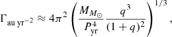
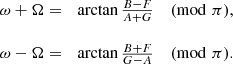
The main criterion we have for estimating whether or not a VIMF solution is plausible is the apparent distance D, which separates the median photocentre from the variable component. As the resolution of Gaia is at least 180 mas (Lindegren et al. 2021) and the components of a VIM should never be separated, D must remain under a limit of no more than 100 mas; we are therefore looking for quality criteria here such that this condition is met.
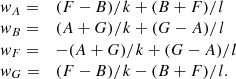
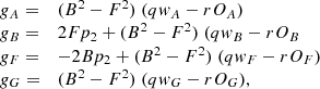
The F2 vs. D and significance vs. D diagrams obtained after a first processing trial do not immediately show any limits in F2 or significance that would allow almost only D < 100 mas. Fortunately, a selection becomes possible when we consider the ‘parallax significance’, that is, the quantity ϖ/σϖ. It is clear from Fig. 4 that the selection of solutions of parallax significance greater than 30 rejects most excessive values of D. Therefore, this criterion was applied in the main processing, in addition to the criteria s > 12 and F2 < 25. As before, the criteria for selecting alternative solutions were s > 5 and F2 less than that of the alternative solution that may have already been selected.
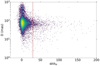 |
Fig. 4. ‘Parallax significance’ vs. D diagram of VIMF solutions obtained from a processing trial; most false solutions of D > 100 mas are eliminated if the selection criterion ϖ/σϖ > 30 (to the right of the vertical red line) is applied. |
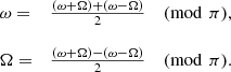
We obtained 2508 VIMF solutions from the main processing. The F2 vs. D diagram of these stars is shown in Fig. 5a. As for the previous models, solutions with F2 higher than 25 seem doubtful, because the proportion of large D values in them increases, and, more strikingly, small D values become increasingly rare as F2 increases. These solutions are therefore rejected, which leaves 1660 solutions. The significance vs. D diagram of these solutions shows a large scatter of D values when significance is below 20, and this scatter is exacerbated below 12. However, the threshold was set at 20 as a precaution. Beyond that, D increases with D/σD (Fig. 5b), which corresponds to a value of σD that is approximately constant and close to one-tenth of a milliarcsecond, which seems acceptable.
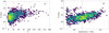 |
Fig. 5. Post-processing filtering of the VIMF solutions. Panel (a): F2 vs. D diagram of the 2508 solutions obtained from the main processing. The proportion of large D, and therefore false solutions, increases gradually beyond F2 = 25, to the right of the vertical red line. Panel (b): significance vs. D diagram of the 1660 solutions with F2 < 25; acceptable solutions cluster on a sequence of D increasing with significance; abnormally large D solutions are rejected by restricting to significances greater than 20 (to the right of the vertical red line), leaving a final selection of 869 solutions. |
The 869 retained VIMF solutions following the above processing have distances D below 40 mas, with three exceptions: three solutions of significance close to 100, for which D is 55, 56, and 101 mas. These values are not unrealistic, and it seems possible that all VIMF solutions are valid. Unfortunately, this may also be due to the low effectiveness of using D to point out dubious solutions, as the application of other VIM models has shown below.
6.3. The other VIM models
As explained at the beginning of this section, four other VIM models were tried, from VIML to VIMO. Contrary to the VIMF model, the parameters of these models allow the estimation of a minimum value for the mass of the systems. The result was devastating: for all these models, the minimum masses are concentrated between 10 and 10 000 M⊙. We therefore decided to remove these models from the mass processing cascade.
7. Discussion and conclusion
This first publication of astrometric binaries of different types observed by Gaia was made under difficult conditions, because the uncertainties of the measurements were often highly underestimated. However, we were able to calculate hundreds of thousands of reliable solutions by keeping the weights of the observations and correcting the uncertainties. Nevertheless, this was done at the cost of a drastic selection based on very high quality criteria, and it would be difficult to use the selected solutions to deduce the statistical properties of binary stars, as the sample is incomplete and biased.
Because of the cascade structure that leads to the testing of different models, we may have retained solutions by direct acceptance that would have been superseded by another model had it been tried. This choice has the advantage of preserving the quality of the orbital solutions, by assigning acceleration solutions to partially resolved double stars that would have been processed despite the filters set up to reject them. However, it was done at the expense of the completeness of the orbital solutions, and it is likely that some acceleration solutions actually correspond to binaries with periods short enough to have an orbital solution. Moreover, the quality criteria alone could not bring the acceleration solutions to a reasonable rate of high acceleration. Ulrich Bastian studied this problem long after the post-processing was done, and he estimated that constant acceleration solutions are only highly reliable when the parallax is greater than 5 mas. This criterion leaves only 15 000 solutions, but none with acceleration greater than 3 au yr−2. When only quality criteria are applied, that is, when criterion (1) of Sect. 4.3 is not applied, the restriction to parallaxes greater than 5 mas reduces the Γ > 3 au yr−2 rate from 3.1% to less than 1%; this confirms the effectiveness of this extremely drastic selection. For future data releases, it is hoped that the treatment of partially resolved double stars – as well as testing all astrometric models and choosing the one that is most compatible with the data – will allow a wider selection of acceleration solutions.
The selection of orbital solutions was particularly severe in order to reject orbits that are concentrated in certain periods, which are likely to be produced by the satellite’s scanning law. Despite these difficulties, about 165 500 astrometric orbits were finally selected in DR3. The periods of the false orbits should be different in the following data releases, as the precession spin has been reversed during the last 6 months of observations, which will be part of the DR4; however, if these noise-induced orbits do not disappear at this time, they could be more difficult to detect, being distributed over a larger number of periods. Furthermore, the lack of one-year periods, which comes from a degeneracy between parallactic and orbital motion, is expected to remain.
The acceleration and orbital models apply to unresolved binaries with either components that do not vary photometrically, or one component that is always much brighter than the other. This limits their interest in the study of young stars, or more generally, pulsating stars. VIM models extend the scientific scope of astrometric binaries, provided that only one of the components is photometrically variable. Unfortunately, the number of VIM solutions appears to be very modest, numbering only a few hundred, limited to the VIMs with fixed components. This rarity is partly due to the fact that the model has only been tried at the end of the cascade, and we do not know how many acceptable VIM solutions were lost due to the acceptance of a solution of another type.
When both components are variable, the VIM solution can be very degraded: When the brightnesses of the two stars vary in the same direction, the displacement of the photocentre can be very small while the brightness of the system varies greatly; for the VIMF model, this is interpreted as a short D distance. Conversely, if the brightness of one component increases while that of the other decreases, the fluctuation in total brightness may be small while the photocentre displacement is large. As the luminosities of the components do not generally vary in phase, one can expect VIMF solutions of large χ2, and therefore large F2, with D values that can be minimal or, on the contrary, very large. A large χ2 leads to a decrease in significance, thanks to the coefficient c of Eq. (2), and, as a result, the pollution of VIMF solutions by systems whose two components are photometrically variable will be limited thanks to the high acceptance thresholds that have been adopted.
Another difference between VIMFs and other solutions is that the selection could only be adjusted on the basis of the median distance between the photocentre and the photometric variable component, excluding any dynamic criteria. Therefore, these solutions should be considered with caution. In turn, it is possible that some acceleration or orbital solutions have been assigned to objects that should have received a VIM solution. However, these cases are too rare to constitute detectable pollution: Gaia Collaboration (2023) showed that, statistically, the proper motions of acceleration solutions are affected by orbital motion, which would not be the case for VIMFs. Similarly, if VIMFs receive an orbital solution, the inclination of the solution must be 90 deg, and the distribution of inclinations does not show an excess for this value.
Despite these limitations raised above, DR3 represents a major step forward in the field of binary stars. The hundreds of thousands of new astrometric orbits will be of considerable importance in the future, compared to the less than 3000 visual binary star orbits in the Sixth Catalog of Orbits of Visual Binary Stars1. Such a change of scale could open a new era in the statistical study of binary stars, especially if the next data releases are less affected by selection effects. Instead of looking at the properties of pairs with a primary component of a given type, it may be possible to consider pairs with a given total mass. Such an approach would shed new light on the star formation process, provided that the many biases affecting binary selection are taken into account.
Acknowledgments
This work is part of the reduction of the Gaia satellite observations (https://www.cosmos.esa.int/gaia). The Gaia space mission is operated by the European Space Agency, and the data are being processed by the Gaia Data Processing and Analysis Consortium (DPAC, https://www.cosmos.esa.int/web/gaia/dpac/consortium). The Gaia archive website is https://archives.esac.esa.int/gaia. Funding for the DPAC is provided by national institutions, in particular the institutions participating in the Gaia MultiLateral Agreement (MLA). We acknowledge for the financial support of the french “Centre National d’études spatiales” (CNES) and of the BELgian federal Science Policy Office (BELSPO) through a PROgramme de Développement d’Expériences scientifiques (PRODEX). Over the two decades that it took to develop the calculation methods and write the software, we benefited from the contributions of Sylvie Jancart, Rémy Onsay, Didier Pelat and Patrick Gempin. We also received constant support from François Mignard and Alain Jorissen. The acceptability of acceleration solutions was discussed with Ulrich Bastian and Lennart Lindegren, using data produced by Sergei Klioner and Hagen Steidelmüller. Finally, we are grateful to Michael Biermann and to an anonymous referee for their careful reading of the manuscript and the relevance of their comments.
References
- Babusiaux, C., Fabricius, C., Khanna, S., et al. 2023, A&A, 674, A32 (Gaia DR3 SI) [NASA ADS] [CrossRef] [EDP Sciences] [Google Scholar]
- Binnendijk, L. 1960, Properties of Double Stars; A Survey of Parallaxes and Orbits (Philadelphia: University of Pennsylvania Press) [CrossRef] [Google Scholar]
- Dravins, D., Lindegren, L., & Madsen, S. 1999, A&A, 348, 1040 [NASA ADS] [Google Scholar]
- ESA 1997, The Hipparcos and Tycho Catalogue SP-1200 [Google Scholar]
- Gaia Collaboration (Brown, A. G. A., et al.) 2021, A&A, 649, A1 [NASA ADS] [CrossRef] [EDP Sciences] [Google Scholar]
- Gaia Collaboration (Arenou, F., et al.) 2023, A&A, 674, A34 (Gaia DR3 SI) [CrossRef] [EDP Sciences] [Google Scholar]
- Goldin, A., & Makarov, V. V. 2006, ApJS, 166, 341 [NASA ADS] [CrossRef] [Google Scholar]
- Halbwachs, J.-L. 2009, MNRAS, 394, 1075 [CrossRef] [Google Scholar]
- Halbwachs, J.-L., Mayor, M., & Udry, S. 2005, A&A, 431, 1129 [NASA ADS] [CrossRef] [EDP Sciences] [Google Scholar]
- Heintz, W. D. 1978, Double Stars (Dordrecht: Reidel) [CrossRef] [Google Scholar]
- Holl, B., Sozzetti, A., Sahlmann, J., et al. 2023, A&A, 674, A10 (Gaia DR3 SI) [NASA ADS] [CrossRef] [EDP Sciences] [Google Scholar]
- Lindegren, L., & Dravins, D. 2003, A&A, 401, 1185 [NASA ADS] [CrossRef] [EDP Sciences] [Google Scholar]
- Lindegren, L., Klioner, S. A., Hernández, J., et al. 2021, A&A, 649, A2 [EDP Sciences] [Google Scholar]
- Riello, M., De Angeli, F., Evans, D. W., et al. 2021, A&A, 649, A3 [NASA ADS] [CrossRef] [EDP Sciences] [Google Scholar]
- Stuart, A., & Ord, K. 1994, Kendall’s Advanced Theory of Statistics (London: Edward Arnold), 1 [Google Scholar]
- Wielen, R. 1996, A&A, 314, 679 [NASA ADS] [Google Scholar]
Appendix A: Conversion of Thiele-Innes elements (A, B, F, G) into Campbell elements (a, i, Ω, ω) and calculation of the uncertainties
The Thiele-Innes (TI) elements A, B, F, and G are given by the following equations (Binnendijk 1960; Heintz 1978):
 (A.1)
(A.1)
where a, i, Ω, and ω are the Campbell elements. The definitions of these elements and their calculations from A, B, F, and G are given hereafter:
-
a (or a0 for a photocentric orbit) is the semi-major axis of the orbit, in the same unit as the TI elements.
-
i is the inclination of the orbit, i.e. the angle between the orbital plane and the plane of the sky. i ∈ [0, π/2] when the orbital motion is in the direct sense, and i ∈ [π/2, π] when the photocentre is revolving around the barycentre in a clockwise direction.
-
Ω is the position angle of the ascending node. Here, the ascending node is taken as the intersection between the orbital plane and the plane of the sky in the direction where the right ascension is increasing. Therefore, Ω ∈ [0, π].
-
ω is the periastron longitude measured in the orbital plane from the ascending node defined above. ω is measured in the sense of the orbital motion.
Binnendijk (1960) gives the following method for converting TI elements into Campbell elements:
The semi-major axis a, is derived from:
 (A.2)
(A.2)
The angles Ω and ω are derived simultaneously. Preliminary estimates, between −π and π, are derived as follows:
 (A.3)
(A.3)
The exact values of ω + Ω are obtained (mod 2π), taking into account that sin(ω + Ω) and (B − F) have the same sign. Similarly, sin(ω − Ω) has the same sign as ( − B − F). ω and Ω are then derived from the equations:
 (A.4)
(A.4)
When Ω is negative, π must still be added to both Ω and ω. After that, a correction of 2π may still be applied in order to meet the conditions Ω ∈ [0, π] and ω ∈ [0, 2π].
To derive the inclination i, we first need to calculate two intermediate terms, called d1 and d2 hereafter:
 (A.5)
(A.5)
In order to obtain the value of i, the calculation is different depending on whether d1 is greater than d2, or the reverse:
 (A.6)
(A.6)
The uncertainties of a, i, Ω, and ω are derived by differentiating the equations above, and by taking into account error propagation. Hereafter, we denote σp the error on element p and cov(X,Y) the term of the variance covariance matrix of the solution linking the elements X and Y, i.e. cov(X, Y) = ρXYσXσY, where ρXY is the correlation coefficient between X and Y. The uncertainties are then given by the equations below.
To derive the uncertainty of a, the following intermediate terms must be calculated from u and v derived in Eq. (A.2):
 (A.7)
(A.7)
The uncertainty of the semi-major axis is then:
![Mathematical equation: $$ \begin{aligned} \begin{array}{ll} \sigma _a = \frac{1}{2a} \; \times \; [&t_A^2 \sigma _A^2 + t_B^2 \sigma _B^2 + t_F^2 \sigma _F^2 + t_G^2 \sigma _G^2 \\&+ \; 2 t_A t_B \mathrm{cov} (A,B) + 2 t_A t_F \mathrm{cov} (A,F) \\&+ \; 2 t_A t_G \mathrm{cov} (A,G) + 2 t_B t_F \mathrm{cov} (B,F) \\&+ \; 2 t_B t_G \mathrm{cov} (B,G) + 2 t_F t_G \mathrm{cov} (F,G) \; ]^{1/2}. \end{array} \end{aligned} $$](/articles/aa/full_html/2023/06/aa43969-22/aa43969-22-eq46.gif) (A.8)
(A.8)
The uncertainties of ω and Ω are also derived using dedicated intermediate terms. We first calculate the following:
 (A.9)
(A.9)
These terms are used to derive other intermediate terms dedicated to the calculation of the uncertainty of ω:
 (A.10)
The uncertainty of ω, σω is then derived with the following equation:
![Mathematical equation: $$ \begin{aligned} \begin{array}{ll} \sigma _\omega =&[ w_A^2 \sigma _A^2 + w_B^2 \sigma _B^2 + w_F^2 \sigma _F^2 + w_G^2 \sigma _G^2 \\&+ \; 2 \; ( \; w_A w_B \; \mathrm{cov} (A,B) + w_A w_F \; \mathrm{cov} (A,F) \\&+ w_A w_G \; \mathrm{cov} (A,G) + w_B w_F \; \mathrm{cov} (B,F) \\&+ w_B w_G \; \mathrm{cov} (B,G) + w_F w_G \; \mathrm{cov} (F,G) \; ) \; ]^{1/2} \; / \; 2. \end{array} \end{aligned} $$](/articles/aa/full_html/2023/06/aa43969-22/aa43969-22-eq49.gif) (A.11)
(A.11)
The terms from Eq. (A.9) are also used to compute the following intermediate terms, which are required to derive the uncertainty of Ω:
 (A.12)
The uncertainty of Ω is then:
![Mathematical equation: $$ \begin{aligned} \begin{array}{ll} \sigma _\Omega =&[ O_A^2 \sigma _A^2 + O_B^2 \sigma _B^2 + O_F^2 \sigma _F^2 + O_G^2 \sigma _G^2 \\&+ \; 2 \; ( \; O_A O_B \; \mathrm{cov} (A,B) + O_A O_F \; \mathrm{cov} (A,F) \\&+ O_A O_G \; \mathrm{cov} (A,G) + O_B O_F \; \mathrm{cov} (B,F) \\&+ O_B O_G \; \mathrm{cov} (B,G) + O_F O_G \; \mathrm{cov} (F,G) \; ) \; ]^{1/2} \; / \; 2. \end{array} \end{aligned} $$](/articles/aa/full_html/2023/06/aa43969-22/aa43969-22-eq51.gif) (A.13)
(A.13)
As in the derivation of i, the derivation of the uncertainty of the inclination depends on a comparison between d1 and d2, derived in Eq. (A.5) above.
σi is derived as follows. We first calculate the terms:
 (A.14)
if d1 ≥ d2, the continuation of the calculation is as explained hereafter. An extra term, p1, is added to q and r:
 (A.15)
The intermediate terms dedicated to the calculation of σi are then:
 (A.16)
and, still for d1 ≥ d2, σi is derived from the equation:
![Mathematical equation: $$ \begin{aligned} \begin{array}{ll} \sigma _i =&[ h_A^2 \sigma _A^2 + h_B^2 \sigma _B^2 + h_F^2 \sigma _F^2 + h_G^2 \sigma _G^2 \\&+ \; 2 \; ( \; h_A h_B \; \mathrm{cov} (A,B) + h_A h_F \; \mathrm{cov} (A,F) \\&+ h_A h_G \; \mathrm{cov} (A,G) + h_B h_F \; \mathrm{cov} (B,F) \\&+ h_B h_G \; \mathrm{cov} (B,G) + h_F h_G \; \mathrm{cov} (F,G) \; ) \; ]^{1/2} \\&/ \; [ \; ( \tan (i/2) + \tan ^3 (i/2)) \; d_1^2 \; ]. \end{array} \end{aligned} $$](/articles/aa/full_html/2023/06/aa43969-22/aa43969-22-eq55.gif) (A.17)
(A.17)
When d2 < d1, the additional term p2 is derived:
 (A.18)
The intermediate terms dedicated to the calculation of σi are now:
 (A.19)
and, still for d1 < d2, σi is derived from the equation:
![Mathematical equation: $$ \begin{aligned} \begin{array}{ll} \sigma _i =&[ g_A^2 \sigma _A^2 + g_B^2 \sigma _B^2 + g_F^2 \sigma _F^2 + g_G^2 \sigma _G^2 \\&+ \; 2 \; ( \; g_A g_B \; \mathrm{cov} (A,B) + g_A g_F \; \mathrm{cov} (A,F) \\&+ g_A g_G \; \mathrm{cov} (A,G) + g_B g_F \; \mathrm{cov} (B,F) \\&+ g_B g_G \; \mathrm{cov} (B,G) + g_F g_G \; \mathrm{cov} (F,G) \; ) \; ]^{1/2} \\&/ \; [ \; ( \tan (i/2) + \tan ^3 (i/2)) \; d_2^2 \; ]. \end{array} \end{aligned} $$](/articles/aa/full_html/2023/06/aa43969-22/aa43969-22-eq58.gif) (A.20)
(A.20)
The four Campbell elements and their uncertainties are therefore deduced from the solutions calculated in TI elements. However, it is not possible to estimate the correlation coefficients between the terms.
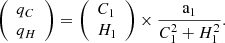
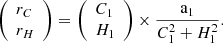
Appendix B: Conversion of Thiele-Innes elements (C1, H1) into elements (a1, ω1) and calculation of the uncertainties
The C1 and H1 elements are functions of the a1 and ω1 elements that come from the spectroscopic orbit:
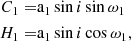 (B.1)
(B.1)
from which it appears that:
 (B.2)
(B.2)
knowing that sign(sin ω1) = sign(C1)and sign(cos ω1) = sign(H1).
ω1 must be approximately equal to either ω or ω + π. This ambiguity is due to differences in definition: ω is the longitude of the periastron of the photocentre orbit, which, in the absence of radial velocity, is measured from the node whose position angle is between 0 and π. For its part, ω1 is the longitude of the periastron of the orbit of the spectroscopically most visible component, measured from the node where this component moves away from the Sun. Therefore, the true orientation of the orbital plane will depend on the position of the photocentre with respect to the barycentre and the spectroscopic component: if the photocentre is assumed to be between the barycentre and the spectroscopic component, then the true ascending node and periastron of the astrometric orbit are marked by the same angles as those of the spectroscopic orbit. If ω and ω1 are significantly different, it is necessary to add ±π to ω to make them roughly coincide, and also to add π to Ω to take into account the change of reference node.
Alternatively, the photocentre may be opposite to the spectroscopic component (this may occur, for example, when the spectral type of the brightest component is very different from the templates used for spectroscopic reduction, so that the spectroscopic orbit corresponds to the least bright binary component). When this occurs, ω must be approximately equal to ω1 ± π. If it is not, ±π must be added to ω and π must be added to Ω for the orientation of the astrometric orbit to be completely defined.
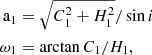
The calculation of the uncertainty of a1 depends on the values of d1 and d2, given by Eq. (A.5). When d1 ≥ d2, we compute the following terms:
 (B.3)
(B.3)
where hA, hB, hF, and hG are taken from Eq. (A.16), and
 (B.4)
(B.4)
The uncertainty σa1 is then calculated with equation:
![Mathematical equation: $$ \begin{aligned} \begin{array}{ll} \sigma _{\mathrm{a}_1} =&[q_A^2 \sigma _A^2 + q_B^2 \sigma _B^2 + q_F^2 \sigma _F^2 + q_G^2 \sigma _G^2 + q_C^2 \sigma _{C_1}^2 + q_H^2 \sigma _{H_1}^2 \\&+ \; 2 \; ( \; q_A q_B \; \mathrm{cov} (A,B) + q_A q_F \; \mathrm{cov} (A,F) \\&+ q_A q_G \; \mathrm{cov} (A,G) + q_A q_C \; \mathrm{cov} (A,C_1) \\&+ q_A q_H \; \mathrm{cov} (A,H_1) + q_B q_F \; \mathrm{cov} (B,F) \\&+ q_B q_G \; \mathrm{cov} (B,G) + q_B q_C \; \mathrm{cov} (B,C_1) \\&+ q_B q_H \; \mathrm{cov} (B,H_1) + q_F q_G \; \mathrm{cov} (F,G) \\&+ q_F q_C \; \mathrm{cov} (F,C_1) + q_F q_H \; \mathrm{cov} (F,H_1) \\&+ q_G q_C \; \mathrm{cov} (G,C_1) + q_G q_H \; \mathrm{cov} (G,H_1) \\&+ q_C q_H \; \mathrm{cov} (C_1,H_1) \; ) \; ]^{1/2}. \end{array} \end{aligned} $$](/articles/aa/full_html/2023/06/aa43969-22/aa43969-22-eq63.gif) (B.5)
(B.5)
When d2 > d1, these equations become:
 (B.6)
(B.6)
where gA, gB, gF, and gG are taken from Eq. (A.19), and
 (B.7)
(B.7)
The uncertainty σa1 is then calculated with the equation:
![Mathematical equation: $$ \begin{aligned} \begin{array}{ll} \sigma _{\mathrm{a}_1} =&[r_A^2 \sigma _A^2 + r_B^2 \sigma _B^2 + r_F^2 \sigma _F^2 + r_G^2 \sigma _G^2 + r_C^2 \sigma _{C_1}^2 + r_H^2 \sigma _{H_1}^2 \\&+ \; 2 \; ( \; r_A r_B \; \mathrm{cov} (A,B) + r_A r_F \; \mathrm{cov} (A,F) \\&+ r_A r_G \; \mathrm{cov} (A,G) + r_A r_C \; \mathrm{cov} (A,C_1) \\&+ r_A r_H \; \mathrm{cov} (A,H_1) + r_B r_F \; \mathrm{cov} (B,F) \\&+ r_B r_G \; \mathrm{cov} (B,G) + r_B r_C \; \mathrm{cov} (B,C_1) \\&+ r_B r_H \; \mathrm{cov} (B,H_1) + r_F r_G \; \mathrm{cov} (F,G) \\&+ r_F r_C \; \mathrm{cov} (F,C_1) + r_F r_H \; \mathrm{cov} (F,H_1) \\&+ r_G r_C \; \mathrm{cov} (G,C_1) + r_G r_H \; \mathrm{cov} (G,H_1) \\&+ r_C r_H \; \mathrm{cov} (C_1,H_1) \; ) \; ]^{1/2}. \end{array} \end{aligned} $$](/articles/aa/full_html/2023/06/aa43969-22/aa43969-22-eq66.gif) (B.8)
(B.8)
The uncertainty of ω1, σω1, is derived from:
![Mathematical equation: $$ \begin{aligned} \sigma _{\omega _1} = \frac{\cos ^2 \omega _1}{H_1^2} [H_1^2 \sigma _{C_1}^2 + C_1^2 \sigma _{H_1}^2 - 2 C_1 H_1 \; \mathrm{cov} (C_1,H_1)]^{1/2} .\end{aligned} $$](/articles/aa/full_html/2023/06/aa43969-22/aa43969-22-eq67.gif) (B.9)
(B.9)
All Tables
Properties of the different models and final conditions for the selection of solutions.
All Figures
|
Fig. 1. Overall organisation of the astrometric treatment of binary stars, as was eventually applied to the DR3. The cascade on the left side of the figure is the ‘main processing’ referred to hereafter. |
| In the text | |
|
Fig. 2. Selection of the acceleration solutions. The left-hand panels correspond to solutions with constant acceleration, and those on the right to those with variable acceleration. Panels (a) and (b): significance vs. acceleration diagrams from a processing trial without the selection based on parallax error. The solutions with F2 below the final threshold are in blue, while those above are in orange. The solutions of 5 < s < 12 were accepted in the absence of better solutions from another model, while the others were immediately accepted when s > 12 and F2 was below 22 (for constant acceleration solutions) or 25 (for variable acceleration solutions). The number of solutions with a mean acceleration Γ > 3 au yr−2 falls off when the significance exceeds 20. Panels (c) and (d): the F2 vs. s diagrams of the solutions finally selected in the post-processing. The black dots are the remaining solutions with Γ > 3 au yr−2; they still correspond to the smallest significances, but this is essentially due to the filtering based on the parallax error. |
| In the text | |
|
Fig. 3. Selection of the astrometric orbital solutions. The first row refers to the solution obtained from a processing trial without the selection based on parallax error. (a): period vs. mass function diagram, showing a clump of plausible solutions, bounded by fM ≈ 0.3 M⊙, and various sequences, organised around particular periods, which cross the clump and extend well beyond. (b): period vs. ‘parallax significance’. The solutions with fM < 0.3 M⊙ are in green, and the large fM, which are well clustered around the same periods as in panel (a), are in black. The line is the limit ϖ/σϖ = 20 000/Pd, which was implemented in the main processing to discard the dubious solutions. The second row shows the density map diagrams used to set up the post-processing filters to remove the concentrations still existing over specific periods. (c): period–eccentricity uncertainty diagram; solutions above the red line were rejected. (d): period–significance diagram; solutions below the red line were rejected. The third row shows properties of the DR3 solutions eventually selected after applying the post-processing filters. (e): the period–eccentricity diagram; the black curve is the maximum eccentricity assuming that the periods shorter than 10 days are circularised. The black dots are the solutions with fM > 0.3 M⊙. The astrometric-only orbital solutions are in green, while the solutions confirmed by a spectroscopic SB1 orbit from Gaia are in purple. (f): histogram of periods; the proportion of solutions with mass function above 0.3 solar masses, in black, increases with period, as the gap between these solutions and the totality, in green, is reduced (in order to highlight possible overdensities, the step size of the green histogram is very fine; to avoid fluctuations in counts from small numbers, the black histogram was plotted by merging the count intervals into clusters of four, and giving the mean value for each cluster). |
| In the text | |
|
Fig. 4. ‘Parallax significance’ vs. D diagram of VIMF solutions obtained from a processing trial; most false solutions of D > 100 mas are eliminated if the selection criterion ϖ/σϖ > 30 (to the right of the vertical red line) is applied. |
| In the text | |
|
Fig. 5. Post-processing filtering of the VIMF solutions. Panel (a): F2 vs. D diagram of the 2508 solutions obtained from the main processing. The proportion of large D, and therefore false solutions, increases gradually beyond F2 = 25, to the right of the vertical red line. Panel (b): significance vs. D diagram of the 1660 solutions with F2 < 25; acceptable solutions cluster on a sequence of D increasing with significance; abnormally large D solutions are rejected by restricting to significances greater than 20 (to the right of the vertical red line), leaving a final selection of 869 solutions. |
| In the text | |
Current usage metrics show cumulative count of Article Views (full-text article views including HTML views, PDF and ePub downloads, according to the available data) and Abstracts Views on Vision4Press platform.
Data correspond to usage on the plateform after 2015. The current usage metrics is available 48-96 hours after online publication and is updated daily on week days.
Initial download of the metrics may take a while.