| Issue |
A&A
Volume 673, May 2023
|
|
|---|---|---|
| Article Number | A35 | |
| Number of page(s) | 8 | |
| Section | Astronomical instrumentation | |
| DOI | https://doi.org/10.1051/0004-6361/202346230 | |
| Published online | 03 May 2023 | |
Designing wavelength sampling for Fabry–Pérot observations
Information-based spectral sampling
1
Institute of Theoretical Astrophysics, University of Oslo,
PO Box 1029
Blindern,
0315
Oslo,
Norway
e-mail: This email address is being protected from spambots. You need JavaScript enabled to view it.
2
Rosseland Centre for Solar Physics, University of Oslo,
PO Box 1029
Blindern,
0315
Oslo,
Norway
3
Institute for Solar Physics, Dept. of Astronomy, Stockholm University, AlbaNova University Centre,
10691
Stockholm,
Sweden
Received:
23
February
2023
Accepted:
22
March
2023
Abstract
Context. Fabry–Pérot interferometers (FPIs) have become very popular in solar observations because they offer a balance between cadence, spatial resolution, and spectral resolution through a careful design of the spectral sampling scheme according to the observational requirements of a given target. However, an efficient balance requires knowledge of the expected target conditions, the properties of the chosen spectral line, and the instrumental characteristics.
Aims. Our aim is to find a method that allows the optimal spectral sampling of FPI observations in a given spectral region to be found. The selected line positions must maximize the information content in the observation with a minimal number of points.
Methods. In this study, we propose a technique based on a sequential selection approach in which a neural network is used to predict the spectrum (or physical quantities, if the model is known) from the information at a few points. Only those points that contain relevant information and improve the model prediction are included in the sampling scheme.
Results. We have quantified the performance of the new sampling schemes by showing the lower errors in the model parameter reconstructions. The method adapts the separation of the points according to the spectral resolution of the instrument, the typical broadening of the spectral shape, and the typical Doppler velocities. The experiments that use the Ca II 8542 Å line show that the resulting wavelength scheme naturally places more points in the core than in the wings (by almost a factor of 4), consistent with the sensitivity of the spectral line at each wavelength interval. As a result, observations focused on magnetic field analysis should prioritize a denser grid near the core, while those focused on thermodynamic properties would benefit from a larger coverage. The method can also be used as an accurate interpolator to improve the inference of the magnetic field when using the weak-field approximation.
Conclusions. Overall, this method offers an objective approach for designing new instrumentation or observing proposals with customized configurations for specific targets. This is particularly relevant when studying highly dynamic events in the solar atmosphere with a cadence that preserves spectral coherence without sacrificing much information.
Key words: Sun: atmosphere / line: formation / methods: observational / Sun: activity / radiative transfer
© The Authors 2023
 Open Access article, published by EDP Sciences, under the terms of the Creative Commons Attribution License (https://creativecommons.org/licenses/by/4.0), which permits unrestricted use, distribution, and reproduction in any medium, provided the original work is properly cited.
This article is published in open access under the Subscribe to Open model. This email address is being protected from spambots. You need JavaScript enabled to view it. to support open access publication.
1 Introduction
Solar processes manifest themselves on a wide range of spatial, temporal, and energetic scales, and high-quality measurements are crucial for understanding the nature of these phenomena. The magnetic field plays a key role in transporting mass and energy to the upper layers. However, establishing a precise quantification of the impact of magnetic fields is a challenge since that needs spectropolarimetric measurements with high spatial (subarcsecond), spectral (<100 mÅ), and temporal (<10 s) resolution along with high polarimetric sensitivity (<0.1% of the intensity; de la Cruz Rodríguez & van Noort 2017; Iglesias & Feller 2019).
This study is motivated by the instrumental requirements arising from solar observations and the trade-offs associated mainly with the high dimensionality of the data (image space, spectral information, polarimetry, and time evolution), signal-to-noise ratio, and resolution limitations (see Iglesias & Feller 2019 for a detailed review). Historically, the most commonly used instrumentation for spectral mapping in optical solar spectropolarimetry has been grating and filter spectrograph systems. Grating spectrographs reduce a spatial dimension by using a long slit, where the entire spectrum is captured. However, they have to scan the solar surface to generate a bidimensional map of an extended source. On the other hand, filtergraphs can be used for narrowband imaging, the most popular currently being Fabry–Pérot interferometers (FPIs). The cores of FPIs are highly reflective cavities with a known tunable thickness that allows only one wavelength position to be observed at a time. By scanning the spectral range, it is possible to obtain bidimensional maps of the field of view. This is a limiting factor since all acquisitions within a line scan should be as simultaneous as possible. Therefore, observing a dynamic and complex region such as the chromosphere involves a problematic trade-off between wavelength coverage and acquisition time. This trade-off has led to the design of specific observing schemes depending on the solar target under study (see, e.g., de la Cruz Rodríguez et al. 2012; Felipe & Esteban Pozuelo 2019).
In general, FPIs have become very popular because a balanced trade-off between cadence, spatial resolution, and spectral resolution can be found by designing a spectral sampling scheme as a function of the target. This choice is particularly important when observing flares, umbral flashes, or similar fast-evolving events and preserving spectral coherence (Felipe et al. 2018; Kuridze et al. 2018; Yadav et al. 2021; Schlichenmaier et al. 2023). At ground-based telescopes, examples of this type of instrument are the CRisp Imaging SpectroPolarimeter (CRISP; Scharmer et al. 2008) and the CHROMospheric Imaging Spectrometer (CHROMIS; Scharmer 2017) at the Swedish 1-meter Solar Telescope (SST; Scharmer et al. 2003), the BIdimensional Interferometric Spectrometer (IBIS; Cavallini 2006) at the Richard B. Dunn Solar Telescope (DST), and the GREGOR Fabry–Pérot Interferometer (GFPI; Puschmann et al. 2012). FPIs have also been adopted by the design teams of space telescopes such as the Polarimetric and Helioseismic Imager (PHI) on the Solar Orbiter mission (Solanki et al. 2020) and the Tunable Magnetograph (TuMag) on the Sunrise-III mission (Magdaleno et al. 2022). Furthermore, Fabry–Pérot systems remain crucial instruments for providing large field of view observations to the next-generation 4-meter class of telescopes, such as the Daniel K. Inouye Solar Telescope (DKIST; Rimmele et al. 2020) with the Visible Tunable Filter (VTF; Schmidt et al. 2014) and the European Solar Telescope (EST; Quintero Noda et al. 2022) with its Tunable Imaging Spectropolarimeter (TIS).
The efficient design of an observing scheme that includes the minimum number of measurements that allows both fast spectral line scanning and an accurate estimation of the physical parameters that give rise to the spectra requires knowledge of the expected target conditions, the properties of the chosen spectral line, and the instrumental characteristics. This task is exactly the aim of feature selection, which is a subfield of statistical machine learning in which the main goal is to maximize the accuracy in estimating some objective of interest using the smallest possible number of input features (Guyon & Elisseeff 2003; Li et al. 2017; Settles 2012). This strategy is advantageous in modern machine-learning problems because it improves the computational efficiency and avoids input features that contain irrelevant or redundant information. There are several different strategies for deciding which features are most informative, and frameworks that include some of these solutions already exist, for example MLextent (Raschka 2018) and Scikit-learn (Pedregosa et al. 2011). This idea has been explored recently by Lim et al. (2021) and Salvatelli et al. (2022) to analyze how much redundant information is present in the channels of the Atmospheric Imaging Assembly (AIA; Lemen et al. 2012) of the Solar Dynamics Observatory (SDO; Pesnell et al. 2012) by predicting each filter band from the rest (Panos & Kleint 2021).
In this study we explore the design of spectral sampling schemes to choose the most informative points in the wavelength range. The paper is organized as follows. We begin with a brief introduction to the method and how we implement the approach with two examples of different complexity: a Gaussian absorption profile and the application to the Ca II 8542 Å line when a preexisting data set with high spectral resolution is provided (Sect. 2.1). The new sampling is compared to a uniformly spaced sampling in different ways. We also explore the idea of optimizing a sampling scheme for a particular physical parameter if the physical model is available (Sect. 2.2). Finally, we briefly discuss the implications of this work and describe possible extensions and improvements (Sect. 3).
2 Information-based spectral sampling
2.1 Using spectral information
2.1.1 Description of the method
The main task of feature selection is the procedure of selecting the important features from the data without degrading the performance of our task. In our case, we aim to sample the spectral line by scanning the parts that contain different information and avoid repeating areas with similar information (e.g., nearby regions in wavelength). In this way, we will be able to scan a spectral line with the minimum set of points, resulting in a fast spectral line scan while keeping as much information as possible. This approach is known as unsupervised selection, as it does not require prior knowledge of how the data will be used but rather focuses on extracting information from preexisting data sets.
Traditionally, the task of efficiently sampling a functional form has been used in cases where no information other than the assumption of continuity and smoothness is given a priori. This would mean that we do not have previous observations or simulated data that could indicate the usual shapes of the spectral line and take advantage of them. So these methods are commonly based on the uncertainty of predictor models trained on very few examples (Lewis & Catlett 1994) and struggle to provide a useful or efficient solution. Fortunately, today we have a growing network of telescopes as well as a large number of radiative transfer and simulation codes (e.g., Uitenbroek 2001; Vögler et al. 2005; Gudiksen et al. 2011; Štěpán & Trujillo Bueno 2013; Leenaarts & Carlsson 2009; Socas-Navarro et al. 2015; Milić & van Noort 2018; Nóbrega-Siverio et al. 2020; Osborne & Milić 2021; Anusha et al. 2021; Przybylski et al. 2022) that can provide spectra of our line of interest and incorporate this information in the process of designing the sampling scheme.
There are several ways to tackle this problem, but we would like to use a computationally feasible procedure to avoid an exhaustive search of all the possible combinations, even if the final configuration may be slightly suboptimal. The simplest approach is probably sequential forward selection (Whitney 1971; Pudil et al. 1994), where the algorithm iteratively adds the most informative point to the list of previous points. The most valuable point to add will be the one our model is not able to predict correctly: the point where the error is maximum. Then, this point is included in the output list, and the remaining points are considered given this new information. This is repeated until a prespecified number of points has been included. In practice, we aim to estimate an optimal sampling scheme for a spectral line that will have different shapes, so we will evaluate the average error. Although our criterion is the average error because of its simplicity in the implementation, other criteria can also be used, such as the mutual information (Panos et al. 2021), which measures the correlation between different variables.
Now that our motivation has been explained, we can describe the algorithm in more detail. Let  represent our data consisting of M spectral points in a data set of K examples of different line profiles. Ideally, the wavelength spacing of the data set should be as fine as possible given that the optimized scheme will lie on this grid. In practice, an equidistant spacing better than two or four wavelength points per spectral resolution element is a good starting point. When considering the number of K examples in a data set, it is important to prioritize the diversity of the examples over the total number of examples. A diverse data set that includes all the relevant features and characteristics we expect to encounter in real-world observations is essential for developing a versatile scheme. Each xm represents the wavelength information, and ym contains the information of the observables (which can be just intensity or all the Stokes parameters). Let U be a subset of L that will include the wavelength points of our final scheme. In the beginning, U0 can be empty or contain, for example, the values at the edges of the interval. A nonlinear model predictor, which we chose to be a neural network, fθ, with internal parameters, θ, will be trained every time a new point is required. The input of the predictor is the subset U0 with the observables at a few wavelength points at this iteration, and the output should be the observables at all the M spectral points. The wavelength location where the mean squared error (mse) between the full data set, L, and the prediction, fθ(U0), of the network is largest is chosen to be the next instance to add to U1, (i.e., argmax
 ). The same procedure is then repeated until the total number of points is reached. The total number of points will determine the temporal cadence of the observation, so it is a number that should be chosen according to the requirements of the target. Thus, the pseudocode for finding an optimal sampling scheme for a given data set would be as follows:
This method is based on a forward selection, which is computationally more efficient than the alternative backward elimination. This algorithm can be accelerated, for example, by avoiding evaluating the criteria in the points we already have in the scheme. In the following example, we have decided to evaluate all the points in order to verify that the predictor is really using the information in the sampling scheme. We should note that the total variance,  , includes the intrinsic noise of the data (which does not depend on the model), the flexibility of the model itself (which is invariant given a fixed model class), and the model variance, which is the remaining component that we try to minimize to improve the generalization of the model. We will see later how the other components begin to dominate as the number of points increases, making the process much less efficient. Regarding the neural network architecture, in the following examples we have used fθ as a simple residual network (ResNet; He et al. 2015) with two residual blocks, 64 neurons per layer, and ELU (exponential linear unit) as the activation function. We trained the models for 10k epochs with the Adam optimizer (Kingma & Ba 2014) and a learning rate of 5 × 10⁻⁴. Although several variants of this implementation exist (e.g., MLextent and Scikit-learn), the restricted flexibility of those frameworks prevents us from performing the following experiments. We have therefore implemented them in PyTorch1.
Current error-based spectral sampling
2.1.2 Gaussian example
To show a practical application of this method, we created an artificial set of 20000 Gaussian-shaped profiles, with (i) the amplitude drawn from a uniform distribution between 0.2 and 1 units, (ii) the velocity following a normal distribution with 0.0 mean and a standard deviation of 5 units, and (iii) the width from a uniform distribution between 1.5 and 2.5 units. We assumed that our full-resolution database is sampled with 100 points over a range of 20 units.
Then, we ran the method described above on this data set iteratively for a total of nine points, starting with the two points at the edges of the interval. This process can be seen in Fig. 1 by the mse at every iteration and the maximum indicated with a dot of the same color. In each iteration, the network prediction is improved after including the information at the location of the maximum error in the previous iteration. Given the simple shape of the Gaussian, only a few points are required to estimate the location of the profile, and this is observed in the rapid decrease in the error after adding three points. As we add more points, the error over the entire range becomes more homogeneous, and the placement of the last points will depend on the accuracy of the network.
In the following, we verify the performance of the resulting sampling compared to a uniformly spaced sampling, which is taken as our baseline. For this purpose, we fitted a Gaussian model using gradient-based minimization methods to the 10 000 profiles in the same data set using the two different sampling schemes. The average errors of the Gaussian parameters (here the amplitude, center, and width) are shown in Fig. 2, which shows how the errors in the parameters using the information-based scheme are much smaller than those of the uniform sampling. For a low number of points, this difference is large and becomes smaller the more points we have in the range, as expected. Given the sequential way of choosing points, the more points we add, the better it always gets. On the other hand, the uniform sampling only improves when the scheme has points in particular configurations. For example, odd numbers place a point at the center of the interval that coincides with the location of the average center of the profiles. After nine points, both sampling schemes reach a similar precision in this simplified example.
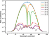 |
Fig. 1 Mean squared error of the network used as a predictor of all points in the range. At each iteration, the location of the point at the maximum location is added to the list of sampling points. |
2.1.3 Complex example
For a more complex test, we chose the chromospheric spectral line Ca II at 8542 Å. In this scenario, each profile can exhibit a wide range of shapes, including strong asymmetries and emission profiles. We used the synthetic data set of Stokes profiles and atmospheric models from Díaz Baso et al. (2022) to have a realistic and diverse representation of observed profiles (quiet-Sun, umbra, heating events, etc.). They were obtained as the reconstructed atmospheric models from nonlocal thermodynamic equilibrium (NLTE) inversions using the STiC code (de la Cruz Rodríguez et al. 2016, 2019) on high-resolution spectropolarimetric data acquired with CRISP at the SST (more details are available in Díaz Baso et al. 2021). This spectral line has a known asymmetry that arises from the presence of different isotopes (Leenaarts et al. 2014), and our method can use this feature to its advantage. However, we considered the spectral sampling symmetric to be able to easily compare it with the symmetric sampling suggested by de la Cruz Rodríguez et al. (2012), that is to say, we used half of the spectral line and the rest of the points are mirrored. The data set consists of 30000 Stokes profiles with 240 points in the wavelength range ±1.5 Å and an equidistant sampling of 12.5 mÅ, all synthesized with an observing angle μ = 1. For a consistent comparison with the former sampling, we assumed the same conditions: a Gaussian spectral filter transmission characterized by a full width at half maximum (FWHM) of 100 mÅ, an additive photon noise with a standard deviation σ = 10−3 relative to the continuum intensity, and the same number of points.
Once we generated and convolved the Stokes profiles of the data set, we followed the same procedure as before: we iteratively added the list of points with the largest errors according to the network prediction. Figure 3 shows the comparison with the sampling suggested by de la Cruz Rodríguez et al. (2012) in five different profiles. This sampling scheme and other similar versions have been used in previous SST observations (Díaz Baso et al. 2019; Yadav et al. 2021). It comprises a fine grid of points in the core and a coarser grid in the wings that depends on the instrumental spectral FWHM at the wavelength of the line. It consists of points spaced 50 mÅ from one another when close to the core and spaced by 500 mÅ in the wings. From the comparison, it is encouraging to see that our method provides a similar result compared to a strategy that resulted from the analysis of the sensitivity of the line and its improvement over time.
Figure 4 shows the evolution of the average error in different iterations for Stokes I and Stokes V. As a result, the final sampling scheme tends to have more points at locations where the profiles show more variability, which are the knees (enhancement around ±0.2Å) and the core of the Stokes I profiles, as well as the locations of the lobes of Stokes V. A similar result is found in the linear polarization parameters Stokes Q and Stokes U. For Stokes I, we find a sampling scheme with an average distance of 70 mÅ near the core and over 450 mÅ near the wings. For Stokes V, the average distance is about 65 mÅ in the core with no point until at the edge at −1.5Å because there is practically no signal in that region. These are just results from the statistical analysis of the signals, but they already show the implications for the inference of physical quantities: observations focused on magnetic field analysis should prioritize a denser grid near the core, while those focused on thermodynamic properties would benefit from a larger coverage (Felipe & Esteban Pozuelo 2019).
Although we have shown here how to implement this solution for individual Stokes parameters, it is also possible to take all Stokes parameters into account at once in the same merit function and weigh them appropriately according to the desired requirements. If the predictor network is well trained (and the number of points is not too large), the location of the points also generally satisfies Nyquist’s theorem and does not include points closer than half of the FWHM. This is expected because the spectral information has been degraded, so each spectral point contains information about the surrounding points that the network can use to estimate the values of points close in wavelength. In fact, if the instrumental resolution is worse, the method automatically tends to increase the separation of the points.
We note that if our set of profiles includes large velocities, we will obtain a sampling scheme with a wavelength distance larger than the original spectral resolution of the instrument in order to capture the details of the core when it is shifted far from the rest wavelength. So the minimum distance in the sampling scheme depends on the spectral resolution of the instrument, the typical broadening of the spectral shape, and the expected Doppler velocities.
In summary, this strategy is very simple and only needs a preexisting data set with spectral examples of the line of interest. They can be generated from numerical simulations or from previous observations with an instrument with a better spectral resolution, such as slit spectrographs.
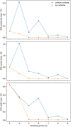 |
Fig. 2 Average error in the model parameters of the Gaussian fitting when using a uniform or an uncertainty-based sampling for a set of 10 000 profiles. |
2.2 Using model information
2.2.1 Description of the method
Although we see in Fig. 2 that the model parameters are recovered better with the new sampling scheme, we have no control over which solar atmospheric variables are being improved the most. However, if the physical model that generated that data set is also available, we can optimize the spectral sampling to improve the inference of a given constraint or model parameter. This is known as supervised selection since our target is now a product of the observed data. This problem becomes much more general and nonlinear than in the previous case, where we were only interested in keeping as much information as possible. As it will be too expensive to train a network for each combination of wavelength points, we can go back to the sequential strategy of the previous approach to speed up the search. The main difference is that now the function to minimize is the mse with respect to the model parameters. Let  represent our model parameters; each sample tk is a Q-dimensional vector that can contain as many parameters as we want to infer. Thus, the pseudocode, in this case, would be
If we examine both approaches, we see that while in the first one we tried to minimize the error at the worst wavelength, in this method we search for the new wavelength point that produces the best prediction. In this case, instead of training different neural networks for every configuration, the neural network has two inputs: one that is fixed (the sampling with the previous points) and a second input (xm, ym), which is one of the points from the pool. During the training, we randomly sample points from the pool to train a single neural network that can predict the output no matter what point of the pool is chosen. To test this method, we used the temperature stratification as a function of the optical depth scale at 5000 Å, hereafter log(τ500), associated with the intensity profiles of the same data set of the previous example. Figure 5 presents the root mse according to the number of iterations of the temperature stratification.
As a result, the new scheme again tends to place more points in the core than in the wings, similar to the previous case. While in the last example this result was purely due to the variability of the spectral line, in this case the reason (although related) is different. The two reasons are physically linked because the variability of the spectral line is due to the sensitivity of the line to changes in different regions of the solar atmosphere. To understand the correspondence in the physical parameters, we also calculated the error for a uniform sampling scheme. Figure 5 shows the error in the stratification of the temperature with 5 and 15 points in the full spectral range. From Fig. 5 we see that the error-guided method tends to decrease the error in the chromosphere (log(τ500) ≃ −4.5) for a low number of points as the average error in the chromosphere is larger than in any other location. After having a few points in the core, the following iterations add points in the wings, which help improve the estimation of the temperature of the lower atmosphere (log(τ500) ≃ −1.5). On the other hand, the uniform sampling is not guided by the uncertainty and follows a different behavior, improving first the lower atmosphere (for which we already had a good estimation) and later the rest of the atmosphere. This behavior occurs because the extension in wavelength where we have photospheric information is larger (a few angstroms in the wings) compared with the narrow wavelength region that samples a large range of heights in the chromosphere (see Fig. 4 in Kuridze et al. 2018). In the end, we see that the remaining error cannot decrease any further since it does not depend on the number of wavelength points but rather on the irreducible uncertainty resulting from the sensitivity of the line to the different heights in the solar atmosphere and the loss of information in the radiative transfer.
From this experiment, we show how a neural network can be used to indirectly estimate the average sensitivity of the profiles to the physical quantities of the model atmosphere, or in other words, the response functions (Ruiz Cobo & del Toro Iniesta 1992; Centeno et al. 2022). Given that the sensitivity of the observables to different parameters is also different, we also expect that optimizing the sampling to infer other quantities, such as the line-of-sight velocity or the magnetic field, will produce output schemes that will differ from the other cases. As stated in the previous section, given that we are optimizing a single merit function, we could combine as many physical quantities as we want or weigh them across the stratification, so the technique is optimized for a particular region of heights in the solar atmosphere.
We should recall that the training process of a neural network is non-deterministic and that the accuracy of the neural network is finite. This means we might arrive at a slightly different configuration after every run. This usually occurs with the last few points of the scheme, when the merit function has a very similar score everywhere. This problem could be alleviated with a network committee (ensemble), but in any case, the more points we add, the less essential it is to have an efficient design if we are already covering the whole area with many points. The use of the neural network as a surrogate function, in this case, allows us to overcome the very time-consuming process of inference in NLTE inversions. However, if a much simpler and deterministic model is available (e.g., the weak-field approximation), we recommend using such a model to eliminate the stochastic error inherent in the training process of the network, although simple but nonlinear models (e.g., a Milne-Eddington model) also have their own stochastic problems in finding the solution depending on the optimization method used and the parameter degeneracy.
We also note another caveat regarding the data set we have used. In our case, we synthesized the spectral lines assuming that the model atmosphere has not evolved during the time of the scan, and we only analyzed the impact of having different spectral resolution observations. A realistic study should include the scanning time effects when generating the sampling scheme, as shown by Felipe & Esteban Pozuelo (2019) and Schlichenmaier et al. (2023). This should help us better quantify the expected error in the inference when a specific temporal cadence is used.
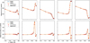 |
Fig. 3 Output sampling scheme as seen in five different profiles for Stokes I (upper panel) and Stokes V (lower panel) for the Ca II 8542 Å line. The sampling scheme suggested in de la Cruz Rodríguez et al. (2012) is also shown for comparison. The predicted profiles (output) are not visible because they are aligned behind synthetic profiles (target). |
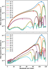 |
Fig. 4 Mean squared error of the predictor at every iteration for Stokes I and Stokes V for the Ca II line at 8542 Å. |
Future error-based spectral sampling
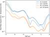 |
Fig. 5 Root mse of the network used as a predictor of the temperature stratification when there are 5 points (blue lines) and when there are 15 points (orange lines) in the whole wavelength range. The solid lines represent the error of the inferred sampling method, and the dashed lines are produced using the uniform sampling scheme. |
2.2.2 Model implications
In this last section, we want to show the implications of optimizing a wavelength scheme to the particularities of the chosen model. For this, we chose the weak-field approximation (WFA). In particular, we optimized our scheme to calculate the line-of-sight component of the magnetic field following the maximum likelihood estimation of BLOS in gauss (Martínez González et al. 2012):
 (1)
(1)
where the constant C0 = −4.67 × 10⁻¹³ [G−1 Å−1], λ0 in Å is the central wavelength of the line, and ɡeff is the effective Landé factor. Since we do not have to train any neural network, the optimization becomes a straightforward calculation, where the derivative of the profile is calculated by the finite differences, using the centered derivatives formula for non-equidistant grids (Sundqvist & Veronis 1970). Therefore, since Stokes V is the parameter that contains most of the information of BLOS, one would expect the optimization to sample this quantity like the result of Fig. 3. However, the estimation of the longitudinal field also depends on the derivative of Stokes I, and a poor sampling of Stokes I will also have a strong impact. In fact, the optimized output scheme has the location of the points extremely close to one another so that the truncation error in the derivative calculated with finite differences is smaller than the uncertainty introduced by Stokes V. If we provide the method with the exact value of the derivative, the method then tends to accommodate more points at the location of the Stokes V lobes. Given this result, optimizing the sampling to increase the accuracy to BLOS does not seem to be the smartest choice if we want to extract other information. A better idea would be to use the scheme in Fig. 3 and use the trained network to interpolate the Stokes I profile to a finer mesh, where we can compute the derivative. In Fig. 6 we show the effect on the derivative of the Stokes I profile for a given example using various methods. In general, the derivative of the profile estimated with the neural network has a higher accuracy, although other spline-based interpolation methods could be used when there are a large number of points. For a low number of points, the neural network performs much better. In terms of magnetic fields, for the case of a scheme with 21 points and a noise level of 10−3 in units of the continuum, the root mse for this database is on the order of 800 G for the uniform case, 200 G when using the sampling guided by the neural network outlined in Sect. 2.1, 60 G when the same neural network is used for predicting the full profile, and 30 G for the case of a very fine grid in Stokes I and V.
Therefore, we conclude that (for FPI observations) using models that fit the Stokes profiles directly (such as a Milne-Eddington model) could be more accurate than models, such as the WFA, that also depend on the derivatives of the Stokes profiles. Recently, a modified Milne-Eddington approximation has been developed to allow much better modeling of chromospheric lines (Dorantes-Monteagudo et al. 2022) if speed is needed. On the other hand, if precision is required, we recommend NLTE modeling for the inference.
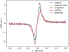 |
Fig. 6 Derivative of Stokes I with respect to the wavelengths for the Ca II line at 8542 Å using the original synthetic profile, the optimized sampling found in Sect. 2.1, a uniform sampling, and the prediction of the neural network for the full profile. |
2.3 Sampling parameterization
Finally, although we have shown a method flexible enough to find the points in wavelength that retain the most information and improve our parameter inference, in some cases we may want the distances of the points to obey other constraints, such as being multiples of a uniform grid to perform computationally efficient fast Fourier transforms, for instrumental reasons or just because the interface of some spectral inversion codes requires it. In this case, one can parameterize the sampling (for example, by defining the inner distance, the distance factor for outer points, and the number of inner points) and train our predictor for several cases. Later we can evaluate the different configurations (in this three-dimensional space) and find which configuration is optimal. An example of this idea is shown in Fig. 7, where we present the optimal configuration for a uniform sampling (top row) and another in which we allow the outer points to be farther apart (bottom row). As a result, we find a 13-point scheme (steps of 95 mÅ, 7 inner points, an outer factor of 5) whose performance is better than a completely uniform scheme with 19 points (steps of 120 mÅ). Both are the best configurations for their respective number of points to have a fair comparison. Using this strategy, we can find schemes with fewer points that still obey our constraints.
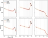 |
Fig. 7 Optimal sampling where all points have the same distance (upper row) and where outer points are spaced multiple times wider than the inner points (bottom row). |
3 Conclusions
In this study, we have explored, developed, and validated a machine-learning technique to design efficient sampling schemes for accurate parameter estimation using filtergraph instruments. The problem of finding an optimal wavelength configuration has been framed as a feature selection problem. Only those points (features) that contain relevant information and improve the model prediction are chosen to be in the sampling scheme. We have implemented two approaches: if only the spectra are available (unsupervised selection) or if the model information is used to improve the inference of the physical quantities (supervised selection). We have implemented a sequential approach where a neural network is used to predict the target from the information at a few points, and in that way we can measure the importance of different wavelength points. We validated the performance of the new sampling schemes compared to a uniformly spaced sampling by showing the lower errors in the reconstructions of the model parameters. This approach is particularly efficient for a small number of points, which is crucial when observers are interested in highly dynamic events and a good temporal cadence is needed. Also, if we expect large Doppler velocities or the spectral resolution of our instrument is poor, this method will adapt the scheme accordingly. Both the method description and the code implementation are publicly available.
From the experiments that used the Ca II 8542 Å line, we were able to extract some results that can be used as practical recommendations for future observations. For example, the resulting wavelength scheme naturally places (almost a factor of 4) more points in the core (±0.5 Å) than in the wings, consistent with the sensitivity of the spectral line in each wavelength range. In addition, observations focused on magnetic field analysis should prioritize a denser grid near the core where the polarization signals are present, while those focused on thermodynamic properties would benefit from a larger coverage (Felipe & Esteban Pozuelo 2019). In conclusion, the selection of the wavelength points depends on the goal of the observations.
Regarding the methodology, it is difficult to ensure that this technique provides a global solution to the problem (if there is one), but it provides an efficient scheme, much better than a uniform strategy. Therefore, this method can be helpful when designing new instrumentation or when designing the wavelength configuration in observing proposals for a specific target. This trained network can also be used after the observations to estimate the complete profile from the points obtained, thus helping the inference process when using NLTE inversion codes (de la Cruz Rodríguez et al. 2019) or obtaining a more accurate estimation of the derivative of Stokes I when using the WFA to infer the magnetic field.
Finally, there are several ways in which we could improve the current implementation, for example by solving the full problem at once because the neural network makes the problem differentiable. Using gradient-based techniques, we could find the solution by applying a regularization term (e.g., ℓ0 norm) that penalizes a large number of points. We tried this option, but it was not possible to converge in most cases as the full problem is much more degenerated (i.e., it has the location of all wavelength points as free parameters at the same time) than when using a sequential method. Regarding the ultimate goal of the technique, this procedure is so flexible that it could also be generalized to include the exposure time at each wavelength. By doing so, the merit function would be sensitive to the signal-to-noise ratio at each point, and we could obtain a better design by taking the trade-off between the weak polarization signals and the evolution time of the Sun into account. From the neural network perspective, there are also ways to speed up the training and decrease the stochasticity of the process by using networks that better exploit the relation between different regions of the spectrum (such as transformer or graph networks) or by reformulating the problem with reinforcement learning to mitigate the nested behavior of sequential approaches. In summary, we plan to continue investigating this strategy and provide optimal wavelength schemes for different spectral lines, instrumentation, and solar targets in future work.
Acknowledgements
We would like to thank the anonymous referee for their comments and suggestions. C.J.D.B. thanks Ignasi J. Soler Poquet, João M. da Silva Santos and Henrik Eklund for their comments. This research is supported by the Research Council of Norway, project number 325491 and through its Centers of Excellence scheme, project number 262622. This project has received funding from the European Research Council (ERC) under the European Union’s Horizon 2020 research and innovation program (SUNMAG, grant agreement 759548). The Institute for Solar Physics is supported by a grant for research infrastructures of national importance from the Swedish Research Council (registration number 2021-00169). We acknowledge the community effort devoted to the development of the following open-source packages that were used in this work: NumPy (href://numpy.org), Matplotlib (href://matplotlib.org), SciPy (href://scipy.org), Astropy (href://astropy.org) and PyTorch (href://pytorch.org). This research has made use of NASA’s Astrophysics Data System Bibliographic Services.
References
- Anusha, L. S., van Noort, M., & Cameron, R. H. 2021, ApJ, 911, 71 [NASA ADS] [CrossRef] [Google Scholar]
- Cavallini, F. 2006, Sol. Phys., 236, 415 [NASA ADS] [CrossRef] [Google Scholar]
- Centeno, R., Flyer, N., Mukherjee, L., et al. 2022, ApJ, 925, 176 [NASA ADS] [CrossRef] [Google Scholar]
- de la Cruz Rodríguez, J. & van Noort, M. 2017, Space Sci. Rev., 210, 109 [CrossRef] [Google Scholar]
- de la Cruz Rodríguez, J., Socas-Navarro, H., Carlsson, M., & Leenaarts, J. 2012, A&A, 543, A34 [Google Scholar]
- de la Cruz Rodríguez, J., Leenaarts, J., & Asensio Ramos, A. 2016, ApJ, 830, L30 [Google Scholar]
- de la Cruz Rodríguez, J., Leenaarts, J., Danilovic, S., & Uitenbroek, H. 2019, A&A, 623, A74 [Google Scholar]
- Díaz Baso, C. J., Martínez González, M. J., Asensio Ramos, A., & de la Cruz Rodríguez, J. 2019, A&A, 623, A178 [NASA ADS] [CrossRef] [EDP Sciences] [Google Scholar]
- Díaz Baso, C. J., de la Cruz Rodríguez, J., & Leenaarts, J. 2021, A&A, 647, A188 [NASA ADS] [CrossRef] [EDP Sciences] [Google Scholar]
- Díaz Baso, C. J., Asensio Ramos, A., & de la Cruz Rodríguez, J. 2022, A&A, 659, A165 [NASA ADS] [CrossRef] [EDP Sciences] [Google Scholar]
- Dorantes-Monteagudo, A. J., Siu-Tapia, A. L., Quintero-Noda, C., & Orozco Suárez, D. 2022, A&A, 659, A156 [NASA ADS] [CrossRef] [EDP Sciences] [Google Scholar]
- Felipe, T., & Esteban Pozuelo, S. 2019, A&A, 632, A75 [NASA ADS] [CrossRef] [EDP Sciences] [Google Scholar]
- Felipe, T., Socas-Navarro, H., & Przybylski, D. 2018, A&A, 614, A73 [NASA ADS] [CrossRef] [EDP Sciences] [Google Scholar]
- Gudiksen, B. V., Carlsson, M., Hansteen, V. H., et al. 2011, A&A, 531, A154 [NASA ADS] [CrossRef] [EDP Sciences] [Google Scholar]
- Guyon, I., & Elisseeff, A. 2003, J. Mach. Learn. Res., 3, 3 [Google Scholar]
- He, K., Zhang, X., Ren, S., & Sun, J. 2015, arXiv e-prints [arXiv:1512.03385] [Google Scholar]
- Iglesias, F. A., & Feller, A. 2019, Opt. Eng., 58, 082417 [Google Scholar]
- Kingma, D. P., & Ba, J. 2014, arXiv e-prints [arXiv:1412.6980] [Google Scholar]
- Kuridze, D., Henriques, V. M. J., Mathioudakis, M., et al. 2018, ApJ, 860, 10 [Google Scholar]
- Leenaarts, J., & Carlsson, M. 2009, ASP Conf. Ser., 415, 87 [Google Scholar]
- Leenaarts, J., de la Cruz Rodríguez, J., Kochukhov, O., & Carlsson, M. 2014, ApJ, 784, L17 [NASA ADS] [CrossRef] [Google Scholar]
- Lemen, J. R., Title, A. M., Akin, D. J., et al. 2012, Sol. Phys., 275, 17 [Google Scholar]
- Lewis, D. D., & Catlett, J. 1994, in Machine Learning Proceedings 1994, eds. W. W. Cohen, & H. Hirsh (San Francisco (CA): Morgan Kaufmann), 148 [CrossRef] [Google Scholar]
- Li, J., Cheng, K., Wang, S., et al. 2017, ACM Comput. Surv., 50, 50 [Google Scholar]
- Lim, D., Moon, Y.-J., Park, E., & Lee, J.-Y. 2021, ApJ, 915, L31 [NASA ADS] [CrossRef] [Google Scholar]
- Magdaleno, E., Rodríguez Valido, M., Hernández, D., et al. 2022, Sensors (Basel), 22, 22 [Google Scholar]
- Martínez González, M. J., Manso Sainz, R., Asensio Ramos, A., & Belluzzi, L. 2012, MNRAS, 419, 153 [CrossRef] [Google Scholar]
- Milić, I., & van Noort, M. 2018, A&A, 617, A24 [Google Scholar]
- Nóbrega-Siverio, D., Martínez-Sykora, J., Moreno-Insertis, F., & Carlsson, M. 2020, A&A, 638, A79 [EDP Sciences] [Google Scholar]
- Osborne, C. M. J., & Milić, I. 2021, ApJ, 917, 14 [NASA ADS] [CrossRef] [Google Scholar]
- Panos, B., & Kleint, L. 2021, ApJ, 915, 77 [NASA ADS] [CrossRef] [Google Scholar]
- Panos, B., Kleint, L., & Voloshynovskiy, S. 2021, ApJ, 912, 121 [NASA ADS] [CrossRef] [Google Scholar]
- Pedregosa, F., Varoquaux, G., Gramfort, A., et al. 2011, J. MaCh. Learn. Res., 12, 12 [NASA ADS] [Google Scholar]
- Pesnell, W. D., Thompson, B. J., & Chamberlin, P. C. 2012, Sol. Phys., 275, 3 [Google Scholar]
- Przybylski, D., Cameron, R., Solanki, S. K., et al. 2022, A&A, 664, A91 [NASA ADS] [CrossRef] [EDP Sciences] [Google Scholar]
- Pudil, P., Novovicová, J., & Kittler, J. 1994, Pattern Recognit. Lett., 15, 1119 [Google Scholar]
- Puschmann, K. G., Denker, C., Kneer, F., et al. 2012, Astron. NaChr., 333, 880 [NASA ADS] [CrossRef] [Google Scholar]
- Quintero Noda, C., Schlichenmaier, R., Bellot Rubio, L. R., et al. 2022, A&A, 666, A21 [NASA ADS] [CrossRef] [EDP Sciences] [Google Scholar]
- Raschka, S. 2018, J. Open SourCe Softw., 3, 3 [Google Scholar]
- Rimmele, T. R., Warner, M., Keil, S. L., et al. 2020, Sol. Phys., 295, 172 [Google Scholar]
- Ruiz Cobo, B., & del Toro Iniesta, J. C. 1992, ApJ, 398, 375 [Google Scholar]
- Salvatelli, V., dos Santos, L. F. G., Bose, S., et al. 2022, ApJ, 937, 100 [NASA ADS] [CrossRef] [Google Scholar]
- Scharmer, G. 2017, in SOLARNET IV: The PhysiCs of the Sun from the Interior to the Outer Atmosphere, 85 [Google Scholar]
- Scharmer, G. B., Bjelksjo, K., Korhonen, T. K., Lindberg, B., & Petterson, B. 2003, in ProC. SPIE, 4853, 341 [NASA ADS] [CrossRef] [Google Scholar]
- Scharmer, G. B., Narayan, G., Hillberg, T., et al. 2008, ApJ, 689, L69 [Google Scholar]
- Schlichenmaier, R., Pitters, D., Borrero, J. M., & Schubert, M. 2023, A&A, 669, A78 [NASA ADS] [CrossRef] [EDP Sciences] [Google Scholar]
- Schmidt, W., Bell, A., HalbgewaChs, C., et al. 2014, SPIE Conf. Ser., 9147, 91470E [NASA ADS] [Google Scholar]
- Settles, B. 2012, Synthesis LeCtures on ArtifiCial IntelligenCe and MaChine Learning, 6, 6 [CrossRef] [Google Scholar]
- Socas-Navarro, H., de la Cruz Rodríguez, J., Asensio Ramos, A., Trujillo Bueno, J., & Ruiz Cobo, B. 2015, A&A, 577, A7 [NASA ADS] [CrossRef] [EDP Sciences] [Google Scholar]
- Solanki, S. K., del Toro Iniesta, J. C., Woch, J., et al. 2020, A&A, 642, A11 [NASA ADS] [CrossRef] [EDP Sciences] [Google Scholar]
- Štěpán, J., & Trujillo Bueno, J. 2013, A&A, 557, A143 [NASA ADS] [CrossRef] [EDP Sciences] [Google Scholar]
- Sundqvist, H., & Veronis, G. 1970, Tellus, 22, 22 [Google Scholar]
- Uitenbroek, H. 2001, ApJ, 557, 389 [Google Scholar]
- Vögler, A., Shelyag, S., Schüssler, M., et al. 2005, A&A, 429, 335 [Google Scholar]
- Whitney, A. 1971, IEEE Trans. Comput., C-20, C-20 [Google Scholar]
- Yadav, R., Díaz Baso, C. J., de la Cruz Rodríguez, J., Calvo, F., & Morosin, R. 2021, A&A, 649, A106 [NASA ADS] [CrossRef] [EDP Sciences] [Google Scholar]
Our implementation can be found in the following repository: https://github.com/cdiazbas/active_sampling
All Tables
All Figures
|
Fig. 1 Mean squared error of the network used as a predictor of all points in the range. At each iteration, the location of the point at the maximum location is added to the list of sampling points. |
| In the text | |
|
Fig. 2 Average error in the model parameters of the Gaussian fitting when using a uniform or an uncertainty-based sampling for a set of 10 000 profiles. |
| In the text | |
|
Fig. 3 Output sampling scheme as seen in five different profiles for Stokes I (upper panel) and Stokes V (lower panel) for the Ca II 8542 Å line. The sampling scheme suggested in de la Cruz Rodríguez et al. (2012) is also shown for comparison. The predicted profiles (output) are not visible because they are aligned behind synthetic profiles (target). |
| In the text | |
|
Fig. 4 Mean squared error of the predictor at every iteration for Stokes I and Stokes V for the Ca II line at 8542 Å. |
| In the text | |
|
Fig. 5 Root mse of the network used as a predictor of the temperature stratification when there are 5 points (blue lines) and when there are 15 points (orange lines) in the whole wavelength range. The solid lines represent the error of the inferred sampling method, and the dashed lines are produced using the uniform sampling scheme. |
| In the text | |
|
Fig. 6 Derivative of Stokes I with respect to the wavelengths for the Ca II line at 8542 Å using the original synthetic profile, the optimized sampling found in Sect. 2.1, a uniform sampling, and the prediction of the neural network for the full profile. |
| In the text | |
|
Fig. 7 Optimal sampling where all points have the same distance (upper row) and where outer points are spaced multiple times wider than the inner points (bottom row). |
| In the text | |
Current usage metrics show cumulative count of Article Views (full-text article views including HTML views, PDF and ePub downloads, according to the available data) and Abstracts Views on Vision4Press platform.
Data correspond to usage on the plateform after 2015. The current usage metrics is available 48-96 hours after online publication and is updated daily on week days.
Initial download of the metrics may take a while.