| Issue |
A&A
Volume 673, May 2023
|
|
|---|---|---|
| Article Number | A80 | |
| Number of page(s) | 13 | |
| Section | Stellar structure and evolution | |
| DOI | https://doi.org/10.1051/0004-6361/202245696 | |
| Published online | 10 May 2023 | |
Empirical determination of the lithium 6707.856 Å wavelength in young stars⋆
1
European Southern Observatory, Karl-Schwarzschild-Strasse 2, 85748 Garching bei München, Germany
e-mail: jcampbel@eso.org
2
SUPA, School of Science and Engineering, University of Dundee, Nethergate, Dundee DD1 4HN, UK
3
INAF – Osservatorio Astrofisico di Catania, Via S. Sofia, 78, 95123 Catania, Italy
4
Hamburg Observatory, Gojenbergsweg 11, 21029 Hamburg, Germany
5
INAF – Osservatorio Astronomico di Roma: Monte Porzio Catone, Lazio, Italy
6
Instituto de Física y Astronomía, Universidad de Valparaíso, Gran Bretaña, 1111 Valparaíso, Chile
7
University Observatory, Faculty of Physics, Ludwig-Maximilians-Universität München, Scheinerstr. 1, 81679 Munich, Germany
8
Excellence Cluster ‘Origins’, Boltzmannstr. 2, 85748 Garching, Germany
9
Konkoly Observatory, Research Centre for Astronomy and Earth Sciences, Eötvös Loránd Research Network (ELKH), Konkoly-Thege Miklós út 15-17, 1121 Budapest, Hungary
10
CSFK, MTA Centre of Excellence, Konkoly-Thege Miklós út 15-17, 1121 Budapest, Hungary
11
ELTE Eötvös Loránd University, Institute of Physics, Pázmány Péter sétány 1/A, 1117 Budapest, Hungary
12
Purple Mountain Observatory, Chinese Academy of Sciences, 10 Yuanhua Road, Nanjing 210023, PR China
13
INAF-Osservatorio Astrofisico di Arcetri, L.go E. Fermi 5, 50125 Firenze, Italy
14
Instituto de Astrofísica e Ciências do Espaço, Universidade do Porto, CAUP, Rua das Estrelas, 4150-762 Porto, Portugal
15
Departamento de Física e Astronomia, Faculdade de Ciências, Universidade do Porto, rua do Campo Alegre 687, 4169-007 Porto, Portugal
16
ASI, Italian Space Agency, Via del Politecnico snc, 00133 Rome, Italy
17
Max Planck Institute for Astronomy, Königstuhl 17, 69117 Heidelberg, Germany
18
Instituto de Astronom ia, Universidad Nacional Autónoma de México, Carr. Tijuana-Ensenada km107, C.I.C.E.S.E., 22860 Ensenada, B.C., Mexico
19
INAF – Osservatorio Astronomico di Padova, Vicolo dell’osservatorio 5, 35122 Padova, Italy
20
Department of Physics & Astronomy, Amherst College, C025 Science Center 25 East Drive, Amherst, MA 01002, USA
21
SETI Institute, 339 Bernardo Ave, Suite 200, Mountain View, CA 94043, USA
Received:
15
December
2022
Accepted:
7
March
2023
Absorption features in stellar atmospheres are often used to calibrate photocentric velocities for the kinematic analysis of further spectral lines. The Li feature at ∼6708 Å is commonly used, especially in the case of young stellar objects, for which it is one of the strongest absorption lines. However, this complex line comprises two isotope fine-structure doublets. We empirically measured the wavelength of this Li feature in a sample of young stars from the PENELLOPE/VLT programme (using X-shooter, UVES, and ESPRESSO data) as well as HARPS data. For 51 targets, we fit 314 individual spectra using the STAR-MELT package, resulting in 241 accurately fitted Li features given the automated goodness-of-fit threshold. We find the mean air wavelength to be 6707.856 Å, with a standard error of 0.002 Å (0.09 km s−1), and a weighted standard deviation of 0.026 Å (1.16 km s−1). The observed spread in measured positions spans 0.145 Å, or 6.5 km s−1, which is higher by up to a factor of six than the typically reported velocity errors for high-resolution studies. We also find a correlation between the effective temperature of the star and the wavelength of the central absorption. We discuss that exclusively using this Li feature as a reference for photocentric velocity in young stars might introduce a systematic positive offset in wavelength to measurements of further spectral lines. If outflow tracing forbidden lines, such as [O I] 6300 Å, is more blueshifted than previously thought, this then favours a disc wind as the origin for this emission in young stars.
Key words: stars: atmospheres / stars: pre-main sequence / stars: variables: T Tauri, Herbig Ae/Be / ISM: abundances
© The Authors 2023
 Open Access article, published by EDP Sciences, under the terms of the Creative Commons Attribution License (https://creativecommons.org/licenses/by/4.0), which permits unrestricted use, distribution, and reproduction in any medium, provided the original work is properly cited.
This article is published in open access under the Subscribe to Open model. Subscribe to A&A to support open access publication.
1. Introduction
Lithium is a benchmark element in stellar astrophysics and causes prominent photospheric features in optical spectra of young stellar objects (YSOs). In particular, the Li I ∼6708 Å feature is often (one of) the strongest photospheric absorption lines. The lines from other metals are more prone to line-dependent veiling. This Li feature is used to age star clusters from the lithium depletion boundary (e.g., Messina et al. 2016; Gutiérrez Albarrán et al. 2020; Binks et al. 2022) and to identify young stars (e.g., Walter et al. 1994; Montes et al. 2001; Bayo et al. 2011; Jeffries et al. 2017). Furthermore, the position of the Li feature is fundamentally important as a reference for establishing the photocentric velocity, in particular, for kinematic studies of YSO emission line properties.
The absorption feature consists of multiple fine-structure1 transitions of both 7Li and 6Li (Kurucz 1995; Morton 2003). The typical abundance of the more fragile 6Li has been found to be < 10% for a range of stellar types (e.g., Fields & Olive 2022, and references therein). The complexity of this absorption feature is due to the two spin-orbit electronic transitions from the 2P to the 2S level of 7Li, alongside any lesser contribution from the same transitions of 6Li. Table 1 shows the air wavelengths of these components (we use air wavelengths throughout). From the L-S coupling and the gyromagnetic ratios, each doublet is in a 2:1 resonance, and the D2 lines are the stronger of the pairs. Additionally, these lines are adjacent to spectral lines of Fe I, Si I, V I, and Cr I (see Table 2 in Franciosini et al. 2022a, and Fig. A.1), which commonly appear to be blended with the Li feature. From this simple consideration, it is clear that the centroid of this feature should not have a constant position in YSO spectra.
Line centres and oscillator strengths of the components of the Li Iλ6708 Å line (Morton 2003).
Previous studies that took the Li feature as reference for photocentric calibration of YSO spectra have used positions from 6707.800 Å to 6707.876 Å (Edwards et al. 1987; Cabrit et al. 1990; Natta et al. 2014; Pascucci et al. 2015; Simon et al. 2016; Nisini et al. 2018). The reason was that further spectral features, such as outflow tracing forbidden lines, can be kinematically measured with respect to the stellar photospheric rest frame. A commonly used emission line is [O I] 6300 Å, which can readily be decomposed into a high- (v ≳ 30–50 km s−1) and low-velocity component (HVC and LVC, respectively). The LVC is further comprised of a narrow (NC) and broad component (BC) (Banzatti et al. 2019; Pascucci et al. 2022). Small blueshifts of the LVC centroid by a few km s−1 were noted for instance by Hartigan et al. (1995) and Rigliaco et al. (2013), who suggested that this is a clear sign of unbound gas flowing outwards from the disc. Banzatti et al. (2019) found that for low LVC blueshifts from discs with an inner cavity, the blueshift reduces as the inner dust from the disc clears and emission originates from farther out in the disc. However, surveys of the [O I] 6300 Å line in YSOs showed that this line is centred at the photocentric velocity for almost half of the samples (Simon et al. 2016; Nisini et al., in prep.). Another possible source of the LVC is gas that is bound to the star or inner disc. It is still difficult to disentangle the possible sources of the forbidden line emission, regardless of whether it is photoevaporative, magnetohydrodynamic (MHD), or non-thermal outflows (Nemer et al. 2020), especially for the NC of the LVC. Weber et al. (2020) showed that photoevaporation reproduces most of the observed NCs, but not the BCs or the HVCs, whereas MHD winds are able to reproduce all components, but produce Keplerian double peaks that disagree with observations. It is therefore important to determine whether the LVC is centred at the photocentric rest velocity or is shifted. Models from Ercolano & Owen (2016) suggested that even the slightest blueshift is a tell-tale sign of a disc wind. In massive environments, external photoevaporation could lead to shifts of less than ∼2 km s−1 (Ballabio et al. 2023).
Since these [O I] 6300 Å and other forbidden line LVC velocities are measured within a few km s−1 of the stellar velocity, it is clear that an accurate determination of this velocity for YSOs is critical for a subsequent kinematic analysis. We report a systematic empirical study of the position of the Li ∼6708 Å feature based on a sample of YSOs using mid- to high-resolution spectrographs. This will allow future studies of forbidden line kinematics to avoid potential systematic offsets that were unforeseen until now.
2. YSO sample and observations
The YSO spectra used in this work were obtained using the ESO instruments Echelle SPectrograph for Rocky Exoplanets and Stable Spectroscopic Observations (ESPRESSO), Ultraviolet and Visual Echelle Spectrograph (UVES), and X-shooter (on the ESO Very Large Telescope, VLT), and High Accuracy Radial velocity Planet Searcher (HARPS, on the ESO 3.6 m). VLT data are from the public PENELLOPE survey (Manara et al. 2021). This survey was contemporaneous to the HST/ULLYSES2 program3, during which 82 young stars were observed by the HST. Spectroscopic data reduction was carried out using the ESO Reflex workflow v2.8.5 (Freudling et al. 2013). Telluric correction was also performed using MOLECFIT (Smette et al. 2015; Kausch et al. 2015)4.
Here, we include repeated VLT observations of 41 stars from the ULLYSES sample that are from the Orion OB1 and σ Orionis associations (as presented in Manara et al. 2021) as well as Cha I, η Cha, and Lupus. This sample covers YSOs with spectral types K2 through M5 and a wide range of disc ages (∼1–10 Myr) and evolutionary stages.
We also include ten YSOs with repeated HARPS observations from Pr. ID. 105.207T (P.I. Campbell-White), acquired to investigate the temporal spectral evolution of YSOs of different mass ranges. This sub-sample includes targets at earlier spectral type (G5 through M1) than the PENELLOPE sample. The HARPS data for four targets also have more repeated observations of each star (from 8 to 15; see Appendix C). The 1D spectra were used, with data reduction carried out using the standard ESO pipeline, and no further corrections were applied. There is no significant influence from telluric lines around the position of the Li 6708 Å line.
No photospheric corrections were applied to any of the data used in this work. Although this might remove blends from around the Li absorption (for a Li-poor template or a synthetic spectrum), we did not consider this correction because the aim of this investigation is to understand the measured position of the Li absorption. Moreover, as the centroid of the Li feature is normally measured in the observed spectra without subtracting a photospheric template, we have purposely made our measurements including the effect of the line blends.
3. Method
From the observations of the 51 targets we outlined, 314 YSO spectra were fitted with STAR-MELT: 92 from HARPS, 72 from UVES, 61 from X-shooter, and 88 from ESPRESSO. Barycentric correction was applied to the UVES and X-shooter air wavelength frames. ESPRESSO and HARPS already use this standard. Stellar photocentric radial velocities (RVs) were calculated for each individual observation around the wavelength range of 6000–6250 Å, using the standard RV templates of the STAR-MELT package (Campbell-White et al. 2021). This ensured that the Li centroid was measured with respect to any intrinsic stellar RV variations. We selected this range to include further prominent photospheric absorption lines (as in e.g., Fang et al. 2018) close to but not including the Li absorption line itself to avoid wavelength-dependent RV variations (e.g., Martín et al. 2006).
An arbitrary reference wavelength of 6708.0 Å was then used to measure the positions of the Li absorption lines, which were fitted with a single Gaussian plus a linear component (the latter to fit the local continuum and help account for asymmetries). A velocity range of 150 km s−1 was used for each fit. This adequately covered the full absorption plus continuum of each Li observation. The centre of the Gaussian component was obtained for each observation, with associated standard errors from the least-squares optimisation fitting. The shift with respect to the reference wavelength thus gives the centroid or photocenter of the Li absorption line for each observation.
The automated fitting and goodness-of-fit restrictions using STAR-MELT (see Appendix A) resulted in 241 accurately fitted individual observations across the YSO spectra. This is more 75% of the initial sample. The reasons for the subset of larger errors primarily include data with a lower signal-to-noise ratio (S/N), binaries (e.g., CVSO104; Frasca et al. 2021), and non-detections of Li from the HARPS sample, also due to low S/N, likely continuum veiling, and/or stellar age. Li was detected in all YSOs from the PENELLOPE sample.
We note that in the recent work of Franciosini et al. (2022a) on Li abundances from the Gaia/ESO survey multiple Gaussian component fits were used for the UVES spectra to model the two components of the Li doublet (for the FGK stars), as well as adjacent Fe and Si blends. Whilst this is important for measuring equivalent widths (EWs), we find that for our YSO sample from UVES (and even the higher-resolution ESPRESSO and HARPS data), the feature centre is well fitted by the single Gaussian plus linear component in each instance. Increasing the number of components in an attempt to more accurately model the doublet does not improve the calculated χ2 goodness-of-fit, nor does it shift the overall centre of the fit by more than the typical measurement errors we report (≲1 km s−1; see Fig. A.2). Since we are interested in the position of the feature centroid (as it is measured for photocentric RV calibrations), the fitting procedure we used remains accurate in this sense.
4. Analysis and discussion
Figure 1 shows a box plot of the measured Li positions across all data, split by instrument. The overall mean wavelength of the Li absorption line is 6707.856 Å, with a standard error of 0.002 Å (0.09 km s−1) and a weighted standard deviation of 0.026 Å (1.16 km s−1). This observed spread in measured values spans 0.145 Å, or 6.5 km s−1. The grey shaded area in Fig. 1 indicates the range of Li wavelengths that were used to measure stellar RVs from a sample of previous studies (Natta et al. 2014; Pascucci et al. 2015; Simon et al. 2016; Nisini et al. 2018).
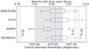 |
Fig. 1. Box plot of the resulting central wavelength position from fitting all of the PENELLOPE VLT (ESPRESSO, UVES, X-shooter) and the further HARPS YSO spectra. The boxes extend from the lower to upper quartile values of the data, with a green line at the median. The whiskers extend to 1.5 times the box range. Outliers are indicated by circles. The mean central wavelength position is marked by the dashed magenta line. Positions of the 7Li D1, D2, and 6Li D2 lines are indicated by the dashed and dash-dotted black lines. The grey shaded area indicates the range of values of the Li I line centres that were used as reference for the RV calculations in previous works. |
4.1. Wavelength of Li absorption
The Li absorption feature mean wavelength we observe agrees well with previous studies that measured this line (e.g., 6707.851 ± 0.007 Å from observations of a carbon star; Wallerstein 1977). Figure 1 shows that the median values obtained from the UVES and X-shooter data are also close to this overall value. The median values of ESPRESSO and HARPS data, however, lie either side of the overall sample mean. Since these instruments have similar resolving power, this is probably an observed effect from the sub-samples. Any potential instrumental influences were carefully checked. In the following subsection, we discuss the most prominent correlation with respect to the observed spread of Li centroids. To preface this, we first briefly discuss further potential sources of the Li shifts.
For YSOs, accretion-related activity causes wavelength-dependent continuum veiling. Corrections for veiling have been made to the observed Li feature in T Tauri stars (e.g., Basri et al. 1991; Biazzo et al. 2017), and determination of the photospheric abundances using NLTE effects in YSOs indicates that their lithium abundance is usually close to cosmic (Magazzu et al. 1992; Martin et al. 1994). It is likely that the Li6/Li7 isotopic ratio of YSOs is also cosmic. Recently, Wang et al. (2022) used 3D NLTE radiative transfer methods to model ESPRESSO spectra of metal poor stars, finding extremely low isotopic Li6/Li7 ratios. This has not yet been carried out for YSOs, however. We hence assume that differences in the Li isotopic ratio are negligible and do not significantly influence the observed Li feature position in our sample of young stars.
Slight differences in the lithium abundance across different stars may, however, affect the observed position by determining how influential the adjacent Fe I line blend is on the overall shape and centre of the feature. If the Fe I is stronger, then we would expect a higher blueshift of the photocentre of the whole feature. Metallicity of the stars would also contribute significantly (Franciosini et al. 2022a). For cool, active stars, the fractional coverage of star spots also affects the measured Li abundances (Franciosini et al. 2022b), which is further discussed in this section.
We find no clear correlation between the EW of the Li feature and its central wavelength, suggesting that the intensity of the Li I plays a minor role in its observed position, at least in the range of abundances covered by our sample. Although the more strongly blended lines may have larger EWs, as the Li EW increases with the elemental abundance, no potential trend is apparent here. Our results are similar to those from Biazzo et al. (2017), who reported EWs and Teff that agreed well with NLTE curves of growth, but the lowest Teff stars do not exclusively show the smallest EWs. This suggests that our sample has higher abundances overall.
As outlined, another potential contributor to the spread of Li position values is the active nature of YSOs. Even in the case of non-accreting objects, the strong magnetic activity gives rise to cool photospheric star spots that can distort the absorption line profiles and change the centroid (e.g., Biazzo et al. 2009; Lanza et al. 2018). Furthermore, accretion-related activity can affect the measured RVs (Sicilia-Aguilar et al. 2015; Alcalá et al. 2017; Campbell-White et al. 2021). Continuum-veiling differences might affect the measured abundances and EWs of the Li and the adjacent lines. A ROTFIT analysis of the PENELLOPE data shows that the veiling changes daily (Manara et al. 2021). Recent work on RU Lup by Stock et al. (2022) showed significant veiling differences for this K7 star across 12 nights. We may also have line-dependent veiling such that the Li remains in absorption, but the blended Fe or Si lines could have an emission component, which would alter the measured centroid of the absorption line. From our results, we detect no significant correlation with the veiling measured at 650 nm and the central Li position (see Fig. B.2). Therefore, if veiling does have an influence, it appears to not to affect the position of the Li line systematically. We find no significant correlation between the log g of the YSOs and the central position of the Li line either (Fig. B.3).
4.2. Effective temperature correlation
Figure 2 shows the measured central position of the Li feature vs. the effective temperature (Teff) of the star. Points are coloured by instrument, and the histograms show the two distributions. In the top panel, the corresponding measured Li wavelength is also shown, along with the positions of the 7Li D1 and D2 and the 6Li D1 components. The mean value is marked by the magenta line.
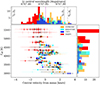 |
Fig. 2. Teff vs. velocity difference from the mean measured Li centroid position. Stars indicate the mean measured position for each target. The shaded boxes show the 1σ spread of measurements. Circles indicate that Teff measurements are from ROFIT/PENELLOPE spectra, and triangles are taken from the TESS input catalogue. We note an anti-correlation (r = −0.58) between Teff and mean position: lower Teff stars show more redshifted central values. The total velocity error bars arise from adding the standard errors of the RV and Gaussian centre measurements in quadrature. Faded markers and error bars are measurements with total velocity errors 0.75 km s−1. The mean measured Li centroid and positions of the D line components are indicated in the top histogram. |
Teff values for the PENELLOPE data were calculated with ROTFIT (Frasca et al. 2003, 2017). Teff values for the HARPS sample are taken from the TESS input catalogue (TIC v8.2; Stassun et al. 2019). TIC temperatures were either compiled from the literature to favour spectroscopic measurements, or were determined using dereddened photometric estimates that were computed from Gaia bands (Stassun et al. 2019). They quote a low deviation between photometric and spectroscopic measurements for their entire sample (median 10 K), but we find larger offsets when we compare common values from the PENELLOPE sample than were reported by Gangi et al. (2022) and Flores et al. (2022; see Fig. B.1). The HARPS Teff values may therefore be lower by up to a few 100 K when spot coverage is accounted for using spectroscopic determinations.
The observed spread in Li positions thus appears to be due in part to the Teff of the stars. We find a Pearson correlation coefficient of r = −0.58 (p = 1 × 10⁻²²) for the entire sample (p = 9 × 10⁻⁵ for the mean position values for each target). The corresponding linear fit relation is λ = Teff × ( − 2.206 × 10⁻⁵ ± 2 × 10⁻⁶)+(6707.950 ± 0.009). The box-plots in Fig. 1 and the histograms in Fig. 2 show that although the UVES and ESPRESSO Li positions cover the same range, the mean Li position is higher for the ESPRESSO data. This can be explained by the fact that the ESPRESSO sub-sample contains stars with slightly lower Teff. The HARPS sample clearly includes stars with the highest Teff. Even if these points were moved down by a few 100 k (as discussed above), the correlation would still be statistically significant. The X-shooter results (which are all from repeated observations of either ESPRESSO or UVES targets) show a lower minimum of the Li positions, although with almost the same mean as the UVES and overall sample.
4.3. Spread from individual stars
Results from repeated observations show that the position of the Li feature changes with time. Since each of the position measurements are in the photocentric frame, this is not due to any orbital motion from which known binaries are excluded. The reason may be that convective layers recycle material that can contribute to the blend. The star-spot coverage more likely distorts the shape of the absorption lines and/or short-term variations in veiling, however. Since we have more repeated observations from the HARPS data, it may appear from Fig. 2 that the highest dispersion is just from these observations. We note that in the VLT repeated observations, we also observe a larger dispersion in some cases, however. Table C.1 summarises the observations of each target. It also lists the mean RVs and Li position shifts and associated standard deviations for the repeated observations. The majority of these repeated observations show a 1σ spread of < 0.5 km s−1 for the central Li position. The RV spread is slightly higher, and these two spreads are not correlated.
For certain stars, for instance BP Tau with X-shooter, the RV values vary strongly, but the measured Li feature centre only shows a low spread. This suggests that although the observed RV changes, the position of the Li feature is more stable. Furthermore, for the lower-resolution X-shooter observations, the standard calibrations result in a stated RV accuracy of 7.5 km s−1. The determined values approach this for stars with higher v sin i or lower S/N (Frasca et al. 2017). Conversely, for RXJ10053−7749 and MS Lup with HARPS, we see a low RV variation between observations, but a larger spread in Li wavelength values. These types of RV spreads are typical for YSOs and arise because accretion and activity affect the measured results. They are lower than the threshold for spectroscopic binary detection, however (e.g., Almeida et al. 2012).
For the four stars with the most repeated observations, whose coverages exceed their rotational periods, we find that the temporal variation of the Li centroids may be on shorter timescales than the rotation periods (see Appendix C). This may be further evidence that multiple star spots influence the shift of the Li feature. It may also caused by the variability in veiling, which affects the measured position. This has recently been shown to not vary periodically with stellar rotation (Sousa et al. 2023). Furthermore, these results suggest that the range in Li position values we obtain for targets with fewer observations may not cover the extent of the positional variability. However, the reported mean position values should still be a good representation of the overall trend.
4.4. Implications for kinematic studies of [O I]
For outflow tracing emission lines from YSOs, such as [O I], kinematic studies are useful to infer the potential origin of the emission, be it from a disc wind (from an MHD or photoevaporative origin) or rather from gas bound to the star-disc system at a low density. These scenarios are regarding the LVC of the emission. It is accepted that the HVC traces the collimated high-velocity jet (Hartigan et al. 1995; Banzatti et al. 2019).
For the example case of TW Hya, the [O I] 6300 Å line is centred on the photocentric rest frame, suggesting that either the emission originates from the innermost parts of the disc, bound to the star-disc system, possibly due to dissociation of OH molecules within the disc; or that the emission originates from the inner cavity of the dust-cleared disc (Pascucci et al. 2011). For the former scenario, Gorti et al. (2011) showed that the [O I] line ratios agree with the ratio that is expected when stellar far-UV (FUV) photons cause the dissociations, which was observationally favoured by Rigliaco et al. (2013), but generally, this requires a high FUV intensity. For the latter, Banzatti et al. (2019) showed that further YSOs hosting a disc with a cavity had blueshifted [O I] LVCs that approach the stellar velocity as the size of the cavity increases. This was previously demonstrated in the models of Ercolano & Owen (2010).
If the Li feature alone is used to calibrate the photocentric RV, potential systematic offsets for the [O I] measurements might be introduced according to our results here. The shaded region in Fig. 1 exemplifies this by showing the typical literature reference values of the Li feature against those we observe here. Furthermore, since we show that stars with lower Teff are likely to have Li central positions redwards of these literature reference values, it is possible that some velocity measurements may be more blueshifted than previously measured. At a wavelength of 6300 Å, an introduced offset of +0.1 Å corresponds to a velocity shift of +4.8 km s−1. Hence, with this extreme example, the LVC centroids could be ∼−5 km s−1 from the measurement values. Although the Li feature was not used for the TW Hya analysis in the previous example, for similar situations in which the line was indeed more blueshifted, it would help to reconcile the two suggested scenarios for the LVC emission, favouring the disc wind.
Simon et al. (2016) noted proportionally fewer LVCs that are blueshifted relative to the stellar photosphere than those in the study by Hartigan et al. (1995), even though the kinematic structure (i.e., the full width at half maximum, presence of a BC or only NC) remained unchanged. Simon et al. (2016) took the RVs calculated in Pascucci et al. (2015), who used the Li line at a reference wavelength of 6707.83 Å for the majority of targets and the Ca I 6439.07 Å line for four targets. They reported a standard deviation of ∼0.8 km s−1 between RVs measured using each absorption line, with differences of 4 km s−1 at most from previous literature RV values5. Our results suggest that outliers from the Li RV measurements could have shifted the [O I] LVC centroids. Thus, if these LVCs were indeed ∼5 km s−1 more blueshifted, the discrepancy found between these two studies might be reduced. If the [O I] LVC velocities of fewer stars are indeed centred on the stellar photosphere rest frame, the notion of bound, low-density gas as the source of this emission is greatly reduced. MHD or photoevaporative winds are then the most likely instigator.
The varying position of the Li feature within the stellar sample and based on repeated observations of given targets shows that this line should not be used exclusively for calibrating photocentric velocities at high spectral resolution.
5. Conclusions
We reported a systematic study of the position of the Li absorption feature at ∼6708 Å in YSO spectra. We used the STAR-MELT package (Campbell-White et al. 2021) to automatically measure the stellar RV and fit models to 314 YSO spectra, resulting in 241 accurate measurements of the Li position, given the restrictions placed on the acceptable errors in RV and Gaussian fit centre (< 2 km s−1).
We find that the mean wavelength of the Li absorption line is 6707.856 Å, with a standard error of 0.002 Å (0.09 km s−1) and a weighted standard deviation of 0.026 Å (1.16 km s−1). The maximum spread in measured values across all targets is 0.145 Å, or 6.5 km s−1. We discussed possible reasons for the overall mean and spread in values, which is likely due to the active nature and variability of YSOs.
We find a correlation between stellar Teff and the central position of the Li absorption, according to which the wavelengths of higher Teff values are more strongly blueshifted (r = −0.58). Stars with higher Teff are known to have a lower Li abundance overall, which in turn might cause the adjacent blends of Fe, for instance, to affect the line centroid more significantly. Further potential sources of the spread in observed Li positions for YSOs may be accretion-related RV shifts or star-spot coverage. Line or continuum veiling may both affect the measured parameters. We found no systematic trends in this respect, nor trends correlated to the stellar log g, but they are likely an additional source of scatter in the measures of the line centroid. Furthermore, we find that the temporal changes of the Li feature position may vary on timescales shorter than the stellar rotation periods. Further repeated observations at short cadence are required to confirm this, however.
Finally, we reported potential implications for photocentric or wavelength calibrations for kinematic studies of emission or absorption lines. From this empirical study of the position, we showed that using the Li feature alone may introduce ∼+0.1 Å, which at 6300 Å results in an offset of ∼+5 km s−1. This means that studies of outflow-tracing forbidden line emission, such as [O I], may have previously unknown systematic uncertainties. If these emission lines are indeed more blueshifted than previously thought, the disc-wind origin is much more likely than gas bound to the star or inner-disc.
Part of the ODYSSEUS collaboration (Outflows and Disks around Young Stars: Synergies for the Exploration of ULLYSES Spectra (Espaillat et al. 2022) https://sites.bu.edu/odysseus/
For further details of the PENELLOPE observation strategy and data reduction, see Manara et al. (2021).
Acknowledgments
We thank the referee, Eduardo Martín, for their report that helped to improve this manuscript. We also thank Katia Biazzo for their useful input and discussion. Funded by the European Union under the European Union’s Horizon Europe Research and Innovation Programme 101039452 (WANDA). Views and opinions expressed are however those of the author(s) only and do not necessarily reflect those of the European Union or the European Research Council. Neither the European Union nor the granting authority can be held responsible for them. J.C.W. and A.S.A. were supported by the STFC grant number ST/S000399/1 (“The Planet-Disk Connection: Accretion, Disk Structure, and Planet Formation”). J.C.W. also acknowledges funding from the SUPA Saltire grant and thanks J. Spyromilio for useful discussion. A.F., B.N., and M.G. acknowledge support by the PRIN-INAF 2019 STRADE (Spectroscopically TRAcing the Disk dispersal Evolution) and by the Large Grant INAF YODA (YSOs Outflow, Disks and Accretion). A.B. acknowledges partial funding by the Deutsche Forschungsgemeinschaft Excellence Strategy – EXC 2094 – 390783311 and the ANID BASAL project FB210003. This project has received funding from the European Research Council (ERC) under the European Union’s Horizon 2020 research and innovation programme under grant agreement No 716155 (SACCRED). J.F.G. was supported by fundação para a Ciência e Tecnologia (FCT) through the research grants UIDB/04434/2020 and UIDP/04434/2020.
References
- Alcalá, J. M., Manara, C. F., Natta, A., et al. 2017, A&A, 600, A20 [NASA ADS] [CrossRef] [EDP Sciences] [Google Scholar]
- Almeida, P. V., Melo, C., Santos, N. C., et al. 2012, A&A, 539, A62 [NASA ADS] [CrossRef] [EDP Sciences] [Google Scholar]
- Ballabio, G., Haworth, T. J., & Henney, W. J. 2023, MNRAS, 518, 5563 [Google Scholar]
- Banzatti, A., Pascucci, I., Edwards, S., et al. 2019, ApJ, 870, 76 [Google Scholar]
- Basri, G., Martin, E. L., & Bertout, C. 1991, A&A, 252, 625 [NASA ADS] [Google Scholar]
- Bayo, A., Barrado, D., Stauffer, J., et al. 2011, A&A, 536, A63 [NASA ADS] [CrossRef] [EDP Sciences] [Google Scholar]
- Biazzo, K., Frasca, A., Marilli, E., et al. 2009, A&A, 499, 579 [NASA ADS] [CrossRef] [EDP Sciences] [Google Scholar]
- Biazzo, K., Frasca, A., Alcalá, J. M., et al. 2017, A&A, 605, A66 [NASA ADS] [CrossRef] [EDP Sciences] [Google Scholar]
- Binks, A. S., Jeffries, R. D., Sacco, G. G., et al. 2022, MNRAS, 513, 5727 [NASA ADS] [Google Scholar]
- Cabrit, S., Edwards, S., Strom, S. E., & Strom, K. M. 1990, ApJ, 354, 687 [Google Scholar]
- Campbell-White, J., Sicilia-Aguilar, A., Manara, C. F., et al. 2021, MNRAS, 507, 3331 [NASA ADS] [CrossRef] [Google Scholar]
- Edwards, S., Cabrit, S., Strom, S. E., et al. 1987, ApJ, 321, 473 [Google Scholar]
- Ercolano, B., & Owen, J. E. 2010, MNRAS, 406, 1553 [NASA ADS] [Google Scholar]
- Ercolano, B., & Owen, J. 2016, MNRAS, 460, 3472 [NASA ADS] [CrossRef] [Google Scholar]
- Espaillat, C. C., Herczeg, G. J., Thanathibodee, T., et al. 2022, AJ, 163, 114 [NASA ADS] [CrossRef] [Google Scholar]
- Fang, M., Pascucci, I., Edwards, S., et al. 2018, ApJ, 868, 28 [NASA ADS] [CrossRef] [Google Scholar]
- Fields, B. D., & Olive, K. A. 2022, J. Cosmol. Astropart. Phys., 2022, 078 [CrossRef] [Google Scholar]
- Flores, C., Connelley, M. S., Reipurth, B., & Duchêne, G. 2022, ApJ, 925, 21 [NASA ADS] [CrossRef] [Google Scholar]
- Franciosini, E., Randich, S., de Laverny, P., et al. 2022a, A&A, 668, A49 [NASA ADS] [CrossRef] [EDP Sciences] [Google Scholar]
- Franciosini, E., Tognelli, E., Degl’Innocenti, S., et al. 2022b, A&A, 659, A85 [NASA ADS] [CrossRef] [EDP Sciences] [Google Scholar]
- Frasca, A., Alcalá, J. M., Covino, E., et al. 2003, A&A, 405, 149 [NASA ADS] [CrossRef] [EDP Sciences] [Google Scholar]
- Frasca, A., Biazzo, K., Alcalá, J. M., et al. 2017, A&A, 602, A33 [NASA ADS] [CrossRef] [EDP Sciences] [Google Scholar]
- Frasca, A., Boffin, H. M. J., Manara, C. F., et al. 2021, A&A, 656, A138 [NASA ADS] [CrossRef] [EDP Sciences] [Google Scholar]
- Freudling, W., Romaniello, M., Bramich, D. M., et al. 2013, A&A, 559, A96 [NASA ADS] [CrossRef] [EDP Sciences] [Google Scholar]
- Gangi, M., Antoniucci, S., Biazzo, K., et al. 2022, A&A, 667, A124 [NASA ADS] [CrossRef] [EDP Sciences] [Google Scholar]
- Gorti, U., Hollenbach, D., Najita, J., & Pascucci, I. 2011, ApJ, 735, 90 [CrossRef] [Google Scholar]
- Gutiérrez Albarrán, M. L., Montes, D., Gómez Garrido, M., et al. 2020, A&A, 643, A71 [NASA ADS] [CrossRef] [EDP Sciences] [Google Scholar]
- Hartigan, P., Edwards, S., & Ghandour, L. 1995, ApJ, 452, 736 [Google Scholar]
- Jeffries, R. D., Jackson, R. J., Franciosini, E., et al. 2017, MNRAS, 464, 1456 [Google Scholar]
- Kausch, W., Noll, S., Smette, A., et al. 2015, A&A, 576, A78 [NASA ADS] [CrossRef] [EDP Sciences] [Google Scholar]
- Kiraga, M. 2012, Acta Astron., 62, 67 [NASA ADS] [Google Scholar]
- Kurucz, R. L. 1995, ApJ, 452, 102 [NASA ADS] [CrossRef] [Google Scholar]
- Lanza, A. F., Malavolta, L., Benatti, S., et al. 2018, A&A, 616, A155 [NASA ADS] [CrossRef] [EDP Sciences] [Google Scholar]
- Magazzu, A., Rebolo, R., & Pavlenko, I. V. 1992, ApJ, 392, 159 [Google Scholar]
- Manara, C. F., Frasca, A., Venuti, L., et al. 2021, A&A, 650, A196 [NASA ADS] [CrossRef] [EDP Sciences] [Google Scholar]
- Martin, E. L., Rebolo, R., & Magazzu, A. 1994, ApJ, 436, 262 [NASA ADS] [CrossRef] [Google Scholar]
- Martín, E. L., Guenther, E., Zapatero Osorio, M. R., Bouy, H., & Wainscoat, R. 2006, ApJ, 644, L75 [CrossRef] [Google Scholar]
- Messina, S., Lanzafame, A. C., Feiden, G. A., et al. 2016, A&A, 596, A29 [NASA ADS] [CrossRef] [EDP Sciences] [Google Scholar]
- Montes, D., López-Santiago, J., Fernández-Figueroa, M. J., & Gálvez, M. C. 2001, A&A, 379, 976 [CrossRef] [EDP Sciences] [Google Scholar]
- Morton, D. C. 2003, ApJS, 149, 205 [Google Scholar]
- Natta, A., Testi, L., Alcalá, J. M., et al. 2014, A&A, 569, A5 [NASA ADS] [CrossRef] [EDP Sciences] [Google Scholar]
- Nemer, A., Goodman, J., & Wang, L. 2020, ApJ, 904, L27 [NASA ADS] [CrossRef] [Google Scholar]
- Nisini, B., Antoniucci, S., Alcalá, J. M., et al. 2018, A&A, 609, A87 [EDP Sciences] [Google Scholar]
- Pascucci, I., Sterzik, M., Alexander, R. D., et al. 2011, ApJ, 736, 13 [NASA ADS] [CrossRef] [Google Scholar]
- Pascucci, I., Edwards, S., Heyer, M., et al. 2015, ApJ, 814, 14 [Google Scholar]
- Pascucci, I., Cabrit, S., Edwards, S., et al. 2022, ArXiv e-prints [arXiv:2203.10068] [Google Scholar]
- Rigliaco, E., Pascucci, I., Gorti, U., Edwards, S., & Hollenbach, D. 2013, ApJ, 772, 60 [NASA ADS] [CrossRef] [Google Scholar]
- Sicilia-Aguilar, A., Fang, M., Roccatagliata, V., et al. 2015, A&A, 580, A82 [NASA ADS] [CrossRef] [EDP Sciences] [Google Scholar]
- Simon, M. N., Pascucci, I., Edwards, S., et al. 2016, ApJ, 831, 169 [Google Scholar]
- Smette, A., Sana, H., Noll, S., et al. 2015, A&A, 576, A77 [NASA ADS] [CrossRef] [EDP Sciences] [Google Scholar]
- Sousa, A. P., Bouvier, J., Alencar, S. H. P., et al. 2023, A&A, 670, A142 [NASA ADS] [CrossRef] [EDP Sciences] [Google Scholar]
- Stassun, K. G., Oelkers, R. J., Paegert, M., et al. 2019, ApJ, 158, 138 [CrossRef] [Google Scholar]
- Stock, C., McGinnis, P., Garatti, A. C. O., Natta, A., & Ray, T. P., 2022, A&A, 668, A94 [NASA ADS] [CrossRef] [EDP Sciences] [Google Scholar]
- Wallerstein, G. 1977, PASP, 89, 35 [NASA ADS] [CrossRef] [Google Scholar]
- Walter, F. M., Vrba, F. J., Mathieu, R. D., Brown, A., & Myers, P. C. 1994, ApJ, 107, 692 [CrossRef] [Google Scholar]
- Wang, E. X., Nordlander, T., Asplund, M., et al. 2022, MNRAS, 509, 1521 [Google Scholar]
- Weber, M. L., Ercolano, B., Picogna, G., Hartmann, L., & Rodenkirch, P. J. 2020, MNRAS, 496, 223 [NASA ADS] [CrossRef] [Google Scholar]
Appendix A: Li feature components and example Gaussian fits
We include figures showing the Li feature components and example Gaussian fits to the feature. Figure A.1 shows the Li feature from DM Tau as observed with three ESPRESSO epochs. Positions of the Li isotopic doublets are shown, as well as further adjacent atomic transitions. Figure A.2 shows example Gaussian fits to one of the ESPRESSO observations of DM Tau. The top panel shows the single Gaussian fit, that is used for this work. The bottom panel shows an example of how fitting two Gaussians does not highly affect the overall model fit. Figure A.3 shows comparisons of the Gaussian fits to the Li feature across the four different instruments used in this work. The associated velocity errors for all fits are shown in Fig. A.4. For the measurement errors, from the automated fitting using STAR-MELT, typical standard errors for the RV or Gaussian centre measurements are < 1 km/s. We excluded any measurements with errors > 2 km/s. The Gaussian centre standard error is tightly correlated with the overall χ2 goodness-of-fit. We placed no further restriction on the latter as it can be slightly higher due to noise in the continuum, but still possess a well-fitted Gaussian component. Overall, the HARPS data had consistently low RV standard errors, and the ESPRESSO and UVES measurements show the lowest Gaussian centre standard errors. This is due to the higher S/N and higher resolution.
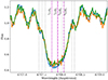 |
Fig. A.1. ESPRESSO spectra of DM Tau around the Li 6708 Å feature. Positions of the Li isotope resonance D lines are indicated by the magenta lines. Potential blends from elements with a lower abundance are marked by the black lines. From left to right, these are Fe I, V I, Cr I, Si I, V I, FeI, and Fe I (Franciosini et al. 2022a). |
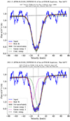 |
Fig. A.2. Example Gaussian fits to the ESPRESSO spectra of DM Tau for the Li absorption line. The central positions of the Gaussian(s) are indicated by the vertical dashed line(s). |
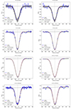 |
Fig. A.3. Further example Gaussian fits to the Li absorption line for the different instruments used. The central positions of the Gaussian fits are indicated by the vertical dashed lines. Zero km/s corresponds to a wavelength of 6708 Å, and the Li centroid positions were calculated with respect to this reference position. |
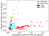 |
Fig. A.4. Calculated standard errors for the RV measurements and the Gaussian centre position from the best-fit model to the absorption line. |
Appendix B: Comparison of further stellar properties
We include figures showing comparison of the Teff of the young star sample measured with ROTFIT for the PENELLOPE data and those from TIC (Fig. B.1). We find similar values of up to a few 100K lower in some spectrally derived temperatures, as in Gangi et al. (2022) and Flores et al. (2022). We also include correlation plots for observed Li position versus veiling (Fig. B.2), and log g (Fig. B.3) of the YSOs. Veiling and log g measurements for the PENELLOPE sample are from ROTFIT, and log g values for the HARPS targets are from TIC. The Pearson correlation coefficients for each are three to six orders of magnitude less significant than the correlation between the Li position and Teff, as reported in the main text.
 |
Fig. B.1. Comparison of the temperature differences from the ROTFIT-derived spectrum measurements of PENELLOPE to those from TIC. Points are coloured by the mean Li centroid position. |
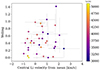 |
Fig. B.2. Comparison of the veiling measured with ROTFIT of the PENELLOPE spectra and the mean central velocity of the Li feature for each target. Veiling is measured within 50 nm of the mean Li position. Points are coloured by the Teff measurement from ROTFIT. The Pearson correlation coefficients are r = 0.22 and p = 0.21 |
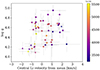 |
Fig. B.3. Comparison of log g and mean central velocity of the Li feature for each target. Circles are ROTFIT measurements of the PENELLOPE spectra, and triangles are from TIC. Points are coloured by the respective Teff measurement. The Pearson correlation coefficients are r = 0.35 and p = 0.02. |
Appendix C: Individual observational results
We discuss the spread of the observed Li position from repeated observations of individual targets in more detail. Figure C.1 shows a box plot for the measured Li position of each target. TW Hya and GM Aur were observed most frequently with the VLT and show good agreement between the X-Shooter and ESPRESSO measured Li positions. Some targets have fewer observations, but the positional differences between the X-Shooter and ESPRESSO/UVES observations are larger (see Tab C.1). This may be due to differences in instrument resolution (as previously described) or to further inherent variability because these dispersions do not exceed the range of those with more repeated observations.
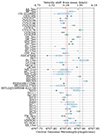 |
Fig. C.1. Li measurement for each target. The mean position of the Li feature is indicated by the dashed red line. As in Fig. 1, the boxes cover the inter-quartile range, and the whiskers extend to 1.5 times this range. Outliers are indicated by the circles. Each of the PENELLOPE targets has at least one X-Shooter observation in addition to their UVES and ESPRESSO observations. |
Summary of observations by instrument, mean RVs, and Li shift (from the overall mean position) with standard deviations across observations as measured with STAR-MELT. For the ESPRESSO, UVES, and X-Shooter spectra, Teff s are also the mean values measured across all PENELLOPE observations with ROTFIT, unless indicated by an asterisk. For these targets and the HARPS targets, Teff s are from TIC (Stassun et al. 2019).
The stars LY Lup (15), HD147048 (16), MS Lup (16), and MZ Lup (10) have the most repeated observations with HARPS. We checked the time variation of the measured Li position versus the reported photometric rotational periods for these stars and found that the rotational period for LY Lup (see Fig. C.2) and HD147048 was recovered by the Lomb-Scargle periodogram (LSP; for implementation details, see Campbell-White et al. 2021), but shorter-term variations had higher power. This suggests that the variations are more rapid than those of the overall rotation. These periodicities are tentative (non-negligible false-alarm probabilities) due to the small number of data points. The phase plots nevertheless illustrate the spread in variations well. The reported periods of MS Lup and MZ Lup (see Fig. C.3) were not shown at significant power on the LSP. Multiple periods shorter than a day were found, again at low significance. We obtained repeated observations per night and covered more than the rotational periods in each case, therefore these results suggest that the position of the Li centroid perhaps varies on timescales shorter than typical rotation periods of YSOs.
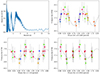 |
Fig. C.2. LY Lup LSP and phase-folded Li positions (procedure as described in Campbell-White et al. (2021). The velocities are those measured from the reference wavelength of 6708 Å and are already corrected for stellar RV. The phase plots therefore represent the relative shift in Li position. Points are coloured by observations corresponding to different phases. The photometric period of 2.84d from Kiraga (2012) is one of the peaks from the periodogram. False-alarm probabilities are lower for the shorter periods (∼ 20%), but the significance is still low due to the number of data points. |
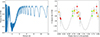 |
Fig. C.3. As Fig. C.2 for MZ Lup. The photometric period of 4.47d from Kiraga (2012) is not clearly recovered in the periodogram. A high-power period of 0.53d (false-alarm probability of 10%) is shown. |
All Tables
Line centres and oscillator strengths of the components of the Li Iλ6708 Å line (Morton 2003).
Summary of observations by instrument, mean RVs, and Li shift (from the overall mean position) with standard deviations across observations as measured with STAR-MELT. For the ESPRESSO, UVES, and X-Shooter spectra, Teff s are also the mean values measured across all PENELLOPE observations with ROTFIT, unless indicated by an asterisk. For these targets and the HARPS targets, Teff s are from TIC (Stassun et al. 2019).
All Figures
|
Fig. 1. Box plot of the resulting central wavelength position from fitting all of the PENELLOPE VLT (ESPRESSO, UVES, X-shooter) and the further HARPS YSO spectra. The boxes extend from the lower to upper quartile values of the data, with a green line at the median. The whiskers extend to 1.5 times the box range. Outliers are indicated by circles. The mean central wavelength position is marked by the dashed magenta line. Positions of the 7Li D1, D2, and 6Li D2 lines are indicated by the dashed and dash-dotted black lines. The grey shaded area indicates the range of values of the Li I line centres that were used as reference for the RV calculations in previous works. |
| In the text | |
|
Fig. 2. Teff vs. velocity difference from the mean measured Li centroid position. Stars indicate the mean measured position for each target. The shaded boxes show the 1σ spread of measurements. Circles indicate that Teff measurements are from ROFIT/PENELLOPE spectra, and triangles are taken from the TESS input catalogue. We note an anti-correlation (r = −0.58) between Teff and mean position: lower Teff stars show more redshifted central values. The total velocity error bars arise from adding the standard errors of the RV and Gaussian centre measurements in quadrature. Faded markers and error bars are measurements with total velocity errors 0.75 km s−1. The mean measured Li centroid and positions of the D line components are indicated in the top histogram. |
| In the text | |
|
Fig. A.1. ESPRESSO spectra of DM Tau around the Li 6708 Å feature. Positions of the Li isotope resonance D lines are indicated by the magenta lines. Potential blends from elements with a lower abundance are marked by the black lines. From left to right, these are Fe I, V I, Cr I, Si I, V I, FeI, and Fe I (Franciosini et al. 2022a). |
| In the text | |
|
Fig. A.2. Example Gaussian fits to the ESPRESSO spectra of DM Tau for the Li absorption line. The central positions of the Gaussian(s) are indicated by the vertical dashed line(s). |
| In the text | |
|
Fig. A.3. Further example Gaussian fits to the Li absorption line for the different instruments used. The central positions of the Gaussian fits are indicated by the vertical dashed lines. Zero km/s corresponds to a wavelength of 6708 Å, and the Li centroid positions were calculated with respect to this reference position. |
| In the text | |
|
Fig. A.4. Calculated standard errors for the RV measurements and the Gaussian centre position from the best-fit model to the absorption line. |
| In the text | |
|
Fig. B.1. Comparison of the temperature differences from the ROTFIT-derived spectrum measurements of PENELLOPE to those from TIC. Points are coloured by the mean Li centroid position. |
| In the text | |
|
Fig. B.2. Comparison of the veiling measured with ROTFIT of the PENELLOPE spectra and the mean central velocity of the Li feature for each target. Veiling is measured within 50 nm of the mean Li position. Points are coloured by the Teff measurement from ROTFIT. The Pearson correlation coefficients are r = 0.22 and p = 0.21 |
| In the text | |
|
Fig. B.3. Comparison of log g and mean central velocity of the Li feature for each target. Circles are ROTFIT measurements of the PENELLOPE spectra, and triangles are from TIC. Points are coloured by the respective Teff measurement. The Pearson correlation coefficients are r = 0.35 and p = 0.02. |
| In the text | |
|
Fig. C.1. Li measurement for each target. The mean position of the Li feature is indicated by the dashed red line. As in Fig. 1, the boxes cover the inter-quartile range, and the whiskers extend to 1.5 times this range. Outliers are indicated by the circles. Each of the PENELLOPE targets has at least one X-Shooter observation in addition to their UVES and ESPRESSO observations. |
| In the text | |
|
Fig. C.2. LY Lup LSP and phase-folded Li positions (procedure as described in Campbell-White et al. (2021). The velocities are those measured from the reference wavelength of 6708 Å and are already corrected for stellar RV. The phase plots therefore represent the relative shift in Li position. Points are coloured by observations corresponding to different phases. The photometric period of 2.84d from Kiraga (2012) is one of the peaks from the periodogram. False-alarm probabilities are lower for the shorter periods (∼ 20%), but the significance is still low due to the number of data points. |
| In the text | |
|
Fig. C.3. As Fig. C.2 for MZ Lup. The photometric period of 4.47d from Kiraga (2012) is not clearly recovered in the periodogram. A high-power period of 0.53d (false-alarm probability of 10%) is shown. |
| In the text | |
Current usage metrics show cumulative count of Article Views (full-text article views including HTML views, PDF and ePub downloads, according to the available data) and Abstracts Views on Vision4Press platform.
Data correspond to usage on the plateform after 2015. The current usage metrics is available 48-96 hours after online publication and is updated daily on week days.
Initial download of the metrics may take a while.