| Issue |
A&A
Volume 673, May 2023
|
|
|---|---|---|
| Article Number | A107 | |
| Number of page(s) | 26 | |
| Section | Interstellar and circumstellar matter | |
| DOI | https://doi.org/10.1051/0004-6361/202245406 | |
| Published online | 17 May 2023 | |
Toward nebular spectral modeling of magnetar-powered supernovae
The Oskar Klein Centre, Department of Astronomy, Stockholm University, Albanova
10691,
Stockholm,
Sweden
e-mail: This email address is being protected from spambots. You need JavaScript enabled to view it.
Received:
8
November
2022
Accepted:
13
March
2023
Abstract
Context. Many energetic supernovae (SNe) are thought to be powered by the rotational energy of a highly magnetized, rapidly rotating neutron star. The emission from the associated luminous pulsar wind nebula (PWN) can photoionize the SN ejecta, leading to a nebular spectrum of the ejecta with signatures that might reveal the PWN. SN 2012au is hypothesized to be one such SN.
Aims. We investigate the impact of different ejecta and PWN parameters on the SN nebular spectrum, and test whether any photoionization models are consistent with SN 2012au. We study how constraints from the nebular phase can be linked into modeling of the diffusion phase and the radio emission of the magnetar.
Methods. We present a suite of late-time (1–6 yr) spectral simulations of SN ejecta powered by an inner PWN. Over a large grid of one-zone models, we study the behavior of the physical state and line emission of the SN as the PWN luminosity (LPWN), the injected spectral energy distribution (SED) temperature (TPWN), the ejecta mass (Mej), and the composition (pure O or realistic) vary. We discuss the resulting emission in the context of the observed behavior of SN 2012au, a strong candidate for a PWN-powered SN. We used optical light-curve models and broadband PWN models to predict possible radio emission from SN 2012au.
Results. The SN nebular spectrum varies as TPWN varies because the ejecta become less ionized as TPWN increases. Ejecta models with low mass and high PWN power obtain runaway ionization for O I, and in extreme cases, also O II, causing a sharp decrease in their ion fraction over a small change in the parameter space. Certain models can reproduce the oxygen line luminosities of SN 2012au reasonably well at individual epochs, but we find no model that fits over the whole time evolution. This is likely due to uncertainties and simplifications in the model setup. Using our derived constraints from the nebular phase, we predict that the magnetar powering SN 2012au had an initial rotation period ~15 ms, and it is expected to be a strong radio source (F > 100 μJy) for decades.
Key words: radiative transfer / stars: magnetars / supernovae: general / supernovae: individual: SN 2012au
© The Authors 2023
 Open Access article, published by EDP Sciences, under the terms of the Creative Commons Attribution License (https://creativecommons.org/licenses/by/4.0), which permits unrestricted use, distribution, and reproduction in any medium, provided the original work is properly cited.
This article is published in open access under the Subscribe to Open model. This email address is being protected from spambots. You need JavaScript enabled to view it. to support open access publication.
1 Introduction
Recent optical transient surveys have revealed several classes of core-collapse SNe (CCSNe) that are more luminous and energetic than predicted by standard SN models. These include hydrogen-poor superluminous SNe (SLSNe), which are the brightest known optical transients. SLSNe radiate ~100 times more energy than a typical SN (Gal-Yam 2012; Nicholl 2021). The CCSNe also include broad-line Type Ic SNe (SNe Ic-BL), which are slightly overluminous, and their inferred kinetic are higher than the canonical SN explosion energy of 1051 erg (e.g., Taddia et al. 2019). Some SNe Ic-BL have been associated with long-duration gamma-ray bursts (LGRBs; Cano et al. 2017), while a small number of SLSNe have been associated with ultra-long gamma-ray bursts (ULGRBS; Gendre et al. 2013; Nakauchi et al. 2013; Levan et al. 2014), although strong radio and X-ray constraints show that jet formation in SLSNe is rare (Coppejans et al. 2018; Margutti et al. 2018). SLSNe and SNe Ic-BL also tend to have similar spectral features both at early (Pastorello et al. 2010; Inserra et al. 2013; Nicholl et al. 2013; Blanchard et al. 2019) and late phases (Milisavljevic et al. 2013; Jerkstrand et al. 2017; Nicholl et al. 2017), and they have similar host-galaxies (Lunnan et al. 2014; Leloudas et al. 2015b; Angus et al. 2016; Schulze et al. 2018; ∅rum et al. 2020).
Because of these similarities, many studies have suggested that these two SN classes could be powered by the same mechanism (Metzger et al. 2015; Ioka et al. 2016; Kashiyama et al. 2016; Margalit et al. 2018; Suzuki & Maeda 2021). SLSNe have been suggested to arise from pair-instability explosions (Barkat et al. 1967; Gal-Yam et al. 2009), pulsational pair-instability explosions (Heger & Woosley 2002), or by interaction with the circumstellar medium (CSM; Chatzopoulos et al. 2012; Ginzburg & Balberg 2012), but neither model scenario has been demonstrated to be able to produce both light curves and spectra. Another suggested powering mechanism is fallback onto a newly formed black hole (Dexter & Kasen 2013), but the accretion rate needed to produce a SLSN is unphysically high in most cases (Moriya et al. 2018). Another model that seems consistent with both SLSNe and SNe Ic-BL light curves is the magnetar-driven model (Kasen & Bildsten 2010; Woosley 2010), in which the rotational energy of a highly magnetized, rapidly rotating neutron star powers a luminous PWN. This exerts a pressure on the ejecta, accelerating it, and also produces broadband emission that is thermalized in the ejecta, increasing the temperature and ionization of the gas and the luminosity of the SN.
The magnetar engine model makes several multiwavelength predictions that can be used to test it and characterize the magnetar further. The PWN is expected to be bright in both radio and X-rays at late times (Murase et al. 2015; Kashiyama et al. 2016; Omand et al. 2018), and a few observations have been performed (e.g., Margutti et al. 2018; Eftekhari et al. 2021; Murase et al. 2021). So far, only one promising PWN candidate has been detected in radio: PTFlOhgi (Eftekhari et al. 2019; Law et al. 2019; Mondal et al. 2020; Hatsukade et al. 2021). An infrared (IR) excess was predicted by Omand et al. (2019) because the PWN emission heats newly formed dust in the ejecta, which has been detected in four SLSNe (Chen et al. 2021; Sun et al. 2022), although it can also be illuminated by the SN in an IR echo (Bode & Evans 1980; Dwek 1983) or heated through shock interaction (Smith et al. 2008; Fox et al. 2010; Sarangi et al. 2018), and collapsar models also predict an IR excess due to r-process nucleosynthesis in the accretion disk (Barnes & Metzger 2022; Anand et al. 2023). Polarization has also been observed in several SLSNe. This might stem either be from a central engine (Inserra et al. 2016; Saito et al. 2020) or from CSM interaction (Pursiainen et al. 2022), but other SLSNe are unpolarized (Leloudas et al. 2015a; Lee 2019, 2020; Poidevin et al. 2022, 2023), so this signal is not ubiquitous.
At later times, SN ejecta become more transparent, and emission from the metal-rich core can reveal important information about the origin and explosion of the star. This phase is often referred to the nebular phase, even though radiative transfer effects can still operate for many years or decades. Spectroscopic observations of SLSNe and Ic-BL SNe in their nebular phase are limited because they are relatively rare and the distances are often significant. A few relatively nearby events have been well studied (Gal-Yam et al. 2009; Chen et al. 2015; Yan et al. 2015, 2017; Nicholl et al. 2016, 2018; Lunnan et al. 2016, 2018; Jerkstrand et al. 2017; Quimby et al. 2018; Blanchard et al. 2021; West et al. 2023), leading to some small-scale statistical analysis (Nicholl et al. 2019). Both SLSNe and SNe Ic-BL show strong [O I] λλ6300, 6364 and [Ca II] λλ7291, 7323 emission, and SLSNe also show strong O I λ7774 emission and an elevated flux around 5000 Å, where [Fe II] is thought to dominate (Nicholl et al. 2019). This has also occurred in some SNe Ic-BL, however, such as SN 1998bw (Mazzali et al. 2001). Some SLSNe also show [O III] lines (Lunnan et al. 2016; Jerkstrand et al. 2017; Yan et al. 2017) and possibly [O II] as well.
Efforts to model the nebular spectra of these exotic SNe are limited so far. Observed spectra are inconsistent with pair-instability spectral models (Dessart et al. 2013; Jerkstrand et al. 2016) because these massive, 56Ni-powered SNe tend to produce cool and neutral ejecta, with red, strongly line-blanked spectra with narrow lines of species such as Fe I and Si I. This contradicts even qualitatively with the observed spectra of SLSN such as SN 2007bi and PTF12dam (Gal-Yam et al. 2009; Chen et al. 2015), which are blue, with broad lines. Other studies have tried to mimic the effects of additional late-time energy deposition, for instance, by a magnetar, into normal CCSN ejecta (Dessart et al. 2012; Jerkstrand et al. 2017; Dessart 2018, 2019). These models are more successful, mostly because the ejecta masses are lower and there is less line-blanketing iron. They treat the magnetar power, however, as either a purely thermal on-the-spot energy injection or in the same manner as radioactive decay. This approach may miss effects of increased photoionization and does not probe the PWN spectral energy distribution (SED), which is not yet well constrained and has strong implications for multi-wavelength studies. Nebular spectra can also probe clumping in the ejecta, and studies have inferred a high amount of clumping for both normal stripped envelope SNe (Taubenberger et al. 2009) and SLSNe (Jerkstrand et al. 2017; Nicholl et al. 2019; Dessart 2019).
In this paper, we develop the spectral synthesis code SUMO (Jerkstrand et al. 2011, 2012) to enable it to handle powering by high-energy radiation from a PWN. We use this code to investigate spectral formation over a parameter space relevant for SLSNe and Ic-BL SNe. We study the physical processes occurring in the ejecta and search for distinct predictions for emergent spectra that could reveal the presence of a central magnetar. In particular, we compare the models to observations of SN 2012au, a peculiar luminous stripped-envelope (Type Ib) SN with spectra taken at about one year and at about six years (Milisavljevic et al. 2013, 2018; Takaki et al. 2013; Pandey et al. 2021).
The paper is structured as follows. Section 2 summarizes the numerical model and model setup. Section 3 presents some general theory regarding the formation of oxygen lines. In Sect. 4 we overview previous observations of SN 2012au. Results are presented in Sect. 5, and their implications are discussed in Sect. 6. Finally, a summary is given in Sect. 7.
2 Modeling overview
2.1 SUMO
Non-local thermodynamic equilibrium (NLTE) spectral synthesis was performed using the code SUMO (Jerkstrand et al. 2011, 2012; Jerkstrand 2017), which takes an input composition and input density as a function of ejecta velocity; solves for the temperature, ionic abundances, atomic level populations, and the radiation field; and uses these to compute the emergent SN spectrum. SUMO is specialized to the late NLTE phase of the SN. It can compute the physical state of the ejecta either in steady state or time dependently (Pognan et al. 2022b). The code currently treats 22 elements between hydrogen and nickel, several r-process elements (Pognan et al. 2022a), and several molecules (Liljegren et al. 2020, 2022). An arbitrary number of ionization stages can now be treated. In this study, the first four stages were allowed for. Code updates for this study are given in Appendix A.
2.2 Model setup
We explored two types of compositions. The most abundant element in virtually all stripped-envelope CCSN models is oxygen. Oxygen provides the dominant lines in the 6y spectrum of SN 2012au, with strong emission from all its first three ionization stages. The first composition therefore was pure oxygen.
The second composition was taken from a stellar evolution and explosion model of a MZAMS = 25 M⊙ progenitor CCSN from Woosley & Heger (2007). This progenitor has a CO core of 6.8 M⊙, 1.8 M⊙ of which forms a compact object, and 5.0 M⊙ of nuclear processed material is ejected in the SN. For this model, we assumed that all the material becomes homogeneously mixed. Whereas complete microscopic mixing is not indicated in normal SNe (Fransson & Chevalier 1989; Jerkstrand 2017), stronger mixing may be induced when a powerful PWN is present (see, e.g., simulations by Chen et al. 2020; Suzuki & Maeda 2021). Since the ejecta mass Mej can vary in this study, the mass fractions were held constant, and element masses were scaled with ejecta mass. The mass fractions for this model are listed in Table 1.
The short mean-free path of X-rays and UV radiation means that morphology details are likely important for SNe that are powered by PWNe. One-dimensional photoionization models show that the ejecta develop regions of different ionization states (e.g., Chevalier & Fransson 1992). This is in contrast to a radioactivity-powered SNe. The mean-free path of gamma rays in these SNe is similar to the ejecta scale in the nebular phase, and the gamma-ray field strength therefore varies little or only moderately.
On the other hand, the strong Rayleigh-Taylor mixing seen in multidimensional simulations of engine-driven SNe (Chen et al. 2020; Suzuki & Maeda 2021) calls the applicability of stratified multizone models in 1D into question. The onion-shell structure is probably such a poor representation of the real morphology that gains in accuracy are not obvious. As illustrated to some extent by the images of the Crab nebula, the synchrotrongenerating regions may become mixed in velocity space with clumps and filaments of ejecta. If this mixing is strong enough, the final situation may be closer to a one-zone setup than to a stratified 1D ejecta.
As a starting point, we mostly explored one-zone models for our two compositions. However, in Sect. 5.3, we also explore the effects of zoning (in 1D) using one of the models. This analysis shows that when 1D ionization stratification is allowed, differences of a factor of a few can be expected in the main oxygen emission lines. We then use this information to assess which part of the parameter space of the one-zone models are viable for SN 2012au.
The shell in our model expands homologously between 2000 and 3000 km s−1. The inner boundary represents the contact discontinuity between the ejecta and the PWN. The inner boundary velocity is set from the low-velocity emission lines detected around one year in SN 2012au (Milisavljevic et al. 2013) by assuming that these lines are produced close to the contact discontinuity, while the outer boundary was chosen so that the single-zone density was similar to the density of the inner ejecta region, with a ρ ∝ v−6 density profile motivated by multidimensional numerical simulations of engine-driven SNe (Suzuki & Maeda 2017, 2019). This density profile is expected for SNe with a total engine energy greater than the SN explosion energy, injected over a timescale shorter than the diffusion time, and without significant early radiative losses dampening the efficiency of energy transport from the central ejecta to the outer layers (Suzuki & Maeda 2021). The shell had a constant density and a filling factor of 1. Clumping was not considered in this study.
The SED of the photons injected at the inner boundary, which represents the emission from the pulsar-wind nebula, is taken as a blackbody with a temperature TPWN and luminosity LPWN; the number of ionizing photons that were injected was proportional to  as long as TPWN was high enough for most of the photons to be ionizing. While a more realistic treatment would use a power law or broken power law to represent the broadband synchrotron emission, this would involve two or three parameters for the SED shape. By using a black-body SED instead, we limited the grid to introduce just a single further parameter. Furthermore, one of our goals is to understand the basic physical mechanisms at play. To this end, using blackbodies of different temperatures allowed us to study the connection between characteristic photon energies and resulting gas properties.
More complicated PWN models, such as those that calculate synchrotron emission and self-absorption, pair cascades, Compton and inverse Compton scattering, adiabatic cooling, and both internal and external attenuation (Murase et al. 2015, 2016), mostly still find that the SED resembles a broken power law in the IR to X-ray range (see Fig. 3 from Omand et al. (2018), e.g.) because these additional processes mostly affect the spectrum at radio and hard X-ray/gamma ray wavelengths. Vurm & Metzger (2021) showed that to reproduce the late-time light-curve decay in SN 2015bn and SN 2017egm, the PWN spectrum must be dominated by inverse Compton-emission, and must mostly emit in X-rays and gamma rays. This scenario would predict extremely faint radio emission, however, which contradicts radio observations of PTF10hgi (Eftekhari et al. 2019; Law et al. 2019; Mondal et al. 2020; Hatsukade et al. 2021).
At t = 6 yr, we computed a model grid with LPWN = 1 × 1038−1 × 1040 erg s−1, TPWN = 105−106 K, Mej = 1.0−10.0 M⊙, and either a pure oxygen or realistic SN Ic composition (as described above). At t = 320 days, we computed a smaller grid motivated by the results at t = 6 yr. The models are named by time (approximate in years), composition, Mej, LPWN, and TPWN: an example is 6Ic-4-1e40-1e5.
We investigated a range of ejecta masses 1–10 M⊙, motivated by both the mass range estimated for SN 2012au in previous studies (Takaki et al. 2013; Milisavljevic et al. 2013; Pandey et al. 2021) and by the mass range estimated for the Ic-BL population in previous sample studies (Taddia et al. 2019; Corsi et al. 2022; Anand et al. 2023). This mass range and the velocities chosen give kinetic energies of ~1050−51 erg, which is lower than the energy expected for a typical CCSN. A lower kinetic energy will cause a higher ejecta density, which may cause the temperature and ionization to be lower (Dessart 2019). When the difference is large, the models may be interpreted to represent the line-forming region, in which the inner ejecta lie close to the edge of the PWN and receive its input.
The luminosity of a PWN at late times is roughly
 (1)
(1)
 (2)
(2)
is the initial PWN luminosity, and tSD is the pulsar spin-down time. The rotational energy Erot and spin-down time of the pulsar are related to the initial pulsar spin period P0 and pulsar magnetic field B (assumed to be constant in time) by
 (3)
(3)
 (4)
(4)
Combining these gives a PWN luminosity of
 (5)
(5)
The typical magnetic field of a rapidly rotating pulsar that reproduces a Ic-BL SN light curve if the diffusion phase is magnetar powered is estimated to be ~5 × 10¹⁴ G (Kashiyama et al. 2016), which gives a PWN luminosity at six years of ~1039 erg s−1. This motivated the range of PWN luminosities we examined.
The characteristic synchrotron energy vb in a PWN at which vFv peaks is given by (Murase et al. 2021)
 (6)
(6)
where єB is the fraction of spin-down energy carried by nebular magnetic fields, and γb is the average electron injection Lorentz factor. The values shown in Eq. (6) are typical of those found from modeling Galactic PWNe, including the Crab nebula (Kennel & Coroniti 1984; Tanaka & Takahara 2010, 2013). However, these values, as well as those for spectral indices, are not well constrained for highly luminous newborn PWNe, but there is some evidence that the value differs from that of Galactic PWNe (Law et al. 2019; Eftekhari et al. 2021; Murase et al. 2021; Vurm & Metzger 2021). For these default parameters, this gives a characteristic photon energy of ~ 130 eV, which corresponds to the peak of a blackbody with a temperature of ~5 × 10⁵ K. This motivated the injection range of the SED temperatures we examined. We allowed three values for TPWN: 1 × 10⁵, 3 × 10⁵, and 1 × 10⁶ K, which correspond to characteristic photon energies (2.8kT) of 24, 72, and 240 eV, respectively. These energies are all high enough for most of the photons to be able to photoionize oxygen.
A few pieces of physics are relevant to an engine-driven SN, but are not yet treated correctly by SUMO. The most prominent physics is inner-shell ionizations. While electron- and photon-impact ionization partially considers contribution from inner shells, their contribution to ionization rates is approximate because we did not follow Auger and fluorescence processes in detail. We therefore avoided hard X-ray illumination of the ejecta to avoid these inner shell processes. This restricted us to using TPWN ≲ 106 K. When these processes are better treated, we will be able to explore higher SED temperatures, more realistic broadband injection spectra, and Compton-dominated spectra (Vurm & Metzger 2021). We also assumed that photo-electrons are fully thermalized, ignoring that they might ionize or excite the gas. This approximation should be reasonable for this study because no hard X-rays were injected because photo-electrons typically lack the energy to further ionize the ejecta. The other processes may be important for a more realistic PWN spectrum, however.
Composition of the realistic Ic model.
3 Formation of oxygen emission lines
The strength of the oxygen emission lines we studied depends on the parameters of the atomic transitions that correspond to the observed lines. The emissivity of a line is in general given by
 (7)
(7)
where nu is the population of the excited state for the line transition, A is the spontaneous radiative decay rate, and βS is the Sobolev escape probability (which we take to be unity for the analysis in this section, which corresponds to optically thin lines). The rate equilibrium equation for a two-level system with thermal collisional alone and spontaneous radiative decay terms is
 (8)
(8)
where  is the collisional excitation rate;
  is the collisional deexcitation rate; ng ≈ nion is the ground-state population; ne is the electron density; gdown and gup are the multiplicities of the ground and excited states, respectively; ϒ(T) is the effective collision strength, which is dependent on the cross-section function for the transition, but normally has a weak temperature dependence (Jerkstrand 2017), and so we took it to be constant; and c1 is also a constant. The excitation temperature Texc = Eexc/kB is the temperature that corresponds to the excitation energy for the transition. Solving for nuA gives
 (9)
(9)
From this equation, we find that the line luminosity is proportional to the ion density; decreases exponentially when the temperature is below the excitation temperature; and depends on the atomic parameters ϒ and A, and, at low electron densities, on ne. The quantity A/ (c1 ϒ) is known as the critical density ncrit, which is the cutoff between local thermodynamic equilibrium (LTE) and NLTE. If ne ≫ ncrit, the system is in LTE and the line emissivity is
 (10)
(10)
proportional to A, while if ne ≪ ncrit, then the line emissivity is
 (11)
(11)
proportional to ϒne. A schematic dependence of the third line-luminosity factor in Eq. (9), (putting gdown/gup = 1 for simplicity, so c1ϒne/(1 + c1ϒne/A)) on ne, A, and ϒ is shown in Fig. 1. For the same Texc, the lines with the same A values will show the same luminosity in the high ne (LTE) limit, the lines with the same ϒ values will show the same luminosity in the low ne limit, and the lines with the same A/ϒ value will have the same value of ncrit. The values of these properties for the [O I], [O II], and [O III] forbidden lines examined in this study are shown in Table 2.
[O I] λλ 6300, 6364. The [O I] λλ 6300, 6364 line has the lowest excitation temperature of any of the lines we studied, meaning that the transition can occur at lower ejecta temperatures than [O II] and [O III]. However, it has lower A and ϒ values, which means that apart from the exponential temperature term, its intrinsic emissivity is weaker than [O II] and [O III] both in LTE and NLTE. With its A/ϒ ~ 0.1, it has a critical density of ncrit = 3.8 × 106 cm−3. At 6y, the electron density of all our models is below this, meaning that the line will form in NLTE. At one year, however, the ejecta electron density is typically higher than ncrit, so [O I] will then be in LTE. The line will dominate [O II] and [O III] either when the gas is mostly neutral, and/or when temperatures are low or moderate. For equal ion abundances (nOI = nOII = nOIII), it becomes stronger than [O II] for T ≲ 15 000 K, and stronger than [O III] for T ≲ 3000 K.
[O II] λλ 7319, 7330. The [O II] λλ 7319, 7330 line has the highest excitation temperature of any of the lines we studied, meaning that the transition will be strong only at high ejecta temperatures. Both its A value and its ϒ value are a factor of about ten higher than for [O I]: its critical density is therefore about the same, and it will be in LTE at 1y and NLTE at 6 yr. For equal ion abundances, it is stronger than [O III] for T ≳ 15,000 K in LTE because its A value is ten times higher. As its collision strength is similar to [O III], it is always weaker in NLTE.
[O III] λλ 4959, 5007. The [O III] λλ 4959, 5007 line has an excitation temperature that is slightly higher than [O I], and the transition has the highest value of ϒ. With its A/ϒ ~ 0.01, it has a critical density about a factor of ten lower than [O I] and [O II], and it therefore remains longest in LTE. [O III] will be in LTE at one year and just transitions from LTE to NLTE around six years; the critical density is reached in models with ≳3 M⊙ of ejecta. For equal ion abundances, [O III] easily becomes strong in NLTE because its value of ϒ is high, but its excitation temperature is still quite low. It would also be comparable to [O I] in LTE because its A value is slightly higher.
Transition properties for the forbidden lines examined in this study.
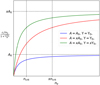 |
Fig. 1 Schematic showing the dependence of the third line-luminosity factor on ne, A, and ϒ. Lines with the same A values (red and green) will approach the same luminosity in the high ne (LTE) limit, lines with the same ϒ values (blue and red) show the same luminosity in the low ne limit, and lines with the same A/ϒ (blue and green) show the same value of ncrit, while ncrit for the red line is a factor of x larger. |
4 Summary of SN 2012au observations
The luminous SN Ib-pec SN 2012au was discovered on March 14, 2012 (Howerton et al. 2012) in NGC 4790 at 23.5 ± 0.5 Mpc (z = 0.0054 ± 0.0001). Milisavljevic et al. (2013), Takaki et al. (2013), and Pandey et al. (2021) presented a series of photometric and spectroscopic observations from pre-peak to one year post maximum. These studies estimated a quasi-bolometric peak luminosity of 6–7 × 1042 erg s−1, which is a factor of a few larger than a typical SN Ib/c. Arnett-type modeling of the diffusion phase gave best-fitting kinetic energies of (5–10) × 1051 erg (Milisavljevic et al. 2013; Takaki et al. 2013; Pandey et al. 2021). The studies all estimated an MNi of ≈0.3 M⊙ (assuming the diffusion phase is 56Co powered) and ejecta masses in the range 3–8 M⊙. Milisavljevic et al. (2013) and Kamble et al. (2014) both reported that the metallicity of the SN environment was Z ~ 1–2 Z⊙.
SN 2012au showed unusual spectroscopic evolution during its first year. Spectra taken around peak closely resemble SNe of Type Ib, such as SN 2008D (Soderberg et al. 2008), with prominent He I, Fe II, Si II, Ca II, Na I, and O I absorption features, although with velocities of ~2 × 10⁴ km s−1, which is much higher than normal SNe Ib. In the late photospheric phase (about 50 days post peak), the spectrum more closely resembles that of an SN Ic such as SN 1997dq (Matheson et al. 2001), although the observed velocities (~7000 km s−1) are still higher than those of typical SN Ib/c at this epoch. At about 110 days post peak, the [O I] and [Ca II] nebular emission lines appear (Takaki et al. 2013), and between then and ~250 days post peak, other emission lines appear (Milisavljevic et al. 2013), such as Mg I], Ca II H&K, Na I D, and O I. The nebular spectra also show persistent Fe II P-Cyg absorptions at ≲2000 km s−1 and an iron peak plateau between 4000 and 5600 Å, and the widths of the emission lines indicate two distinct emission regions, with Mg I] λ 4571; Na I λλ 5890, 5896; [O I] λλ 6300, 6364; and [Ca II] λλ 7291, 7324 all showing full width at half maximum (FWHM) velocities ≳4500 km s−1, and O I λ 7774, O 11.317 μm, and Mg I 1.503 μm all showing FWHM velocities ≈2000 km s−1. These features are more comparable to SLSN spectra at similar epochs, such as SN 2007bi (Gal-Yam et al. 2009). High imaging polarization values indicate asymmetry in the ejecta (Pandey et al. 2021).
Kamble et al. (2014) performed radio observations with the Jansky Very Large Array (VLA) between 5 and 37 GHz and X-ray observations with the Swift X-ray Telescope (XRT) between 0.3 and 10 keV within the first two months post-explosion. Emission was detected by both instruments. The flux of the bright radio emission was between 10 and 100 mJy and the radio energy budget was ~1047 erg. This is intermediate between SN 1998bw (Kulkarni et al. 1998; Li & Chevalier 1999) and SN 2002ap (Berger et al. 2002), which are two similarly energetic SNe (Iwamoto et al. 1998; Mazzali et al. 2002). The shock wave was estimated to have a velocity of 0.2c and a mass-loss rate of Ṁ = 3.6 × 10⁻⁶ M⊙ yr−1 for the wind velocity of 1000 km s−1 that was inferred for the progenitor. The lack of sharp features or discontinuities in the radio light curves suggest relatively smooth mass loss in the final few decades before the SN.
Milisavljevic et al. (2018) were able to obtain another optical spectrum at about six years post-explosion that only showed [O I], [Ca II]/[O II], [O III], and [S III] λλ 9069, 9531, with a possible detection of a broad but weak O I λ 7774 line. From 1y to 6y, the [O I] and [Ca II]/[O II] lines both narrowed from ≳4500 km s−1 to ~2300 km s−1 while maintaining roughly the same peak intensity ratio, while the O I line broadened significantly from ~2000 km s−1 while decreasing in peak intensity more significantly than [O I] and [Ca II]/[O II]. Milisavljevic et al. (2018) argued that this spectrum is inconsistent with those predicted by either radioactivity or SN-CSM interaction (e.g., Chugai & Chevalier 2006; Milisavljevic et al. 2015; Mauerhan et al. 2018), but can be consistent with PWN powering models (e.g., Chevalier & Fransson 1992). Milisavljevic et al. (2018) also obtained X-ray upper limits of LX < 2 × 1038 erg s−1 between 0.5 and 10 keV using the Chandra X-ray Observatory (CXO).
Stroh et al. (2021) were able to detect radio emission from SN 2012au at about seven years post-explosion with the VLA Sky Survey (VLASS). The signal was in the 2–4 GHz band and had a flux of 4.5 ± 0.3 mJy. They considered emission from CSM interaction, off-axis jets, and emergent PWNe, and concluded that the emission was likely from a PWN, similar to Milisavljevic et al. (2018).
The spectra of other SNe were taken at very late times as well (for a review, see Milisavljevic et al. 2012), but most of them, with the exception of the Type IIb SN 1993J (Filippenko et al. 1993) and the Type II-pec SN 1987A (Menzies et al. 1987; Chugai et al. 1996), are Type IIn or Type IIL SNe (for a review of their spectral evolution, see Chevalier & Fransson 1994), and all of them show clear signs of interaction with CSM. SN 2012au is unique as the only stripped envelope SN with spectra taken at very late times, and it is the only one without clear signs of strong CSM interaction.
5 Results
We present grids of one-zone models for the pure oxygen and realistic compositions, as well as a multizone model for one of our highest optical depth models. The overall goodness of fit for our models is evaluated with a model score
![Mathematical equation: $ {\rm{Score}}\,{\rm{ = }}\,\sum\limits_i {{{\left( {\log \,\left[ {{{{L_{{\rm{i,model}}}}} \over {{L_{{\rm{i}},{\rm{obs}}}}}}} \right]} \right)}^2},} $](/articles/aa/full_html/2023/05/aa45406-22/aa45406-22-eq19.png) (12)
(12)
where Li is the line luminosity, with i running over all the lines used to generate the score. We used a logarithm so that brighter lines did not overwhelm the score. A perfect match for a line will give a score of 0, and factors of 2, 5, and 10 difference in luminosity will give scores of ~0.1, ~0.5, and 1, respectively. We studied line luminosities as opposed to line ratios, which are insensitive to distance uncertainties, because certain ejecta properties do not scale simply with certain parameters; for example, increasing LPWN to increase the luminosity of two lines would also change the ionization structure of the ejecta (e.g., Jerkstrand et al. 2017).
The line luminosity was calculated for both observations and models using (Jerkstrand et al. 2017)
 (13)
(13)
where I1 and I2 are defined as the integral of the flux
 (14)
(14)
with λ0 and dλ1 being chosen to enclose as much line flux as possible without contamination from other lines in either model or observation, and we use dλ2 = 1.25dλ1. Values of λ0 and dλ1 are unique to each line and each epoch, but shared between model and observation. The values of dλ1 are given in Table 3.
The model spectra at six years were compared to the spectrum from Milisavljevic et al. (2018), which has clear detections of forbidden oxygen transitions [O I] λλ 6300, 6364 (hereafter referred to as [O I]), either [O II] λλ 7319, 7330 or [Ca II] λλ 7291, 7323 (hereafter referred to as [O II] and [Ca II]), and [O III] λλ 4959, 5007 (hereafter referred to as [O III]), and a possible weak detection of O I λ 7774 (hereafter referred to as O I). The model spectra were not corrected for dust extinction along the line of sight (which has E(B − V) < 0.1 mag (Milisavljevic et al. 2013). However, the model spectra were adjusted for extinction from dust formed within the SN by dividing the line luminosities by factors of 3.31, 3.37, and 2.10 for [O I], [O II], and [O III], respectively (Niculescu-Duvaz et al. 2022). The flux of the O I line was too low for strong constraints to be placed on dust formation, and therefore we assumed that this line is unaffected by dust. The spectra at one year were compared to observations from Milisavljevic et al. (2013), focusing mostly on the [O I] and O I lines because [O III] is not clearly detected and [Ca II] probably contributes to the [O II] line.
Values of dλ1 for each line and epoch used to determine the observed and model line luminosities.
5.1 Pure oxygen composition
5.1.1 Six years
The ejecta temperature and ion fractions for O I, O II, and O III over the grid are shown in Fig. 2. Models with a high ejecta mass and low engine luminosity are dominated by O I, and increasing luminosity and decreasing the ejecta mass shift the ionization balance more toward O II, which is more prominent in the middle of the grid, and O III, which is most prominent at low ejecta masses and high engine luminosities.
There is a sharp decrease in O I fraction as the engine luminosity increases and the ejecta mass decreases. This is due to runaway ionization, a sharp transition in the ionization balance solution as the radiation field strength exceeds a critical value (Jerkstrand et al. 2017). This is related but not identical to ionization breakout (Metzger et al. 2014), which refers to when the whole ejecta become optically thin at some wavelength due to ionization. Runaway ionization for O II can also be seen at the highest engine luminosity and lowest mass in the model grid, leading to an ejecta that is dominated by O III. Because the photons at low TPWN are already energetic enough to ionize both OI and O II (a 105 K blackbody peaks at 24 eV, and the PWN will have enough photons that are more energetic than their ionization potentials of 13.6 and 35 eV, respectively), the decrease in ionizing photon count as TPWN increases causes runaway ionization to occur only in models with comparatively higher engine luminosities and lower ejecta masses.
The ejecta temperature increases when the ejecta mass decreases, the engine luminosity increases, or the injection SED temperature increases. The temperature covers the range 1600–6300 K.
The dust-corrected model line luminosities of [O I], [O II], and [O III]; normalized to the observed line luminosities of 7.3 × 1037, 1.0 × 1038, and 1.4 × 1038 erg s−1, respectively; and the O I line luminosity normalized to the observational limit of 3.5 × 1037 erg s−1 (Milisavljevic et al. 2018); are shown in Fig. 3. For all four lines, the PWN SED temperature has a clear effect on the line luminosities: the [O I], [O II], and [O III] luminosities increase with increasing TPWN, while the O I luminosity decreases. The O I luminosity is only too high in a small region of the parameter space with high LPWN, high Mej, and low TPWN, and this can likely exclude any models with TPWN < 105 K due to an overluminous O I line.
Although some features can easily be related to the ion fractions from Fig. 2, such as the decrease in [O I] luminosity due to the runaway ionization of O I, the line luminosities are not a simple function of the ion fractions (Sect. 3). The [O I] line luminosity roughly traces the ionization fraction, but is stronger in the high-mass regime with high engine luminosity when the ejecta is hottest while still mostly neutral. The [O II] line luminosity is only strong when the ejecta temperature is high due to the high excitation energy of the [O II] transition. Both the [O I] and [O II] lines also show a strong dependence on ejecta mass that is strongest in high-mass ejecta. The reason is that both lines are in NLTE and show luminosities  . The [O III] line is transitioning between LTE and NLTE, and it dependence on ejecta mass is weaker than for [O I] and [O III]. It is strongest in hot, highly ionized ejecta.
The goodness-of-fit score for each model, generated from Eq. (12) with [O I], [O II], and [O III] contributing, is shown in Fig. 4. None of the models with an engine luminosity <5 × 1038 erg s−1 provide a very good fit to the data, highlighting the need for sufficient energy injection to reproduce the spectrum. The best-fit models generally have higher ejecta masses and higher engine luminosities, but increasing TPWN causes the best-fit models to decrease in ejecta mass and engine luminosity. However, within this simple model, we find that engine luminosities ~ (1–5) × 1039 erg s−1 and ejecta masses ~1.5–6 M⊙ reproduce the spectrum best.
The two best-fitting spectra for each value of TPWN are shown in Fig. 5. Four of these six models are qualitatively unsatisfactory: the [O I] luminosity of 6O-4-2e39-3e5, 6O-6-5e39-3e5, and 6O-2.5-2e39-1e6 is higher than their [O III] luminosity (in contrast to observations), and the O I 7774 Å and 8446 Å emission of 6O-6-5e39-1e5 is significantly higher than the observed background. The other two models, 6O-4-2e39-1e5 and 6O-1.5-1e39-1e6, are able to reproduce the [O III] and [O I] luminosities to within a factor of ~ about two, although they both underestimate the [O II] luminosity. This may be due to possible contamination from the [Ca II] λλ 7291, 7323 doublet in the observed spectrum. We tentatively refer to the 6O-4-2e39-1e5 and 6O-1.5-1e39-1e6 the best-fit models for the pure oxygen composition at six years.
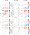 |
Fig. 2 Ion fractions of O I (top), O II (second row), and O III (third row), and the ejecta temperature Tej (bottom) in the simulations at six years for a pure oxygen composition at three different values of TPWN. The black contour denotes the regime with a low ejecta mass and high engine luminosity in which runaway ionization can occur for both O I and O II. |
5.1.2 One year
Based on the best-fit models at six years, we examined a smaller parameter space at one year to determine whether these models can also be consistent with observations at this phase. The engine luminosity was scaled higher, assuming vacuum dipole spin-down, but the injection SED temperature range was kept the same. The 1y grid was LPWN = 3 × 1040−3 × 1042 erg s−1, TPWN = 105–106 K, and Mej = 1.5–4 M⊙.
The ejecta temperature and ion fractions for O I, O II, and O III at one year are shown in Fig. 6. The dust-corrected model line luminosities of [O I] and O I normalized to the observed line luminosities of 7.1 × 1039 and 1.3 × 1039 erg s−1, respectively, and the [O II] and [O III] line luminosities normalized to the observational limits of 3.9 × 1039 and 8.6 × 1038 erg s−1. respectively (at 320 days post peak, Milisavljevic et al. 2013), are shown in Fig. 7.
The ionization state shows the same qualitative behavior as at six years. Runaway ionization occurs for O I in the regime of high engine luminosity and low ejecta mass. This regime shrinks as TPWN increases. Runaway ionization occurs for O II at the very highest engine luminosity and lowest ejecta mass in the model grid.
The ejecta temperature at one year shows the same qualitative behavior as at six years, increasing when the ejecta mass decreases, the engine luminosity increases, or the injection SED temperature increases. The temperature covers the range 4000 – 15 000 K. We recall that based on Sect. 3, this means that we stay in the regime in which a stronger [O II] than [O I] can only occur if O II is more abundant than O I. Furthermore, the [O III] to [O I] ratio roughly reflects their abundances.
The luminosity of [O I] most closely matches observations at low LPWN and along a narrow strip in the parameter space near the edge of the line at which runaway ionization occurs, which is poorly resolved in our model grid. The [O II] and [O III] luminosities trace the ionization factions fairly well and are high enough to exclude most of the high LPWN portion of the parameter space, although the [O II] emission is much stronger for higher TPWN, which results in high Tej. The line luminosity for O I is fairly consistent with observations over most of the model grid, and it is only weak when O II is experiencing runaway ionization.
The model scores based on the O I and [O I] lines (there are only upper limits for [O II] and [O III]) are shown in Fig. 8, and the two best-fitting spectra for each value of TPWN are shown in Fig. 9. In our one-zone approach, the model [O I] line is significantly narrower than the observed line, so that the peak intensity must be significantly higher to compensate for this. Spectra at TPWN = 106 K have strong [O II], [O III], and [O I] λ 5577 Å emission, as well as [O I] emission much stronger than observed. The models at TPWN = 3 × 10⁵ K show no obvious inadequacies, and fit the [O I] and O I lines within a factor of five, but the models at TPWN = 105 K fit both lines within a factor of two, making these the best-fitting models at one year.
While this is at the edge of the explored parameter space at one year, there are physical motivations for not extending the model grid to lower ejecta masses, engine luminosities, and injection SED temperatures. An ejecta mass of 1.5 M⊙ is not atypical of an SN Ic-BL (Taddia et al. 2019), but it is lower than previous studies have inferred for SN 2012au (Milisavljevic et al. 2013; Takaki et al. 2013; Pandey et al. 2021) and it is the lower limit that could reproduce the spectrum at six years. A lower engine luminosity at one year would imply that the spin-down rate would have to be slower than the vacuum dipole and have a breaking index n < 2.5, which is lower than that inferred for most pulsars (Parthasarathy et al. 2020) and for potential millisecond magnetars that have driven GRBs (Lasky et al. 2017; Şaşmaz Muş, et al. 2019). Finally, a lower injection SED temperature is inconsistent with the results found at six years regarding the OI line emission. A PWN is also expected to emit lower-energy photons at late times as the energy injection decreases and the nebula itself expands (see Eq. (6)), so that a lower TPWN at early times seems unphysical. It is likely that the PWN mainly emits in hard X-rays at one year, with a corresponding TPWN ≈ 107 K, but we cannot yet probe this regime because SUMO lacks inner shell processes (see Sect. 2.2).
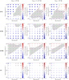 |
Fig. 3 Luminosity of the model [O I] (top), [O II] (second row), [O III] (third row), and O I (bottom) lines in units of the observed line luminosities and limits for SN 2012au at six years for a pure oxygen composition at three different values of TPWN. The green circled points represent where the model and observed values are within a factor of 2, the purple circles within a factor of 5, and the gray shaded region also within a factor of 5 for clarity. For O I (bottom panel), the black circled points represent where the model luminosity is more than a factor 2 higher than the observational upper limit. |
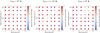 |
Fig. 4 Goodness-of-fit score for each model for the pure oxygen composition at six years based on the [O I], [O II], and [O III] lines. Lower scores indicate a better fit to the data (from Eq. (12), a perfect fit has a score of 0, all three lines off by a factor of two has a score of 0.27, and all three lines off by a factor of ten has a score of 3). The black circles indicate the two models with the lowest scores for each TPWN, which are plotted in Fig. 5. |
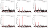 |
Fig. 5 Two best-fitting dust-corrected model spectra to SN 2012au for each value of TPWN at six years for a pure oxygen composition compared to the observed spectrum from Milisavljevic et al. (2018). Strong lines and features are labeled in the upper left plot. |
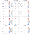 |
Fig. 6 Ion fractions of O I (top), O II (second row), and O III (third row), and the ejecta temperature Tej (bottom) in the simulations at one year for a pure oxygen composition at three different values of TPWN. The black contour denotes the regime with low ejecta mass and high engine luminosity in which runaway ionization can occur for both O I and O II. |
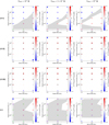 |
Fig. 7 Luminosity of the model [O I] (top), [O II] (second row), [O III] (third row), and O I (bottom) lines in units of the observed line luminosities and limits for SN 2012au at one year for a pure oxygen composition at three different values of TPWN. The green circled points represent where the model and observed values are within a factor of 2, the purple circles within a factor of 5, and the gray shaded region also within a factor of 5. The black circled points (for [O II] and [O III]) represent where the model luminosity is more than a factor of two higher than the observational limit. |
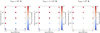 |
Fig. 8 Goodness-of-fit score for each model for the pure oxygen composition at one year based on the [O I] and O I lines. Lower scores indicate a better fit to the data (from Eq. (12), a perfect fit has a score of 0, both lines off by a factor of two has a score of 0.18, and both lines off by a factor of ten has score 2). The black circles indicate the two models with the lowest scores for each TPWN, which are plotted in Fig. 9. |
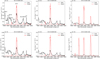 |
Fig. 9 Two best-fitting dust-corrected model spectra to SN 2012au for each value of TPWN at one year for a pure oxygen composition compared to the observed spectrum from Milisavljevic et al. (2013). Strong lines and features are labeled in the upper left plot. |
5.2 Realistic composition
5.2.1 Six years
We examined the results from simulations using the realistic stripped-envelope SN composition from Woosley & Heger (2007). The oxygen ion fractions and ejecta temperature at six years are shown in Fig. 10. They display a similar behavior as in the pure oxygen model (Fig. 2), with the most notable differences being that O I runaway ionization occurs at higher engine luminosities and lower ejecta masses, and that the ejecta temperature is much cooler (the range is here 400–6300 K compared to 1600–6300 K for pure oxygen) and shows a stronger dependence on TPWN.
The continuum-subtracted luminosities for the wavelength regions of each line, shown in Fig. 11, are much lower than in the pure oxygen case. This is driven by lower temperatures, as other elements now compete for the cooling and emission. Engine luminosity values close to 1039 erg s−1 that were sufficient to power the [O I] and [O III] lines in the oxygen composition are now insufficient, and values closer to 1040 erg s−1 are now preferred for all three lines. The [O I] line now fits best in the high-mass and high-luminosity regime, and only at high injection SED temperature, although a larger region of parameter space with higher ejecta masses and engine luminosities that may fit the [O I] line at lower values of TPWN might be possible. The [O II] line needs similar luminosities as the pure oxygen model to fit observations, but does not require ejecta masses that are as high, and there are no good fits at TPWN = 105 K, just like [O I]. The [O III] line, similar to the [O I] line, now fits at high luminosities, and the best-fit region is at increasing ejecta mass and decreasing engine luminosity as the injection SED temperature increases. The O I line luminosity is again too high in the high-mass high-luminosity regime, although the line luminosity decreases as the injection SED temperature increases. This means that the entire parameter grid is feasible at TPWN = 106 K. Overall, the realistic composition significantly favors higher values of TPWN because at TPWN = 105 K, none of the line luminosities are fit within a factor of two. This demonstrates the sensitivity of the emission to the microscopic composition.
The model scores based on the [O I], [O II], and [O III] lines are shown in Fig. 12. LPWN < 5 × 1039 erg s−1 are almost completely ruled out, and there are no low model scores at TPWN ≤ 3 × 10⁵ K. The two best-fitting spectra for TPWN = 106 K are shown in Fig. 13. Both models predict a high luminosity around 7300 Å, but this is coming from [Ca II] instead of [O II]. 6Ic-4-5e39-1e6 underestimates the [O III] luminosity, while 61c-4-1e40-1e6 overestimates it by about the same factor, and both are within a factor of two for the [O I] luminosity. These models also predict other detectable spectral features, particularly in the 6Ic-4-1e40-1e6 model, including the [S III] λλ 9069, 9531 doublet, of which the 9531 Å peak was observed; the S II λλ 6717, 6730 doublet; mixed Fe II and Fe III features around 4700 and 5300 Å; and a mixed Fe II and Ca II feature around 8600 Å. The prevalence of these features could either be due to differences in composition or to the extent of mixing between our models and SN 2012au. When we examined the oxygen emission alone, the models are roughly comparable in how well they reproduce the spectrum, but due to the prevalence of other features in 6Ic-4-1e40-1e6, we tentatively consider 6Ic-4-5e39-1e6 the best-fit model in this composition. This model is much less capable of reproducing the observed line ratios than 6O-4-2e39-1e5 and 6O-1.5-1e39-1e6, however, which are the best-fitting models in the pure oxygen composition.
The high LPWN needed to match the observed oxygen lines in the realistic composition compared to the pure oxygen composition is due to high levels of cooling outside of the observed wavelength range, which results is a much lower ejecta temperature (Fig. 10). For example, in the 6Ic-4-5e39-1e6 model, the emission from 4500–10 000 Å accounts for ~50% of the total cooling in the ejecta, and the rest comes mostly from Ne II, Ar II, Ar III, Fe II, Fe III, Ni II, and Ni III in the near- and mid-IR, as well as from Mg II, S II and Ca II in the UV. In lower LPWN models, such as the Ic composition-equivalent of the pure oxygen composition best-fit models, 6Ic-4-2e39-1e5 and 6Ic-1.5-1e39-1e6, <5% of cooling is in the optical band, with most of the emission coming from Ca II, and most of the rest of the emission is in the IR. Ne II is a particularly strong coolant in these models, with >50% of energy loss in the ejecta coming from the [Ne II] 12.8 μm line. This suggests that pulsar-driven SNe with strong mixing may be extremely bright IR sources at very late times, particularly in mid-IR. These might be interesting targets for the James Webb Space Telescope (JWST) as a test of both mixing in the SN and of the strength of the PWN, although emission from molecules (Liljegren et al. 2022) or pulsar-heated dust (Omand et al. 2019) might complicate the interpretation.
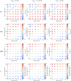 |
Fig. 10 Ion fractions of O I (top), O II (second row), and O III (third row), and the ejecta temperature Tej (bottom) in the simulations at six years for the realistic composition at three different values of TPWN. The black contour denotes the regime of low ejecta mass and high engine luminosity in which runaway ionization can occur for both O I and O II. |
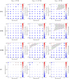 |
Fig. 11 Luminosity of the model [O I] (top), [O II] (second row), [O III] (third row), and O I (bottom) lines compared to the observed line luminosities and luminosity limits from SN 2012au at six years for the realistic composition at three different values of TPWN. The green circled points represent where the model and observed values are within a factor of 2two, the purple circles within a factor of five, and the gray shaded region also within a factor of five. The black circled points represent where the model luminosity is more than a factor of two higher than the observational limit. The grid includes luminosity from all elements in the wavelength regions in which these lines are emitted. |
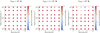 |
Fig. 12 Goodness-of-fit score for each model in the realistic composition at six years based on the [O I], [O II], and [O III] lines. Lower scores indicate a better fit to the data (from Eq. (12), a perfect fit has a score of 0, all three lines off by a factor of two has a score of 0.27, and all three lines off by a factor of ten has a score of 3). The black circles indicate the two models with the lowest scores for each TPWN, although TPWN = 105 K has no models with scores <3, and TPWN = 3 × 10⁵ K has no models with scores <2. The best-fitting models for TPWN = 106 K are plotted in Fig. 13 |
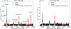 |
Fig. 13 Two best-fitting dust-corrected model spectra for TPWN = 106 K at six years for the realistic composition compared to the observed spectrum from Milisavljevic et al. (2018). The total model emission is shown in red, and the emission from only oxygen is shown in cyan. Strong lines and features are labeled in the left plot. |
5.2.2 One year
The oxygen ion fractions and ejecta temperature for the realistic composition at one year, using the same parameter grid as the pure oxygen composition, are shown in Fig. 14, and the normalized line luminosities are shown in Fig. 15. The ejecta temperatures are not significantly cooler than for the pure oxygen composition, in contrast to the differences seen at six years. Examination of the line luminosities for the [O II] and [O III] wavelength regions shows that the high LPWN portion of parameter space is excluded due to the high luminosity of these two lines, similarly to the pure oxygen composition, although the high luminosity at 7300 Å could also be due to [Ca II].
The model scores based on the O I and [O I] lines are shown in Fig. 16, and two best-fitting spectra for each value of TPWN are shown in Fig. 17. The emission at 7300 Å can either be from [O II] or [Ca II] for different parameters. The models showing [O II] emission have higher values of Tej. The emission at 6300 Å can also come from different sources, with different models having [O I], S III, or broad Fe II features dominating the emission. This differs from Dessart (2019), where [O I] lines were only present with significant clumping. Most models predict the observed broad Fe I and Fe II features below 5500 Å, although the level of agreement between the model and observation is difficult to quantify over a broad continuum. Some models also predict unobserved features at higher wavelengths, however, which are likely due to a mix of the Fe I λ 8350 Å line, O I λ 8446 Å line, and broad Ca II NIR triplet around 8500 Å. 1Ic-1.5-3e41-1e5, 1Ic-1.5-3e41-3e5, and 1Ic-1.5-3e41-1e6 all predict strong emission below 5500 Å, either from [O III], Fe II/Fe III, or both. None of the models can reproduce all the features of the spectrum without predicting strong unobserved lines, except for 1Ic-4-3e40-1e5, which underestimates the low wavelength emission and overproduces [Ca II]. We therefore do not consider any model to be a best-fit model for the realistic composition at one year. Despite this, we note that the model scores over the entire parameter space (Fig. 16) are lower than in the pure oxygen case (Fig. 8), meaning that the realistic case reproduces the two lines for which the score is evaluated better, even if neither composition can reproduce the observed spectrum very well. Improved treatment of treatment of x-rays and inner-shell processes (see Sect. 2.2) and more complex, informed mixing and clumping (see Sect. 6.2) will be important to accurately determine the temperature and ionization balance of the ejecta at this epoch, particularly for heavier elements.
5.3 Multizone modeling
To explore how emission changes in multizone versus one-zone models, we constructed a multizone model using the parameters from one of the highest-continuum optical depth pure oxygen models, 1O-4-1e42-1e5, which showed strong [O II] and [O III] emission, as well as O I λ 7774 and [O III] λ 4363. The ejecta was divided into 1, 5, 10, and 20 zones of equal mass, using a density distribution p ∝ v−6 (Suzuki & Maeda 2017, 2019). One other model was constructed with nonuniform zones to try and resolve how deep the PWN radiation penetrated the ejecta. The inner ejecta velocity is 2000 km s−1, as before, while the outer velocity was increased so that the outer zones could still exist given the density profile.
The electron fraction and temperature for these models are shown in Fig. 18. Only the nonuniform model can fully resolve the highly ionized inner ejecta region that is close to the PWN. This shows that in this model, only the inner ~0.1 M⊙, with material traveling between 2000 and 2010 km s−1, is highly ionized. The innermost zone is heavily ionized, being mostly doubly ionized, but with a significant amount of triply ionized material as well, while the zones outside this are primarily dominated by OII. The temperature of this innermost region is also higher than in the surrounding region by about 30%. The temperature distribution throughout the ejecta can be resolved fairly well by even a five-zone model, ranging from ~ 10 000 K in the inner regions to ~7000 K in the outer regions.
This test shows that a 1D stratification contains clear gradients both in ionization and temperature, as obtained also by Chevalier & Fransson (1992). Because the density is higher at the inner edge, it is not obvious that material there should become more ionized and hotter (higher density typically favors more neutral gas and lower temperatures if everything else is the same). The model indicates that proximity to the ionization source dominates density effects in setting conditions. Models in which this holds then predict more narrow line profiles for lines that become strong at high ionization and/or high temperature. This would mean that [O II] and [O III] would be narrower than [O I].
The spectra of these multizone models are shown in Fig. 19. The line luminosities for [O I] and [OII] are only weakly affected by the number of zones, while the luminosity of the [O III] lines decreases by a factor of about two as the resolution of the inner zone increases. When we consider that this model has one of the highest optical depths of any model studied, and thus should have some of the highest discrepancies between one-zone and multi-zone models, this indicates that the accuracy of one-zone modeling is a factor of a few. As discussed in Sect. 2.2, it is also not fully clear whether stratified 1D models are in fact more accurate representations of real PWNe than one-zone models.
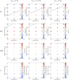 |
Fig. 14 Ion fractions of O I (top), O II (second row), and O III (third row), and the ejecta temperature Tej (bottom) in the simulations at one year for a realistic composition at three different values of TPWN. The black contour denotes the regime of low ejecta mass and high engine luminosity in which runaway ionization can occur for both O I and O II. |
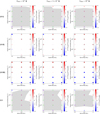 |
Fig. 15 Luminosity of the model [O I] (top), [O II] (second row), [O III] (third row), and O I (bottom) lines in units of the observed line luminosities and limits of SN 2012au at one year for the realistic composition at three different values of TPWN. The green circled points represent where the model and observed values are within a factor of two, the purple circles within a factor of five, and the gray shaded region also within a factor of five. The black circled points (for O I) represent where the model luminosity is more than a factor of two higher than the observational limit. The grid includes luminosity from all elements in the wavelength regions in which these lines are emitted. |
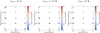 |
Fig. 16 Goodness-of-fit score for each model in the realistic composition at one year based on the [O I] and O I lines. Lower scores indicate a better fit to the data (from Eq. (12), a perfect fit has score 0, both lines off by a factor of two has a score of 0.18, and both lines off by a factor of ten has a score of 2). The black circles indicate the two models with the lowest scores for each TPWN, which are plotted in Fig. 17. |
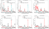 |
Fig. 17 Two best-fitting dust-corrected model spectra to SN 2012au for each value of TPWN at one years for the realistic composition compared to the observed spectrum from Milisavljevic et al. (2013). The total model emission is shown in red, and the emission from only oxygen is shown in cyan. Strong lines and features are labeled in the upper left plot. |
6 Discussion
6.1 Implications for initial conditions, the PWN spectrum, and the radio counterpart
One interesting possibility for nebular spectral modeling of magnetar-driven SNe is to combine with and cross-check other models to verify the inferred parameters or predict multiwave-length signals. The most common way to infer magnetar and ejecta parameters is with Bayesian inference on photometric data using light-curve models (e.g., Nicholl et al. 2017; Villar et al. 2018; Chen et al. 2023). Modeling early light curves can be done quickly on large samples and is sensitive to the magnetar spin period, which nebular spectra are not (Eq. (5)), as well as to magnetic field and ejecta mass. It is not sensitive to the PWN SED, however, which we have shown is important for understanding nebular spectra.
We used the two best-fit models from the pure oxygen composition at six years, 6O-4-2e39-1e5 and 6O-1.5-1e39-1e6, to show how these results might be combined with other methods. Figure 20 shows light curves generated using the model from Kashiyama et al. (2016) with spin periods of P0 = 1, 5, 10, and 15 ms and B and Mej given by the models and Eq. (5) compared to V-band photometric data from SN 2012au (Milisavljevic et al. 2013). The initial dipolar magnetic fields for these two models are 3 × 10¹⁴ G for the 6O-4-2e39-1e5 model and 4 × 10¹⁴ G for the 6O-1.5-1e39-1e6 model. Around the light-curve peak, the best-fit light curve has P0 = 15 ms, B = 4 × 10¹⁴ G, and Mej = 1.5 M⊙. This model has a spin-down time of 4.3 days, which is shorter than the rise time of the model, and a total rotational energy of 1.1 × 1050 erg, which is lower than a typical CCSN explosion energy of 1051 erg. These parameters are similar to those found by Pandey et al. (2021), although with a lower ejecta mass.
The injection SED temperature of 106 K from the 6O-1.5-1e39-1e6 model can be used to infer the electron injection Lorentz factor γb by assuming that the peak of the model black-body distribution corresponds to vb in Eq. (6). Assuming єB = 3 × 10⁻³, as was done for previous Galactic PWN models (Tanaka & Takahara 2010, 2013), γb = 3 × 10⁵ for this model, similar to the 105−106 inferred for Galactic PWNe. A value of єB ~ 10−6, similar to that inferred for SN 2015bn by Vurm & Metzger (2021), would only increase γb by a factor ~10, leaving it only slightly higher than that of Galactic PWNe.
When we assume spectral indices of q1 = 1.5 and q2 = 2.5 for a nebula with total power (Murase et al. 2015, 2021)
 (15)
(15)
as was done in Omand et al. (2018), Law et al. (2019), and Eftekhari et al. (2021), these parameters can be used to estimate radio emission from the PWN and compare it with the observation from Stroh et al. (2021) at seven years post-explosion. Using the model presented in Murase et al. (2015, 2016), who calculated PWN emission by self-consistently calculating synchrotron emission and self-absorption, pair cascades, Compton and inverse Compton scattering, adiabatic cooling, and both internal and external attenuation by solving the Boltzmann equation for electron-positron pairs and photons in the PWN over all electron energies and photon frequencies, we calculated the expected radio spectra for SN 2012au at 5, 7, 10, and 15 yr post-explosion, which is shown alongside the observed data in Fig. 21. This model predicts bright, long-lasting emission with a free-free absorption break that decreases in frequency with time. This emission is roughly consistent with observations and should easily be detectable by instruments such as the VLA for several decades.
The low-energy break in the spectra is caused by free-free absorption, which has an optical depth of
 (16)
(16)
where Te is the electron temperature, ne and ni are the electron and ion number densities, respectively, and  is the effective charge of the ejecta. This is normally estimated by assuming that the ejecta is 100% O II with Te = 104 (e.g., Omand et al. 2018; Law et al. 2019), but the nebular spectral model at six years shows that the ejecta has an electron fraction of ~0.8 and an electron temperature of ~6000 K, which we assumed are constant in time for these models and used in our calculation. These values are likely still uncertain due to model systematics, but using them to calculate absorption causes the break frequency to increase by about a factor of two with respect to the simple ejecta assumptions, with a small decrease in peak luminosity. This effect should become more pronounced at very late times, so the interpretation of radio SLSNe, such as PTF10hgi (Eftekhari et al. 2019, 2021; Mondal et al. 2020; Hatsukade et al. 2021), need to account for these deviations, and future models will have to constrain these values more strongly to be able to make predictions and aid future observational studies. Figure 21 also shows that these more detailed calculations are necessary for consistency with the previously observed data for SN 2012au (Stroh et al. 2021).
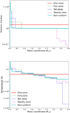 |
Fig. 18 Electron fraction (top) and ejecta temperature (bottom) for the multizone 1O-4-1e42-1e5 models. Only the nonuniform model can resolve the highly ionized inner ejecta region that is close to the PWN. |
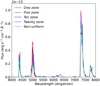 |
Fig. 19 Spectra for the multizone 10-4-1e42-1e5 models. The resolution of the ejecta can change line luminosities by up to a factor of about two if the ionization fraction of the emitting ion is strongly influenced by the resolution of the ejecta. |
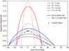 |
Fig. 20 Light-curve models for different spin periods with ejecta masses and magnetic fields derived from the 6O-4-2e39-1e5 and 6O-1.5-1e39-1e6 models, compared with V-band photometric data of SN 2012au from Milisavljevic et al. (2013). The most consistent model has a spin period P0 of 15 ms, and its parameters were derived from the 6O-1.5-1e39-1e6 model. |
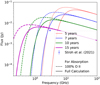 |
Fig. 21 Predicted radio spectra for SN 2012au at 5, 7, 10, and 15 yr post-explosion using the model determined by nebular spectral and light curve modeling, as well as the observed data at seven years from Stroh et al. (2021). The free-free absorption was calculated by assuming a completely singly ionized ejecta and electron temperature of 104, as was done in previous works, as well as using the output of our nebular spectral calculations. |
6.2 Mixing and clumping
It is very important to determine the extent of mixing in SN 2012au to properly model the nebular spectra. The results with the realistic composition showed that many models predicted strong optical calcium and sulphur lines, which were either barely detectable or undetectable. The fully mixed model we used here is the most extreme case of mixing and is likely unphysical (e.g., Jerkstrand 2017). Mixing in magnetar-driven SNe is mostly caused by Rayleigh-Taylor instabilities from the pulsar wind pushing on the ejecta, which will disrupt the initial shell structure and cause some mixing between regions. In simulations involving SLSN-like parameters, this usually creates two main zones: an outer region with mostly carbon and oxygen, and an inner region consisting of heavier elements (Chen et al. 2020; Suzuki & Maeda 2021). With more Ic-BL-like parameters (faster energy injection), these two zones will mix radially, but still be in different angular zones, meaning that creating an angle-averaged profile will miss the zonal separation (macroscopic versus microscopic mixing). The extent of mixing within each zone will depend on the characteristic size of the Rayleigh-Taylor instabilities, and will likely cause small regions within each zone that will retain the shell composition. However, for a less energetic magnetar, such as the P = 15 ms one inferred through light-curve modeling in Sect. 6.1, Rayleigh-Taylor instabilities may not develop on a large scale, and the shell structure of the progenitor may be mostly retained (see Fig. 5 from Suzuki & Maeda 2021, e.g.). By assuming Ic-BL-like mixing for this study instead of a shell structure consistent with a less energetic magnetar, we may have severely overestimated the extent of mixing in the ejecta: the generally unsatisfactory fits of our fully mixed models to SN 2012au strengthens the argument that complete microscopic mixing does not occur.
Understanding clumping of the ejecta (variation in densities over small or intermediate length scales in the ejecta), particularly in the inner regions that are most affected by hydro-dynamic instabilities, is also necessary to properly model the ejecta. Numerical simulations of SNe with strong central engines show that the unburnt C/O ashes reside in mostly high-density clumps, while the heavier elements reside in lower-density gas (Suzuki & Maeda 2021). Pandey et al. (2021) also reported a high imaging polarization value that is indicative of ejecta asymmetry. Jerkstrand et al. (2017) found that a strongly clumped O/Mg zone with a filling factor of ≲0.01 was needed to reproduce the nebular spectrum of SN 2015bn, and Dessart (2019) found that clumping is essential to trigger ejecta recombination and produce O I, Ca II, and Fe II lines, and that reproducing most SLSNe-I nebular spectra requires clumping. The multizone models from Sect. 5.3 show that resolving the high-density inner region is important for understanding the ionization structure of the ejecta and can affect line luminosities by a factor of a few. Modeling this region with a low filling factor will allow photons to reach further without being absorbed, but they will be less able to penetrate the clumps, leading to possible small-scale variations in the ionization structure of these clumps. This might have a large affect on the modeled spectrum and should be investigated in future studies.
Deciding how to model these effects will be important for more detailed models. The extent of these mixing and clumping effects largely depends on both the magnetar rotational energy and spin-down time, which both depend on the initial magnetar spin period. The nebular spectrum cannot directly probe this. Parameter estimation using the early light curve can help with this, but models of magnetar-driven SNe are generally not reliable for highly kinetic SNe due to the physical coupling between pulsar luminosity and ejecta kinetic energy. This is not included in some models (e.g., Nicholl et al. 2017). Adapting models for magnetar-driven kilonovae (Yu et al. 2013; Metzger 2019; Sarin et al. 2022) might be a viable strategy because the physics of these systems is largely similar. Inferred parameters from these models would allow both a qualitative characterization of multidimensionality in the SN and restrict the possible parameter space needed for nebular spectral synthesis calculations.
7 Summary
We presented a suite of late-time (1–6 yr) spectral simulations of SN ejecta powered by an inner PWN. To achieve this, we implemented an improved treatment of photoionization of key elements in the spectral synthesis code SUMO and extended the code to allow arbitrary radiative energy injection at an inner boundary.
Over a large grid of one-zone models, we studied the behavior of the physical state of the SN and of the line emission as PWN luminosity (LPWN), injection SED temperature (TPWN), ejecta mass (Mej), and composition (pure O or realistic) vary. We discussed the resulting emission in the context of the observed behavior of SN 2012au, a strong candidate for a PWN-powered SN.
We found that the oxygen ionization and ejecta temperature generally increase as the ejecta mass decreases and engine luminosity increases. The temperature range is about 1600-6300 K for pure oxygen models at six years, 400–6300 K for mixed composition models at six years, and ~4000–15 000 K for models with both compositions at one year. The dominant ion can be O I, O II or O III, depending on the combination of engine luminosity and ejecta mass.
Low ejecta mass models, at high PWN power, obtain runaway ionization (Jerkstrand et al. 2017) for O I, and in extreme cases, also O II, causing a sharp decrease in their ion fraction over a small change in the parameter space, and quenching of [O I] λλ 6300, 6364 (and [O II] λλ 7320, 7325). As the characteristic photon energy of the PWN SED increases, the ejecta becomes less ionized due to the lower number of ionizing photons. However, the ejecta temperature increases as the characteristic photon energy of the PWN SED increases.
Several pure oxygen models are able to reproduce the observed features of SN 2012au at six years (which shows strong [O I], [O II] and [O III] emission) to within a factor of about two. These models have LPWN ~ (1–5) × 1039 erg s−1 and Mej ~ 1.5–6 M⊙. As TPWN increases, the best-fit models have lower Mej and LPWN.
At one year, pure oxygen models with high TPWN have over-luminous [O II], [O III], and [O I] λ 5577 emission compared to observations, but models with lower TPWN can reproduce the oxygen features reasonably well. However, these models have a lower ejecta mass than at six years, a lower engine luminosity than would be expected for vacuum dipole spin down, and a lower injection SED temperature than would be expected for the typical evolution of a PWN SED (see Eq. (6)). These best-fit parameters are likely unphysical.
Realistic Ibc mixed composition models at six years require a stronger engine luminosity than in the pure oxygen models to reproduce the same oxygen line luminosities. These models cool strongly through IR radiation, particularly the [Ne II] 12.8 μm line, and have lower temperatures. Some models also exhibit strong [Ca II] and [S III] features in the optical band. We find no satisfactory simultaneous fit for O, Ca, and S lines to SN 2012au, which indicates that a fully mixed ejecta is not suitable.
Realistic Ibc mixed composition models at one year show strong [O II]/[Ca II] and [O III] emission over most of the parameter space. Only models with a low engine luminosity and low injection SED temperature are able to somewhat reproduce the spectrum, similar to the pure oxygen models. The realistic models tended to reproduce the observed oxygen/calcium lines more accurately over a larger parameter space than the pure oxygen models, but improved treatment of inner shell processes and mixing/clumping will be needed to reproduce all the spectral features with a high degree of accuracy.
Multizone models show that in 1D stratification, gradients develop both for ionization and temperature, with the innermost ejecta being the most highly ionized and hottest. Oxygen line luminosities can vary by a factor of a few depending on the stratification, which provides useful information about to which level of agreement one-zone models can be assessed against observations.
We demonstrated that results and constraints from nebular modeling can be connected into modeling of the diffusion phase and the radio emission. Light curves consistent with the best-fitting pure oxygen nebular spectral models at six years give an initial magnetar spin period of ~15 ms, and radio spectra predicted from these parameters have fluxes of ~10 mJy at ten years post explosion with a slow decline rate, meaning the remnant should be detectable for decades. These predictions are consistent with previous observations.
Future observations and modeling of SN 2012au and similar SNe could help test if the magnetar luminosity evolution is truly consistent with vacuum dipole spin-down and quantify the diversity in the PWN spectra associated with newborn millisecond magnetars. Improvements to the models could allow us to determine properties of these magnetars from the ever-increasing sample of SLSN nebular spectra, leading to a revolution in our understanding of these enigmatic neutron stars.
Acknowledgements
The authors would like to thank the anonymous referee for their helpful comments. The authors would also like to thank Akihiro Suzuki, Dan Milisavljevic, Mike Barlow, Maria Niculescu-Duvaz, Claes Fransson, Eliot Ayache, Bart van Baal, and Quentin Pognan for their helpful discussions. This project has received funding from the European Research Council (ERC) under the European Union’s Horizon 2020 Research and Innovation Programme (ERC Starting Grant No. [803189], PI: A. Jerkstrand). The computations were enabled by resources provided by the Swedish National Infrastructure for Computing (SNIC) at the PDC Center for High Performance Computing, KTH Royal Institute of Technology, partially funded by the Swedish Research Council through grant agreement no. 2018-05973.
Appendix A Code updates
Appendix A.1 Photon injection from the inner boundary
A module external to SUMO was developed that can generate a PWN spectrum to be used as an input to SUMO. This model can currently support blackbody spectra (with free parameters Ltot and TPWN), power-law spectra (with free parameters Ltot and q, the spectral index), and broken power-law spectra (with free parameters Ltot, λbreak, q1, and q2). The user also defines the wavelength resolution (which does not have to match the wavelength resolution of SUMO) and the minimum and maximum wavelengths. The user is also free to generate their own spectrum from external programs because the spectrum data files feature only one line with the number of bins and total luminosity, followed by two columns specifying the wavelength λ in angstrom and the spectral luminosities Lλ in erg s−1 cm−1.
To run a SUMO simulation using a central engine, the user needs to turn on the central engine flag in the runfile and to specify the filename for the engine spectrum. SUMO will then interpolate over that spectrum to create photon packets that are injected at the inner boundary of the innermost zone. These packets then propagate through the ejecta using the normal Monte Carlo routine.
Appendix A.2 Atomic data updates
The recombination rate and photoionization cross sections for some ions in the atomic data set used by SUMO had to be updated for this study. We added or updated the recombination rates of 16 ions to the dataset because they had never been relevant in previous simulations or because of the higher temperatures that are sometimes encountered in the solutions for engine-driven SNe. The list of ions with added or updated recombination rates and the source from which the rates were taken is given in Table A.1.
The photoinoization cross sections of all 13 ions with excited states with an energy lower than 2.72 eV (0.20 Ry) above the ground state (except for Fe, which had a cutoff of 1.36 eV) were updated. This cutoff was chosen because any higher energy states will be < 5% filled in thermal equilibrium at 10 000 K. Fe II was the only ion with multiple excited states below this cutoff. The cross sections σ were fit with multiple functions of the form
 (A.1)
(A.1)
where Eγ is the photon energy, Ei is the ionization energy, and σo and β are free parameters. Since a single power law does not fit the full cross section for any ion, the cross section was fit over different energy regimes using different power laws, with the regimes transitioning at λcut. Lists of the ions we updated and of fit parameters are given in Tables A.2 and A.3, and the fits are shown in Figure A.1.
By using power-law fits, we ignored the rapid variations in the cross sections that can occur due to resonances. In a homologously expanding ejecta, isotropic Doppler shifting smears the internal specific intensity out over frequency, and therefore, this treatment is expected to be acceptable.
Ions with updated total recombination rates.
Fitted parameters for the updated photoionization cross sections from highest to lowest energy. The fits are shown in Figure A.1.
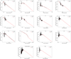 |
Fig. A.1 Updated fits for the photoionization cross sections from the first excited state of 13 ions (and second excited state for Fe II). Parameters for the fits are listed in Table A.3. |
References
- Anand, S., Barnes, J., Yang, S., et al. 2023, ApJ, submitted, [arXiv:2302.09226] [Google Scholar]
- Angus, C. R., Levan, A. J., Perley, D. A., et al. 2016, MNRAS, 458, 84 [NASA ADS] [CrossRef] [Google Scholar]
- Barkat, Z., Rakavy, G., & Sack, N. 1967, Phys. Rev. Lett., 18, 379 [Google Scholar]
- Barnes, J., & Metzger, B. D. 2022, ApJ, 939, L29 [NASA ADS] [CrossRef] [Google Scholar]
- Bautista, M. A. 1997, A&AS, 122, 167 [NASA ADS] [CrossRef] [EDP Sciences] [Google Scholar]
- Berger, E., Kulkarni, S. R., & Chevalier, R. A. 2002, ApJ, 577, L5 [NASA ADS] [CrossRef] [Google Scholar]
- Blanchard, P. K., Nicholl, M., Berger, E., et al. 2019, ApJ, 872, 90 [NASA ADS] [CrossRef] [Google Scholar]
- Blanchard, P. K., Berger, E., Nicholl, M., et al. 2021, ApJ, 921, 64 [NASA ADS] [CrossRef] [Google Scholar]
- Bode, M. F., & Evans, A. 1980, MNRAS, 193, 21 [NASA ADS] [Google Scholar]
- Cano, Z., Wang, S.-Q., Dai, Z.-G., et al. 2017, Adv. Astron, 2017, 8929054 [CrossRef] [Google Scholar]
- Chatzopoulos, E., Wheeler, J. C., & Vinko, J. 2012, ApJ, 746, 121 [Google Scholar]
- Chen, K.-J., Woosley, S. E., & Whalen, D. J. 2020, ApJ, 893, 99 [NASA ADS] [CrossRef] [Google Scholar]
- Chen, T. W., Smartt, S. J., Jerkstrand, A., et al. 2015, MNRAS, 452, 1567 [NASA ADS] [CrossRef] [Google Scholar]
- Chen, T. W., Brennan, S. J., Wesson, R., et al. 2021, ArXiv e-prints [arXiv:2109.07942] [Google Scholar]
- Chen, Z. H., Yan, L., Kangas, T., et al. 2023, ApJ, 943, 42 [NASA ADS] [CrossRef] [Google Scholar]
- Chevalier, R. A., & Fransson, C. 1992, ApJ, 395, 540 [NASA ADS] [CrossRef] [Google Scholar]
- Chevalier, R. A., & Fransson, C. 1994, ApJ, 420, 268 [NASA ADS] [CrossRef] [Google Scholar]
- Chugai, N. N., & Chevalier, R. A. 2006, ApJ, 641, 1051 [NASA ADS] [CrossRef] [Google Scholar]
- Chugai, N. N., Andronova, A. A., & Utrobin, V. P. 1996, Astron. Lett., 22, 672 [NASA ADS] [Google Scholar]
- Coppejans, D. L., Margutti, R., Guidorzi, C., et al. 2018, ApJ, 856, 56 [NASA ADS] [CrossRef] [Google Scholar]
- Corsi, A., Ho, A. Y. Q., Cenko, S. B., et al. 2022, AAS, submitted, [arXiv:2210.09536] [Google Scholar]
- Cunto, W., & Mendoza, C. 1992, Rev. Mexicana Astron. Astrofis., 23, 107 [Google Scholar]
- Dessart, L. 2018, A&A, 610, L10 [NASA ADS] [CrossRef] [EDP Sciences] [Google Scholar]
- Dessart, L. 2019, A&A, 621, A141 [NASA ADS] [CrossRef] [EDP Sciences] [Google Scholar]
- Dessart, L., Hillier, D. J., Waldman, R., et al. 2012, MNRAS, 426, L76 [NASA ADS] [CrossRef] [Google Scholar]
- Dessart, L., Waldman, R., Livne, E., et al. 2013, MNRAS, 428, 3227 [NASA ADS] [CrossRef] [Google Scholar]
- Dexter, J., & Kasen, D. 2013, ApJ, 772, 30 [NASA ADS] [CrossRef] [Google Scholar]
- Dwek, E. 1983, ApJ, 274, 175 [NASA ADS] [CrossRef] [Google Scholar]
- Eftekhari, T., Berger, E., Margalit, B., et al. 2019, ApJ, 876, L10 [NASA ADS] [CrossRef] [Google Scholar]
- Eftekhari, T., Margalit, B., Omand, C. M. B., et al. 2021, ApJ, 912, 21 [NASA ADS] [CrossRef] [Google Scholar]
- Filippenko, A. V., Matheson, T., & Ho, L. C. 1993, ApJ, 415, L103 [NASA ADS] [CrossRef] [Google Scholar]
- Fox, O. D., Chevalier, R. A., Dwek, E., et al. 2010, ApJ, 725, 1768 [NASA ADS] [CrossRef] [Google Scholar]
- Fransson, C., & Chevalier, R. A. 1989, ApJ, 343, 323 [NASA ADS] [CrossRef] [Google Scholar]
- Gal-Yam, A. 2012, Science, 337, 927 [Google Scholar]
- Gal-Yam, A., Mazzali, P., Ofek, E. O., et al. 2009, Nature, 462, 624 [NASA ADS] [CrossRef] [Google Scholar]
- Gendre, B., Stratta, G., Atteia, J. L., et al. 2013, ApJ, 766, 30 [Google Scholar]
- Ginzburg, S., & Balberg, S. 2012, ApJ, 757, 178 [NASA ADS] [CrossRef] [Google Scholar]
- Hatsukade, B., Tominaga, N., Morokuma, T., et al. 2021, ApJ, 911, L1 [NASA ADS] [CrossRef] [Google Scholar]
- Heger, A., & Woosley, S. E. 2002, ApJ, 567, 532 [Google Scholar]
- Howerton, S., Drake, A. J., Djorgovski, S. G., et al. 2012, Central Bureau Electronic Telegrams, 3052, 1 [NASA ADS] [Google Scholar]
- Inserra, C., Smartt, S. J., Jerkstrand, A., et al. 2013, ApJ, 770, 128 [NASA ADS] [CrossRef] [Google Scholar]
- Inserra, C., Bulla, M., Sim, S. A., et al. 2016, ApJ, 831, 79 [NASA ADS] [CrossRef] [Google Scholar]
- Ioka, K., Hotokezaka, K., & Piran, T. 2016, ApJ, 833, 110 [Google Scholar]
- Iwamoto, K., Mazzali, P. A., Nomoto, K., et al. 1998, Nature, 395, 672 [Google Scholar]
- Jerkstrand, A. 2017, in Handbook of Supernovae, eds. A. W. Alsabti, & P. Murdin (Berlin: Springer), 795 [CrossRef] [Google Scholar]
- Jerkstrand, A., Fransson, C., & Kozma, C. 2011, A&A, 530, A45 [NASA ADS] [CrossRef] [EDP Sciences] [Google Scholar]
- Jerkstrand, A., Fransson, C., Maguire, K., et al. 2012, A&A, 546, A28 [NASA ADS] [CrossRef] [EDP Sciences] [Google Scholar]
- Jerkstrand, A., Smartt, S. J., & Heger, A. 2016, MNRAS, 455, 3207 [NASA ADS] [CrossRef] [Google Scholar]
- Jerkstrand, A., Smartt, S. J., Inserra, C., et al. 2017, ApJ, 835, 13 [Google Scholar]
- Kamble, A., Soderberg, A. M., Chomiuk, L., et al. 2014, ApJ, 797, 2 [NASA ADS] [CrossRef] [Google Scholar]
- Kasen, D., & Bildsten, L. 2010, ApJ, 717, 245 [NASA ADS] [CrossRef] [Google Scholar]
- Kashiyama, K., Murase, K., & Bartos, I., 2016, ApJ, 818, 94 [NASA ADS] [CrossRef] [Google Scholar]
- Kennel, C. F., & Coroniti, F. V. 1984, ApJ, 283, 710 [Google Scholar]
- Kulkarni, S. R., Frail, D. A., Wieringa, M. H., et al. 1998, Nature, 395, 663 [NASA ADS] [CrossRef] [Google Scholar]
- Lasky, P. D., Leris, C., Rowlinson, A., et al. 2017, ApJ, 843, L1 [NASA ADS] [CrossRef] [Google Scholar]
- Law, C. J., Omand, C. M. B., Kashiyama, K., et al. 2019, ApJ, 886, 24 [NASA ADS] [CrossRef] [Google Scholar]
- Lee, C.-H. 2019, ApJ, 875, 121 [NASA ADS] [CrossRef] [Google Scholar]
- Lee, C.-H. 2020, Astron. Nachr., 341, 651 [NASA ADS] [CrossRef] [Google Scholar]
- Leloudas, G., Patat, F., Maund, J. R., et al. 2015a, ApJ, 815, L10 [NASA ADS] [CrossRef] [Google Scholar]
- Leloudas, G., Schulze, S., Krühler, T., et al. 2015b, MNRAS, 449, 917 [NASA ADS] [CrossRef] [Google Scholar]
- Levan, A. J., Tanvir, N. R., Starling, R. L. C., et al. 2014, ApJ, 781, 13 [Google Scholar]
- Li, Z.-Y., & Chevalier, R. A. 1999, ApJ, 526, 716 [NASA ADS] [CrossRef] [Google Scholar]
- Liljegren, S., Jerkstrand, A., & Grumer, J. 2020, A&A, 642, A135 [EDP Sciences] [Google Scholar]
- Liljegren, S., Jerkstrand, A., Barklem, P. S., et al. 2022, A&A submitted [arXiv:2203.07021] [NASA ADS] [CrossRef] [EDP Sciences] [Google Scholar]
- Lunnan, R., Chornock, R., Berger, E., et al. 2014, ApJ, 787, 138 [NASA ADS] [CrossRef] [Google Scholar]
- Lunnan, R., Chornock, R., Berger, E., et al. 2016, ApJ, 831, 144 [NASA ADS] [CrossRef] [Google Scholar]
- Lunnan, R., Fransson, C., Vreeswijk, P. M., et al. 2018, Nat. Astron., 2, 887 [NASA ADS] [CrossRef] [Google Scholar]
- Margalit, B., Metzger, B. D., Thompson, T. A., et al. 2018, MNRAS, 475, 2659 [NASA ADS] [CrossRef] [Google Scholar]
- Margutti, R., Chornock, R., Metzger, B. D., et al. 2018, ApJ, 864, 45 [NASA ADS] [CrossRef] [Google Scholar]
- Matheson, T., Filippenko, A. V., Li, W., et al. 2001, AJ, 121, 1648 [NASA ADS] [CrossRef] [Google Scholar]
- Mauerhan, J. C., Filippenko, A. V., Zheng, W., et al. 2018, MNRAS, 478, 5050 [NASA ADS] [CrossRef] [Google Scholar]
- Mazzali, P. A., Nomoto, K., Patat, F., et al. 2001, ApJ, 559, 1047 [NASA ADS] [CrossRef] [Google Scholar]
- Mazzali, P. A., Deng, J., Maeda, K., et al. 2002, ApJ, 572, L61 [NASA ADS] [CrossRef] [Google Scholar]
- Menzies, J. W., Catchpole, R. M., van Vuuren, G., et al. 1987, MNRAS, 227, 39 [NASA ADS] [Google Scholar]
- Metzger, B. D. 2019, Liv. Rev. Relativ., 23, 1 [NASA ADS] [Google Scholar]
- Metzger, B. D., Vurm, I., Hascoët, R., et al. 2014, MNRAS, 437, 703 [NASA ADS] [CrossRef] [Google Scholar]
- Metzger, B. D., Margalit, B., Kasen, D., et al. 2015, MNRAS, 454, 3311 [NASA ADS] [CrossRef] [Google Scholar]
- Milisavljevic, D., Fesen, R. A., Chevalier, R. A., et al. 2012, ApJ, 751, 25 [NASA ADS] [CrossRef] [Google Scholar]
- Milisavljevic, D., Soderberg, A. M., Margutti, R., et al. 2013, ApJ, 770, L38 [NASA ADS] [CrossRef] [Google Scholar]
- Milisavljevic, D., Margutti, R., Kamble, A., et al. 2015, ApJ, 815, 120 [NASA ADS] [CrossRef] [Google Scholar]
- Milisavljevic, D., Patnaude, D. J., Chevalier, R. A., et al. 2018, ApJ, 864, L36 [NASA ADS] [CrossRef] [Google Scholar]
- Mondal, S., Bera, A., Chandra, P., et al. 2020, MNRAS, 498, 3863 [NASA ADS] [CrossRef] [Google Scholar]
- Moriya, T. J., Nicholl, M., & Guillochon, J. 2018, ApJ, 867, 113 [NASA ADS] [CrossRef] [Google Scholar]
- Murase, K., Kashiyama, K., Kiuchi, K., et al. 2015, ApJ, 805, 82 [NASA ADS] [CrossRef] [Google Scholar]
- Murase, K., Kashiyama, K., & Mészáros, P. 2016, MNRAS, 461, 1498 [NASA ADS] [CrossRef] [Google Scholar]
- Murase, K., Omand, C. M. B., Coppejans, D. L., et al. 2021, MNRAS, 508, 44 [NASA ADS] [CrossRef] [Google Scholar]
- Nahar, S. N. 1995, ApJS, 101, 423 [NASA ADS] [CrossRef] [Google Scholar]
- Nahar, S. N. 1996a, ApJS, 106, 213 [NASA ADS] [CrossRef] [Google Scholar]
- Nahar, S. N. 1996b, Phys. Rev. A, 53, 1545 [NASA ADS] [CrossRef] [Google Scholar]
- Nahar, S. N. 1996c, Phys. Rev. A, 53, 2417 [NASA ADS] [CrossRef] [Google Scholar]
- Nahar, S. N. 1997, Phys. Rev. A, 55, 1980 [NASA ADS] [CrossRef] [Google Scholar]
- Nahar, S. N. 1998, Phys. Rev. A, 58, 3766 [Google Scholar]
- Nahar, S. N. 1999, ApJS, 120, 131 [NASA ADS] [CrossRef] [Google Scholar]
- Nahar, S. N. 2000, ApJS, 126, 537 [NASA ADS] [CrossRef] [Google Scholar]
- Nahar, S. N., & Pradhan, A. K. 1991, Phys. Rev. A, 44, 2935 [Google Scholar]
- Nahar, S. N., & Pradhan, A. K. 1993, J. Phys. B Atm. Mol. Phys., 26, 1109 [NASA ADS] [CrossRef] [Google Scholar]
- Nahar, S. N., & Pradhan, A. K. 1994a, J. Phys. B Atm. Mol. Phys., 27, 429 [NASA ADS] [CrossRef] [Google Scholar]
- Nahar, S. N., & Pradhan, A. K. 1994b, Phys. Rev. A, 49, 1816 [CrossRef] [Google Scholar]
- Nahar, S. N., & Pradhan, A. K. 1997, ApJS, 111, 339 [NASA ADS] [CrossRef] [Google Scholar]
- Nahar, S. N., Bautista, M. A., & Pradhan, A. K. 1997, ApJ, 479, 497 [NASA ADS] [CrossRef] [Google Scholar]
- Nahar, S. N., Bautista, M. A., & Pradhan, A. K. 1998, Phys. Rev. A, 58, 4593 [NASA ADS] [CrossRef] [Google Scholar]
- Nahar, S. N., Pradhan, A. K., & Zhang, H. L. 2000, ApJS, 131, 375 [NASA ADS] [CrossRef] [Google Scholar]
- Nakauchi, D., Kashiyama, K., Suwa, Y., et al. 2013, ApJ, 778, 67 [NASA ADS] [CrossRef] [Google Scholar]
- Nicholl, M. 2021, Astron. Geophys., 62, 5.34 [CrossRef] [Google Scholar]
- Nicholl, M., Smartt, S. J., Jerkstrand, A., et al. 2013, Nature, 502, 346 [NASA ADS] [CrossRef] [Google Scholar]
- Nicholl, M., Berger, E., Margutti, R., et al. 2016, ApJ, 828, L18 [NASA ADS] [CrossRef] [Google Scholar]
- Nicholl, M., Guillochon, J., & Berger, E. 2017, ApJ, 850, 55 [NASA ADS] [CrossRef] [Google Scholar]
- Nicholl, M., Blanchard, P. K., Berger, E., et al. 2018, ApJ, 866, L24 [NASA ADS] [CrossRef] [Google Scholar]
- Nicholl, M., Berger, E., Blanchard, P. K., et al. 2019, ApJ, 871, 102 [NASA ADS] [CrossRef] [Google Scholar]
- Niculescu-Duvaz, M., Barlow, M. J., Bevan, A., et al. 2022, MNRAS, 515, 4302 [NASA ADS] [CrossRef] [Google Scholar]
- Omand, C. M. B., Kashiyama, K., & Murase, K. 2018, MNRAS, 474, 573 [NASA ADS] [CrossRef] [Google Scholar]
- Omand, C. M. B., Kashiyama, K., & Murase, K. 2019, MNRAS, 484, 5468 [NASA ADS] [CrossRef] [Google Scholar]
- Ørum, S. V., Ivens, D. L., Strandberg, P., et al. 2020, A&A, 643, A47 [NASA ADS] [CrossRef] [EDP Sciences] [Google Scholar]
- Pandey, S. B., Kumar, A., Kumar, B., et al. 2021, MNRAS, 507, 1229 [NASA ADS] [CrossRef] [Google Scholar]
- Parthasarathy, A., Johnston, S., Shannon, R. M., et al. 2020, MNRAS, 494, 2012 [NASA ADS] [CrossRef] [Google Scholar]
- Pastorello, A., Smartt, S. J., Botticella, M. T., et al. 2010, ApJ, 724, L16 [NASA ADS] [CrossRef] [Google Scholar]
- Pognan, Q., Jerkstrand, A., & Grumer, J. 2022a, MNRAS, 513, 5174 [NASA ADS] [CrossRef] [Google Scholar]
- Pognan, Q., Jerkstrand, A., & Grumer, J. 2022b, MNRAS, 510, 3806 [NASA ADS] [CrossRef] [Google Scholar]
- Poidevin, F., Omand, C. M. B., Pérez-Fournon, I., et al. 2022, MNRAS, 511, 5948 [NASA ADS] [CrossRef] [Google Scholar]
- Poidevin, F., Omand, C. M. B., Könyves-Tóth, R., et al. 2023, MNRAS, 521, 5418 [NASA ADS] [CrossRef] [Google Scholar]
- Pursiainen, M., Leloudas, G., Paraskeva, E., et al. 2022, A&A, 666, A30 [NASA ADS] [CrossRef] [EDP Sciences] [Google Scholar]
- Quimby, R. M., De Cia, A., Gal-Yam, A., et al. 2018, ApJ, 855, 2 [Google Scholar]
- Saito, S., Tanaka, M., Moriya, T. J., et al. 2020, ApJ, 894, 154 [NASA ADS] [CrossRef] [Google Scholar]
- Sarangi, A., Dwek, E., & Arendt, R. G. 2018, ApJ, 859, 66 [NASA ADS] [CrossRef] [Google Scholar]
- Sarin, N., Omand, C. M. B., Margalit, B., et al. 2022, MNRAS, 516, 4949 [Google Scholar]
- Şaşmaz Muş, S., Çikinloǧlu, S., Aygün, U., et al. 2019, ApJ, 886, 5 [CrossRef] [Google Scholar]
- Schulze, S., Krühler, T., Leloudas, G., et al. 2018, MNRAS, 473, 1258 [NASA ADS] [CrossRef] [Google Scholar]
- Smith, N., Foley, R. J., & Filippenko, A. V. 2008, ApJ, 680, 568 [Google Scholar]
- Soderberg, A. M., Berger, E., Page, K. L., et al. 2008, Nature, 453, 469 [NASA ADS] [CrossRef] [Google Scholar]
- Stroh, M. C., Terreran, G., Coppejans, D. L., et al. 2021, ApJ, 923, L24 [NASA ADS] [CrossRef] [Google Scholar]
- Sun, L., Xiao, L., & Li, G. 2022, MNRAS, 513, 4057 [NASA ADS] [CrossRef] [Google Scholar]
- Suzuki, A., & Maeda, K. 2017, MNRAS, 466, 2633 [NASA ADS] [CrossRef] [Google Scholar]
- Suzuki, A., & Maeda, K. 2019, ApJ, 880, 150 [NASA ADS] [CrossRef] [Google Scholar]
- Suzuki, A., & Maeda, K. 2021, ApJ, 908, 217 [NASA ADS] [CrossRef] [Google Scholar]
- Taddia, F., Sollerman, J., Fremling, C., et al. 2019, A&A, 621, A71 [NASA ADS] [CrossRef] [EDP Sciences] [Google Scholar]
- Takaki, K., Kawabata, K. S., Yamanaka, M., et al. 2013, ApJ, 772, L17 [NASA ADS] [CrossRef] [Google Scholar]
- Tanaka, S. J., & Takahara, F. 2010, ApJ, 715, 1248 [NASA ADS] [CrossRef] [Google Scholar]
- Tanaka, S. J., & Takahara, F. 2013, MNRAS, 429, 2945 [CrossRef] [Google Scholar]
- Taubenberger, S., Valenti, S., Benetti, S., et al. 2009, MNRAS, 397, 677 [NASA ADS] [CrossRef] [Google Scholar]
- Villar, V. A., Nicholl, M., & Berger, E. 2018, ApJ, 869, 166 [NASA ADS] [CrossRef] [Google Scholar]
- Vurm, I., & Metzger, B. D. 2021, ApJ, 917, 77 [NASA ADS] [CrossRef] [Google Scholar]
- West, S. L., Lunnan, R., Omand, C. M. B., et al. 2023, A&A, 670, A7 [NASA ADS] [CrossRef] [EDP Sciences] [Google Scholar]
- Woosley, S. E. 2010, ApJ, 719, L204 [NASA ADS] [CrossRef] [Google Scholar]
- Woosley, S. E., & Heger, A. 2007, Phys. Rep., 442, 269 [Google Scholar]
- Yan, L., Quimby, R., Ofek, E., et al. 2015, ApJ, 814, 108 [NASA ADS] [CrossRef] [Google Scholar]
- Yan, L., Lunnan, R., Perley, D. A., et al. 2017, ApJ, 848, 6 [NASA ADS] [CrossRef] [Google Scholar]
- Yu, Y.-W., Zhang, B., & Gao, H. 2013, ApJ, 776, L40 [CrossRef] [Google Scholar]
All Tables
Values of dλ1 for each line and epoch used to determine the observed and model line luminosities.
Fitted parameters for the updated photoionization cross sections from highest to lowest energy. The fits are shown in Figure A.1.
All Figures
|
Fig. 1 Schematic showing the dependence of the third line-luminosity factor on ne, A, and ϒ. Lines with the same A values (red and green) will approach the same luminosity in the high ne (LTE) limit, lines with the same ϒ values (blue and red) show the same luminosity in the low ne limit, and lines with the same A/ϒ (blue and green) show the same value of ncrit, while ncrit for the red line is a factor of x larger. |
| In the text | |
|
Fig. 2 Ion fractions of O I (top), O II (second row), and O III (third row), and the ejecta temperature Tej (bottom) in the simulations at six years for a pure oxygen composition at three different values of TPWN. The black contour denotes the regime with a low ejecta mass and high engine luminosity in which runaway ionization can occur for both O I and O II. |
| In the text | |
|
Fig. 3 Luminosity of the model [O I] (top), [O II] (second row), [O III] (third row), and O I (bottom) lines in units of the observed line luminosities and limits for SN 2012au at six years for a pure oxygen composition at three different values of TPWN. The green circled points represent where the model and observed values are within a factor of 2, the purple circles within a factor of 5, and the gray shaded region also within a factor of 5 for clarity. For O I (bottom panel), the black circled points represent where the model luminosity is more than a factor 2 higher than the observational upper limit. |
| In the text | |
|
Fig. 4 Goodness-of-fit score for each model for the pure oxygen composition at six years based on the [O I], [O II], and [O III] lines. Lower scores indicate a better fit to the data (from Eq. (12), a perfect fit has a score of 0, all three lines off by a factor of two has a score of 0.27, and all three lines off by a factor of ten has a score of 3). The black circles indicate the two models with the lowest scores for each TPWN, which are plotted in Fig. 5. |
| In the text | |
|
Fig. 5 Two best-fitting dust-corrected model spectra to SN 2012au for each value of TPWN at six years for a pure oxygen composition compared to the observed spectrum from Milisavljevic et al. (2018). Strong lines and features are labeled in the upper left plot. |
| In the text | |
|
Fig. 6 Ion fractions of O I (top), O II (second row), and O III (third row), and the ejecta temperature Tej (bottom) in the simulations at one year for a pure oxygen composition at three different values of TPWN. The black contour denotes the regime with low ejecta mass and high engine luminosity in which runaway ionization can occur for both O I and O II. |
| In the text | |
|
Fig. 7 Luminosity of the model [O I] (top), [O II] (second row), [O III] (third row), and O I (bottom) lines in units of the observed line luminosities and limits for SN 2012au at one year for a pure oxygen composition at three different values of TPWN. The green circled points represent where the model and observed values are within a factor of 2, the purple circles within a factor of 5, and the gray shaded region also within a factor of 5. The black circled points (for [O II] and [O III]) represent where the model luminosity is more than a factor of two higher than the observational limit. |
| In the text | |
|
Fig. 8 Goodness-of-fit score for each model for the pure oxygen composition at one year based on the [O I] and O I lines. Lower scores indicate a better fit to the data (from Eq. (12), a perfect fit has a score of 0, both lines off by a factor of two has a score of 0.18, and both lines off by a factor of ten has score 2). The black circles indicate the two models with the lowest scores for each TPWN, which are plotted in Fig. 9. |
| In the text | |
|
Fig. 9 Two best-fitting dust-corrected model spectra to SN 2012au for each value of TPWN at one year for a pure oxygen composition compared to the observed spectrum from Milisavljevic et al. (2013). Strong lines and features are labeled in the upper left plot. |
| In the text | |
|
Fig. 10 Ion fractions of O I (top), O II (second row), and O III (third row), and the ejecta temperature Tej (bottom) in the simulations at six years for the realistic composition at three different values of TPWN. The black contour denotes the regime of low ejecta mass and high engine luminosity in which runaway ionization can occur for both O I and O II. |
| In the text | |
|
Fig. 11 Luminosity of the model [O I] (top), [O II] (second row), [O III] (third row), and O I (bottom) lines compared to the observed line luminosities and luminosity limits from SN 2012au at six years for the realistic composition at three different values of TPWN. The green circled points represent where the model and observed values are within a factor of 2two, the purple circles within a factor of five, and the gray shaded region also within a factor of five. The black circled points represent where the model luminosity is more than a factor of two higher than the observational limit. The grid includes luminosity from all elements in the wavelength regions in which these lines are emitted. |
| In the text | |
|
Fig. 12 Goodness-of-fit score for each model in the realistic composition at six years based on the [O I], [O II], and [O III] lines. Lower scores indicate a better fit to the data (from Eq. (12), a perfect fit has a score of 0, all three lines off by a factor of two has a score of 0.27, and all three lines off by a factor of ten has a score of 3). The black circles indicate the two models with the lowest scores for each TPWN, although TPWN = 105 K has no models with scores <3, and TPWN = 3 × 10⁵ K has no models with scores <2. The best-fitting models for TPWN = 106 K are plotted in Fig. 13 |
| In the text | |
|
Fig. 13 Two best-fitting dust-corrected model spectra for TPWN = 106 K at six years for the realistic composition compared to the observed spectrum from Milisavljevic et al. (2018). The total model emission is shown in red, and the emission from only oxygen is shown in cyan. Strong lines and features are labeled in the left plot. |
| In the text | |
|
Fig. 14 Ion fractions of O I (top), O II (second row), and O III (third row), and the ejecta temperature Tej (bottom) in the simulations at one year for a realistic composition at three different values of TPWN. The black contour denotes the regime of low ejecta mass and high engine luminosity in which runaway ionization can occur for both O I and O II. |
| In the text | |
|
Fig. 15 Luminosity of the model [O I] (top), [O II] (second row), [O III] (third row), and O I (bottom) lines in units of the observed line luminosities and limits of SN 2012au at one year for the realistic composition at three different values of TPWN. The green circled points represent where the model and observed values are within a factor of two, the purple circles within a factor of five, and the gray shaded region also within a factor of five. The black circled points (for O I) represent where the model luminosity is more than a factor of two higher than the observational limit. The grid includes luminosity from all elements in the wavelength regions in which these lines are emitted. |
| In the text | |
|
Fig. 16 Goodness-of-fit score for each model in the realistic composition at one year based on the [O I] and O I lines. Lower scores indicate a better fit to the data (from Eq. (12), a perfect fit has score 0, both lines off by a factor of two has a score of 0.18, and both lines off by a factor of ten has a score of 2). The black circles indicate the two models with the lowest scores for each TPWN, which are plotted in Fig. 17. |
| In the text | |
|
Fig. 17 Two best-fitting dust-corrected model spectra to SN 2012au for each value of TPWN at one years for the realistic composition compared to the observed spectrum from Milisavljevic et al. (2013). The total model emission is shown in red, and the emission from only oxygen is shown in cyan. Strong lines and features are labeled in the upper left plot. |
| In the text | |
|
Fig. 18 Electron fraction (top) and ejecta temperature (bottom) for the multizone 1O-4-1e42-1e5 models. Only the nonuniform model can resolve the highly ionized inner ejecta region that is close to the PWN. |
| In the text | |
|
Fig. 19 Spectra for the multizone 10-4-1e42-1e5 models. The resolution of the ejecta can change line luminosities by up to a factor of about two if the ionization fraction of the emitting ion is strongly influenced by the resolution of the ejecta. |
| In the text | |
|
Fig. 20 Light-curve models for different spin periods with ejecta masses and magnetic fields derived from the 6O-4-2e39-1e5 and 6O-1.5-1e39-1e6 models, compared with V-band photometric data of SN 2012au from Milisavljevic et al. (2013). The most consistent model has a spin period P0 of 15 ms, and its parameters were derived from the 6O-1.5-1e39-1e6 model. |
| In the text | |
|
Fig. 21 Predicted radio spectra for SN 2012au at 5, 7, 10, and 15 yr post-explosion using the model determined by nebular spectral and light curve modeling, as well as the observed data at seven years from Stroh et al. (2021). The free-free absorption was calculated by assuming a completely singly ionized ejecta and electron temperature of 104, as was done in previous works, as well as using the output of our nebular spectral calculations. |
| In the text | |
|
Fig. A.1 Updated fits for the photoionization cross sections from the first excited state of 13 ions (and second excited state for Fe II). Parameters for the fits are listed in Table A.3. |
| In the text | |
Current usage metrics show cumulative count of Article Views (full-text article views including HTML views, PDF and ePub downloads, according to the available data) and Abstracts Views on Vision4Press platform.
Data correspond to usage on the plateform after 2015. The current usage metrics is available 48-96 hours after online publication and is updated daily on week days.
Initial download of the metrics may take a while.