| Issue |
A&A
Volume 671, March 2023
|
|
|---|---|---|
| Article Number | A87 | |
| Number of page(s) | 10 | |
| Section | The Sun and the Heliosphere | |
| DOI | https://doi.org/10.1051/0004-6361/202244997 | |
| Published online | 09 March 2023 | |
No evidence for synchronization of the solar cycle by a “clock”
1
Brunnenstr. 58, 61231 Bad Nauheim, Germany
2
Max-Planck-Institut für Sonnensystemforschung, Justus-von-Liebig-Weg 3, 37077 Göttingen, Germany
e-mail: cameron@mps.mpg.de
Received:
16
September
2022
Accepted:
7
January
2023
The length of the solar activity cycle fluctuates considerably. The temporal evolution of the corresponding cycle phase, that is, the deviation of the epochs of activity minima or maxima from strict periodicity, provides relevant information concerning the physical mechanism underlying the cyclic magnetic activity. An underlying strictly periodic process (akin to a perfect “clock”), with the observer seeing a superposition of the perfect clock and a small random phase perturbation, leads to long-term phase stability in the observations. Such behavior would be expected if cycles were synchronized by tides caused by orbiting planets or by a hypothetical torsional oscillation in the solar radiative interior. Alternatively, in the absence of such synchronization, phase fluctuations accumulate and a random walk of the phase ensues, which is a typical property of randomly perturbed dynamo models. Based on the sunspot record and the reconstruction of solar cycles from cosmogenic 14C, we carried out rigorous statistical tests in order to decipher whether there exists phase synchronization or random walk. Synchronization is rejected at significance levels of between 95% (28 cycles from sunspot data) and beyond 99% (84 cycles reconstructed from 14C), while the existence of random walk in the phases is consistent with all data sets. This result strongly supports randomly perturbed dynamo models with little inter-cycle memory.
Key words: Sun: activity / Sun: general / methods: statistical / dynamo
© The Authors 2023
 Open Access article, published by EDP Sciences, under the terms of the Creative Commons Attribution License (https://creativecommons.org/licenses/by/4.0), which permits unrestricted use, distribution, and reproduction in any medium, provided the original work is properly cited.
This article is published in open access under the Subscribe to Open model.
Open access funding provided by Max Planck Society.
1. Introduction
The historical sunspot record reveals significant variability in the amplitude and length of the individual activity cycles. In order to understand the physical mechanism underlying the variable cyclic activity, it is important to answer the question of whether the phase of the activity cycle shows long-term stability. In this case, although the length of the individual cycles fluctuates, the cycle appears to remain synchronized to some strictly periodic process (akin to a “clock”). This means that the fluctuations of the cycle length do not correspond to real phase changes but reflect, for instance, observational errors or varying transit times of magnetic flux rising through the convection zone. Such a situation would occur if the activity cycles were triggered, for example, by a hypothetical high-Q torsional oscillation in the solar interior (Dicke et al. 1970) or by minuscule tidal forces exerted by the planets (e.g., Stefani et al. 2021). Alternatively, in the absence of such synchronization in the system, phase fluctuations can lead to a random walk of the phase. This would happen in the case of a cyclic dynamo with a period that varies because of random fluctuations of dynamo excitation or meridional flow. We note that the clock case could also correspond to a dynamo, albeit one with an externally enforced fixed period.
(Yule 1927) took an ideal pendulum as a simple mechanical example to illustrate both cases: if the motion of the pendulum is undisturbed, but the observation of its position is subject to measurement error, we have a case of phase stability and synchronization. Alternatively, if the pendulum were to be randomly bombarded with peas, the resulting phase fluctuations would accumulate and the phase would show a random walk.
There have been previous attempts in the literature to explore the phase stability of the solar cycle on the basis of empirical data. The sunspot record since 1700 provides a relatively consistent dataset, but has generally been considered to be too short for a reliable statistical phase analysis (e.g., Hoyng 1996). Further extension of the cycle into the past has been attempted on the basis of reports of pre-telescopic sightings of sunspots and aurorae. The problem there is that the sporadic and often ambiguous reports are much too sparse to faithfully determine the times of maxima and minima of individual cycles with yearly precision (e.g., Stephenson 1988, 1990). Nevertheless, Schove (1955, 1983) gave years of sunspot minima and maxima back to the year 649 B.C., mainly relying on aurora reports. However, as he imposed a fixed number of nine cycles per century, he assumed phase stability beforehand (Nataf 2022), meaning that these data are useless for our purposes. Catalogs of naked-eye observations of sunspots in the pre-telescopic era (Wittmann 1978; Wittmann & Xu 1987) are even more sparse and show no clustering around the maxima of a hypothetical phase-stable cycle (Stix 1983, 1984). Furthermore, Carrasco et al. (2020) compared naked-eye observations with telescopic records in the 19th century and found that the naked-eye observations do not necessarily correspond to high solar activity or large sunspot groups, meaning that such observations cannot be used offhandedly to infer the timing of individual cycle maxima (see also Usoskin et al. 2015). Similar arguments apply to historical reports considered to represent aurorae, although long-term activity variations and grand minima may tentatively be identified in these data. A comprehensive and critical summary of the use of historical documents to infer solar phenomena in the past was given by Vaquero & Vázquez (2009).
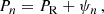
Although claims of phase stability of the solar cycle can be found in various papers (e.g., Lomb 2013; Russell et al. 2019; Stefani et al. 2020), a conclusive answer to the question of phase stability or otherwise requires both a clear definition of phase stability and proper statistical analysis. For instance, nonmonotonic evolution of phase in the sense that sequences of positive excursions of phase over a number of cycles are seemingly “compensated for” by later cycles (e.g., Charbonneau & Dikpati 2000) does not necessarily entail phase stability, synchronization, or memory (see examples in Fig. 1). This refers also, for instance, to the well-known weak anti-correlation between cycle length and amplitude (Hoyng 1996; Lomb 2013).
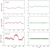 |
Fig. 1. Examples of Monte Carlo simulations of the phase evolution for case R (random walk, left panels) and for case C (synchronization, right panels) and different numbers of cycles. |
The first systematic statistical studies of the phase stability of the solar cycle were presented by Dicke (1978) and Gough (1978), who carried out conceptually similar analyses based on the telescopic sunspot record. Both authors concluded that the available data were not sufficient to decisively discriminate between random walk and phase synchronization. Subsequently, Gough (1981, 1983, 1988) corrected and modified his earlier analysis, still concluding that the results do not permit the rejection of one of the alternatives.
In this paper, we revisit the problem using the additional cycle maximum and minimum epochs until 2019 (28 cycles compared to 24 cycles available in 1981) as well as the reconstruction of 84 solar cycles between the years 976 and 1888 based on a new analysis of 14C in tree rings (Brehm et al. 2021; Usoskin et al. 2021). Extending the analyses of Gough (1981, 1983), we find that these data are statistically consistent with random walk of the cycle phase and exclude clock synchronization with at high levels of significance.
The paper is organized as follows. In Sect. 2 we consider the disparate phase evolution of a randomly perturbed, memory-less oscillator (random walk of phase) and of a perturbed clock-synchronized system and reconsider the statistical method of Gough (1981, 1983), thereby correcting an error in his original analysis. We apply the method to the up-to-date sunspot record and to the 14C-based reconstruction in Sect. 3. Further tests concerning the significance of the results are presented in Sect. 4. Section 5 contains our conclusions.
2. Random walk of phase versus synchronization: statistical analysis
2.1. The method of Gough (1981)
Following Gough (1981), we consider two extreme cases as the basis of our statistical analysis. The first case corresponds to the absence of inter-cycle memory: stochastic fluctuations of cycle length lead to random walk of phase. The alternative case is a perturbed cyclic system whose period is fixed through synchronization by a perfect clock: any fluctuation in the timing of cycle number n does not affect the timing of cycle n + 1. For convenience, we call the first model random walk (in short: case R) and the second model clock (in short: case C).
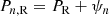
We consider epochs of the cycle minima (or maxima), tn (n = 0, …N). In both cases (R and C), we have random fluctuations of the cycle length, for example due to its dependence on fluctuating parameters (case R) or to time delays of the transfer of magnetic flux through the turbulent convection zone (case C). In case C, the resulting phase fluctuations do not accumulate, because the governing periodic process runs with a fixed period and phase, meaning that previous fluctuations appear to be “corrected” by synchronization, and we have
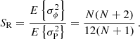
where PC is the clock period and τn is the (random) phase fluctuation in cycle n. In contrast, for case R, the phase fluctuations, ψi, accumulate, so that
where PR is the period at which the undisturbed system would operate in the absence of fluctations. In practice, both PC and PR correspond to the average of the cycle length over an infinite set of cycles, so that, in principle, they could have been denoted by the same symbol. For clarity, we continue to use separate symbols in what follows. These two simple models confer an advantage in that they are quite general and independent of the detailed nature of the phase changes (e.g., discrete random jumps or more gradual variations during the cycle). Of course, more explicit models could be analyzed more deeply and therefore possibly yield more detailed results.
We illustrate the disparate phase evolution for both cases using a simple example. We assume PR = PC = 11 yr and normally distributed phase fluctuations with zero mean and a standard deviation of 2 yr. Figure 1 shows the evolution of the phases for both cases (τn and ∑ψi, respectively) and for different total numbers of cycles (note the different scaling of the ordinate axes). The two cases are virtually indistinguishable if only ten periods are considered. With 84 cycles, which is the length of the reconstructed sunspot record by Usoskin et al. (2021), differences are visible and finally become obvious for 1024 cycles. We note that random walk of phase does not imply that the phase evolves monotonically; indeed in our case of a probability distribution for phase fluctuations that is symmetric with respect to zero, a random walk corresponds to a recurrent Markov chain that returns to zero infinitely often. Such returns have therefore nothing to do with any kind of “clock correction of phase deviations”. The random walk with 1024 cycles clearly shows such returns as well as intervals with approximately linear phase drift, which, if viewed in isolation, could easily be mistaken as evidence for phase stability with respect to a matching period.
In the case of the solar cycle, available datasets are not sufficiently long to decide the case simply by visual inspection of the phase evolution: a proper statistical analysis needs to be carried out. Here, we follow the approach of Gough (1981, 1983), which is sketched below (an example of the detailed calculations is given in the Appendix).
We have a series of epochs of cycle minima (or maxima), tn (n = 0, …N), covering N cycles. The aim of the analysis is to define statistical criteria that allow us to decide whether these data are consistent with (or exclude) the clock case (C, synchronization) or random phase walk (case R) as given in Eqs. (1) and (2). The observed period of cycle n, Pn = tn − tn − 1, is given by
for case C and by
for case R. As the “true” periods, PC and PR, are not known from the data, they are estimated by the mean period over the N empirical cycles, ⟨P⟩=(tN − t0)/N, meaning that we have
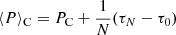
for case C and
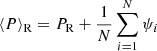
for case R. The phase deviations with respect to the mean period are generally defined as

meaning that we obtain

for case C, and
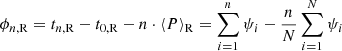
for case R. In both cases, we therefore start with zero phase deviation for n = 0.
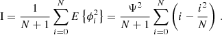
The basis for the statistical analysis are the expectation values of the variances of cycle period and phase deviation, namely
for the period and
for the phase deviations, where the angular brackets indicate the arithmetic mean. For both cases, we assume uncorrelated phase fluctuations (τi and ψi, respectively) with zero mean. A somewhat lengthy, but straightforward calculation (see appendix) yields the expectation values of the variances as functions of the number of cycles (N) and the amplitudes of the fluctuations (𝒯2 and Ψ2, respectively). For the expectation value of the variance of period, we obtain
for case C and
for case R, both in agreement with Gough (1981). The expectation value of the variance of phase for case C is given by
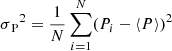
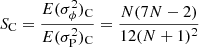
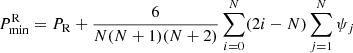
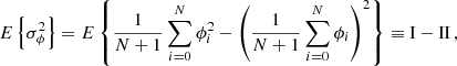
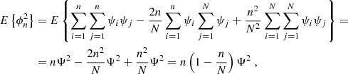
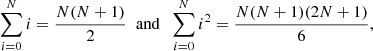
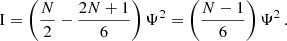
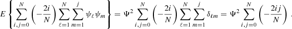
![$$ \begin{aligned} E(\sigma _\phi ^2)_{\mathrm{C} }&= E\left({1\over N+1}\sum _{i=0}^N\phi _i^2\right) - E\left(\left[{1\over N+1}\sum _{i=0}^N\phi _i \right]^2\right) \nonumber \\&= {5N^2-6N+1\over 3N(N+1)}\mathcal{T} ^2 - {(N-1)\over 2(N+1)}\mathcal{T} ^2 \nonumber \\&= {(7N-2)(N-1)\over 6N(N+1)}\mathcal{T} ^2 . \end{aligned} $$](/articles/aa/full_html/2023/03/aa44997-22/aa44997-22-eq14.gif)
Here, Gough (1981) apparently omitted the second term on the r.h.s. of Eq. (11), meaning that our result differs from his. Likewise, for case R, we obtain

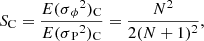
The final statistic is defined as the ratio of the variances, meaning that the unknown fluctuation amplitudes cancel out. The result is
for case C and
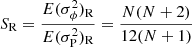
for case R. For large values of N, SC approaches a constant value of 7/12, while SR approaches linear growth corresponding to N/12. This is half of the slope obtained by Gough (1981). We cross-checked the correctness of our analytical calculations using Monte Carlo simulations.
2.2. Modified method (Gough 1983)
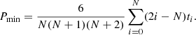
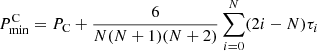
In follow-up papers, Gough (1983, 1988) modified his analysis, referring to Dicke (1978). Instead of taking the arithmetic mean of the cycle periods provided by the data as in Eqs. (5) and (6), an estimate of the “true” periods, PC or PR, is determined by minimizing the variance of phase deviation,  . The phases are generally given by ϕn = tn − t0 − nP and Pmin is determined by the minimalization process, as
The resulting periods for the two cases are then given by
for case C, and
for case R. Clearly, for growing values of N, these expressions converge more rapidly to the “true” periods than the estimates derived from the average period given by Eqs. (5) and (6).
Based on these period estimates, the corresponding ratios of expectation values for the variances of phase deviation and period are given by
for case C and
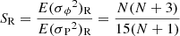
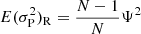
for case R, both in agreement with the expressions given by Gough (1983).
3. Application to observed and reconstructed sunspot cycles
We consider a set of empirical epochs of solar cycle minima (or maxima), tn (n = 0…M), corresponding to M cycles. The individual periods are then Pi = ti − ti − 1 (i = 1…M) and the phase deviations with respect to the estimate, Pest, of the “true” period are determined as ϕn = tn − t0 − n ⋅ Pest (n = 0…M). Pest is calculated either as the arithmetic mean of the individual periods (original Gough method) or by minimalization of  (modified method).
The full data set of M cycles is divided into contiguous segments of N(q) = M/q cycles each, where the values of q are the divisors of M. For each q, the mean variances,  and
and  , are determined according to Eqs. (10) and (11) as averages over the corresponding segments of length N(q). The ratio
  is then plotted as a function of N(q), to be compared with the curves corresponding to the ratio of the analytically calculated expectation values, SC and SR.
Confidence intervals with regard to SC and SR are determined by Monte Carlo simulations. We assume normally distributed phase fluctuations τn and ψn, respectively, with zero mean and a standard deviation of 2 yr to compute 10 000 realizations of M perturbed 11 yr cycles for each of the two cases according to Eqs. (1) and (2). The assumed standard deviation is consistent with the value inferred for 84 solar cycles reconstructed from 14C by Usoskin et al. (2021), but the precise choice is irrelevant, as the statistic S neither depends on the amplitude nor on the standard deviation of the distribution of the phase fluctuations. Following the procedures described in the previous section, we then calculate the values of S for each value of N(q) and for all realizations. From the resulting distributions of SC and SR, we determine the one-sided 68%, 95%, and 99% percentiles: as the distributions are generally not symmetric, we start from the average value and separately count the number of realizations until we reach the given percentile on each side. For a normal distribution, these percentiles would (approximately) correspond to the ±1σ, ±2σ, and ±3σ ranges, where σ denotes the standard deviation.
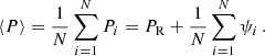
As a first application, we consider the telescopic sunspot record. Gough (1981, 1983), considered the maximum and minimum epochs of 24 cycles between the years 1712 and 1976. Using the epochs provided by the SILSO database1, we redid his analysis using both the (corrected) original method and the modified method as presented in Sect. 2. The results are shown in Fig. 2. Already with the 24 cycles available to Gough (1981), the data points for both variants of the method align well with the blue line representing the expectation values for case R. Clock synchronization (case C) can be rejected at the 95% confidence level. Owing to its better convergence property, the modified method provides somewhat narrower confidence intervals than the original method. The differences between the diagram in the left panel of Figs. 2 and 7 of Gough (1981) result from the correction of the calculation of the variance of phase (see Sect. 2). This leads to a downward shift of the theoretical curves for both cases. The result is that even the limited data available in the early 1980s clearly favor case R, that is, a random walk of the phase of the solar cycle. This is in accordance with the results presented in Gough (1983, 1988).
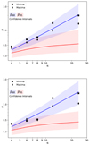 |
Fig. 2. Application of the statistical methods of Gough (1981, 1983) to the epochs of sunspot minima and maxima of 24 activity cycles between 1712 and 1976. Upper panel: (Corrected) Original method of Gough (1981). Lower panel: modified method (Gough 1983). In both panels, the symbols show the ratio |


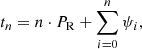
In the meantime, data for 28 cycles have become available. Figure 3 shows the results of the statistical analysis. The longer data series confirms and strengthens the results obtained on the basis of 24 cycles. In particular, the confidence intervals have become narrower compared to Fig. 2, meaning that the rejection of the synchronization hypothesis becomes even more significant.
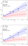 |
Fig. 3. Same as Fig. 2, now on the basis of the sunspot data for 28 solar cycles between 1712 and 2019. Compared to Fig. 2, the confidence intervals have become somewhat narrower, owing to the longer data set, thus strengthening the conclusion: clock synchronization is rejected at a confidence level of at least 95%, while random walk of phase is consistent with the data. |
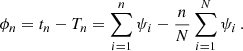
The recent reconstruction of 84 cycles (between the years 976 and 1888) on the basis of the cosmogenic isotope 14C by Usoskin et al. (2021) provides a significant extension of the database available for the analysis. Figure 4 shows the results of applying both variants of the Gough method to these data; they confirm and significantly reinforce the results drawn from the sunspot data: clock synchronization is now rejected at a confidence level of at least 99%, while random walk remains consistent with the data.
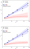 |
Fig. 4. Application of the statistical analysis to the series of 84 cycles covering the period between the years 976 and 1888 as reconstructed from 14C data by (Usoskin et al. 2021). Upper panel: (Corrected) Original method of Gough (1981). Lower panel: modified method (Gough 1983). The graphical representation of the results is the same as in the previous figures. The data are consistent with random walk of phase (case R) while, owing to the much longer data set, clock synchronization is rejected at levels exceeding 99%. |
The longer set of reconstructed cycles allows us to also consider the distribution of the phase deviations, ϕn, as a means to qualitatively discriminate between the cases C and R. The upper row of Fig. 5 shows the distribution of phase deviations for the 84 reconstructed cycles from the 14C record (relative to the mean period of 10.9 yr) in comparison to the corresponding distributions from one realization of the Monte Carlo simulations of 84 artificial cycles for case R and the same for case C. Both simulations assume a base period of 11 years with a standard deviation of 2.2 years for the phase fluctuations. As the phase deviations accumulate in case R (upper middle panel), the corresponding distribution is significantly broader (σ = 6.3 yr) than that of case C (upper right panel, σ = 2.2 yr), the latter reflecting the input Gaussian distribution. Likewise, the distribution for the 84 reconstructed cycles (upper left panel, σ = 6.2 yr) is also markedly broader than that of the simulated case C. For case R, we can retrieve the individual phase fluctuation, ψn, of cycle n as the difference ϕn − ϕn − 1. This is shown in the lower row of Fig. 5. For the simulated case R, the result (based on the mean period) therefore closely reflects the input distribution (lower middle panel). However, if we apply the same procedure to the simulated case C, this necessarily leads to a broader distribution than the input, because it results from the difference of two Gaussian distributions, τn − τn − 1 (lower right panel). We can therefore use this procedure as a qualitative method to distinguish whether a given dataset corresponds to case R or to case C: if the distribution of ϕn − ϕn − 1 is narrower than the original distribution, this indicates case R, while a broader distribution favors case C. The two panels corresponding to the 14C reconstructions on the left side of Fig. 5 clearly show that the reconstructed solar cycles behave as expected for case R, that is, the distribution of the inferred phase fluctuations for the individual cycles is significantly narrower (σ = 2.2 yr) than that of the original phase deviations (σ = 6.2 yr).
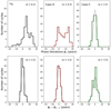 |
Fig. 5. Distributions of phase deviations (upper panels) and inferred phase fluctuations (differences between subsequent phase deviations, lower panels) for the 84 reconstructed cycles from the 14C data (left panels) and for simulated cycles with Gaussian fluctuations corresponding to case R (middle panels) and case C (right panels). The dotted curves indicate Gaussian fits. |
4. Further tests
4.1. Systematic effects
We consider two systematic effects that can influence the epochs of activity maxima and minima. Firstly, the “Waldmeier effect”, which is the correlation between the rise time from activity minimum to maximum and the amplitude of a cycle (Waldmeier 1935), affects the times of the maxima. This effect enhances the variance of the period determined from the maxima and possibly explains why the empirical S values corresponding to the set of cycle maxima tend to be somewhat lower than those for the minima (see Figs. 2–4). Following Dicke (1978), Gough (1981, 1983) corrected the sunspot data for the Waldmeier effect and found that the results were not significantly affected.
Secondly, activity cycles overlap, that is, flux emergence of a new cycle already starts at mid solar latitudes while the previous cycle is still present at low latitudes. In combination with the Waldmeier effect, this leads to an amplitude-dependent shift of the minimum epochs (Cameron & Schüssler 2007). Incidentally, this shift also explains the empirical statistical relationship between cycle length and amplitude. Hathaway et al. (1994) and Hathaway (2011) used curve fitting to an empirical standard cycle shape to obtain starting dates of sunspot cycles 1–23 (1755 until 1996) that are not affected by cycle overlap. The result of applying the modified Gough test (Sect. 2.2) to these data is given in Fig. 6. Comparison with the square symbols presented in Figs. 2b and 3b shows that the shift of the minimum epochs due to cycle overlap and the Waldmeier effect does not significantly affect the statistical results of the Gough test.
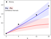 |
Fig. 6. Application of the modified method of Gough (1983) to the unbiased starting dates of solar cycles 1–23 determined by Hathaway et al. (1994) and Hathaway (2011). |
4.2. Dependence on the length of the data set
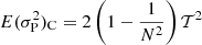
The length of the data set, that is, the number of observed cycles, is crucial for the capability of a statistical test to distinguish between case C and case R. Our results show that the set of 84 cycles reconstructed from the 14C record permits a much more stringent answer than the 28 cycles provided by the sunspot record. In order to systematically assess the reliability of the original and modified Gough methods, we used Monte Carlo simulations to determine the false-alarm probability (FAP) with respect to the 99% confidence interval as a function of the total number of cycles, M. For each given M, we computed 106 realizations of each of the models, that is, case C (Eq. (3)) and case R (Eq. (4)). For each realization, we calculated the value of our statistic, S, for N = M, which provides the largest difference between SR and SC, and is therefore the most sensitive. We then determined the FAPs, that is, the percentage of the realizations of case C with S values within the 99% confidence interval for case R and, conversely, the percentage of the realizations of case R with S values within the 99% confidence interval for case C.
The results of this procedure for both the original and the modified Gough test are shown in Fig. 7. The red curves correspond to the FAP for case R, meaning the probability that a realization of case R would fall within the 99% confidence interval of case C, or in other words the probability of misclassification as case C at that level. Likewise, the blue lines give the probability for misclassfying a realization of case C as case R. The figures clearly show that the modified method provides significantly lower values of the FAP, particularly for larger M. Reasonably low values of less than 1% FAP are reached for M > 50 for the original Gough test and M > 30 for the modified test. This corresponds to the results shown in Sect. 3: while the clock hypothesis can be safely rejected at the 99% significance level for M = 84 using the 14C-based data, this can only be done at 95% significance level for M = 24(28) on the basis of the sunspot record.
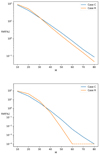 |
Fig. 7. False-alarm probabilities as a function of the total number of cycles in the data set, based on Monte Carlo simulations. Upper panel: (Corrected) Original method of Gough (1981). Lower panel: modified method (Gough 1983). The red lines give the FAP that a realization of case C falls within the 99% confidence interval for case R, and vice versa for the blue lines. The dashed line segment indicates an upper limit. |
4.3. The method of Eddington and Plakidis
A problem very similar to the question of phase stability of the solar cycle was considered by Eddington & Plakidis (1929). These authors considered the question of whether the brightness changes of long-period variable stars have an underlying fixed period with superposed observational errors (analogous to the clock case in the context of the present study) or if the individual periods vary randomly without memory (i.e., the random walk case). The authors considered the mean value,  , of the accumulated phase error after x epochs of maximum brightness with respect to the mean period over the whole length of the data set. Assuming that the period variations consist of a combination of accumulating (random walk) and nonaccumulating (clock-type) fluctuations, the expectation value is given by
where α is the amplitude of the synchronized fluctuations (e.g., measurement errors) and ϵ the amplitude of the cumulating fluctuations (leading to random walk of phase). A correction factor (in parentheses) is applied to account for the cases where x becomes a considerable fraction of the total number of periods, M, in the data set.  can be calculated from the data and a least-squares fit to Eq. (23) provides empirical values of the amplitudes α and ϵ, from which the relative importance of clock and random walk can be assessed.
We calculated  on the basis of the minimum epochs of the 84 activity cycles determined from the 14C data. The results and the fit to Eq. (23) are shown in Fig. 8. As the individual values of the accumulated phase, ux, are significantly affected by overlap for large values of x, we restricted the fit to x ≤ 50. The fit results in α < 10−4 yr for the amplitude of the nonaccumulating fluctuations and ϵ = 1.9 yr for the amplitude of the cumulating fluctuations. This clearly demonstrates that the system is nearly exclusively governed by random walk of the cycle phase, thus corroborating the results of the Gough test.
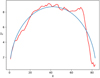 |
Fig. 8. Application of the test of Eddington & Plakidis (1929) to the 84 reconstructed cycles on the basis of the 14C data. Shown is the mean accumulated phase error after x cycles as a function of x. The red curve results from the activity minima of the reconstructed cycles, the blue curve is the corresponding fit to the theoretical relation given by Eq. (23) for x ≤ 50. The resulting fit parameters clearly indicate that the system shows random walk of phase. |
5. Conclusions
Using rigorous statistical tests, we investigated whether or not the phase of the solar cycle is stable, that is, whether it is synchronized by some kind of clock or follows a random walk. Our analysis is based on 28 activity cycles from the historical sunspot record and 84 cycles reconstructed from 14C data in tree rings. The tests reveal that these data unequivocally favor random walk of the cycle phase and exclude clock synchronization, with high significance levels (95% for sunspot data and greatly exceeding 99% for the 14C data). Consequently, data that unambiguously correspond to solar activity cycles provide no basis for the “planetary hypothesis” or for hypothetical high-Q oscillations in the radiative interior as drivers or “synchronizers” of the solar cycle. Likewise, data for an exoplanetary system also provide no evidence for planetary synchronization of stellar cycles (Obridko et al. 2022). The consistency of the phase evolution with random walk suggests that a randomly perturbed, memoryless dynamo action is the cause of the solar activity cycle (e.g., Charbonneau & Dikpati 2000; Cameron & Schüssler 2017; Karak & Miesch 2018).
Acknowledgments
Ilya Usoskin kindly provided the reconstructed sunspot numbers obtained by Usoskin et al. (2021) in electronic form. We are grateful to the referee for making us aware of the paper by Eddington & Plakidis (1929).
References
- Brehm, N., Bayliss, A., Christl, M., et al. 2021, Nat. Geosci., 14, 10 [Google Scholar]
- Cameron, R. H., & Schüssler, M. 2007, ApJ, 659, 801 [NASA ADS] [CrossRef] [Google Scholar]
- Cameron, R. H., & Schüssler, M. 2017, ApJ, 843, 111 [NASA ADS] [CrossRef] [Google Scholar]
- Carrasco, V. M. S., Gallego, M. C., Arlt, R., & Vaquero, J. M. 2020, ApJ, 904, 60 [NASA ADS] [CrossRef] [Google Scholar]
- Charbonneau, P., & Dikpati, M. 2000, ApJ, 543, 1027 [NASA ADS] [CrossRef] [Google Scholar]
- Dicke, R. H. 1970, in IAU Colloq. 4: Stellar Rotation, ed. A. Slettebak (Dordrecht: Reidel), 289 [CrossRef] [Google Scholar]
- Dicke, R. H. 1978, Nature, 276, 676 [NASA ADS] [CrossRef] [Google Scholar]
- Eddington, A. S., & Plakidis, S. 1929, MNRAS, 90, 65 [NASA ADS] [CrossRef] [Google Scholar]
- Gough, D. 1978, in Pleins Feux sur la Physique Solaire, eds. S. Roesch, & J. Dumont, 81 [Google Scholar]
- Gough, D. 1981, Variations of the Solar Constant (NASA Conference Publication) 2191, 185 [NASA ADS] [Google Scholar]
- Gough, D. O. 1983, ESA J., 7, 325 [NASA ADS] [Google Scholar]
- Gough, D. O. 1988, in Solar-Terrestrial Relationships and the Earth Environment in the Last Millennia, ed. G. Cini Castagnoli (Amsterdam: North-Holland), 90 [Google Scholar]
- Hathaway, D. H. 2011, Sol. Phys., 273, 221 [NASA ADS] [CrossRef] [Google Scholar]
- Hathaway, D. H., Wilson, R. M., & Reichmann, E. J. 1994, Sol. Phys., 151, 177 [NASA ADS] [CrossRef] [Google Scholar]
- Hoyng, P. 1996, Sol. Phys., 169, 253 [NASA ADS] [CrossRef] [Google Scholar]
- Karak, B. B., & Miesch, M. 2018, ApJ, 860, L26 [NASA ADS] [CrossRef] [Google Scholar]
- Lomb, N. 2013, J. Phys. Conf. Ser., 440, 012042 [CrossRef] [Google Scholar]
- Nataf, H.-C. 2022, Sol. Phys., 297, 107 [NASA ADS] [CrossRef] [Google Scholar]
- Obridko, V. N., Katsova, M. M., & Sokoloff, D. D. 2022, MNRAS, 516, 1251 [NASA ADS] [CrossRef] [Google Scholar]
- Russell, C. T., Jian, L. K., & Luhmann, J. G. 2019, Rev. Geophys., 57, 1129 [NASA ADS] [CrossRef] [Google Scholar]
- Schove, D. J. 1955, J. Geophys. Res., 60, 127 [NASA ADS] [CrossRef] [Google Scholar]
- Schove, D. J. 1983, in Sunspot Cycles (Hutchinson Ross Publ. Comp.), 68 [Google Scholar]
- Stefani, F., Beer, J., Giesecke, A., et al. 2020, Astron. Nachr., 341, 600 [NASA ADS] [CrossRef] [Google Scholar]
- Stefani, F., Stepanov, R., & Weier, T. 2021, Sol. Phys., 296, 88 [NASA ADS] [CrossRef] [Google Scholar]
- Stephenson, F. R. 1988, in Solar-Terrestrial Relationships and the Earth Environment in the last Millennia, ed. G. Cini Castagnoli (Amsterdam: North-Holland), 133 [Google Scholar]
- Stephenson, F. R. 1990, Phil. Transf. R. Soc. London, Ser. A, 330, 499 [CrossRef] [Google Scholar]
- Stix, M. 1983, Mitteilungen Astronomischen Gesellschaft Hamburg, 60, 95 [NASA ADS] [Google Scholar]
- Stix, M. 1984, Astron. Nachr., 305, 215 [NASA ADS] [CrossRef] [Google Scholar]
- Usoskin, I. G., Arlt, R., Asvestari, E., et al. 2015, A&A, 581, A95 [CrossRef] [EDP Sciences] [Google Scholar]
- Usoskin, I. G., Solanki, S. K., Krivova, N. A., et al. 2021, A&A, 649, A141 [NASA ADS] [CrossRef] [EDP Sciences] [Google Scholar]
- Vaquero, J. M., & Vázquez, M. 2009, in The Sun Recorded Through History (Berlin: Springer), 361 [CrossRef] [Google Scholar]
- Waldmeier, M. 1935, Astron. Mitteilungen Eidgenössischen Sternwarte Zürich, 14, 105 [Google Scholar]
- Wittmann, A. 1978, A&A, 66, 93 [NASA ADS] [Google Scholar]
- Wittmann, A. D., & Xu, Z. T. 1987, A&AS, 70, 83 [NASA ADS] [Google Scholar]
- Yule, G. U. 1927, Phil. Transf. R. Soc. London A, 226, 267 [NASA ADS] [CrossRef] [Google Scholar]
Appendix A: Calculation of the statistic SR
In what follows, we describe the calculation of the statistic  for case R (random walk of phase) as would be expected for a randomly perturbed dynamo. We follow Gough (1981) and write, for the nth observed period,
where PR is the “true” period (in the absence of fluctuations) and ψn denotes random, uncorrelated perturbations with zero mean and amplitude Ψ, namely

The unknown period PR is estimated via the arithmetic mean of the periods given by
For the expectation value of the variance of period, we obtain
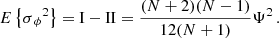
![$$ \begin{aligned} E\left\{ \sigma {_{\mathrm{P} }}^2\right\}&= E\left\{ {1\over N} \sum _{i=1}^N \left( P_i - \langle P \rangle \right)^2 \right\} = E\left\{ {1\over N} \sum _{i=1}^N \left(\psi _i - {1\over N} \sum _{j=1}^N \psi _j\right)^2\right\} = \nonumber \\&= E\left\{ {1\over N} \sum _{i=1}^N \left[ \psi _i^2 - {2\psi _i\over N}\sum _{j=1}^N \psi _j + {1\over N^2}\sum _{k=1}^N\sum _{\ell =1}^N \psi _k\psi _\ell \right]\right\} = \Psi ^2 - {2\Psi ^2\over N} + {\Psi ^2\over N} = {N-1\over N}\Psi ^2 \;. \end{aligned} $$](/articles/aa/full_html/2023/03/aa44997-22/aa44997-22-eq38.gif)
The phase deviations are defined by ϕn = tn − t0 − n ⋅ ⟨P⟩, where
and so we obtain
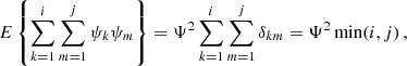
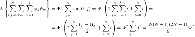
We now consider the expectation value of the variance of the phase deviation,
which consists of two terms (denoted by I and II). For calculating term I, we first consider
which leads to
With
we obtain
This agrees with the result given by Gough (1981) for the complete variance of the phase deviation. However, for the correct result, we must also consider the second term, II, in Eq. A.7, namely
![$$ \begin{aligned} \mathrm{II}&= E\left\{ \left({1\over N+1} \sum _{i=0}^N\phi _i \right)^2 \right\} = {1\over (N+1)^2} E\left\{ \sum _{i,j=0}^N \phi _i\phi _j \right\} = \nonumber \\&= {1\over (N+1)^2} E\left\{ \sum _{i,j=0}^N \left(\sum _{k=1}^i\psi _k-{i\over N}\sum _{\ell =1}^N\psi _\ell \right) \left( \sum _{m=1}^j\psi _m-{j\over N}\sum _{n=1}^N\psi _n\right)\right\} = \nonumber \\&= {1\over (N+1)^2} E\left\{ \sum _{i,j=0}^N \left[ \sum _{k=1}^i\sum _{m=1}^j\psi _k\psi _m + {ij\over N^2}\sum _{\ell =1}^N\sum _{n=1}^N\psi _\ell \psi _n - {2i\over N}\sum _{\ell =1}^N\sum _{m=1}^j\psi _\ell \psi _m \right]\right\} \,. \end{aligned} $$](/articles/aa/full_html/2023/03/aa44997-22/aa44997-22-eq46.gif)
We have
which means that for the first term in curly brackets in the bottom row of Eq. (A.12) we obtain
For the second term in curly brackets in the bottom row of Eq. (A.12), we find
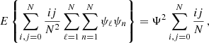
while the third term yields
This means that the sum of the second and the third term becomes
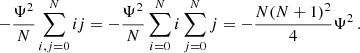
Adding the terms in Eqs. A.14 and A.17, we obtain
![$$ \begin{aligned} \mathrm{{II}} = E\left\{ \left({1\over N+1} \sum _{i=0}^N\phi _i \right)^2 \right\} = {1\over (N+1)^2} \left[ {N(N+1)(2N+1)\over 6} - {N(N+1)^2\over 4}\right] \Psi ^2 = {N(N-1)\over 12(N+1)} \Psi ^2 \,. \end{aligned} $$](/articles/aa/full_html/2023/03/aa44997-22/aa44997-22-eq52.gif)
Using Eqs. (A.11) and (A.18), the result for the variance of the phase deviation becomes
With Eq. A.4, we finally determine the statistic SR for the case of random phase walk, that is,
For N → ∞, SR behaves as N/12, in contrast to N/6 as given by Gough (1981).
All Figures
|
Fig. 1. Examples of Monte Carlo simulations of the phase evolution for case R (random walk, left panels) and for case C (synchronization, right panels) and different numbers of cycles. |
| In the text | |
|
Fig. 2. Application of the statistical methods of Gough (1981, 1983) to the epochs of sunspot minima and maxima of 24 activity cycles between 1712 and 1976. Upper panel: (Corrected) Original method of Gough (1981). Lower panel: modified method (Gough 1983). In both panels, the symbols show the ratio |
| In the text | |
|
Fig. 3. Same as Fig. 2, now on the basis of the sunspot data for 28 solar cycles between 1712 and 2019. Compared to Fig. 2, the confidence intervals have become somewhat narrower, owing to the longer data set, thus strengthening the conclusion: clock synchronization is rejected at a confidence level of at least 95%, while random walk of phase is consistent with the data. |
| In the text | |
|
Fig. 4. Application of the statistical analysis to the series of 84 cycles covering the period between the years 976 and 1888 as reconstructed from 14C data by (Usoskin et al. 2021). Upper panel: (Corrected) Original method of Gough (1981). Lower panel: modified method (Gough 1983). The graphical representation of the results is the same as in the previous figures. The data are consistent with random walk of phase (case R) while, owing to the much longer data set, clock synchronization is rejected at levels exceeding 99%. |
| In the text | |
|
Fig. 5. Distributions of phase deviations (upper panels) and inferred phase fluctuations (differences between subsequent phase deviations, lower panels) for the 84 reconstructed cycles from the 14C data (left panels) and for simulated cycles with Gaussian fluctuations corresponding to case R (middle panels) and case C (right panels). The dotted curves indicate Gaussian fits. |
| In the text | |
|
Fig. 6. Application of the modified method of Gough (1983) to the unbiased starting dates of solar cycles 1–23 determined by Hathaway et al. (1994) and Hathaway (2011). |
| In the text | |
|
Fig. 7. False-alarm probabilities as a function of the total number of cycles in the data set, based on Monte Carlo simulations. Upper panel: (Corrected) Original method of Gough (1981). Lower panel: modified method (Gough 1983). The red lines give the FAP that a realization of case C falls within the 99% confidence interval for case R, and vice versa for the blue lines. The dashed line segment indicates an upper limit. |
| In the text | |
|
Fig. 8. Application of the test of Eddington & Plakidis (1929) to the 84 reconstructed cycles on the basis of the 14C data. Shown is the mean accumulated phase error after x cycles as a function of x. The red curve results from the activity minima of the reconstructed cycles, the blue curve is the corresponding fit to the theoretical relation given by Eq. (23) for x ≤ 50. The resulting fit parameters clearly indicate that the system shows random walk of phase. |
| In the text | |
Current usage metrics show cumulative count of Article Views (full-text article views including HTML views, PDF and ePub downloads, according to the available data) and Abstracts Views on Vision4Press platform.
Data correspond to usage on the plateform after 2015. The current usage metrics is available 48-96 hours after online publication and is updated daily on week days.
Initial download of the metrics may take a while.