| Issue |
A&A
Volume 671, March 2023
|
|
|---|---|---|
| Article Number | A104 | |
| Number of page(s) | 11 | |
| Section | Extragalactic astronomy | |
| DOI | https://doi.org/10.1051/0004-6361/202244941 | |
| Published online | 09 March 2023 | |
Exploring extreme conditions for star formation: A deep search for molecular gas in the Leo ring
1
INAF-Osservatorio di Arcetri, Largo E. Fermi 5, 50125
Firenze, Italy
e-mail: This email address is being protected from spambots. You need JavaScript enabled to view it.
2
Department of Physics and Astronomy, The Johns Hopkins University, Baltimore, MD, 21210
USA
Received:
9
September
2022
Accepted:
6
December
2022
Abstract
Aims. We carried out sensitive searches for the 12CO J = 1–0 and J = 2–1 lines in the giant extragalactic HI ring in Leo to investigate the star formation process within environments where gas metallicities are close to solar, but physical conditions are different than those typical of bright galaxy disks. Our aim is to check the range of validity of known scaling relations.
Methods. We used the IRAM-30 m telescope to observe 11 regions close to HI gas peaks or where sparse young massive stars have been found. For all pointed observations we reached spectral noise between 1 and 5 mK for at least one of the observed frequencies at 2 km s−1 spectral resolution.
Results. We marginally detect two 12CO J = 1–0 lines in the star-forming region Clump 1 of the Leo ring, whose radial velocities are consistent with those of Hα lines, but whose line widths are much smaller than observed for virialized molecular clouds of similar mass in galaxies. The low signal-to-noise ratio, the small line widths, and the extremely low number densities inferred by virialized cloud models suggest that a more standard population of molecular clouds, still undetected, might be in place. Using upper limits to the CO lines, the most sensitive pointed observations show that the molecular gas mass surface density is lower than expected from the extrapolation of the molecular Kennicutt–Schmidt relation established in the disk of galaxies. The sparse stellar population in the ring, possibly forming ultra diffuse dwarf galaxies, might then be the result of a short molecular gas depletion time in this extreme environment.
Key words: galaxies: star formation / galaxies: dwarf / ISM: molecules / submillimeter: ISM / HII regions / galaxies: interactions
© The Authors 2023
 Open Access article, published by EDP Sciences, under the terms of the Creative Commons Attribution License (https://creativecommons.org/licenses/by/4.0), which permits unrestricted use, distribution, and reproduction in any medium, provided the original work is properly cited.
This article is published in open access under the Subscribe to Open model. This email address is being protected from spambots. You need JavaScript enabled to view it. to support open access publication.
1. Introduction
Although our understanding of the basic physical processes leading to star formation is based on high resolution Galactic studies (e.g., André et al. 2019), nearby galaxies have often complemented Milky Way studies offering a variety of interstellar medium (ISM) conditions to be examined (Corbelli et al. 2012, 2017; Leroy et al. 2013, 2021; Elmegreen 2015). Extragalactic surveys have widened our knowledge of the star formation process by inspecting how this changes as galaxies evolve through cosmic time, as galaxy mass, morphology, and metallicity change (e.g., Kennicutt & Evans 2012; Krumholz et al. 2012; Tacconi et al. 2020; Lutz et al. 2021). Dwarf galaxies and outer disks of spiral galaxies have been targets used to investigate star formation laws in low density regions (Thilker et al. 2007; Krumholz 2013; Elmegreen & Hunter 2015; Watson et al. 2016; López-Sánchez et al. 2018; Corbelli et al. 2019). Some key questions arise regarding the formation of the molecular phase and its tracers, as well as the scaling relation of the star formation rate (SFR) with the surface or volume gas density, such as the Kennicutt–Schmidt (K–S) law (Bigiel et al. 2010; Krumholz 2012; de los Reyes & Kennicutt 2019; Bacchini et al. 2020). The low metallicities, however, have often limited the interpretation of results, especially those concerning the formation and evolution of molecular clouds, building blocks of the star formation process and traced via CO lines (Bolatto et al. 2013; Hunt et al. 2015; Archer et al. 2022).
Very few studies have been dedicated to the formation of stars at yet another extreme: metal-rich low density regions, such as intergalactic neutral clouds of tidal origin. Most studied cases deal with shocked gas recently removed from the disk of galaxies through tidal encounters where the gas and star formation densities are high (Braine et al. 2000; Lisenfeld et al. 2004; Querejeta et al. 2021). The paucity of more quiescent cold clouds in the Local Universe, with only occasional formation of stars, surely limits the exploration of the slow star formation process in these metal-rich but low density environments. However, these clouds offer the unique opportunity to test star formation laws at extremely low rates where gas physical conditions are different than in disk galaxies (with no rotational support and no stellar disk driving supersonic turbulence). Stochasticity at the upper end of the stellar initial mass function (IMF) and density dependencies of the CO-to-H2 conversion factor (Lamers et al. 2002; da Silva et al. 2014; Hu et al. 2022) requires some caution in interpreting the results; nevertheless, understanding star formation in extragalactic clouds of tidal origin is very relevant because we might capture the slow build-up process of diffuse dwarf galaxy formation (Pasha et al. 2021).
The serendipitous discovery of an optically dark HI cloud in the M96 group (Schneider et al. 1983) has since triggered a great deal of discussion on the origin and survival of the most extended and massive HI structure in the local intergalactic medium. With an extension of about 200 kpc and a neutral gas mass MHI = 2 × 10⁹ M⊙, the cloud has a ring-like shape; it is also known as the Leo ring which might orbit the galaxies M 105 and NGC 3384 with a 4 Gyr period (Schneider 1985). The ring is more than three Holmberg radii distant from any known galaxy, and is significantly larger than other known collisional rings. The lack of a significant intragroup diffuse starlight and of an extended optical counterpart of the ring (Pierce & Tully 1985; Kibblewhite et al. 1985; Watkins et al. 2014) supports the ring primordial origin hypothesis (Schneider et al. 1989; Sil’chenko et al. 2003). Intermediate resolution HI maps, obtained with the Very Large Array (VLA) with an effective beam of 45″, revealed the presence of gas clumps (Schneider et al. 1986) with column densities of order 1021 cm−2 with a few of these associated with faint ultraviolet (UV) emitting regions, indicative of recent localized events of star formation (Thilker et al. 2009). Spectroscopic data, acquired recently for two major HI clumps in the Leo ring (Clump1 and Clump2E) have recently given new insights into the Leo cloud mystery, revealing the presence of ionized gas and metal lines compatible with gas metal abundances close to solar (Corbelli et al. 2021a), and thus finally unambiguously revealing the ring tidal origin. Numerical simulations have provided some evidence that the gas might have been stripped from a low luminosity galaxy about 1 Gyr ago or during a galaxy–galaxy head-on collision (Rood & Williams 1985; Bekki et al. 2005; Michel-Dansac et al. 2010).
The gas in the Leo ring, pre-enriched in a galactic disk and tidally stripped, did not manage to form stars very efficiently in intergalactic space. There has been no confirmed diffuse Hα emission (Reynolds et al. 1986; Donahue et al. 1995) or CO detection from a pervasive population of giant molecular complexes (Schneider et al. 1989). However, deep optical imaging (Stierwalt et al. 2009; Kim et al. 2015; Müller et al. 2018; Mihos et al. 2018) reported diffuse faint dwarf galaxies close to the ring, which, together with the possibility of clump rotation inferred from the ring HI mapping (Schneider et al. 1986), suggests a slow in situ formation of dwarf galaxies. The Hα luminosities of the recently discovered ionized nebulae, together with archival Hubble Space Telescope images, indicate unambiguously that in fact sporadic star formation episodes have been taking place in the ring during the last 10 Myr (Corbelli et al. 2021b). These localized events of star formation happen close to HI gas peaks at an average rate of 0.0004 M⊙ yr−1 kpc−2. The presence of stars more massive than a B0 type and the spatial distribution of stellar cluster ages suggest that these events might have been triggered by feedback from a previous generation of stars.
It is interesting to investigate gas cooling and fragmentation driving these events of star formation, whether they produce molecular clouds and gas clumps with physical characteristics similar to those in disk galaxies, such as the size–linewidth relation, mass surface densities, star formation efficiencies The inferred high metal abundances in the Leo ring make it an ideal candidate for investigating if and how stars are formed out of molecular hydrogen, and if this can be traced via CO emission in a low density environment. The formation of stars and the molecule formation balance is still unexplored in a simplified environment with a lower radiation field, lower gravity (no pervasive stellar population or dark matter).
In this paper we present the results of IRAM-30 mm deep pointed observations searching for the 12CO J = 1–0 and J = 2–1 lines in gas clumps and star-forming regions of the Leo ring. Previous CO searches at the location of a few HI peaks have been carried out using the FCRAO telescope (Schneider et al. 1989) providing upper limits of only 0.8 K km s−1. These measures exclude that HI clumps are close analogs of dwarf galaxies with a high molecular-to-atomic gas ratio (Tacconi & Young 1987; Israel 2005), but leave open the possibility of a more normal molecular-to-atomic gas ratio, close to a few percent. Moreover, any CO detections can help in understanding how star formation propagates in such environment.
The paper is organized as follows. In Sect. 2 we describe the observations and the data analysis. In Sect. 3 we discuss the marginally detected lines and the possibility that these are due to spurious noise. In this last case we consider the undetected population of clouds compatible with the upper limits to CO lines, and relate the molecular gas surface density to the star formation rate density in Sect. 4. Here we check the consistency of the Leo ring data with the scaling relation observed in galactic disks and outer regions of galaxies. In Sect. 5 we summarize and present our conclusions. Throughout this paper we assume that the distance to the Leo ring is 10 Mpc (i.e., 1 arcsec corresponds to a scale of 48.5 pc).
2. Observations of 12CO lines
In this section we describe the pointed observations of gas clumps and star-forming regions of the Leo ring performed with the IRAM-30 m telescope at the frequencies of 12CO J = 1–0 and J = 2–1 lines. The antenna beam, with a full width at half maximum (FWHM) of 21.4 arcsec at 115 GHz and of 10.7 arcsec at 230 GHz, is sufficiently large to cover each HII region (2–3 arcsec or about 100–150 pc in size) and its surroundings in just one pointing. The possibility of simultaneously observing two CO lines at different frequencies and with different beam sizes can possibly constrain line excitation mechanism and the CO extent.
We carried out IRAM-30 m pointed observations in four selected areas during five observing periods from November 2020 to January 2022. We observed all positions using the wobbler switching mode, setting the wobble throw at 90 arcsec. The use of the wobble produces spectra with better baselines with respect to the standard position switching ON-OFF observing mode. This becomes very relevant when averaging several scans (i.e., for long observing periods). The locations in the ring of the four HI gas clumps observed are shown in Fig. 1, where we highlight in green the FWHM of the IRAM beam at 115 GHz and the indicative locations of the wobble throw. The wobble throw encompasses gaseous regions of the ring and this is of concern for a possible evaluation of CO diffuse emission. Given the localized and rare event of star formation in the ring and the ring’s distance, it is unlikely that the wobbler throw can intersect a giant molecular cloud at the same velocity as that on-source since the wobble throw is at a projected distance of more than 4 kpc from the source and the expected signal is only a few km s−1 wide. The Fast Fourier Transform Spectrometer (FTS) backend with a spectral resolution of 195 kHz was used, corresponding to channel widths of 0.5 km s−1 at 115 GHz and 0.25 km s−1 at 230 GHz. The VESPA backend system with 78.1 kHz resolution (0.2 km s−1) and the WILMA backend system with 10 km s−1 resolution were also used, but the noise level was higher than for the FTS backend when data were smoothed at the same spectral resolution, and therefore we only discuss the FTS data.
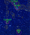 |
Fig. 1. Four HI clumps in the Leo ring where deep searches for the CO J = 1–0 and J = 2–1 lines have been carried out with the IRAM-30 m telescope (green circles). The circle size is the FWHM of the 115 GHz beam (22 arcsec). More than one location has been observed in Clump1 and Clump2E where Hα emission has been recently detected (see Figs. 2 and 3). The yellow contours indicate the column density of the HI gas in the giant Leo ring as observed with the VLA (45 arcsec beam) by Schneider et al. (1986). The magenta dashed circles indicate the location of the wobble OFF positions. The background image is the GALEX far-UV image. |
For every pointed observation our aim was to reach a spectral noise σ ≤ 5 mK in the averaged spectra for one of the two CO lines when smoothed at a spectral resolution δV = 2 km s−1. We list in Table 1 the coordinates of the 11 regions where we achieve this goal; deep pointed observations were carried out for every position during at least two distinct runs. The final rms in the CO J = 1–0 spectra ranges between 1.1 mK in C1a and 5 mK in C1an, which means that the spectral sensitivity is between 27 and 6 times better than previous observations carried out by Schneider et al. (1989). In addition, the large FCRAO beam is more strongly affected by beam dilution having a four times larger beam area.
Coordinates of selected regions of the Leo ring and the rms σ of CO spectra sampled at 2 km s−1 channel width.
In Figs. 2 and 3 we show zoomed-in images of the regions of Clump 1 and Clump 2E where more than one position has been observed. We indicate the observed positions with a continuous and dashed red circle, where the size is the FWHM of the IRAM beam at 115 and 230 GHz, respectively. In the background we display the location of the Hα counterparts observed with MUSE at VLT and the far-UV (FUV) counterparts detected by the GALEX satellite. In Table 1 we also show the rms of stacked spectra, obtained by averaging spectra at different but spatially close locations. These are C1ab, resulting from averaging C1a, C1b, C1an, C1ase; C1cl, resulting from averaging Cl1 and C1c; and C2E, resulting from averaging C2Ea, C2EB, and C2Ef. Clump 2 and BST have just one pointed observation; for Clump 2 the observed position is that of the nominal HI peak (Schneider et al. 1986), while for BST we selected BSTD, the location of a faint FUV region with no optical counterpart (to avoid contamination by background galaxies).
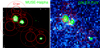 |
Fig. 2. Contours of the Hα emission of the three ionized regions in Clump1 (C1a, C1b, and C1c) overlaid (in green) on the MUSE-Hα image (left panel) and on the GALEX-FUV continuum image (right panel). The contour levels are 1.3, 2.5, 5, 10, 15×10−20 erg s−1 cm−2 per pixel (0.2″). The red continuous lines indicate the size of the 230 GHz beam FWHM at the locations observed in Clump1 with the IRAM-30 m telescope. The dashed red lines show the corresponding FWHM of the 115 GHz beam. The observed position labels are placed just outside the continuous red line circles. |
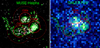 |
Fig. 3. Contours of the Hα emission of the two ionized regions in Clump2E, and of the partial ring overlaid (in green) on the MUSE-Hα image (left panel) and on the GALEX-FUV continuum image (right panel). The contour levels are 1.3, 2.5, 5, 10, 25×10−20 erg s−1 cm−2 per pixel (0.2″). The red continuous lines indicate the size of the 230 GHz FWHM IRAM-30m telescope beam at the observed locations in Clump2E. The dashed red lines show the corresponding FWHM of the 115 GHz beam. The observed position labels are placed just outside the continuous red line circles. |
The value of sigma was computed in the heliocentric velocity range 800–1200 km s−1. A robust detection would show peak intensity above 5σ in one of the lines with the second line at least marginally detected with peak or integrated line brightness above 3σ. We do not have any robust detections, only a few marginal detections. Given the velocities of the Hα lines, we consider as marginal detections the CO lines that lie in the velocity range 900–1100 km s−1 and that fulfill one of the following criteria: (1) the peak intensity or the integrated line brightness is above 3σ and lies within ±20 km s−1 of the mean Hα velocity of the nearest HII regions or HI peaks; (2) the peak intensity or the integrated line brightness is above 3σ for both the CO J = 1–0 and J = 2–1 lines; (3) the peak intensity or the integrated line brightness is above 4σ for only one of the lines.
In Table 2 we show all the lines that satisfy one of the above criteria and their estimated parameters. In that Table we list (from left to right): the name of the region and the CO line observed; the spectral resolution and the rms of the spectrum at that resolution in the 100 km s−1 interval around the line; the sum of the line emission in the spectral window of the signal in main beam units; the integrated emission of a Gaussian line fitted to the signal; the main beam peak temperature and the FWHM of the Gaussian fitted to the line; its peak velocity in the heliocentric reference system. In the last column we show for reference the heliocentric peak velocity of the Hα line detected at the same location, except for Cl2 where the Hα line is undetected and we show the HI line peak velocity. We have two marginal detections at the location of C1a and C1b, the two HII regions in Clump 1, whose spectra are shown in Figs. 4 and 5. In C1a, the line for the J = 1–0 transition looks more promising than the higher level transition. The remarkably low rms level of the C1a spectra required 72 h of telescope time. No J = 2–1 counterpart is detected for the 12CO J = 1–0 line marginally detected in C1b and shown in Fig. 5. For Cl2 J = 1–0 line we find similar parameters and integrated signal-to-noise ratio by choosing a spectral resolution δv = 0.5 or δv = 1.0 km s−1. In Table 2 and in Fig. 5 we show the results for the lowest spectral resolution for which we have the highest signal-to-noise ratio for the line peak. However, the peak velocity for Cl2 is higher by about 100 km s−1 than the velocity of the HI peak. This, and the high value of σ2 − 1, which does not allow us to detect a possible J = 2–1 line counterpart, casts some doubt on the effective presence of CO emission at the observed location. Within the 1′×1 arcmin2 MUSE field entered on Clump 2 no Hα line has been detected. Unfortunately, the FUV emission lies about 30 arcsec from the HI peak of Clump 2 and is at the edge of the MUSE field, outside the FWHM of IRAM beams. Thus, we do not know if stars are currently forming in Clump 2. We note that in other positions, such as C1a and BSTD, when the rms level in the averaged spectrum was much higher than the final one shown in Table 1, there were marginally detected lines that were not confirmed by longer integrations. Given the wide search range we consider the marginal detection in Cl2 to be due to sporadic noise.
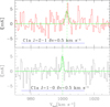 |
Fig. 4. Spectra of CO J = 1–0 (bottom) and J = 2–1 (top) at the position C1a for a spectral resolution of 0.5 km s−1. Gaussian fits to lines marginally detected with the highest integrated signal-to-noise emission are shown as a green line. The velocities of the Gaussian peaks are indicated by green vertical dashed lines. The horizontal blue lines at the bottom of each panel indicate the expected velocity range (as given by the C1a Hα line velocity ±20 km s−1). |
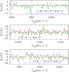 |
Fig. 5. Spectra of CO J = 1–0 at the positions of C1b (bottom) and Cl2 (middle) for 0.5 and 1 km s−1 channel width. The green lines show Gaussian fits to marginal detections with the highest integrated signal-to-noise emission. The velocities of the Gaussian peaks are indicated by green vertical dashed lines. The red dotted line shows the corresponding J = 2–1 spectra. The horizontal blue lines at the bottom of each panel indicate the expected velocity range (the Cl2 line is offset by more than 20 km s−1 from the velocity of the HI peak). The top panel shows the CO J = 1–0 stacked spectra of four adjacent positions in Clump1 (C1a, C1b, C1an, C1se). The Gaussian fit to the narrow negative dip (see text) is shown by the continuous green line. |
Parameters of the marginally detected 12CO lines.
Possible weak lines do not show up in the stacked spectra C1ab and this favors the hypothesis that the C1a and C1b lines are pseudo detections. The anomalous negative narrow line is not detected in individual spectra, although the analysis of C1a and C1b spectra at high resolution highlights that a very narrow line is present at the same velocity in C1a during two of the four observing periods. At the same time, a wider but fainter negative feature is present in the C1b spectra that might enhance the C1a feature when stacked spectra are produced. No features are present in the same channel at the higher frequency, and this excludes a possible problem with a particular correlation channel. Having a FWHM of only 0.5 km s−1 (line width confirmed at higher spectral resolution) it is also very unlikely that the line is due to diffuse CO emission at the location of the wobble throw. Since the specific location of the reference spectrum changes with source elevation, we do not expect possible gas at the throw locations to have a coherent velocity. The feature is likely the result of a local interference.
3. Candidate molecular clouds in Clump 1
In this section we discuss the marginally detected lines at the C1a and C1b locations in the proximity of Clump 1, as shown in Table 2 and Fig. 5. The spectral noise for these pointed observations is very low and a few very young massive stars are found at these locations. All cloud models mentioned in this section refer to the CO-bright parts of GMCs and for these, given the close-to-solar metallicity measured (12 + log O/H ≃ 8.6; Corbelli et al. 2021a), we assume a standard solar CO-to-H2 conversion factor XCO = 2 × 1020 cm−2 (K km s−1)−1. This converts the observed CO J = 1–0 intensity ICO into the beam diluted column density of molecular hydrogen, and it is equivalent to using the factor αCO = 4.3 M⊙ (K km s−1 pc2)−1 when inferring the molecular mass density. At the end of this section we also discuss the possibility of CO-dark gas.
The star-forming regions C1a and C1b are close to the peak of Clump 1, the largest HI overdensity in the main body of the ring at a mean heliocentric velocity of 987 km s−1 (Schneider et al. 1986). Their separation from the nominal position of the HI peak is 27 and 19 arcsec. These are very rough estimates given the 45 arcsec FWHM of the VLA beam used for mapping the 21 cm emission (Schneider et al. 1986). The nebula C1a is the second brightest HII region discovered by MUSE: the two CO line radial velocities are in full agreement with each other and with the velocities of the HI and HII gas (987 and 994 km s−1 respectively). For C1b we have an even better correspondence between the CO and the HI radial velocities (both at 987 km s−1). We infer the mass of molecular gas from the observed lines and its uncertainties, and then discuss the possible physical characteristics of a population of molecular clouds in the area.
We can write the molecular mass, which takes into account the contribution of heavy elements, as
 (1)
(1)
where SCO is the integrated line flux density in Jy km s−1, R21 is the intrinsic (2–1)/(1–0) line ratio (i.e., in brightness temperature), and DMpc is the distance to the source (in Mpc; Bolatto et al. 2013). The observed integrated line intensity ICO measures the beam diluted brightness temperature TbΔv = ICOΩs * b/Ωs, where the Ωs * b solid angle is the source convolved with the telescope beam, and it is equal to the telescope solid angle when the source is much smaller than the beam. We work under this assumption, and given the IRAM telescope parameters, we convert the intensity in K main beam temperature units into flux densities in Jy as
![Mathematical equation: $$ \begin{aligned} \frac{{{S_{{\rm{CO}}}}}}{{[{\rm{Jy}}{\mkern 1mu} {\rm{km}}{\mkern 1mu} {{\rm{s}}^{ - 1}}]}} = 5\;\frac{{{I_{{\rm{CO}}}}}}{{[{\rm{K}}{\mkern 1mu} {\rm{km}}{\mkern 1mu} {{\rm{s}}^{ - 1}}]}}. \end{aligned} $$](/articles/aa/full_html/2023/03/aa44941-22/aa44941-22-eq6.gif) (2)
(2)
Assuming that the emitting clouds in C1a and C1b are at the beam center, the observed CO line fluxes imply masses of 3.7 × 10⁴ M⊙ and 1.7 × 10⁵ M⊙ respectively (i.e., a total mass on the order of 2 × 10⁵ M⊙). This is lower than that estimated from the standard value of the gas consumption time discussed at the end of this section.
For sources that are offset with respect to the beam center, the molecular mass using Eq. (1) is underestimated. In M 33 the spatial correlation between infrared selected young stellar clusters and giant molecular clouds is strong, with a typical separation of 17 pc (Corbelli et al. 2017). This displacement, less than 1 arcsec at the distance of the Leo ring, would be negligible for the IRAM beams. Considering the nearest galaxies of the PHANGS sample (NGC 628, NGC 5068, NGC 5194, observed in the CO J = 2–1 line with good spatial resolution, similar to that of M 33), the separation between independent star-forming regions is on the order of 100 pc (Chevance et al. 2020). Similarly the nearest neighbor separation between massive GMCs and young stellar clusters in a larger PHANGS sample is found to be on the order of 100 pc (Turner et al. 2022). This suggests that the separation between HII regions and the associated native molecular clouds, or the molecular cloud formed by feedback, is expected to be on the order of 100 pc for Hα selected star-forming regions. This separation is much smaller than the beam HWHW at 115 GHz. Corrections to the observed flux become severe when the separation between the emitting object and the beam center is larger than the beam HWHM. Feedback effects might be stronger in the Leo ring than in galaxies, and we can use the HII region radius, on the order of 150 pc (3 arcsec), as a rough estimate for the expected cloud-HII region separation. Considering projection effects and pointing errors, on the order of 1.5 arcsec, the cloud–beam center offsets are expected to be less than 6 arcsec. This can reduce the flux recovered for the CO J = 2–1 line by up to about 50%, but the effects on the CO J = 1–0 line are much smaller.
3.1. Relating cloud physical parameters
To estimate the cloud radii in parsecs, Rpc, we use the virial theorem assuming a cloud density profile and a virial-to-CO luminous mass ratio. For ρ ∝ r−1 we have
 (3)
(3)
where the FWHM is in km s−1 (Bolatto et al. 2013). Assuming that Mvir/MCO = 1.0, as is often observed in galaxies (Bolatto et al. 2013), and using the FWHM of the marginal detections, we infer very large cloud radii (136 and 206 pc for C1a and C1b respectively). These radii, given the cloud mass, imply extremely low molecular gas volume densities, which are unphysical given the inefficient formation of molecules when gas densities are below 30 cm−3 (Hu et al. 2022). In addition, the marginally detected lines are narrow for their observed brightness, and not compatible with the standard size–linewidth relation which reads (Bolatto et al. 2013)
 (4)
(4)
with CSL = 0.37 pc (km s−1)−2 and which implies parsec-size clouds for the observed linewidths. The standard size–linewidth relation predicts cloud masses that scale with radius or FWHM as follows:
 (5)
(5)
In this case the cloud mass surface density is
 (6)
(6)
This is constant and on the order of 162 M⊙ pc−2 (Bolatto et al. 2013), much higher than the 0.6 M⊙ pc−2 we estimate at C1a. Any additional mass, such as CO-dark mass in a virialized cloud core or any mass corrections for cloud offsets with respect to the beam center, will increase the deviations from the size–linewidth relation observed in galaxies.
3.2. Standard cloud model
The CO lines shown in Table 2 are tentative detections with large uncertainties. In this subsection we assume that lines listed in Table 2 are not true detections, but false signals driven by sporadic noise. In this case, by considering clouds with physical parameters similar to those in galaxies, undetected because their emission is below the detection threshold, we can derive upper limits to their masses. The data on the J = 2–1 line are not used in this section because of uncertainties in the intrinsic line ratio (gas densities might not be sufficiently high that collisional equilibrium is reached for this higher level line), and because of possible cloud displacements with respect to the smaller 230 GHz beam. The J = 2–1 data is examined in the next section when we consider the beam diluted molecular gas surface brightness.
For the standard model we assume that the size–linewidth relation observed in galaxies and described by Eq. (4) applies. If a population of clouds with cloud masses lower than Mmax is in place we can compute Mmax from the rms of the observed spectra. We focus here on the C1a and C1b areas. We compute the maximum mass as a function of the J = 1–0 spectral rms σmK in mK at a spectral resolution δv in km s−1 as follows:
 (7)
(7)
Setting this maximum mass equal to Mvir we have that
 (8)
(8)
Substituting this expression for the FWHM into Eq. (7) for δv = 2 km s−1 we have Mmax as a function of the values of σmK quoted in Table 1, which reads
 (9)
(9)
The lowest value of Mmax is 9 × 10⁴ M⊙ for C1a, where we have the lowest noise; the highest value of Mmax is 5 × 10⁵ M⊙ at C1an. The upper limit Mmax in C1a is higher than the tentatively detected mass because of the wider line considered. If clouds are not at the beam center but within the beam FWHM, a slightly higher maximum mass should be considered.
In the left panel of Fig. 6 we show the FWHM and Mvir as a function of cloud radius Rpc for the standard model considered. The upper limits to C1a and C1b are shown as red crosses. For comparison, we also plot a scaled version of Eq. (4) obtained by replacing the coefficient CSL with a smaller constant value which fits the marginally detected CO J = 1–0 line in C1a. Although this model, referred to as the swollen model, is in agreement with the pseudo-lines in the spectra of C1a and C1b, we see that it predicts densities that are too low for the gas to be molecular. In the right panel of the same figure we show the average molecular hydrogen number density and the molecular mass surface density in the clouds (computed as the ratio of the cloud mass MCO to the cloud virial volume or area) for the same models as a function of the cloud viral mass.
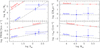 |
Fig. 6. Predicted relations between cloud parameters for the swollen and the standard cloud model. Left panels: cloud viral radius in relation to the line FWHM (bottom panel) and to the cloud viral mass (upper panel) according to the standard cloud model. The long dashed line is for the swollen model, which reproduces the tentative detections. Right panels: cloud viral mass in relation to the average volume density (bottom panel) and mass surface density (upper panel) for the standard and the swollen model. The tentative detections for C1a and C1b are shown as blue triangles for the swollen mode in each panel. For the standard model we only have upper limits which are shown by cross symbols with red arrows. |
3.3. CO-dark gas and the gas self-shielding conditions
It is clear from Fig. 6 that the marginally detected lines predict mean cloud densities that are three orders of magnitude lower than values for standard clouds observed in galaxies. This casts some doubt on the ability of gas to form molecules and to self-shield them from UV radiation from the nearby massive stars. If UV radiation from an HII region or from the interstellar field is incident on a neutral cloud, H2 molecules can reach high fractional abundance only after one magnitude of visual extinction, while CO is found deeper in denser clumps, where AV > 2 mag or NH > 4 × 1021 cm−2 (Hollenbach & Tielens 1999). Estimates of the visual extinction, made through the Balmer decrement observed in optical spectra, give AV ∼ 0.5 (Corbelli et al. 2021b). The presence of CO-dark envelopes can increase the cloud column density and attenuate the UV radiation field. Numerical simulations have shown that these envelopes are very common when gas volume densities are low, even for metal abundances close to solar (Hu et al. 2022). However, CO-dark envelopes lower the star formation efficiency (SFE) but do not help solve the problem of the low number gas densities in CO-bright clumps. The low gas densities suggest low fractional abundances of molecular hydrogen and long free-fall times.
Theoretically, the detailed formation-dissociation balance for H2 and CO molecules depends on the ratio n/G, where n is the gas volume density and G is the intensity of the UV radiation field. The radii of the C1a and C1b HII regions are about 200 and 100 pc, respectively. Given the stellar mass and age of their associated stellar clusters (Corbelli et al. 2021b), we estimate a UV interstellar radiation field at the edge of the HII regions that is between 10 and 5 times lower than in our local interstellar medium. As n/G decreases, the molecule’s fractional abundances decrease. If a few small dense clumps are floating in a large more massive diffuse cloud, mostly atomic, the whole cloud might show a low mean molecular fraction (if pressure supported or self-gravitating). However, the marginally detected lines can hardly refer to clumps floating in a diffuse clouds given the 10 km s−1 FWHM for HI lines usually observed in the ring (Schneider et al. 1986), although high resolution HI data are needed to verify that these large FWHMs also apply to hundred parsec scale regions.
The considerations expressed in this subsection suggest that the marginally detected lines should be considered with extreme caution and are likely due to sporadic noise. Future investigations through HI and CO observations at high spatial resolution, as well as specific theoretical models, are needed to test the turbulence level and other properties of dense gas fragments that form the sparse populations of stars in the Leo ring.
4. The star formation law at its lowest extreme
The relevance of CO detections in the Leo ring is not only related to understanding the physics and chemistry of cold gas overdensities forming stars in quiescent intergalactic clouds, but also to the fact that any detection might represent the lowest extreme ever observed for the molecular K–S law (Kennicutt & Evans 2012). It might confirm or refute the universality of such relation when the star formation rate surface density is lower than in outer disks or gas is not rotationally supported. We test the molecular K–S law considering upper limits for the CO lines and the standard cloud model for all IRAM-30 m pointed observations of star-forming regions in the Leo ring. We note that results are similar if future observations should confirm the marginally detected lines. We compare the gas consumption time and the star formation efficiency determined in disk galaxies to estimates for the Leo ring star-forming regions.
4.1. The molecular Kennicutt–Schmidt relation
We consider the six pointed observations listed in Table 1 that cover star-forming regions imaged by MUSE and have σ1 − 0, 2 − 1 ≤ 5: C1a, C1b, C1ase, C2Ea, C2Eb, C2ef. For these regions we performed circular aperture photometry in Hα to measure the SFR and its surface density, ΣSFR. We chose two apertures with the same angular size as the IRAM beam solid angle at 115 GHz and at 230 GHz (circular apertures with radii of 6.6 and 13.2 arcsec respectively). For the larger beam the emission in C1a and C1b is the same at both locations; it gives a SFR of 8 × 10⁻⁴ M⊙ yr−1 using the conversion factor in Table 3 of Corbelli et al. (2021b) for Mup = 35 M⊙, which reads
![Mathematical equation: $$ \begin{aligned} {{ \mathrm{SFR}_{\rm H\alpha }}\over [M_\odot \,\mathrm{yr}^{-1}]} = 1.9 \times 10^{-41}{L_{\rm H\alpha }\over [\mathrm{erg\,s}^{-1}]} .\end{aligned} $$](/articles/aa/full_html/2023/03/aa44941-22/aa44941-22-eq14.gif) (10)
(10)
The limiting mass for the upper end of the IMF was determined by Corbelli et al. (2021b) by comparing optical data with simulated stellar cluster models. Similar upper mass limits have been derived for the young population in outer disks (Bruzzese et al. 2020). We correct for an average visual extinction AV = 0.5. Uncertainties on the SFR are on the order of 0.5 dex, mostly driven by stochasticity due to incomplete sampling at the high mass end of the IMF (Corbelli et al. 2021b). The star formation rate density in C1a and C1b is 0.6 × 10⁻⁴ M⊙ yr−1 kpc−2 in the 115 GHz beam. We computed the star formation rate density for all the star-forming regions listed in Table 1.
To evaluate the molecular mass in the same aperture, we used the data in Table 1. We assume an intrinsic line ratio R = 2–1/1–0 = 0.5 and also use the data of the J = 2–1 spectra. We computed the molecular mass surface density in the beam assuming that the source is much smaller than the beam as
 (11)
(11)
where ΣCO is the cloud column density and MCO is the cloud mass inferred from CO integrated emission line. The beam solid angle Ωb is 1.2 × 10⁶ and 3 × 10⁵ pc2 for the IRAM beam at 115 and 230 GHz, respectively, at the distance of the Leo ring. The expression in Eq. (11) is equivalent to multiplying directly the integrated main beam temperature by the CO-to-H2 conversion factor (i.e., it measures the mean mass surface density also in the case of a population of low mass clouds in the beam).
We use the standard cloud model to derive the limiting mass surface densities for all six regions, as in Eq. (7), considering the C1a and C1b lines as spurious noise and the standard cloud model to infer FWHMlim. This is the FWHM of the most massive cloud compatible with the data which is computed following Eqs. (7) and (8):
 (12)
(12)
From these equations we find FWHMlim and the associated limiting mass
 (13)
(13)
The line FWHM in this case is generally smaller than 10 km s−1, varying between 5.3 and 8.1 km s−1 for the six star-forming regions considered in this paper. We computed the upper limits to the average molecular mass surface densities in the IRAM beams for these six regions; these values are plotted in the K–S diagram in Fig. 7. The solid straight line fits the data of the molecular mass surface densities of galaxies as given by Leroy et al. (2013). The dotted lines show the dispersion around the fitted line. At lower densities we show the range of Σmol for outer disks according to the data collected by Watson et al. (2016). The Leo ring data are at extremely low values of molecular gas surface densities and star formation rate densities, where the K–S relation has not been tested yet. A similar relation for the atomic gas surface densities is shown by Corbelli et al. (2021b) and implies extremely long depletion times (DTs) for the HI gas.
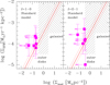 |
Fig. 7. K–S diagram relating star formation rates to molecular gas surface densities. The upper limits to the average molecular mass surface densities in the IRAM beams for six star-forming regions observed in the Leo ring are shown with magenta square symbols. The standard cloud model for the expected FWHM of the lines has been used. The continuum and dotted lines show the K–S relation and its dispersion, as fitted by Leroy et al. (2013) to the inner disk data of galaxies. The shaded areas indicate the molecular gas surface densities typical of the inner regions of galaxies and of outer disks (see Watson et al. 2016). |
Figure 7 indicates that most of the regions lie above the K–S relation. In particular the location of C1a (the leftmost star-forming region) and that of C2Ea (the region with the highest SFR density) in Fig. 7 seem incompatible with an extrapolation of the molecular K–S law towards low density regions. This inconsistency, evident both for the J = 1–0 line and for the J = 2–1 line, is then independent from the cloud model considered. The beam area for the J = 1–0 line is on the order of 1.2 kpc2, 50 times larger than the size of the HII regions, and on the same order as the scale sampled by Leroy et al. (2013). The surface density of molecular gas is lower than expected and implies a very short molecular gas depletion time, in contrast to the atomic gas depletion time.
4.2. Star formation efficiency and gas consumption times
The average DT and the SFE are usually defined and related to each other as
 (14)
(14)
where M* is the stellar mass of the young stellar cluster born in a molecular cloud of mass Mmol, and τGMC is the active lifetime of molecular clouds. Sometimes the star formation efficiency per free-fall time is used by substituting τGMC with the free-fall time at a given spatial resolution.
The average gas depletion time is observed to be relatively constant in nearby spiral and tidal dwarf galaxies and equal to 109.2 yr (Bigiel et al. 2011; Schruba et al. 2011; Lisenfeld et al. 2017). Given the SFR measured by Corbelli et al. (2021b), for each region considered in this paper, a DT similar to that observed in disk galaxies implies molecular masses in the range 0.4–4 × 10⁶ M⊙. Our most sensitive observations show that these masses are overestimated. For the case of C1a the depletion time is on the order of 3 × 10⁸ yr, a factor of 5 lower than in galaxies. Similar conclusions hold if molecular clouds are small but widespread, as in outer disks (Corbelli et al. 2017, 2019). In this case we expected an average molecular gas surface density of order 0.5 M⊙ pc−2 (Heyer & Dame 2015), higher than observed in the Leo ring, not compatible with the most sensitive data analyzed in this paper.
We can compute the SFE as the ratio of the stellar mass of young clusters to the mass of the nearest molecular cloud (i.e., assuming that the cluster progenitor cloud has a similar mass to other clouds in the cluster proximity). The estimated cluster masses at C1a and C1b are in the range 500–1000 M⊙ and we expect progenitor clouds to have masses in the range 5–10 × 104 M⊙ for a typical star formation efficiency of 1%. Therefore, clouds similar to those progenitors should have been detected by the deep integration performed in the C1a, even for the standard cloud model. Lower Mmol implies a higher SFE.
Cloud active lifetimes on the order of 10–20 Myr are measured by associating molecular clouds detected in deep survey of nearby galaxies with embedded (only infrared radiation detected) and exposed (with detectable Hα or optical continuum emission) young stellar clusters and by determining the age of the exposed clouds (Kawamura et al. 2009; Corbelli et al. 2017). A 10 Myr active lifetime and the measured DT give a SFE on the order of 3%, only slightly higher than determined by observations and theoretical models of bright spirals (Dobbs & Pringle 2013; Utomo et al. 2018). A somewhat shorter cloud lifetime is more in agreement with standard SFE values.
We can therefore conclude, using the data for the young and more active star-forming regions of the Leo ring, that molecular clouds form stars for a shorter period in the ring’s low density environment than in disk galaxies. The shorter star formation timescale indicates that clouds might be easier to dissolve as stellar feedback switches on and, more in general, that the gas-to-star conversion process in the Leo ring might depart from that studied extensively in disk galaxies. This might explain the nature of ultra diffuse dwarf galaxies. If molecular clouds dissolve quickly, or have a very high efficiency in forming stars, they will hardly be detected close to young stellar clusters. Our analysis shows that the decrease in the molecular gas depletion time observed from spiral to dwarf galaxies might not only be due to a decrease in the gas metallicity, but also to variations in the local conditions, such as a decrease in stellar mass and angular momentum, as previously claimed (Saintonge et al. 2011; Leroy et al. 2013; Hunt et al. 2015). The possibility of CO-dark gas in a low density but solar metallicity environment, such as the Leo ring, needs to be investigated in more detail, and might be linked to a change in the cloud’s physical conditions. The formation of stars from atomic gas should also be considered in case future more sensitive observations do not confirm the presence of molecular clouds (Krumholz 2012; Glover & Clark 2012). Sparse CO-bright dense clumps in extended self-gravitating atomic envelopes might be progenitors of the sparse population of young stars forming in Clumps 1.
5. Summary and conclusions
The close-to-solar metallicity recently determined for the giant HI ring in Leo has helped us solve the mystery of the ring origin, but at the same time the discovery of a sparse population of massive young stars has triggered new questions, for example why the gas in this collisional ring has not been forming stars since it was stripped from its progenitors, how stars form in an environment more quiescent than a galactic disk, if massive giant molecular clouds exist, and how efficiently they form stars. Moreover, the question of whether stars are born in clusters, associations, or in isolation in such an environment still needs to be investigated.
In this paper we presented the results of deep pointed observations of CO J = 1–0 and J = 2–1 lines in recently discovered star-forming regions of the Leo ring and close to its two most prominent HI peaks. These observations reached a spectral sensitivity that is between 27 and 6 times better than previous observations of the CO J = 1–0 line (Schneider et al. 1989). The new data sensitivity is sufficiently high to possibly detect the expected beam diluted molecular gas surface density, given the observed star formation rate density. The relation between the gas mass surface density and the star formation rate density has never been tested for such extremely low SFR densities as observed in the Leo ring.
For 11 pointed observations we reached a spectral noise between 1 and 5 mK main beam temperature, at least in one observed frequency when spectra are smoothed at 2 km s−1 resolution. The most sensitive observations were carried out for C1a, a region where stars are forming at a rate on the order of 10−4 M⊙ yr−1 kpc−2. The average mass surface density of molecular hydrogen in the 115 GHz beam expected from the extrapolation of the observed K–S relation in resolved star-forming galaxies should be higher than 0.1 M⊙ pc−2. The marginally detected line gives instead a lower mass surface density, only 0.03 M⊙ pc−2. If this marginal detection is spurious noise we derive a similar upper limit: 0.04 M⊙ pc−2. For the most active star-forming region found in the ring, C2Ea, the star formation rate density is 5 × 10⁻⁴ M⊙ yr−1 kpc−2 in the 230 GHz beam, but the surface density of molecular hydrogen is more than three times lower than expected.
The IRAM-30 m sensitive observations imply that the physical parameters of the star formation process in the Leo ring might deviate from those established in disk galaxies. We summarize below a few scenarios, that might explain deviations from the K–S law:
-
The molecular gas depletion timescale is short or, equivalently, gas condensations are very efficient in forming stars in the Leo ring. The gas in giant molecular clouds is more likely to rapidly dissolve or the low star formation rate and the lack of rotation might favor the formation of only low mass clouds with a high SFE.
-
The mass of CO-bright clumps might only be a fraction of the cloud mass that collapses and fragments to make stars. This implies the presence of CO-dark molecular gas or that collapsing gas is not fully molecular.
-
The mean separation between HII regions and the nearest giant molecular clouds might be larger than 500 pc because of efficient stellar feedback; molecular clouds in this case escaped detection because of the limited spatial coverage of IRAM-30 m pointed observations.
-
The stellar IMF might deviate from the power law observed in galaxies by suppressing gas fragmentation, or gas collapse, at low masses. The decrease in the estimated star formation rate makes the gas depletion timescale longer. Although this runs counter to generally considered top-light IMFs for low mass stellar clusters, only deep fully resolved stellar color–magnitude diagrams could reduce this uncertainty through explicit star counting and mass estimation.
These conclusions hold regardless of whether the marginally detected lines in C1a and C1b are due to emission from swollen molecular clouds or to spurious noise. We note that the very narrow and uncertain line widths, the low signal-to-noise ratio, and the predicted low gas number densities cast doubt on the identification of the marginally detected lines as true line emission. For this reason we often considered upper limits to the CO emission consistent with the standard size–linewidth relation that holds for CO-bright virialized clouds in galaxies.
Our results indicate that the life cycle of molecular clouds in the Leo ring might be shorter than in disk galaxies or, equivalently, that the spatial offsets between a young stellar cluster and a new ongoing embedded star formation site are much larger than in disk galaxies. This might explain the nature of ultra diffuse dwarf galaxies. Future sensitive observations at higher spatial resolution with millimeter interferometers, such as ALMA, together with additional data from 21 cm and Hubble Space Telescope imaging, can help us determine if deviations of the Leo ring star formation law from the K–S relation are due to variations in the mass distributions of gravitationally bound molecular clouds or to variations in their physical characteristics. The abundant J = 3–2 CO detections in the outer disk of M 83 (Koda et al. 2022) suggest that other CO transitions may further clarify the physical state of the molecular ISM in extreme environments.
Acknowledgments
This work is based on observations carried out under project numbers 058-20, 164-20, 165-21 with the IRAM-30 m telescope. IRAM is supported by INSU/CNRS (France), MPG (Germany) and IGN (Spain). We thank the IRAM allocation time committee and IRAM-30 m operators during lockdown period for their kind assistance during remote observing.
References
- André, P., Arzoumanian, D., Könyves, V., Shimajiri, Y., & Palmeirim, P. 2019, A&A, 629, L4 [Google Scholar]
- Archer, H. N., Hunter, D. A., Elmegreen, B. G., et al. 2022, AJ, 163, 141 [NASA ADS] [CrossRef] [Google Scholar]
- Bacchini, C., Fraternali, F., Pezzulli, G., & Marasco, A. 2020, A&A, 644, A125 [NASA ADS] [CrossRef] [EDP Sciences] [Google Scholar]
- Bekki, K., Koribalski, B. S., Ryder, S. D., & Couch, W. J. 2005, MNRAS, 357, L21 [NASA ADS] [Google Scholar]
- Bigiel, F., Leroy, A., Walter, F., et al. 2010, AJ, 140, 1194 [NASA ADS] [CrossRef] [Google Scholar]
- Bigiel, F., Leroy, A. K., Walter, F., et al. 2011, ApJ, 730, L13 [NASA ADS] [CrossRef] [Google Scholar]
- Bolatto, A. D., Wolfire, M., & Leroy, A. K. 2013, ARA&A, 51, 207 [CrossRef] [Google Scholar]
- Braine, J., Lisenfeld, U., Due, P.-A., & Leon, S. 2000, Nature, 403, 867 [Google Scholar]
- Bruzzese, S. M., Thilker, D. A., Meurer, G. R., et al. 2020, MNRAS, 491, 2366 [NASA ADS] [CrossRef] [Google Scholar]
- Chevance, M., Kruijssen, J. M. D., Hygate, A. P. S., et al. 2020, MNRAS, 493, 2872 [NASA ADS] [CrossRef] [Google Scholar]
- Corbelli, E., Bianchi, S., Cortese, L., et al. 2012, A&A, 542, A32 [NASA ADS] [CrossRef] [EDP Sciences] [Google Scholar]
- Corbelli, E., Braine, J., Bandiera, R., et al. 2017, A&A, 601, A146 [NASA ADS] [CrossRef] [EDP Sciences] [Google Scholar]
- Corbelli, E., Braine, J., & Giovanardi, C. 2019, A&A, 622, A171 [NASA ADS] [CrossRef] [EDP Sciences] [Google Scholar]
- Corbelli, E., Cresci, G., Mannucci, F., Thilker, D., & Venturi, G. 2021a, ApJ, 908, L39 [Google Scholar]
- Corbelli, E., Mannucci, F., Thilker, D., Cresci, G., & Venturi, G. 2021b, A&A, 651, A77 [NASA ADS] [CrossRef] [EDP Sciences] [Google Scholar]
- da Silva, R. L., Fumagalli, M., & Krumholz, M. R. 2014, MNRAS, 444, 3275 [Google Scholar]
- de los Reyes, M. A. C., & Kennicutt, R. C., Jr. 2019, ApJ, 872, 16 [NASA ADS] [CrossRef] [Google Scholar]
- Dobbs, C. L., & Pringle, J. E. 2013, MNRAS, 432, 653 [NASA ADS] [CrossRef] [Google Scholar]
- Donahue, M., Aldering, G., & Stocke, J. T. 1995, ApJ, 450, L45 [NASA ADS] [CrossRef] [Google Scholar]
- Elmegreen, B. G. 2015, ApJ, 814, L30 [Google Scholar]
- Elmegreen, B. G., & Hunter, D. A. 2015, ApJ, 805, 145 [NASA ADS] [CrossRef] [Google Scholar]
- Glover, S. C. O., & Clark, P. C. 2012, MNRAS, 421, 9 [NASA ADS] [Google Scholar]
- Heyer, M., & Dame, T. M. 2015, ARA&A, 53, 583 [Google Scholar]
- Hollenbach, D. J., & Tielens, A. G. G. M. 1999, Rev. Mod. Phys., 71, 173 [Google Scholar]
- Hu, C.-Y., Schruba, A., Sternberg, A., & van Dishoeck, E. F. 2022, ApJ, 931, 28 [NASA ADS] [CrossRef] [Google Scholar]
- Hunt, L. K., García-Burillo, S., Casasola, V., et al. 2015, A&A, 583, A114 [NASA ADS] [CrossRef] [EDP Sciences] [Google Scholar]
- Israel, F. P. 2005, A&A, 438, 855 [NASA ADS] [CrossRef] [EDP Sciences] [Google Scholar]
- Kawamura, A., Mizuno, Y., Minamidani, T., et al. 2009, ApJS, 184, 1 [NASA ADS] [CrossRef] [Google Scholar]
- Kennicutt, R. C., & Evans, N. J. 2012, ARA&A, 50, 531 [NASA ADS] [CrossRef] [Google Scholar]
- Kibblewhite, E. J., Cawson, M. G. M., Disney, M. J., & Phillipps, S. 1985, MNRAS, 213, 111 [Google Scholar]
- Kim, M. J., Chung, A., Lee, J. C., et al. 2015, Publ. Korean Astron. Soc., 30, 517 [Google Scholar]
- Koda, J., Watson, L., Combes, F., et al. 2022, ApJ, 941, 3 [NASA ADS] [CrossRef] [Google Scholar]
- Krumholz, M. R. 2012, ApJ, 759, 9 [NASA ADS] [CrossRef] [Google Scholar]
- Krumholz, M. R. 2013, MNRAS, 436, 2747 [CrossRef] [Google Scholar]
- Krumholz, M. R., Dekel, A., & McKee, C. F. 2012, ApJ, 745, 69 [Google Scholar]
- Lamers, H. J. G. L. M., Panagia, N., Scuderi, S., et al. 2002, ApJ, 566, 818 [NASA ADS] [CrossRef] [Google Scholar]
- Leroy, A. K., Walter, F., Sandstrom, K., et al. 2013, AJ, 146, 19 [Google Scholar]
- Leroy, A. K., Schinnerer, E., Hughes, A., et al. 2021, ApJS, 257, 43 [NASA ADS] [CrossRef] [Google Scholar]
- Lisenfeld, U., Braine, J., Duc, P. A., et al. 2004, A&A, 426, 471 [NASA ADS] [CrossRef] [EDP Sciences] [Google Scholar]
- Lisenfeld, U., Alatalo, K., Zucker, C., et al. 2017, A&A, 607, A110 [NASA ADS] [CrossRef] [EDP Sciences] [Google Scholar]
- López-Sánchez, Á. R., Lagos, C. D. P., Young, T., & Jerjen, H. 2018, MNRAS, 480, 210 [CrossRef] [Google Scholar]
- Lutz, K. A., Saintonge, A., Catinella, B., et al. 2021, A&A, 649, A39 [NASA ADS] [CrossRef] [EDP Sciences] [Google Scholar]
- Michel-Dansac, L., Duc, P.-A., Bournaud, F., et al. 2010, ApJ, 717, L143 [Google Scholar]
- Mihos, J. C., Carr, C. T., Watkins, A. E., Oosterloo, T., & Harding, P. 2018, ApJ, 863, L7 [Google Scholar]
- Müller, O., Jerjen, H., & Binggeli, B. 2018, A&A, 615, A105 [Google Scholar]
- Pasha, I., Lokhorst, D., van Dokkum, P. G., et al. 2021, ApJ, 923, L21 [NASA ADS] [CrossRef] [Google Scholar]
- Pierce, M. J., & Tully, R. B. 1985, AJ, 90, 450 [Google Scholar]
- Querejeta, M., Lelli, F., Schinnerer, E., et al. 2021, A&A, 645, A97 [NASA ADS] [CrossRef] [EDP Sciences] [Google Scholar]
- Reynolds, R. J., Magee, K., Roesler, F. L., Scherb, F., & Harlander, J. 1986, ApJ, 309, L9 [NASA ADS] [CrossRef] [Google Scholar]
- Rood, H. J., & Williams, B. A. 1985, ApJ, 288, 535 [Google Scholar]
- Saintonge, A., Kauffmann, G., Wang, J., et al. 2011, MNRAS, 415, 61 [NASA ADS] [CrossRef] [Google Scholar]
- Schneider, S. 1985, ApJ, 288, L33 [Google Scholar]
- Schneider, S. E., Helou, G., Salpeter, E. E., & Terzian, Y. 1983, ApJ, 273, L1 [Google Scholar]
- Schneider, S. E., Salpeter, E. E., & Terzian, Y. 1986, AJ, 91, 13 [Google Scholar]
- Schneider, S. E., Skrutskie, M. F., Hacking, P. B., et al. 1989, AJ, 97, 666 [Google Scholar]
- Schruba, A., Leroy, A. K., Walter, F., et al. 2011, AJ, 142, 37 [NASA ADS] [CrossRef] [Google Scholar]
- Sil’chenko, O. K., Moiseev, A. V., Afanasiev, V. L., Chavushyan, V. H., & Valdes, J. R. 2003, ApJ, 591, 185 [Google Scholar]
- Stierwalt, S., Haynes, M. P., Giovanelli, R., et al. 2009, AJ, 138, 338 [Google Scholar]
- Tacconi, L. J., & Young, J. S. 1987, ApJ, 322, 681 [NASA ADS] [CrossRef] [Google Scholar]
- Tacconi, L. J., Genzel, R., & Sternberg, A. 2020, ARA&A, 58, 157 [NASA ADS] [CrossRef] [Google Scholar]
- Thilker, D. A., Bianchi, L., Meurer, G., et al. 2007, ApJS, 173, 538 [Google Scholar]
- Thilker, D. A., Donovan, J., Schiminovich, D., et al. 2009, Nature, 457, 990 [Google Scholar]
- Turner, J. A., Dale, D. A., Lilly, J., et al. 2022, MNRAS, 516, 4612 [NASA ADS] [CrossRef] [Google Scholar]
- Utomo, D., Sun, J., Leroy, A. K., et al. 2018, ApJ, 861, L18 [NASA ADS] [CrossRef] [Google Scholar]
- Watkins, A. E., Mihos, J. C., Harding, P., & Feldmeier, J. J. 2014, ApJ, 791, 38 [Google Scholar]
- Watson, L. C., Martini, P., Lisenfeld, U., Böker, T., & Schinnerer, E. 2016, MNRAS, 455, 1807 [CrossRef] [Google Scholar]
All Tables
Coordinates of selected regions of the Leo ring and the rms σ of CO spectra sampled at 2 km s−1 channel width.
All Figures
|
Fig. 1. Four HI clumps in the Leo ring where deep searches for the CO J = 1–0 and J = 2–1 lines have been carried out with the IRAM-30 m telescope (green circles). The circle size is the FWHM of the 115 GHz beam (22 arcsec). More than one location has been observed in Clump1 and Clump2E where Hα emission has been recently detected (see Figs. 2 and 3). The yellow contours indicate the column density of the HI gas in the giant Leo ring as observed with the VLA (45 arcsec beam) by Schneider et al. (1986). The magenta dashed circles indicate the location of the wobble OFF positions. The background image is the GALEX far-UV image. |
| In the text | |
|
Fig. 2. Contours of the Hα emission of the three ionized regions in Clump1 (C1a, C1b, and C1c) overlaid (in green) on the MUSE-Hα image (left panel) and on the GALEX-FUV continuum image (right panel). The contour levels are 1.3, 2.5, 5, 10, 15×10−20 erg s−1 cm−2 per pixel (0.2″). The red continuous lines indicate the size of the 230 GHz beam FWHM at the locations observed in Clump1 with the IRAM-30 m telescope. The dashed red lines show the corresponding FWHM of the 115 GHz beam. The observed position labels are placed just outside the continuous red line circles. |
| In the text | |
|
Fig. 3. Contours of the Hα emission of the two ionized regions in Clump2E, and of the partial ring overlaid (in green) on the MUSE-Hα image (left panel) and on the GALEX-FUV continuum image (right panel). The contour levels are 1.3, 2.5, 5, 10, 25×10−20 erg s−1 cm−2 per pixel (0.2″). The red continuous lines indicate the size of the 230 GHz FWHM IRAM-30m telescope beam at the observed locations in Clump2E. The dashed red lines show the corresponding FWHM of the 115 GHz beam. The observed position labels are placed just outside the continuous red line circles. |
| In the text | |
|
Fig. 4. Spectra of CO J = 1–0 (bottom) and J = 2–1 (top) at the position C1a for a spectral resolution of 0.5 km s−1. Gaussian fits to lines marginally detected with the highest integrated signal-to-noise emission are shown as a green line. The velocities of the Gaussian peaks are indicated by green vertical dashed lines. The horizontal blue lines at the bottom of each panel indicate the expected velocity range (as given by the C1a Hα line velocity ±20 km s−1). |
| In the text | |
|
Fig. 5. Spectra of CO J = 1–0 at the positions of C1b (bottom) and Cl2 (middle) for 0.5 and 1 km s−1 channel width. The green lines show Gaussian fits to marginal detections with the highest integrated signal-to-noise emission. The velocities of the Gaussian peaks are indicated by green vertical dashed lines. The red dotted line shows the corresponding J = 2–1 spectra. The horizontal blue lines at the bottom of each panel indicate the expected velocity range (the Cl2 line is offset by more than 20 km s−1 from the velocity of the HI peak). The top panel shows the CO J = 1–0 stacked spectra of four adjacent positions in Clump1 (C1a, C1b, C1an, C1se). The Gaussian fit to the narrow negative dip (see text) is shown by the continuous green line. |
| In the text | |
|
Fig. 6. Predicted relations between cloud parameters for the swollen and the standard cloud model. Left panels: cloud viral radius in relation to the line FWHM (bottom panel) and to the cloud viral mass (upper panel) according to the standard cloud model. The long dashed line is for the swollen model, which reproduces the tentative detections. Right panels: cloud viral mass in relation to the average volume density (bottom panel) and mass surface density (upper panel) for the standard and the swollen model. The tentative detections for C1a and C1b are shown as blue triangles for the swollen mode in each panel. For the standard model we only have upper limits which are shown by cross symbols with red arrows. |
| In the text | |
|
Fig. 7. K–S diagram relating star formation rates to molecular gas surface densities. The upper limits to the average molecular mass surface densities in the IRAM beams for six star-forming regions observed in the Leo ring are shown with magenta square symbols. The standard cloud model for the expected FWHM of the lines has been used. The continuum and dotted lines show the K–S relation and its dispersion, as fitted by Leroy et al. (2013) to the inner disk data of galaxies. The shaded areas indicate the molecular gas surface densities typical of the inner regions of galaxies and of outer disks (see Watson et al. 2016). |
| In the text | |
Current usage metrics show cumulative count of Article Views (full-text article views including HTML views, PDF and ePub downloads, according to the available data) and Abstracts Views on Vision4Press platform.
Data correspond to usage on the plateform after 2015. The current usage metrics is available 48-96 hours after online publication and is updated daily on week days.
Initial download of the metrics may take a while.