| Issue |
A&A
Volume 670, February 2023
|
|
|---|---|---|
| Article Number | A25 | |
| Number of page(s) | 10 | |
| Section | Stellar atmospheres | |
| DOI | https://doi.org/10.1051/0004-6361/202245503 | |
| Published online | 01 February 2023 | |
Non-local thermodynamic equilibrium analysis of the methylidyne radical molecular lines in metal-poor stellar atmospheres
1
Max-Planck-Institute for Astronomy,
Königstuhl 17,
69117
Heidelberg, Germany
e-mail: This email address is being protected from spambots. You need JavaScript enabled to view it.
2
Heidelberg University,
Grabengasse 1,
69120
Heidelberg, Germany
3
Laboratoire Univers et Particules de Montpellier, Univ Montpellier, CNRS,
Montpellier, France
4
Department of Physics and Astronomy and JINA Center for the Evolution of the Elements, University of Notre Dame,
Notre Dame, IN
46556, USA
Received:
18
November
2022
Accepted:
12
December
2022
Abstract
Aims. An analysis of the methylidyne (CH) radical in non-local thermodynamic equilibrium (NLTE) is performed for the physical conditions of cool stellar atmospheres typical of red giants (log ɡ = 2.0, Teff = 4500 K) and the Sun. The aim of the present work is to explore whether the G band of the CH molecule, which is commonly used in abundance diagnostics of carbon-enhanced metal-poor stars, is sensitive to NLTE effects.
Methods. LTE and NLTE theoretical spectra were computed with the MULTI code. We used one-dimensional (1D) LTE hydrostatic MARCS model atmospheres with parameters representing eleven red giant stars with metallicities ranging from [Fe/H] = −4.0 to [Fe/H] = 0.0 and carbon-to-iron ratios of [C/Fe] = 0.0, +0.7, +1.5, and +3.0. The CH molecule model was represented by 1981 energy levels, 18 377 radiative bound-bound transitions, and 932 photo-dissociation reactions. The rates due to transitions caused by collisions with free electrons and hydrogen atoms were computed using classical recipes.
Results. Our calculations suggest that NLTE effects in the statistical equilibrium of the CH molecule are significant and cannot be neglected for precision spectroscopic analysis of C abundances. The NLTE effects are mostly driven by radiative over-dissociation, owing to the very low dissociation threshold of the molecule and significant resonances in the photo-dissociation cross-sections. The NLTE effects in the G band increase with decreasing metallicity. When comparing the C abundances determined from the CH G band in LTE and in NLTE, we show that the C abundances are always under-estimated if LTE is assumed. The NLTE corrections to C abundance inferred from the CH feature range from +0.04 dex for the Sun to +0.21 dex for a red giant with metallicity [Fe/H] = −4.0.
Conclusions. Departures from the LTE assumption in the CH molecule are non-negligible, and NLTE effects have to be taken into account in the diagnostic spectroscopy based on the CH lines. We show here that the NLTE effects in the optical CH lines are non-negligible for the Sun and red giant stars, but further calculations are warranted to investigate the effects in other regimes of stellar parameters.
Key words: molecular data / molecular processes / radiative transfer / stars: carbon / stars: abundances / stars: late-type
© The Authors 2023
 Open Access article, published by EDP Sciences, under the terms of the Creative Commons Attribution License (https://creativecommons.org/licenses/by/4.0), which permits unrestricted use, distribution, and reproduction in any medium, provided the original work is properly cited.
This article is published in open access under the Subscribe-to-Open model.
Open access funding provided by Max Planck Society.
1 Introduction
In the last decades, there has been increasing interest in metal-poor stars in the Milky Way (MW) and its dwarf satellite galaxies (see Beers & Christlieb 2005 for a historical summary of the field at the time, and Frebel 2018 for a more recent review). Being the oldest stars that can be directly observed at present, they carry invaluable information about the early Galaxy, including initial conditions for star and galaxy formation (e.g. Klessen et al. 2012; Frebel & Norris 2015; Yoon et al. 2018), large galaxy assembly (e.g. Carollo et al. 2007, 2010; Beers et al. 2012), and the early history of nucleosynthesis (e.g. Hansen et al. 2011; Gil-Pons et al. 2021; Qian 2022).
As more and more metal-poor stars are observed, it has become clear that the frequency of stars that exhibit strong carbon enhancement (resulting in [C/Fe] = +0.7 or even higher) dramatically increases with decreasing metallicity. Beers & Christlieb (2005) classified such stars as carbon-enhanced metal-poor (CEMP) stars (using the criteria at the time of [Fe/H] < −1.0 and [C/Fe] > +1.0. The nature of the CEMP stars is reflected in their absolute carbon abundance (A(C); Spite et al. 2013; Yoon et al. 2016), as well as in their heavy-element content (e.g. Beers & Christlieb 2005; Frebel 2018; Hansen et al. 2019).
The nature and chemical composition of the CEMP stars is not yet well-defined, and has been targeted in numerous observational studies (e.g. Aoki et al. 2008, 2022; Yong et al. 2013; Ito et al. 2013; Lee et al. 2013; Masseron et al. 2014; Yoon et al. 2016; Rasmussen et al. 2020; Zepeda et al. 2022b). One subclass of CEMP stars exhibits very high levels of C combined with a strong enrichment in slow neutron-capture (s-) process elements and can be explained by mass transfer in a binary system from an asymptotic giant branch (AGB) star onto a smaller less evolved binary companion that we now observe as a CEMP-s star (e.g. Aoki et al. 2007; Placco et al. 2013; Starkenburg et al. 2014; Abate et al. 2015; Hansen et al. 2016b, Hansen et al. 2019; Caffau et al. 2019; Goswami et al. 2021). Another sub-class, the CEMP-no stars, shows absolute C abundances that are 1–3 dex lower than the CEMP-s stars, with no enhancements in neutron-capture elements. Although their origin is still debated, they are believed to be bona fide second-generation stars (e.g. Ryan et al. 2005; Hansen et al. 2016c; Zepeda et al. 2022a), where possible formation sites are polluted by massive, fast-rotating, ultra-metal-poor (UMP; [Fe/H] < −4.0) and hyper-metal-poor (HMP; [Fe/H] < −5.0) stars, also known as spinstars (Meynet et al. 2006; Choplin et al. 2017; Choplin & Hirschi 2020; Liu et al. 2021) or faint core-collapse supernovae that undergo mixing and fallback (e.g. Nomoto et al. 2013), leaving behind large amounts of lighter elements such as C but lower amounts of the heavy elements. This evidence makes CEMP-no stars candidates for the first low-mass stars to form in the early Universe (Hansen et al. 2016c,a).
Owing to the low metallicities of CEMP stars, the main diagnostic of the C abundance is the G band, which is the most prominent feature of the methylidyne (CH) radical in their optical spectra (Masseron et al. 2014). The G band is found around 4300 Å and it is also used as a diagnostic for the Morgan-Keenan (MK) classification scheme (Morgan et al. 1943). It consists of numerous molecular lines that arise from electronic transitions between the electronic ground state Χ2Π and the first excited electronic state A2Δ of the CH radical.
Past analyses of the CH G-band were carried out under the assumption of local thermodynamic equilibrium (LTE; e.g. Placco et al. 2016; François et al. 2018; Norris & Yong 2019), although it was shown early on that CH lines were formed out of LTE in the solar atmosphere (Eugène-Praderie & Pecker 1960). The LTE assumption greatly simplifies the complexity of the computations. However, it also fails to realistically describe the interaction between radiation and matter in stellar atmospheres (Bergemann & Nordlander 2014). This is instead achieved by non-LTE (NLTE) modelling, where the radiation field and the distribution of matter over different energy states are not simply given by their equilibrium values, as in LTE, but are explicitly determined by solving the coupled radiative transfer and statistical equilibrium equations.
This work presents the analysis of the NLTE statistical equilibrium for the CH radical. Our aim is to determine whether departures from LTE are significant, in particular for the conditions pertaining to cool, metal-poor stellar atmospheres.
The paper is organised as follows. The stellar atmospheres and the molecule model are presented in Sect. 2. The modelling of theoretical spectra of the CH molecule is presented in Sect. 3, along with the NLTE abundance corrections for representative model atmospheres for cool red giants of various metallicities and carbon enhancements. The results are discussed in the context of other works in Sect. 4 and are summarised in Sect. 5.
2 Methods
Due to the scarcity of literature on the NLTE modelling of molecules, we briefly recap the nomenclature. Electronic levels of molecular species are described by the orbital angular momentum Λ (Σ, Π, and Δ for 0, 1, 2 states, accordingly), vibrational quantum number v, rotational quantum number J, the total electron angular momentum Ω (sum of Λ and Σ, the electronic spin), and symmetry describing geometric operations (e/f). Following the standard notation in chemistry, we furthermore denote the ground state with a′ and an excited state with a″.
2.1 Model of the CH radical
The molecule CH is a heteronuclear diatomic molecule with an internuclear distance of 0.16 nm (Demtroeder 2003) and the binding energy of the ground state 2Π of 3.45 eV (Herzberg & Johns 1969). In our representation, the CH model contains 1981 energy levels, 18 377 radiative bound-bound transitions, and 932 photo-dissociation transitions. The data for energy states and bound-bound radiative transitions were taken from Masseron et al. (2014). The latter model does not include the a4Σ− state, as there are no bound-bound radiative transitions from this to other states of the molecule; therefore, this state was not included in our model either. The photo-dissociation cross-sections for the available states were adopted from Kurucz et al. (1987). In our model, we retained all energy states with distinct molecular quantum numbers. Whereas the original datasets comprise 52201 radiative transitions, to simplify the calculations we retained only transitions in the wavelength range from 1000 to 20 000 Å, as this covers the significant range of the spectral energy distribution of cool stars, and astrophysical line strengths larger than −5 (Fig. 1, top panel) computed using the following expression:
 (1)
(1)
where the energy of the lower level Elow is given in eV, wavelength λ in Å, and gf is the product of the oscillator strength f and the statistical weight of the lower level g, and T the temperature in Kelvin, here set to T = 4000 K. We also excluded the extremely weak transitions with f-values less than 10−7. Most of them connect energy states with small energy separations, and this may lead to numerical problems with population inversions in the statistical equilibrium calculations. In Fig. 1 (bottom panel), we also show the distribution of gf-values of the X– A transitions in the wavelength range around ~4300 Å, which is easily accessible by astronomical facilities. The P, Q, and R branches are indicated. The strongest feature in this range, corresponding to J′ − J″ = 0 (vibrational transition accompanied by a rotational transition) is the astrophysically famous 'G band'.
The energy levels included in the NLTE model are displayed in Figs. 2, 3, and 4 in the plane of J (rotational number) against level energy (in eV). Figure 2 shows the G-band lines arising in the transitions in the limited wavelength range from 4297 to 4340 Å, Fig. 3 shows the complete set of radiative bound–bound transitions included in the model, and Fig. 4 shows the photodissociation reactions. In our model, the photo-dissociation transitions take place between the ground state levels X2Π with energies of E = 0−3.17 eV, the rotational quantum numbers J = 0.5−45.5, and the vibrational quantum numbers υ = 0−5 and the dissociated state C + H. As evident from the plots, the electronic ground state, X2Π, is clearly separated from the other excited electronic states A2Δ, B2Σ−, and C2Σ+, which have an intertwined structure in this particular representation, where the energy of the levels is plotted against the rotational number J. These diagrams reveal the complexity of the energetic structure of molecules, with each electronic energy level consisting of finer vibrational energy levels and even finer rotational energy levels.
All bound energy levels were also connected through collisional transitions, where collisions with free electrons, as well as with hydrogen atoms, were considered. The collisional recipes assumed in our study are approximate (see e.g. Barklem 2016); however, for the lack of more accurate datasets, they provide a suitable starting point for exploring the effects of NLTE in the molecule. The rates of transitions caused by collisions with free electrons e− were computed using van Regemorter's formula for allowed transitions (van Regemorter 1962) and Allen's formula (Allen 1973) for forbidden transitions (log gf ≤ −10). The rate processes in bound-bound as well as bound-free transitions, caused by collisions with H atoms, were computed using Drawin's formula in the formulation of Steenbock & Holweger (1984). Limited theoretical studies of inelastic collisions of CH rotational fine-structure levels with molecular hydrogen exist (Dagdigian 2017); however, the temperatures considered (up to 300 K) are tailored to the conditions of the interstellar medium and are too low for the purposes of our study. Extrapolation of these datasets to stellar conditions is not advised (P. Dagdigian, priv. comm.). The results of NLTE calculations in CH might be sensitive to collisions. However, a more detailed study of this aspect would require direct quantum-mechanical estimates of rate coefficients at least for a subset of relevant transitions (especially, for the C + H reactions), and we defer such an analysis for future work, once such estimates become available for the conditions of atmospheres of FGK-type stars.
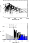 |
Fig. 1 Properties of the transitions in the CH molecule model. Top panel: distribution of line strengths in the entire CH system. Only transitions with strengths greater than S = –5 were included in the NLTE model molecule. Bottom panel: X–A spectrum of the CH molecule around the wavelength of ~4300 Å. The P, Q, and R branches are indicated. The strongest feature in this range, corresponding to J′ − J″ = 0 (vibrational transition accompanied by a rotational transition) is the astrophysically famous 'G band'. |
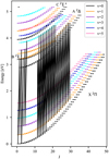 |
Fig. 2 Energy levels included in CH molecule model with specified rotational quantum number J and vibrational quantum number υ. The black lines indicate the bound-bound transitions between the electronic states A2Δ and X2Π that give rise to the molecular G-band lines in the wavelength 4297–4303 Å range. |
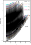 |
Fig. 3 Energy levels included in the CH molecule model with specified rotational quantum number J and vibrational quantum number υ. The black lines indicate all radiative bound-bound transitions included in the model. |
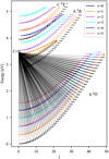 |
Fig. 4 Black lines indicate the transitions for the photo-dissociation reactions with the dissociation energy of 3.45 eV. |
2.2 Statistical equilibrium calculations
The calculations of NLTE statistical equilibrium and G-band spectra were done with the help of the MULTI code (Scharmer & Carlsson 1985; Carlsson 1986). This code was developed in order to solve NLTE radiative transfer problems in semi-infinite, one-dimensional (1D) atmospheres with a prescribed macroscopic velocity field, where the model atom can have many atomic levels and several ionisation stages. The code uses an approximate lambda iteration (ALI) method for the statistical equilibrium calculations, and the local version of the lambda operator was used in this work. All calculations were carried out taking line blanketing into account. Detailed opacities were computed as described in Bergemann et al. (2019) using the MARCS model atmospheres and Turbospectrum code (Plez 2012; Gerber et al. 2022) for a range of metal mixtures representative of the model atmospheres studied in this work. The line lists used for the opacity calculations include all chemical elements up to U in the first three ionisation stages (for more details, see Bergemann et al. 2013, Bergemann et al. 2015).
For the CH radical, transitions from the bound levels to the continuum level correspond to photo-dissociation processes, which represent the breaking of the CH molecule into its constituent atoms, C and H, as described by the following reaction:
 (2)
(2)
The necessary energy for this reaction to take place from the ground state is given by the threshold dissociation energy of 3.45 eV, which corresponds to the energy of ~1.6 eV below the last bound energy state of the molecule. The cross-sections for one of the energy states of CH is shown in Fig. 5. To compute the photo-dissociation rate coefficient, Rij, we followed the standard description of bound-free processes (e.g. Hubeny & Mihalas 2014):
 (3)
(3)
with ni being the number density of the CH level (i) that dissociates, j the level in the CI atom to which it dissociates (all dissociations in our model molecule end with the neutral C atom in its ground state), σij(v) the photo-dissociation cross-section, Jv the mean intensity of radiation, v0 the threshold energy, and v the frequency. The reverse reaction, namely the photo-attachment, which describes the formation of the CH molecule from individual C and H atoms, was computed assuming micro-reversibility as follows:
 (4)
(4)
where the star * symbol denotes LTE populations. Photo-attachment reactions can be associated with stimulated and spontaneous processes; in this equation, the factor J represents the induced photo-attachment and the factor 2hv3/c2 describes spontaneous transitions. The ratio  represents the ratio between the number density of CH molecules in the energy state i relative to the number density of C I atoms in the ground state, and it is computed as
 (5)
(5)
where nx and Qx are the total number densities and partition functions of the species x, g0 is the multiplicity of the C I ground state, and gi and Ei are the multiplicity and energy of a given CH level, i. The LTE C I level populations were computed using the Saha and Boltzmann equations. The CH number densities were calculated using the equilibrium constants from Tsuji (1973).
Photoionisation of CH is not important for the statistical equilibrium of the molecule, because of the very high ionisation potential of CH ground state (10.6 eV). This situation is analogous to O I, for which photo-ionisation processes and the details of the corresponding cross-sections have a negligible effect on the statistical equilibrium of the ion (Bergemann et al. 2021; Bautista et al. 2022).
 |
Fig. 5 Cross-section distribution of photo-dissociation for energy level at 2.45 eV (19777.31 cm−1) with the following configuration: electronic state X2Π with quantum numbers υ = 0 and J = 40. |
 |
Fig. 6 LTE and NLTE spectra in region of CH G band, computed using the model atmosphere with a solar carbon abundance of A(C) = 8.43. |
2.3 Model atmospheres
In this work, we used the MARCS model atmospheres (Gustafsson et al. 2008). The models represent giant K-type stars (log g = 2.0, Teff = 4500 K) with metallicities in the range of −4.0 ≤ [Fe/H] ≤ 0.0 and a microturbulence of 2 km s−1. They are computed under the assumption of LTE and hydrostatic equilibrium, using a 1D geometry with a spherical symmetry. We note that in this paper we limited the analysis to K giants, because these types of stars are commonly used for spectral diagnostics of carbon abundances at very low metallicity. Other spectral types and luminosity classes will be investigated in our upcoming papers.
Because of the assumptions of 1D hydrostatic equilibrium, these model atmospheres do not describe time-dependent 3D phenomena such as convection and turbulence; hence, additional parameters have to be introduced. In the models, convection is described using the mixing-length theory presented by Henyey et al. (1965), parametrised by α = l/Hp = 1.5, where l is the mixing length and  is the pressure scale height. Another parameter is the microturbulent velocity,, ξt, which describes turbulent motions on scales smaller than the photon's mean free path in the atmosphere. This parameter is taken to be 2 km s−1.
3 Results
Molecular spectra are more complex than atomic spectra, due to their more complicated energy structure given by the different electronic, vibrational, and rotational energy levels, and the numerous molecular transitions that can take place between them. These transitions give rise to numerous absorption lines, which, by overlapping, create the absorption bands that are characteristic of molecular spectra.
We analysed the properties of G-band spectra calculated in LTE and NLTE for the Sun and for cool red giant stars with different metallicities. All transitions that give rise to molecular lines in this range are displayed in Fig. 2.
3.1 Sun
The G band in the spectrum of the model atmosphere with the parameters of the Sun (Teff = 5777 K, log = 4.44, [Fe/H] = 0.0) is displayed in Fig. 6. The wavelength range between 4297 and 4303 Å was chosen since it allows us to both visually distinguish the line profiles and interpret the effects of NLTE. As the G-band is formed from the transitions between the same electronic energy states, any chosen wavelength region would lead to the same results. Both LTE and NLTE profiles were computed using a C abundance of A(C) = 8.43 (Asplund et al. 2009). Even though the same atmosphere and molecule model were used for the computation, the figure shows that the NLTE profile of the G band is weaker than the LTE profile across the entire considered wavelength range. The difference between the NLTE and LTE line profiles is caused by the differences in the distribution of particles over excitation stages an the dissociation of CH. Therefore, it is useful to make use of the concept of the departure coefficient, bi, for a level, i (e.g. Bergemann & Nordlander 2014):
 (6)
(6)
where  is the population given by the equilibrium Saha–Boltzmann distribution, and
  is the actual population computed iteratively using the statistical equilibrium equations. If bi = 1, the population is given by the LTE value and the level is said to be thermalised, whereas bi ≠ 1 indicates departure from LTE. If bi > 1, the level is over-populated, and if bi < 1 the level is under-populated with respect to the population given by the LTE assumption.
To illustrate the difference between the LTE and NLTE computation, we inspected a representative G-band line at 4299.48 Å (Fig. 7). It arises from the transition between the electronic state A2Δ with energy Ej = 3.2 eV, the rotational quantum number Jj = 1.5, and the vibrational quantum number υj = 1 and the ground state X2Π with Ei = 0.3 eV, Ji = 0.5, and υi = 1, respectively. The departure coefficients for the upper level j and lower level i of the representative line are displayed in the top panel of Fig. 8. In the deeper layers of the atmosphere (log τ500 ≳ 0), both levels are thermalised: bi = bj = 1. However, in the upper photospheric layers (log τ500 ≲ 0), the populations start to experience departures from the LTE assumption. This corresponds to our expectations, as the LTE assumption is known to only hold in the deeper layers of the stellar atmosphere, where the density is high and collisions are sufficiently frequent to thermalise the atmosphere. The radiation field and the level populations are then given by their equilibrium distributions, which only depend on local quantities such as temperature and density.
In the upper layers, the density and temperature decrease, photons travel long distances without coupling to local quantities, and radiative transitions outweigh collisional ones. This establishes a non-linear, non-local relation between the radiation field and the level populations, which is taken into account by the NLTE calculations. In the case of the considered spectral line at 4299.48 Å, the NLTE effects in the upper layers of the atmosphere cause both levels to be under-populated with respect to the LTE level populations, as displayed in Fig. 8, top panel. This NLTE effect is primarily driven by the dissociation of the CH molecules, owing to the low photo-dissociation energy threshold. This can be referred to as over-dissociation (analogous to the over-ionisation in atoms) and is displayed in the bottom panel of Fig. 8. In the upper photospheric layers, the number density of CH in the NLTE computation gets increasingly smaller compared to the CH number density expected from LTE.
We also investigated the departure coefficients of the level populations within a given electronic state of CH for the different rotational and vibrational levels. As shown in Fig. 9, these energy states are not in complete thermal equilibrium. Even within the v = 0 and v = 5 vibrational branches of the X2Π state the departure coefficients of the individual rotational levels slightly deviate from each other in the outer layers, at log τ500 ≲ −2.5. At the same time, as also seen in Fig. 6, we support the finding by Hinkle & Lambert (1975) that the source functions of the transitions within the ground state are thermal. This is because the populations of these states are primarily set by photo-dissociative processes, and the corresponding cross-sections are very similar.
It is not only important whether a level experiences departures from LTE or not, but also how the population of the transition's upper level relates to the population of the transition's lower level. To understand how exactly this ratio influences the absorption line, it is useful to write the source function in terms of the departure coefficients bi (lower level) and bj (upper level) as follows:
 (7)
(7)
where Bv is the Planck function.
In the particular case of the representative CH line at 4299.48 Å, in the deeper layers of the atmosphere both levels are thermalised, meaning that bj/bi = 1, which leads to  according to Eq. (7). In other words, the source function is given by the Planck function, as is the case under the LTE assumption. However, in the outer layers of the atmosphere, both levels are under-populated (bi/bj < 0), and the upper level has a higher departure coefficient than the lower level for all optical depths lower than log τ500 ≈ −1.5. According to Eq. (7), because bj > bi and thus
  holds true in the upper photo-spheric layers. In other words, the source function exceeds the Planck function and is therefore super-thermal. A super-thermal source function is a consequence of the fact that there are more molecules in the excited upper level than in the lower level relative to the LTE distribution. This then leads to more emission than absorption compared to what would be expected under the assumption of LTE, leading also to the weaker NLTE absorption line than the LTE one in Fig. 7.
Even though the molecular lines from the analysed region of the G band are formed at slightly different depths in the atmosphere, and the molecular levels have varying departure coefficients; these coefficients follow the same pattern as those of the representative line displayed in Fig. 8, which implies that the upper levels have a higher departure coefficient than the lower levels. This then leads to more emission than would be expected from the LTE assumption, and the entire NLTE G band is therefore weaker than the LTE G band.
The fact that the LTE and NLTE profiles differ is expected to also influence the determined C abundances. The stronger LTE absorption line indicates that in order for the LTE profile to match the NLTE profile, the C abundance has to be decreased in the LTE computation. This means that the carbon abundance is under-estimated when determined from the LTE line profile. Typically, the NLTE abundance correction is used to quantify the differences between LTE and NLTE line formation in terms of elemental abundance (Bergemann & Nordlander 2014):
 (8)
(8)
where A(C)NLTE and A(C)LTE are the carbon abundances determined using the NLTE and the LTE computation, respectively. We obtain the NLTE correction by varying the C abundance in the LTE calculation until the profile of the LTE line fits the line from the NLTE calculation. This is done for all individual lines in the G-band wavelength range of 4297−4303 Å. For the solar model, the averaged NLTE correction is
 (9)
(9)
This is a non-negligible difference given the standard requirements on the accuracy of solar abundances (e.g. Magg et al. 2022) and implies the NLTE effects should be taken into account in the analysis of the solar chemical composition.
 |
Fig. 7 LTE and NLTE line proflies of the representative G-band line at 4299.48 Å. |
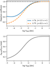 |
Fig. 8 Comparison between LTE and NLTE level and total number density. Top panel: departure coefficients for upper level of the transition A2 ∆ with E = 3.2eV, J = 1.5, and υ = 1 and the lower level X2Π with E = 0.3 eV, J = 0.5, and υ = 1. The dashed black line indicates the departure coefficient for a thermalised level, for which |
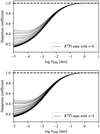 |
Fig. 9 Departure coefficients of levels in ground state X2Π with vibrational quantum number υ = 0 (top) and υ = 5 (bottom), respectively. |
3.2 Metal-poor stars
The spectral features of the CH molecule are usually used for carbon abundance determinations in metal-poor stars (e.g. Aoki et al. 2007; Hansen et al. 2016a; Yoon et al. 2016; Spite et al. 2013). In the following, we discuss the NLTE corrections computed using the model atmospheres described in Sect. 2.3. The results are presented in Table 1. For each such estimate, we also provided a line-to-line scatter that represents the differences in NLTE corrections for individual spectral lines within the G band.
The variation of NLTE abundance corrections with metallicity is shown in Fig. 10. As emphasised earlier, here we focused on the parameters representative of the atmospheres of red giants, as many of them at low metallicity exhibit strong G bands that are used as diagnostics of C abundances. Here, the [C/Fe] ratio was assumed to be scaled solar, but we also explored the dependence of NLTE effects on the assumed C abundance, as shown in the next section. Figure 10 clearly shows that the NLTE abundance corrections increase with decreasing metallicity. For the model atmosphere with the solar metallicity, the NLTE corrections are, on average, around ΔNLTE = +0.12 ± 0.02 dex. However, the NLTE correction increases to around +0.2 dex at [Fe/H] = −4.0.
Our results thus suggest that standard LTE analyses of the CH molecular lines in spectra of RGB stars under-estimate the abundance of C, and the bias is inversely proportional to metallicity, in the sense that NLTE effects are larger and more positive for lower metallicity red giants.
NLTE abundance corrections for stellar model atmospheres with different metallicities [Fe/H] and carbon-to-iron abundance ratios [C/Fe].
 |
Fig. 10 NLTE abundance corrections for model atmospheres with Teff = 4500 K and log g = 2.0 with different metallicities, [Fe/H]. |
 |
Fig. 11 NLTE abundance corrections for metal-poor, carbon-enhanced model atmospheres with metallicities of [Fe/H] = −3.0 and [Fe/H] = −4.0 and carbon-abundance ratios [C/Fe] = 0.0, +0.7, +1.5, and +3.0. |
3.3 Carbon-enhanced metal-poor stars
The NLTE analysis of the CH molecule is particularly important for C-enhanced metal-poor (CEMP) stars (Sect. 1). Especially at low metallicities, the CH molecule exhibits some of the strongest detectable features in the spectra.
The NLTE abundance corrections of the C-enhanced models are displayed in Fig. 11 and also provided in Table 1. Here, we focused on red giants with metallicities [Fe/H] = −3.0 and [Fe/H] = −4.0 and different [C/Fe] ratios ranging from 0 to 3 dex. Generally, the NLTE corrections are not very sensitive to the assumed C abundance. For the most metal-poor model, [Fe/H] = −4.0, the NLTE corrections decrease in amplitude with increasing [C/Fe] ratio. For the model atmosphere with [Fe/H] = −3, the NLTE G-band correction remains at the level of +0.17 dex for all [C/Fe] ratios considered. This implies that some non-carbon-enhanced metal-poor stars may in fact have higher C abundances than determined with LTE models.
Additionally, Fig. 12 shows the NLTE abundance corrections for all individual transitions in the wavelength range 4297–4303 Å, as a function of the lower level of energy, for the models that showed the largest variation in the corrections ([C/Fe] = +0.0, +1.5 dex). For both metallicities the NLTE corrections increase for the transitions with a higher excitation potential, reaching 0.27 dex for the C-enhanced ([C/Fe] = +1.5) model atmosphere with a metallicity of [Fe/H] = −3. The strong dependence on the NLTE corrections on the lower level energy may indicate that the temperature structure inferred from the excitation balance of CH lines may be prone to systematic biases.
4 Discussion
We show that the G band of the CH molecule experiences non-negligible NLTE effects for all the considered model atmospheres of K-type red giant stars apart from the Sun, with the NLTE effects increasing with decreasing metallicity of the model. This finding is important for all previous and future studies that use the spectrum of the CH molecule for carbon-abundance determinations in stellar atmospheres.
Based on these results, when using the spectral features of the CH molecule, the computed LTE carbon abundances for stars with stellar parameters similar to those considered in this work have to be revised, and adjusted by the corresponding NLTE corrections. For example, the determined LTE carbon abundance of a star with Teff = 4500 K, log g = 2.0, [Fe/H] = −3.0, and [C/Fe] = 0.0 would have to be increased by 0.18 dex, which corresponds to a factor of 1.51.
As this is the first attempt at computing the G band of the CH molecule in NLTE, no direct comparison with the literature can be made. The NLTE modelling of molecular bands is a quite recent field of research, and has not been attempted by many, mainly due to the complexities involved in modelling the spectrum of molecules due to the large number of energy levels and lines. An early NLTE analysis was done by Ayres & Wiedemann (1989) for the Δυ = 1 band of the CO molecule in late-type atmospheres. Their model molecule was represented by ten bound vibrational states each split into 121 rotational sub-states, which were connected by 1000 radiative transitions. Their results yielded very small NLTE effects for the Sun, but larger effects for Arcturus. An NLTE analysis of the H2O molecule was carried out by Lambert et al. (2013) in the model atmospheres of red supergiants (RSG). They reported negative NLTE corrections for the H2O lines in the far infra-red (~3 μm) spectrum of the RSG model. The inversion of NLTE effects is not unexpected, because the effects in such lines forming in transitions between high-excitation states are driven by recombination cascades and line scattering. Other species, such as Si, Fe, Mg, and Ti, also show positive NLTE effects in the optical spectra of FGK-type stars, but negative NLTE effects in the spectra of red supergiants (Bergemann et al. 2012, 2013, 2015).
Whereas our NLTE analysis was carried out with 1D hydrostatic model atmospheres, it should be highlighted that effects of 3D convection may also be important in the diagnostic spectroscopy based on molecular lines. A detailed LTE analysis of the G band with 1D and 3D models of a red giant was carried out by Collet et al. (2007). They found that the cooler outermost structures of the 3D models favour a higher concentration of CH molecules, which in turn leads to stronger G-band features and consequently to lower C abundances inferred in 3D, compared to standard modelling with 1D LTE models (see their Table 3). A similar result was reported by Gallagher et al. (2016) for the synthetic G-band in metal-poor dwarfs, where Table 2 of their paper shows that the majority of the 3D corrections are negative. This means that in LTE line formation 1D hydrostatic models overestimate the carbon abundances.
Our results suggest that the NLTE effects in the CH molecule are driven by over-dissociation, owing to the low photo-dissociation threshold of the molecule, and thus the effects will increase with decreasing metallicity and lower density of the model atmospheres. It is therefore not yet clear whether 3D and NLTE effects will compensate for each other, or if an amplification of the effect would result. We therefore caution against co-adding 3D and NLTE corrections, as is sometimes done in the literature. The LTE 1D assumption may indeed predict the correct C abundance, but for the wrong reasons. A detailed quantitative comparison between the 3D and NLTE effects, ideally including full 3D NLTE radiative transfer calculations, is necessary in order to understand which of the effects would dominate the formation of the G-band.
5 Conclusions
In all the previous studies of the CH molecule in the atmospheres of FGK-type stars that we are aware of, the theoretical CH spectral lines were computed using the assumption of LTE. This work presents the first NLTE radiative transfer calculation for the CH molecule under the conditions of metal-poor and carbon-enhanced stellar atmospheres. Our primary aim was to explore the difference between the LTE and the NLTE computation. We focused on the optical G band of the CH molecule, the feature commonly used for C-abundance determinations, especially for cool, metal-poor stars.
Our new NLTE model of the CH molecule included 1981 levels and 53079 radiative transitions adopted from Masseron et al. (2014). The photo-dissociation cross-sections were taken from Kurucz et al. (1987), and collisional reactions were represented by classical semi-empirical recipes such as Regemorter's (van Regemorter 1962) and Allen's formulas (Allen 1973) for collisions with electrons, and Drawin's formula (Steenbock & Holweger 1984) for collisions with H atoms. The detailed statistical equilibrium calculations were performed using the MULTI2.3 code and 1D LTE MARCS model atmospheres.
We find that the G-band NLTE line profiles are systematically weaker compared to their LTE counterparts, regardless of the stellar model atmosphere used. This has a systematic effect on the C-abundance determination. The LTE assumption leads to underestimated C abundances for all considered model atmospheres, by ≈+0.1 dex for solar-metallicity giants and ≈+0.2 dex for metal-poor red giants with [Fe/H] ≲ −3.0. Increasing the [C/Fe] abundance ratio of the model leads to slightly smaller (by ~0.06 dex) NLTE abundance corrections, which may be relevant to studies of CEMP stars.
We also find that, even though the G-band-averaged NLTE corrections are not that large, when inspecting the individual NLTE corrections for the C-enhanced models in Fig. 11, we can see that for some particular lines, especially those arising from transitions with higher energy of the lower level, the NLTE corrections can exceed +0.25 dex. This implies the C abundance would be under-estimated by a factor of 1.8.
The results of this work show that NLTE effects are non-negligible for all considered stellar model atmospheres, suggesting that LTE is not a reliable assumption for the modelling of the CH molecular bands in spectra of cool FGK-type stars.
We note, however, that some important molecular data are still missing. In particular, the collision-induced reactions with electrons and hydrogen atoms require quantum-mechanical treatment, and photo-dissociation cross-sections for higher energy states of the CH molecule are needed. It is also important to mention that we study NLTE effects in the CH molecule in isolation, whereas in reality there are other competing molecules, such as CO, that might affect its abundance and behaviour. Studies of non-equilibrium chemistry with NLTE effects are, however, beyond the scope of the present investigation.
We intend to expand our study to include model atmospheres with larger ranges of effective temperatures and surface gravities so that a more comprehensive set of NLTE corrections can be derived for application to the derivation of [C/Fe] for CEMP stars in the future.
 |
Fig. 12 NLTE abundance corrections for individual G-band lines for model atmospheres with metallicities of [Fe/H] = −3.0 (left) and [Fe/H] = −4.0 (right) for carbon-to-iron ratios [C/Fe] = +0.0, +1.5. |
Acknowledgements
T.C.B. acknowledges partial support for this work from grant PHY 14-30152; Physics Frontier Center/JINA Center for the Evolution of the Elements (JINA-CEE), and OISE-1927130: the International Research Network for Nuclear Astrophysics (IReNA), awarded by the US National Science Foundation. MB is supported through the Lise Meitner grant from the Max Planck Society. We acknowledge support by the Collaborative Research centre SFB 881 (projects A5, A10), Heidelberg University, of the Deutsche Forschungsgemeinschaft (DFG, German Research Foundation). This project has received funding from the European Research Council (ERC) under the European Union's Horizon 2020 research and innovation programme (Grant agreement no. 949173).
References
- Abate, C., Pols, O. R., Karakas, A. I., & Izzard, R. G. 2015, A&A, 576, A118 [NASA ADS] [CrossRef] [EDP Sciences] [Google Scholar]
- Allen, C. W. 1973, Astrophysical Quantities (Athlone Press) [Google Scholar]
- Aoki, W., Beers, T. C., Christlieb, N., et al. 2007, ApJ, 655, 492 [NASA ADS] [CrossRef] [Google Scholar]
- Aoki, W., Beers, T. C., Sivarani, T., et al. 2008, ApJ, 678, 1351 [Google Scholar]
- Aoki, W., Beers, T. C., Honda, S., et al. 2022, PASJ, 74, 273 [NASA ADS] [CrossRef] [Google Scholar]
- Asplund, M., Nicolas, G., Sauval, A., & Scott, P. 2009, ARA&A, 47 [Google Scholar]
- Ayres, T. R., & Wiedemann, G. R. 1989, ApJ, 338, 1033 [NASA ADS] [CrossRef] [Google Scholar]
- Barklem, P. S. 2016, A&AR, 24, 9 [NASA ADS] [CrossRef] [Google Scholar]
- Bautista, M. A., Bergemann, M., Gallego, H. C., et al. 2022, A&A, 665, A18 [NASA ADS] [CrossRef] [EDP Sciences] [Google Scholar]
- Beers, T. C., & Christlieb, N. 2005, ARA&A, 43, 531 [NASA ADS] [CrossRef] [Google Scholar]
- Beers, T. C., Carollo, D., Ivezić, Ž., et al. 2012, ApJ, 746, 34 [NASA ADS] [CrossRef] [Google Scholar]
- Bergemann, M., & Nordlander, T. 2014, ArXiv e-prints [arXiv:1403.3088] [Google Scholar]
- Bergemann, M., Kudritzki, R.-P., Plez, B., et al. 2012, ApJ, 751, 156 [Google Scholar]
- Bergemann, M., Kudritzki, R.-P., Würl, M., et al. 2013, ApJ, 764, 115 [NASA ADS] [CrossRef] [Google Scholar]
- Bergemann, M., Kudritzki, R.-P., Gazak, Z., Davies, B., & Plez, B. 2015, ApJ, 804, 113 [NASA ADS] [CrossRef] [Google Scholar]
- Bergemann, M., Gallagher, A. J., Eitner, P., et al. 2019, A&A, 631, A80 [NASA ADS] [CrossRef] [EDP Sciences] [Google Scholar]
- Bergemann, M., Hoppe, R., Semenova, E., et al. 2021, MNRAS, 508, 2236 [NASA ADS] [CrossRef] [Google Scholar]
- Caffau, E., Monaco, L., Bonifacio, P., et al. 2019, A&A, 628, A46 [NASA ADS] [CrossRef] [EDP Sciences] [Google Scholar]
- Carlsson, M. 1986, Uppsala Astronomical Observatory Reports, 33 [Google Scholar]
- Carollo, D., Beers, T. C., Lee, Y. S., et al. 2007, Nature, 450, 1020 [NASA ADS] [CrossRef] [Google Scholar]
- Carollo, D., Beers, T. C., Chiba, M., et al. 2010, ApJ, 712, 692 [NASA ADS] [CrossRef] [Google Scholar]
- Choplin, A., & Hirschi, R. 2020, J. Phys. Conf. Ser., 1668, 012006 [NASA ADS] [CrossRef] [Google Scholar]
- Choplin, A., Hirschi, R., Meynet, G., & Ekström, S. 2017, A&A, 607, A3 [NASA ADS] [CrossRef] [EDP Sciences] [Google Scholar]
- Collet, R., Asplund, M., & Trampedach, R. 2007, A&A, 469, 687 [NASA ADS] [CrossRef] [EDP Sciences] [Google Scholar]
- Dagdigian, P. J. 2017, J. Chem. Phys., 146, 224308 [NASA ADS] [CrossRef] [Google Scholar]
- Demtroeder. 2003, Atoms, Molecules and Photons [Google Scholar]
- Eugène-Praderie, F., & Pecker, J. C. 1960, Ann. Astrophys., 23, 622 [Google Scholar]
- François, P., Caffau, E., Wanajo, S., et al. 2018, A&A, 619, A10 [Google Scholar]
- Frebel, A. 2018, Annu. Rev. Nucl. Part. Sci., 68, 237 [NASA ADS] [CrossRef] [Google Scholar]
- Frebel, A., & Norris, J. 2015, Annu. Rev. Astron. Astrophys., 53 [Google Scholar]
- Gallagher, A. J., Caffau, E., Bonifacio, P., et al. 2016, A&A, 593, A48 [NASA ADS] [CrossRef] [EDP Sciences] [Google Scholar]
- Gerber, J. M., Magg, E., Plez, B., et al. 2022, Non-LTE Radiative Transfer with Turbospectrum [Google Scholar]
- Gil-Pons, Doherty, C. L., Gutiérrez, J., et al. 2021, A&A, 645, A10 [NASA ADS] [CrossRef] [EDP Sciences] [Google Scholar]
- Goswami, P. P., Rathour, R. S., & Goswami, A. 2021, A&A, 649, A49 [NASA ADS] [CrossRef] [EDP Sciences] [Google Scholar]
- Gustafsson, B., Edvardsson, B., Eriksson, K., et al. 2008, A&A, 486, 951 [NASA ADS] [CrossRef] [EDP Sciences] [Google Scholar]
- Hansen, C. J., Nordström, B., Bonifacio, P., et al. 2011, A&A, 527, A65 [NASA ADS] [CrossRef] [EDP Sciences] [Google Scholar]
- Hansen, C. J., Nordström, B., Hansen, T. T., et al. 2016a, A&A, 588, A37 [NASA ADS] [CrossRef] [EDP Sciences] [Google Scholar]
- Hansen, T. T., Andersen, J., Nordström, B., et al. 2016b, A&A, 588, A3 [NASA ADS] [CrossRef] [EDP Sciences] [Google Scholar]
- Hansen, T. T., Andersen, J., Nordström, B., et al. 2016c, A&A, 586, A160 [NASA ADS] [CrossRef] [EDP Sciences] [Google Scholar]
- Hansen, C. J., Hansen, T. T., Koch, A., et al. 2019, A&A, 623, A128 [NASA ADS] [CrossRef] [EDP Sciences] [Google Scholar]
- Henyey, L., Vardya, M. S., & Bodenheimer, P. 1965, ApJ, 142, 841 [Google Scholar]
- Herzberg, G., & Johns, J. W. C. 1969, ApJ, 158, 399 [NASA ADS] [CrossRef] [Google Scholar]
- Hinkle, K. H., & Lambert, D. L. 1975, MNRAS, 170, 447 [NASA ADS] [Google Scholar]
- Hubeny, I., & Mihalas, D. 2014, Theory of Stellar Atmospheres [Google Scholar]
- Ito, H., Aoki, W., Beers, T. C., et al. 2013, ApJ, 773, 33 [Google Scholar]
- Klessen, R. S., Glover, S. C. O., & Clark, P. C. 2012, MNRAS, 421, 3217 [NASA ADS] [CrossRef] [Google Scholar]
- Kurucz, van Dishoeck, & Tarafdar. 1987, ApJ, 322, 992 [NASA ADS] [CrossRef] [Google Scholar]
- Lambert, J., Josselin, E., Ryde, N., & Faure, A. 2013, in EAS Publications Series, 60, EAS Publications Series, eds. P. Kervella, T. Le Bertre, & G. Perrin, 111 [NASA ADS] [CrossRef] [EDP Sciences] [Google Scholar]
- Lee, Y. S., Beers, T. C., Masseron, T., et al. 2013, AJ, 146, 132 [Google Scholar]
- Liu, B., Sibony, Y., Meynet, G., & Bromm, V. 2021, MNRAS, 506, 5247 [NASA ADS] [CrossRef] [Google Scholar]
- Magg, E., Bergemann, M., Serenelli, A., et al. 2022, A&A, 661, A140 [NASA ADS] [CrossRef] [EDP Sciences] [Google Scholar]
- Masseron, T., Plez, B., Van Eck, S., et al. 2014, A&A, 571, A47 [NASA ADS] [CrossRef] [EDP Sciences] [Google Scholar]
- Meynet, G., Ekström, S., & Maeder, A. 2006, A&A, 447, 623 [NASA ADS] [CrossRef] [EDP Sciences] [Google Scholar]
- Morgan, W. W., Keenan, P. C., & Kellman, E. 1943, An Atlas of Stellar Spectra, with an Outline of Spectral Classification [Google Scholar]
- Nomoto, K., Kobayashi, C., & Tominaga, N. 2013, ARA&A, 51, 457 [CrossRef] [Google Scholar]
- Norris, J. E., & Yong, D. 2019, ApJ [Google Scholar]
- Placco, V. M., Frebel, A., Beers, T. C., et al. 2013, ApJ, 770, 104 [Google Scholar]
- Placco, V. M., Beers, T. C., Reggiani, H., & Meléndez, J. 2016, ApJ, 829, L24 [Google Scholar]
- Plez, B. 2012, Turbospectrum: Code for Spectral Synthesis, Astrophysics Source Code Library, [record ascl:1205.004] [Google Scholar]
- Qian, Y.-Z. 2022, EPJ Web Conf., 260, 09001 [NASA ADS] [CrossRef] [EDP Sciences] [Google Scholar]
- Rasmussen, K. C., Zepeda, J., Beers, T. C., et al. 2020, ApJ, 905, 20 [NASA ADS] [CrossRef] [Google Scholar]
- Ryan, S. G., Aoki, W., Norris, J. E., & Beers, T. C. 2005, ApJ, 635, 349 [NASA ADS] [CrossRef] [Google Scholar]
- Scharmer, G., & Carlsson, M. 1985, J. Comput. Phys., 59, 56 [NASA ADS] [CrossRef] [Google Scholar]
- Spite, M., Caffau, E., Bonifacio, P., et al. 2013, A&A, 552, A107 [NASA ADS] [CrossRef] [EDP Sciences] [Google Scholar]
- Starkenburg, E., Shetrone, M. D., McConnachie, A. W., & Venn, K. A. 2014, MNRAS, 441, 1217 [Google Scholar]
- Steenbock, W., & Holweger, H. 1984, A&A, 130, 319 [NASA ADS] [Google Scholar]
- Tsuji, T. 1973, A&A, 23, 411 [NASA ADS] [Google Scholar]
- van Regemorter, H. 1962, ApJ, 136, 906 [NASA ADS] [CrossRef] [Google Scholar]
- Yong, D., Norris, J. E., Bessell, M. S., et al. 2013, ApJ, 762, 26 [Google Scholar]
- Yoon, J., Beers, T. C., Placco, V. M., et al. 2016, ApJ, 833, 20 [Google Scholar]
- Yoon, J., Beers, T. C., Dietz, S., et al. 2018, ApJ, 861, 146 [NASA ADS] [CrossRef] [Google Scholar]
- Zepeda, J., Beers, T. C., Placco, V. M., et al. 2022a, AAS J., submitted [arXiv:2209.12224] [Google Scholar]
- Zepeda, J., Rasmussen, K. C., Beers, T. C., et al. 2022b, ApJ, 927, 13 [NASA ADS] [CrossRef] [Google Scholar]
All Tables
NLTE abundance corrections for stellar model atmospheres with different metallicities [Fe/H] and carbon-to-iron abundance ratios [C/Fe].
All Figures
 |
Fig. 1 Properties of the transitions in the CH molecule model. Top panel: distribution of line strengths in the entire CH system. Only transitions with strengths greater than S = –5 were included in the NLTE model molecule. Bottom panel: X–A spectrum of the CH molecule around the wavelength of ~4300 Å. The P, Q, and R branches are indicated. The strongest feature in this range, corresponding to J′ − J″ = 0 (vibrational transition accompanied by a rotational transition) is the astrophysically famous 'G band'. |
| In the text | |
 |
Fig. 2 Energy levels included in CH molecule model with specified rotational quantum number J and vibrational quantum number υ. The black lines indicate the bound-bound transitions between the electronic states A2Δ and X2Π that give rise to the molecular G-band lines in the wavelength 4297–4303 Å range. |
| In the text | |
 |
Fig. 3 Energy levels included in the CH molecule model with specified rotational quantum number J and vibrational quantum number υ. The black lines indicate all radiative bound-bound transitions included in the model. |
| In the text | |
 |
Fig. 4 Black lines indicate the transitions for the photo-dissociation reactions with the dissociation energy of 3.45 eV. |
| In the text | |
 |
Fig. 5 Cross-section distribution of photo-dissociation for energy level at 2.45 eV (19777.31 cm−1) with the following configuration: electronic state X2Π with quantum numbers υ = 0 and J = 40. |
| In the text | |
 |
Fig. 6 LTE and NLTE spectra in region of CH G band, computed using the model atmosphere with a solar carbon abundance of A(C) = 8.43. |
| In the text | |
 |
Fig. 7 LTE and NLTE line proflies of the representative G-band line at 4299.48 Å. |
| In the text | |
 |
Fig. 8 Comparison between LTE and NLTE level and total number density. Top panel: departure coefficients for upper level of the transition A2 ∆ with E = 3.2eV, J = 1.5, and υ = 1 and the lower level X2Π with E = 0.3 eV, J = 0.5, and υ = 1. The dashed black line indicates the departure coefficient for a thermalised level, for which |
| In the text | |
 |
Fig. 9 Departure coefficients of levels in ground state X2Π with vibrational quantum number υ = 0 (top) and υ = 5 (bottom), respectively. |
| In the text | |
 |
Fig. 10 NLTE abundance corrections for model atmospheres with Teff = 4500 K and log g = 2.0 with different metallicities, [Fe/H]. |
| In the text | |
 |
Fig. 11 NLTE abundance corrections for metal-poor, carbon-enhanced model atmospheres with metallicities of [Fe/H] = −3.0 and [Fe/H] = −4.0 and carbon-abundance ratios [C/Fe] = 0.0, +0.7, +1.5, and +3.0. |
| In the text | |
 |
Fig. 12 NLTE abundance corrections for individual G-band lines for model atmospheres with metallicities of [Fe/H] = −3.0 (left) and [Fe/H] = −4.0 (right) for carbon-to-iron ratios [C/Fe] = +0.0, +1.5. |
| In the text | |
Current usage metrics show cumulative count of Article Views (full-text article views including HTML views, PDF and ePub downloads, according to the available data) and Abstracts Views on Vision4Press platform.
Data correspond to usage on the plateform after 2015. The current usage metrics is available 48-96 hours after online publication and is updated daily on week days.
Initial download of the metrics may take a while.


