| Issue |
A&A
Volume 670, February 2023
|
|
|---|---|---|
| Article Number | A12 | |
| Number of page(s) | 15 | |
| Section | Interstellar and circumstellar matter | |
| DOI | https://doi.org/10.1051/0004-6361/202244227 | |
| Published online | 31 January 2023 | |
Disentangling the protoplanetary disk gas mass and carbon depletion through combined atomic and molecular tracers★
1
Leiden Observatory, Leiden University,
PO Box 9513,
2300 RA
Leiden, The Netherlands
e-mail: This email address is being protected from spambots. You need JavaScript enabled to view it.
2
European Southern Observatory,
Karl-Schwarzschild-Strasse 2,
85748
Garching bei München, Germany
Received:
9
June
2022
Accepted:
16
September
2022
Abstract
Context. The total disk gas mass and elemental C, N, and O composition of protoplanetary disks are crucial ingredients for improving our understanding of planetary formation. Measuring the gas mass is complicated, since H2 cannot be detected in the cold bulk of the disk and the elemental abundances with respect to hydrogen are degenerate with gas mass in all disk models.
Aims. We aim to determine the gas mass and elemental abundances ratios C/H and O/H in the transition disk around LkCa 15, one of the few disks for which HD data are available, in combination with as many chemical tracers as possible.
Methods. We present new NOrthern Extended Millimeter Array observations of CO, 13CO, C18O, and optically thin C17O J = 2−1 lines, along with high angular-resolution Atacama Large Millimeter Array millimeter continuum and CO data to construct a representative model of LkCa 15. Using a grid of 60 azimuthally symmetric thermo-chemical DALI disk models, we translated the observed fluxes to elemental abundances and constrained the best-fitting parameter space of the disk gas mass.
Results. The transitions that constrain the gas mass and carbon abundance the most are C17O J = 2−1, N2H+ J = 3−2 and HD J = 1−0. Using these three molecules, we find that the gas mass in the LkCa 15 disk is Mg = 0.01−0.004+0.01 M⊙, which is a factor of 6 lower than previous estimations. This value is consistent with cosmic ray ionization rates between 10−16−10−18 s−1, where 10−18 s−1 is a lower limit based on the HD upper limit. The carbon abundance is C/H = (3 ± 1.5) × 10−5, implying a moderate depletion of elemental carbon by a factor of 3–9. All other analyzed transitions also agree with these numbers, within a modeling uncertainty of a factor of 2. Using the resolved C2H image we find a C/O ratio of ~1, which is consistent with literature values of H2O depletion in this disk. The absence of severe carbon depletion in the LkCa 15 disk is consistent with the young age of the disk, but stands in contrast to the higher levels of depletion seen in older cold transition disks.
Conclusions. Combining optically thin CO isotopologue lines with N2H+ is promising with regard to breaking the degeneracy between gas mass and CO abundance. The moderate level of depletion for this source with a cold, but young disk, suggests that long carbon transformation timescales contribute to the evolutionary trend seen in the level of carbon depletion among disk populations, rather than evolving temperature effects and presence of dust traps alone. HD observations remain important for determining the disk’s gas mass.
Key words: protoplanetary disks / astrochemistry / planets and satellites: formation
The reduced moment zero images and the integrated spectra are only available at the CDS via anonymous ftp to cdsarc.cds.unistra.fr (130.79.128.5) or via https://cdsarc.cds.unistra.fr/viz-bin/cat/J/A+A/670/A12
© The Authors 2023
 Open Access article, published by EDP Sciences, under the terms of the Creative Commons Attribution License (https://creativecommons.org/licenses/by/4.0), which permits unrestricted use, distribution, and reproduction in any medium, provided the original work is properly cited.
This article is published in open access under the Subscribe-to-Open model. This email address is being protected from spambots. You need JavaScript enabled to view it. to support open access publication.
1 Introduction
The total mass of a protoplanetary disk is one of its most significant properties. The disk mass sets the potential for planet formation at different evolutionary stages and it is a fundamental input for models of the disk chemical inventory, planetary formation, and planet-disk interactions (see e.g., Lissauer & Stevenson 2007; Mordasini et al. 2012). In contrast to the dust mass, which can be relatively well constrained by the spectral energy distribution and resolved mm continuum observations (Hildebrand 1983), the gas mass is much harder to determine. Over 99% of the gas resides in H2 and He, which cannot be directly observed in the bulk of the disk due to lack of a dipole moment. Hydrogen deuteride (HD) is emitted from the warmer atmospheric layers in the disk and can be used to determine the gas mass within a factor of a 2 (Favre et al. 2013; McClure et al. 2016; Trapman et al. 2017). However, only a handful of the most massive sources have obtained a detection of the HD 1–0 line, using far-infrared Herschel observations (Bergin et al. 2013; McClure et al. 2016), and unless a far-infrared facility is selected for NASA’s upcoming probe class mission, no instruments will be able to target HD in the near future. For several massive disks, Herschel HD upper limits can provide additional constraints on the gas mass (Kama et al. 2020).
Carbon monoxide (CO), the second most abundant molecule in disks, is often used to trace the disk mass using a scaling factor to find the total gas mass. Early studies of a few disks have found unexpectedly weak CO emission (van Zadelhoff et al. 2001; Dutrey et al. 2003; Chapillon et al. 2008; Favre et al. 2013). Recent large surveys in the nearby low-mass star-forming regions Lupus and Chamaeleon (Ansdell et al. 2016, 2018; Long et al. 2017; Miotello et al. 2017) have suggested that weak CO emission is common and that CO might be one to two orders of magnitude less abundant in protoplanetary disks than the canonical interstellar medium (ISM) value of C/H = 1.35 × 10⁻⁴. This depletion is greater than the amount of depletion expected purely from freeze-out and photo-dissociation. Carbon monoxide is thought to be stored in ices on large dust grains in the midplane and out of reach of chemical equilibrium, which could result in low elemental C/H and O/H abundances in the gas, as compared to the ISM value (see e.g., Kama et al. 2016b; Sturm et al. 2022). These elemental ratios are very important for the disk chemistry and understanding the mechanisms that set these values is crucial for understanding the formation of habitable planets.
Assessing the degree of CO depletion is complicated by several factors. First, CO depletion is thought to be a combination of dust grain growth, radial and vertical dust dynamics, CO freeze-out, and the chemical processing of CO (van Zadelhoff et al. 2001; Williams & Best 2014; Miotello et al. 2017; Booth et al. 2017; Schwarz et al. 2018; Bosman et al. 2018; Krijt et al. 2018, 2020; Zhang et al. 2019). Second, recent studies that observed the rare isotopologues 13C18O (Zhang et al. 2020a) and 13C17O (Booth et al. 2019) show that even C18O lines can be optically thick in the densest, innermost regions of the disk, attributed to enhanced abundances due to radial drift of ice rich material on large dust grains within the snowline. Third, the C/O ratio in the gas is thought to be radially varying between 1 at large radii and ~0.47 at small radii because of the freeze-out of key C and O bearing species such as H2O, CO and CO2 (Öberg et al. 2011a; Eistrup et al. 2016). Additional elevation is inferred in a number of disks by the strong lines of small carbon chains such as C2H and C3H2 that require C/O ratios of 1.5–2 to form efficiently (Bergin et al. 2016; Miotello et al. 2019; Bergner et al. 2019; Ilee et al. 2021; Bosman et al. 2021a). The elevated C/O ratio could be a result of the observed gas phase depletion of H2O and CO2 (Bergin et al. 2010; Hogerheijde et al. 2011; Du et al. 2017; Bosman et al. 2017). Potentially direct photo-ablation of carbon rich grains can also contribute (Bosman et al. 2021b). The C/O ratio in the planetary birth environment is one of the key ingredients in models of planetary atmospheres. A slight increase in C/O ratio in a typical hot Jupiter atmosphere changes abundances of key carbon-bearing species such as CH4 and C2H2 by multiple orders of magnitude (Lodders 2010; Madhusudhan 2019).
Nitrogen bearing molecules are proposed to be good candidate gas mass tracers, since the main molecular carrier of N, N2, has such a low freeze-out temperature that the depletion of nitrogen is likely to be less severe than that of oxygen and carbon (Tafalla & Santiago 2004; Cleeves et al. 2018; Visser et al. 2018). A smaller fraction of the total amount of nitrogen is contained in meteorites and comets, which suggests that less material is depleted from the gas phase by freeze-out and further processing on the grains (see more details in Bergin et al. 2015; Anderson et al. 2019). Since N2 cannot be observed directly under typical disk conditions by lack of a dipole moment, much less abundant species such as HCN, CN, and N2H+ are necessary for probing the disk mass. However, most of these molecular abundances are dependent on the C/H abundance in the disk. As for N2H+, which is observed in a large number of disks (Öberg et al. 2010, 2011b; 2019), it is the most promising candidate as it does not contain a carbon atom, but it is destroyed by proton transfer in the vicinity of gaseous CO (van’t Hoff et al. 2017; Anderson et al. 2019). Anderson et al. (2019, 2022) have shown, based on a small survey of N2H+ emission lines, that N2H+ can be used in combination with C18O to constrain the carbon abundance and total gas mass, which was confirmed in the recent modeling work of Trapman et al. (2022), comparing the outcome with established HD modeling. No single molecule is an optimum tracer, but here we investigate whether a combination of these molecules would work best to disentangle the gas mass from the elemental abundance determination.
This paper is organized as follows. In Sects. 2 and 3, we present the object of study, LkCa 15, along with previous works on measuring the gas mass in this system and new findings. Section 4 summarizes the physical-chemical modeling framework. In Sect. 5, we compare the results of a range of possible modeling parameters with the data. In Sect. 6, we discuss the results and present our conclusions.
2 Observations
2.1 The LkCa 15 disk
In this paper, we focus on one specific source, LkCa 15, which is one of the few disks for which observations in many gas mass tracers exist, including an HD upper limit. Comparing multiple proposed gas mass tracers and the C/O ratio tracer C2H, we aim to constrain the gas mass and C/H and O/H abundances in the bulk of the disk. LkCa 15 is a relatively young (~2 Myr old Andrews et al. 2018) T Tauri star located at a distance of 157.2 pc, as determined by Gaia (Gaia Collaboration 2016, 2021) in the Taurus star forming region (see Table 1 for details). It has a well-studied transition disk, with a dust disk cavity of ~50–65 AU, where the millimeter sized dust grains are depleted (e.g., Piétu et al. 2006; Isella et al. 2012; Facchini et al. 2020). Most of the millimeter dust continuum is emitted from two bright rings between 50 and 150 AU. Micron-sized dust grains are observed in scattered light observations in an inner disk inside the dust gap up to ~30 AU (Oh et al. 2016; Thalmann et al. 2016). Spatial segregation in dust sizes supports the presence of a massive planet orbiting at ~40 AU (Pinilla et al. 2012; Facchini et al. 2020). There has been speculation about the existence of multiple planets inside the cavity based on asymmetric emission in scattered light and Ha emission (Kraus & Ireland 2012; Sallum et al. 2015), but these were later shown to be likely due to disk features (Thalmann et al. 2016; Currie et al. 2019). The gas disk extends out to ~1000 AU (Jin et al. 2019) and has a significantly smaller cavity than the one found in the dust at 15–40 AU (van der Marel et al. 2015; Jin et al. 2019; Leemker et al. 2022).
Previous estimates of the mass in the LkCa 15 disk were based on the SED and the millimeter dust continuum (~0.06 M⊙ Isella et al. 2012; van der Marel et al. 2015; Facchini et al. 2020) and a combination of the SED and the upper limit from the HD 1–0 line, which gives 0.062 M⊙ (McClure et al. 2016). Jin et al. (2019) used optically thick CO and 13CO lines and the assumption of a gas-to-dust ratio of 1000 and a constant CO/H2 abundance of 1.4 × 10⁻⁴ to find a gas mass of ~0.1 M⊙. Facchini et al. (2020) found an upper limit of the gas-to-dust ratio using stability arguments against gravitational collapse of 62 and 68 in the two bright dust continuum rings, respectively, containing the bulk of the total dust mass.
2.2 Observational details
We present new NOEMA (NOrthern Extended Millimeter Array) observations targeting the optically thin 13C18O and C17O J = 2−1 lines, 13CO, C18O, and CN. These new NOEMA observations combined with a large number of high-resolution archival ALMA CO isotopologue observations, N2H+ and C2H emission, and a HD upper limit allow us to study the possible gas mass range and composition of LkCa15 in much more detail, breaking the degeneracy between the disk gas mass and C/H and O/H abundances.
The new NOEMA observations were taken on the 26 and 27 of November 2020. All nine antennae were used with baselines ranging from 32 to 344 m. Three calibrators were used, 0507+179, LKHA101, and 3C84 to correct, respectively, the phase, amplitude, and flux and radio interference. We integrated for 7.5 h on-source, resulting in a sensitivity of 40 mJy/Beam at a velocity resolution of 0.2 km s−1. Imaging was done using CASA v5.4.0. (McMullin et al. 2007) using Briggs weighting and a robust factor of 0.5. The resolution of the final images is typically 1.1″ × 0.7″ or ~150 AU at the distance of LkCa 15. Observational details are given in Table 2.
Additionally, this project makes use of data from various archival ALMA programs, which are summarized in Table 2. We include high-resolution CO J = 2−1, 13CO J = 2−1 and C18O J = 2−1 lines to constrain the radial profile of the CO emission, 13CO J = 6−5 to further constrain the temperature profile (Leemker et al. 2022), and C2H to constrain the C/O ratio in the disk. CO isotopologue ALMA data were self-calibrated in CASA and CLEANed using a Keplerian mask. Further details of the data and initial calibration are described in Leemker et al. (2022). C2H ALMA observations and reduction are described in more detail in Bergner et al. (2019). N2H+ observations are described in Qi et al. (2019), and are consistent with those reported in Loomis et al. (2020). The upper limit for HD J = 1−0 is taken at 3σ from Herschel data (McClure et al. 2016). The properties of all emission lines and an overview of the observations are presented in Table 2.
LkCa 15 source properties.
2.3 Data analysis
Integrated emission or moment 0 maps were created for all NOEMA lines and CO isotopologue ALMA data by integrating over the emission inside the same Keplerian mask that is used in the CLEANing process, set by the source parameters given in Table 1 and restricted to ±4 km s−1 from the source velocity. The moment 0 maps are presented in Fig. 1, together with the 12CO J = 2−1 and continuum images of the ALMA Band 6 data for comparison. Integrated line fluxes are determined using a mask extending to 6.5″ or ~1000 AU in radius and are presented in Table 2 and are shown in black in the right panel of Fig. 2.
All moment 0 maps are deprojected and averaged along azimuth using the geometrical source properties given in Table 1. We chose the source center for each molecule as the pixel (typically 1/5 of the beam) with the peak flux or, in case the cavity is resolved, the pixel with the lowest flux inside the cavity. The source center is shifted with maximum 0.1″ from the reference position, which is a result of the observed eccentric inner disk (Thalmann et al. 2016; Oh et al. 2016), the high inclination (55°) of the main disk and the different observing dates. The radial profiles are presented in Fig. 2 as black lines, the 1 σ uncertainty is masked around the curves. We include the radial profile of the C2H emission from Bergner et al. (2019) and the N2H+ from (Qi et al. 2019). The radial profile of the continuum from Facchini et al. (2020) is included in Fig. 3.
3 Observational results
All targeted CO isotopologues, except for 13C18O J = 2−1, were detected. The spectra of all detected emission lines are presented in the top panel of Fig. 1. Here, C17O J = 2−1 is robustly detected with NOEMA at a S/N of 6. The 13C18O J = 2−1 line is not detected so we listed the 3σ upper limit in Table 2. The upper limit for 13C18O results in a minimum C17O/13C18O ratio of 4.6, compared with the elemental abundance ratio of 24. The observed 13CO and C18O J = 2−1 disk integrated fluxes in the NOEMA and ALMA observations agree well with each other. In addition we detect 8 hyper-fine CN N = 2−1 lines that we combine into one single image. Based on the ratio of the hyper-fine lines we find that the emission is optically thick for the blended lines at 226.87 GHz and 226.66 GHz, but optically thin for the other lines.
Most of the observed CO isotopologue lines are centrally peaked, without resolving the inner cavity. The inner cavity is resolved in the 13CO J = 2−1 and C18O J = 2−1 ALMA data, lately confirmed by Leemker et al. (2022) using 13CO J = 2−1 data with higher spatial resolution and using the high velocity line wings that trace regions closer in to the star than the spatial resolution of the data (Bosman et al. 2021c). The CN emission is centrally peaked and extends out to 1000 AU, similar to the 12CO data.
4 Modeling framework
Our aim is to distentangle the gas mass and elemental abundances C/H and O/H in LkCa 15. For that purpose we made a representative model of LkCa 15 using the azimuthally symmetric physical–chemical model Dust And LInes DALI (DALI; Bruderer et al. 2012; Bruderer 2013). To find the best representative geometry, density structure, and composition of the LkCa 15 disk, we combined information from the spectral energy distribution (SED), high-resolution ALMA continuum observations, the emission lines discussed in Sect. 2.2 and observables from scattered light observations, as well as near-infrared spectra from the Infrared Telescope Facility (IRTF) facility using SpeX (Espaillat et al. 2010).
4.1 Model parameters
The first step in our modeling was to set up a geometrical density structure including all radiation sources that is consistent with the data. For the dust density structure we adopted a fully parametrized surface density profile with a power law surface density dependence on radius (r) and an exponential outer taper:
![Mathematical equation: ${{\rm{\Sigma }}_{{\rm{dust}}}} = {{{{\rm{\Sigma }}_{\rm{c}}}} \over }{\left( {{r \over {{R_c}}}} \right)^{ - \gamma }}\exp \left[ { - {{\left( {{r \over {{R_c}}}} \right)}^{2 - \gamma }}} \right],$](/articles/aa/full_html/2023/02/aa44227-22/aa44227-22-eq5.png) (1)
(1)
where Σc is the surface density at the characteristic radius, Rc, γ the power law index, and ϵ the gas-to-dust ratio. Following the approach of D’Alessio et al. (2006), we split the dust into a small dust population which ranges from 0.005 to 1 μm and a large dust population which includes the small dust sizes, but extends to 1000 μm To calculate the opacities we assume a standard ISM dust composition following Weingartner & Draine (2001), combined using Mie theory, consistent with Andrews et al. (2011). We also included polycyclic aromatic hydrocarbons (PAHs), assumed to be 0.1% of the ISM abundance following Geers et al. (2006). The small dust grains follow an exponential dependence on the height in the disk, given by:
![Mathematical equation: ${\rho _{{\rm{d,small}}}} = {{\left( {1 - {f_\ell }} \right){{\rm{\Sigma }}_{{\rm{dust}}}}} \over {\sqrt {2\pi } rh}}\exp \left[ { - {1 \over 2}{{\left( {{{\pi /2 - \theta } \over h}} \right)}^2}} \right],$](/articles/aa/full_html/2023/02/aa44227-22/aa44227-22-eq6.png) (2)
(2)
where θ is the opening angle from the midplane as seen from the center, h is the scale height defined by h = hc(r/Rc)ψ and fℓ is the mass fraction of large grains. We parametrized dust settling by replacing the scale height of the large grains by χh, so that only a fraction 1 − ft of the grains is distributed throughout the height in the disk. We fixed χ at 0.2 and fℓ at 0.98, adopted from McClure et al. (2016; see also Andrews et al. 2011). The gas surface density follows the same radial and vertical distribution as the small dust grain population, but scaled by the total gas-to-dust ratio, which we take initially at 100. Within the dust sublimation radius, both dust and gas surface density are set to zero. To include a cavity in the dust and gas we scaled the dust and gas surface density profiles independent from each other inside a given radius, Rgap, with respect to the distribution given in Eq. (2) and with constant scaling factors, δd and δg. To account for the three rings observed in the high-resolution continuum images (Facchini et al. 2020), we scaled up the dust density distribution in three intervals (see Fig. 3 for a visualization of the density distribution of the dust and gas).
The stellar spectrum is approximated as a blackbody with temperature Teff = 4730 K. We added an additional UV component to account for gas accretion using a plasma temperature (Tacc) of 10 000 K, with a luminosity given by:
 (3)
(3)
where Bυ (Tacc, υ) is Planck’s law for blackbody radiation, M*. is the stellar mass, R* is the stellar radius and Ṁ the mass accretion rate. We adopted stellar parameters from Espaillat et al. (2010) and Pegues et al. (2020), given in Table 1 resulting in LUV = 0.06 L⊙. We note that the observed values of Ṁ are uncertain up to an order of magnitude and can change over time. We included X-rays assuming an X-ray luminosity of 1030 erg s−1 at a plasma temperature of 7 × 10⁷ K. The cosmic ionization rate incident on the surface of the disk is set to 5 × 10⁻¹⁷ s−1.
Using the sources of radiation and the density structure described in Sect. 4.1, we determined the dust temperature and continuum mean intensity in each grid cell using a Monte-Carlo approach, where photon packages are started randomly from the star, dust grains, or the background.
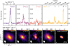 |
Fig. 1 Disk-integrated spectra (top) and total intensity or moment 0 maps of the new emission lines (bottom) obtained with NOEMA at 1.1″ × 0.7″. ALMA band 6 continuum data at 0.3″ × 0.3″ are shown for comparison. Integration limits for the moment 0 maps are indicated with black tickmarks in the bottom at −4 and +4 km s−1. Robustly detected CN hyper-fine structure lines are indicated in the top right panel with black tick marks. For each moment 0 map, the beam is shown as a white ellipse in the lower left corner. |
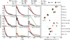 |
Fig. 2 Azimuthally averaged radial proflies of the different gas tracers used in this work (left). Data are shown as black lines with shaded 1 σ uncertainty and normalized to the brightest point for visualization purposes. The full width at half maximum of the beams is shown as a black horizontal line in the lower left-hand corner. The best-fitting model with a gas mass of 0.012 M⊙ and a factor of 4 in carbon depletion is overplotted in red. The blue line shows the same model but with a lower gas-to-dust ratio, resulting in a gas mass of 4 × 10⁻⁴ M⊙, and no carbon depletion. This model reproduces the optically thick CN and CO lines somewhat better, but underproduces the optically thin N2H+ line. The orange line illustrates the C2H radial profile for an increased C/O ratio of 1.1. With C/O > 1 excess carbon, not in CO, changes the carbon chemistry completely. Integrated line flux of the various emission lines analyzed in this paper (right). Black squares represent the observed line fluxes of NOEMA data, black diamonds represent the observed line fluxes of ALMA data, black triangles denote upper limits, taken at 3σ. Colored diamonds show the results for the same models as in the left panel. |
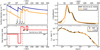 |
Fig. 3 Setup of the DALI model for LkCa 15, top-left: normalized surface density of the dust (orange) and gas (blue) as function of radius, bottom-left: gas-to-dust ratio as function of radius in the fiducial model, this is a direct consequence of the used gas and dust surface density profiles shown in the top left panel, top-right: radial profile of the continuum observations (black) and the model (orange) normalized to 1, bottom-right: observed SED in black with the modeled continuum fluxes in orange. Dashed lines show the setup for the same model with cleared cavity, discussed in Appendix B. |
LkCa 15 line properties.
4.2 Chemical networks
The gas temperature is iteratively solved together with the chemistry, since the gas temperature is dependent on the abundance and excitation of different coolants in the disk. We used two different chemical networks in DALI to cover both the isotope selective processes of CO and proper treatment of C2H and CN. For the CO isotopologue emission we used the HD chemistry described in Trapman et al. (2017), but adapted it to the reduced CO isotopologue network described in Miotello et al. (2016) rather than the full network described in Miotello et al. (2014) to save computation time. This network includes HD, D, HD+, D+, 13CO, C18O, C17O, and 13C18O as separate species, resulting in a total of 189 species and 5789 reactions (compared to 280 species and 9789 reactions in Trapman et al. 2017). For CN and C2H we used the expanded network described in Cazzoletti et al. (2018) and Visser et al. (2018). Nitrogen isotopes are not considered. Reaction types include standard gas-phase reactions, photoionization and -dissociation, X-ray and cosmic ray induced reactions, freeze-out and (non-) thermal desorption, PAH and small grain charge exchange, as well as hydrogenation and reactions with vibrationally excited H2  . Details of these reactions are described in Bruderer et al. (2012), Trapman et al. (2017), and Visser et al. (2018).
We adopted fiducial ISM gas-phase volatile elemental carbon, oxygen, and nitrogen abundances of C/H = 135 ppm, O/H = 288 ppm, and N/H = 21.4 ppm, respectively (Cardelli et al. 1996; Meyer et al. 1998; Parvathi et al. 2012), and 13C, 18O, 17O abundance ratios of 77, 560, and 1792 with respect to their most abundant isotopes (Cardelli et al. 1996; Meyer et al. 1998; Parvathi et al. 2012; Wilson 1999). All volatile carbon, oxygen, and nitrogen starts in atomic form in the gas, but can cycle between gas and ice. The chemistry is run time dependently for 1 Myr. Most line strengths do not change when run in steady-state mode, because the surface layer dominates the abundance of these molecules where the chemistry is fast and emission is not sensitive to the time step.
N2H+ is modeled using a separate, simple chemical network described in van’t Hoff et al. (2017) for a better treatment of the charge distribution. This network focuses specifically on the ionization balance between H3+, N2H+, and HCO+, including freeze-out, thermal desorption, and photodissociation of CO and N2. Using this simplified network has the advantage of being easier to understand the ionization balance, while using the same temperature structure and CO and N2 abundances as in the complete model.
After the chemistry is converged, the model is ray-traced in the analyzed transition lines and at 200 continuum wavelengths from 0.1 to 10 000 μm. Following a similar approach as described in Sect. 2.2, we created moment 0 maps and radial profiles for each of the model lines.
4.3 Modeling approach
Initially we fit the disk parameters by eye in a logical order that we describe in the following sections, so that they converge to a model that best represents the available data. The large number of parameters and the computational time of the models make it impossible to use χ2 fitting or Monte Carlo processes on the whole parameter space. This means that it is not possible to derive formal uncertainties of model parameters and to determine correlations or degeneracies between parameters. The final best fit parameters are summarized in Table 3.
4.3.1 Fitting the dust density distribution
The first step was to find a dust density distribution that agrees well with the data. For that purpose we compared the modeled continuum spectrum with the observed SED and the radial profile of the modeled emission to the radial profile of the high-resolution 1.35 mm continuum data (Facchini et al. 2020). The SED is taken from Andrews et al. (2013) and dereddened using the CCM89 extinction curve (Cardelli et al. 1989) and the observed visible extinction AV = 1.5 (Espaillat et al. 2010). As a starting point we used the model by van der Marel et al. (2015), but updated to the new Gaia DR 3 distances and most recent observations. We first fit the aspect ratio, hc, by matching the model with the observations at the base height of the silicate feature at 10 μm, assuming grain size distributions given in Sect. 4.1. This aspect ratio agrees well with the observed emitting heights of the optically thick CO and 13CO lines (see Fig. 4). Subsequently, we fit the dust gap radius based on the radial profile of the continuum observations, using an inner disk that extends to 35 AU as revealed by scattered light observations (Oh et al. 2016; Thalmann et al. 2016). We then varied the flaring index, ψ, and the dust depletion in the gap, δd, to roughly fit the SED and continuum radial profile. The flaring index is low, ψ = 0.075, consistent with a flat disk. The dust mass is fixed to 5.8 × 10⁻⁴ Μ⊙ based on the lower limit from the continuum observations (Isella et al. 2012). This dust mass agrees well with the slope of the SED beyond 1 mm (see Fig. 3), given the adopted grain size distributions and ISM-like grain composition. We included three rings to account for the observed continuum rings, and varied the height of these to match the radial profile of the continuum observations. The way these dust rings are treated results in a decreased model gas-to-dust ratio in these rings, consistent with the upper limits of 68 and 62 constrained by Facchini et al. (2020). The cavity is not completely empty in our model, to account for the third continuum ring inside the dust cavity observed in the 1.3 mm continuum. Clearing a large cavity from dust between 35 and 63 AU (dashed lines in Fig. 3) does not significantly change the gas temperature structure and has no significant effect on the line emission, as we show in Appendix B (see also the discussion in van der Marel et al. 2015). The parameters of the most representative model are listed in Table 3.
LkCa 15 best-fit model parameters.
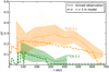 |
Fig. 4 Emitting heights of the 12CO (orange) and 13CO (blue) J = 2−1 emission, taken from Leemker et al. (2022). Scattered points represent the emitting height for each channel, whereas the solid line represents a radially binned average with 1er error. The dashed line shows the height of the τ = 1 line in the DALI model. The disk is flat in both the observations as well as the model. |
4.3.2 Fitting the gas density distribution
The second step in constraining the model is determining the gas density distribution, with γ and Rc constrained by the CO isotopologue lines. For that purpose we ran a grid of models ranging between 50 < Rc < 150 and 0.5 < γ < 4 and took the parameters that reproduced the radial profiles of the CO isotopologue lines the best beyond 200 AU. The gas gap is constrained by high-resolution 13CO and C18O observations with ALMA. The gas surface density inside the gap at 15 AU (~0.1 g cm−1; see Fig. 3) is consistent with upper limits on the total column density determined using C18O (Leemker et al. 2022), but is an order of magnitude higher than the column density upper limit inside 0.3 AU determined from ro-vibrational CO upper limits (Salyk et al. 2009). Lowering the gas surface density in the gap further results in underproducing C17O and 12CO inside the gas gap. We find that LkCa 15 is a large, flat, massive disk with significant structure inside 100 AU in both gas and dust.
We used the C2H flux to determine the C/O ratio in the disk. The elemental carbon depletion and gas mass are then based on the CO isotopologue data, N2H+, CN, and the HD upper limit. To study the degeneracy between the carbon abundance and the gas mass, we run a grid with models for gas-to-dust ratios of [205, 100, 63, 39, 25, 15, 10, 4, 2, 1] and carbon depletion factors [1, 2, 4, 8, 16, 32]. This results in a range of gas masses between 0.1 Μ⊙ and 5×l0−4 Μ⊙. We keep the dust mass fixed at a value of 5.8×l0−4 Μ⊙. We allowed a modeled emission line uncertainty by a factor of 2 to find a confined region where the model is consistent with the data. Confining the region to the model uncertainties circumvents the dependence of the best fit on the S/N of the lines, since the brightest lines (e.g., CO and CN) are not the most sensitive to variations in gas mass and carbon abundance. The choice of a factor of 2 is motivated by an earlier work from Kama et al. (2016a), where the authors varied the most impactful modeling parameters to determine the effect on the total line flux for CO and isotopologues. Also, Bruderer et al. (2012) and Bruderer (2013), in their benchmark of the DALI model, found deviations in flux within a factor of two compared to similar modeling codes due to uncertainties in the reaction rates and desorption temperatures. The geometrical structure of the disk is constrained in this work due to the wealth of data available for LkCa 15. More specific uncertainties and the dependence of the molecular emission flux on important parameters are described in Sect. 6. In Appendix B, we present the result of variations in key parameters and their influence on the total line flux.
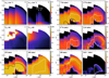 |
Fig. 5 Overview of the DALI model output. The four panels left top (A−D) present the gas and dust density structure and the gas and dust temperature, respectively. The other panels present the molecular abundances of the molecular transitions in the most representative DALI model, assuming a gas-to-dust ratio of 25 and a carbon depletion factor of 4. The white contours represent the region where 95% of the emission originates, the black lines show the τ = 1 surface for the optically thick emission lines. |
5 Results
5.1 Gas distribution
Figure 2 presents the radial profiles and the total fluxes of the best-fitting model. We find that a characteristic radius of Rc = 85 AU and γ = 1.5 fit the emission best at large radii.
5.1.1 HD
The HD 1−0 emission in the model is confined to the inner region <200 AU (see Fig. 5), where the gas temperature is high enough (30–70 K, see also Trapman et al. 2017) to populate the higher levels. This relatively small emitting region is a direct result of the flat geometry of the disk, which means that regions further out in the disk are relatively cool. This makes the total HD 1−0 flux susceptible to temperature variations inside the cavity at 63 AU and changes in the level of gas depletion with respect to the dust.
5.1.2 CO isotopologues
Using the high-resolution CO isotopologue data, we find that the gap inside 35 AU is less depleted in gas than in dust, but a significant gas depletion of a factor of 3 × 10⁻² throughout the cavity is necessary to explain the central dip observed in 13CO and C18O. The inner disk inside 15 AU is depleted further in gas up to a factor 10−3 (see Fig. 3). This is consistent with earlier findings in Leemker et al. (2022); they report a gas cavity size ~15 AU based on the line wings and radial profile of high S/N CO isotopologue data. The two steps in gas depletion (see the top-left panel of Fig. 3) that were necessary to fit the CO lines could be a result of gradual gas depletion inside the cavity.
The best-fitting model reproduces 13CO 2–1, C18O 2–1, C17O 2–1 and 13CO 6–5 within the 1σ error at most radii. The 13CO and C18O emission is predicted to be moderately optically thick in the region just outside the gas cavity, but the C17O emission is optically thin throughout the disk. This is consistent with the observations that show that the disk integrated C18O/C17O ratio of 3.1 is consistent with the expected ISM abundance ratio of 3.2. The models are unable to reproduce the small bump at 500 AU observed in both the C17O and C18O radial profiles (see Fig. 2). This enhancement may be caused by non-thermal desorption processes of CO from the ice due to enhanced UV penetration or a slight change in C/H ratio as a result of infalling pristine material.
The 12CO line is highly optically thick throughout the largest part of the disk (see Fig. 5) and thus primarily sensitive to temperature. Our model reproduces the radial profile of this line and is consistent with the vast size of the disk (see Fig. 2). The 12CO model is somewhat too bright in the outer regions of the disk between 300 and 700 AU, by about a factor of 1.5. The largest recovered angular scale of the 12CO data is r ~600 AU, which likely explains part of the flux that is missing in the outer regions. Changing the geometry (i.e., hc and ψ) does not change the temperature structure sufficiently. The disk is flat (see Fig. 4), and changing hc will only marginally affect the temperature of the highest layers in the disk where the CO and CN emission originate. Lowering the gas mass of the system lowers the height of the emitting layer and results in less flux contribution across the disk, matching the data better. Altering the settling parameters χ or fℓ (see Eq. (2)), as suggested by McClure et al. (2016), changes the temperature in the upper layers and would allow for better fitting of 12CO. However, this results in decreased temperatures that would lead to unrealistically low CO isotopologue fluxes, even with increased values for γ and ISM C/H abundance.
5.1.3 N-bearing species
The N2H+ emission is confined to the inner 300 AU and is in general well reproduced by the model. N2H+ is predominantly formed in regions where the N2 abundance dominates the CO abundance, for example, as a result of differences in their desorption temperature or photo-dissociation rate. Qi et al. (2019) show that the emission can be separated in an extended component, attributed to the small layer between the (vertical) N2 and CO snow surfaces, and an additional ring at ~50 AU due to the difference between the (radial) N2 and CO snowline. The ring at ~50 AU is underproduced in our model (see Fig. 2), which is likely because of the steep temperature gradient just outside the cavity. The difference in desorption temperature between N2 and CO is only 3–7 K (Bisschop et al. 2006) which means that the location of the CO and N2 snowline cannot be determined accurate enough due to the uncertainty in the temperature structure and cavity properties of the system. Using the location of the brightest ring in the N2H+ emission, Qi et al. (2019) find that the midplane CO snowline is located at  AU. This value is consistent with the location of the midplane CO snowline in our model. Assuming a CO freeze-out temperature of 20 K we find that the snowline in our model is located at 66 AU, just outside the cavity. Additional X-ray ionization close to the star, which is not taken into account in our modeling, and a locally decreased CO abundance closer to the snowline (see Krijt et al. 2020) could also partially explain the differences between the observations and our model.
The CN emission is moderately optically thick in some of the hyper-fine structure lines, especially in the strongest blended lines. The best-fitting model roughly follows the shape of the radial distribution (see Fig. 2), but the modeled total flux is too high by nearly a factor of 2. Such a difference is entirely consistent with uncertainties in chemical reaction rate coefficients of the outer disk nitrogen chemistry. Changing the nitrogen abundance in the outer disk does not have a large effect on the CN abundance (see Fig. B.1) and there is no clear physical reason to assume that the nitrogen abundance is lower than the ISM value (see also Bergin et al. 2015). A low gas mass is able to reproduce the CN line, as we show in Fig. 2. Other important parameters have hardly any effect due to the high elevation of the emitting layer in the disk (see Appendix B). The CN emission is located mainly between a height of z/r = 0.2−0.3, higher than the other tracers analyzed in this work.
5.2 Disentangling gas mass and elemental abundances
The gas mass and elemental abundances are interdependent for most tracers. For optically thin CO isotopologues, for example, one determines the total CO mass rather than either the CO abundance or gas mass. To break this degeneracy we ran a grid of 60 models with varying mass and carbon abundance, as described in Sect. 4.3.2. In Fig. 6, we present the integrated line flux of the key molecules for these models with disk gas mass ranging from 0.1 M⊙ − 5×10⁻⁴ M⊙ and system-wide volatile carbon depletion between 1 and 32 with respect to the ISM. We overplot the observed total line fluxes as a dashed white line and colored contours at a factor of 2 for comparison. The colored regions are combined in the main panel for easy comparison of the molecules.
5.2.1 HD
The HD flux is independent of the carbon abundance, as expected, and changes almost directly proportional with the disk gas mass. This indicates that changes in temperature corresponding to the variations in the gas mass do not have strong influence on the emitting region of HD. The observed upper limit of HD constrains the gas mass to be lower than 0.05 M⊙, which gives reliable evidence that the total disk gas mass is lower than expected from the total dust mass (5.8 × 10⁻⁴ M⊙) and the canonical ISM value for the gas-to-dust ratio of 100.
5.2.2 CO isotopologues
C17O has a near-linear relationship between carbon abundance and gas mass, which indicates that the emission is fully determined by the total CO mass in the system. The other CO isotopologue emission lines follow similar trends as C17O, but are slightly less sensitive to changes in gas mass, as these lines are optically thick at least in some parts of the disk. The optically thick 12CO line prefers lower gas masses, for which the emitting surface moves to colder layers deeper inside the disk, decreasing the modeled flux at larger radii (see Sect. 5.1). The total flux of 12CO changes by less than an order of magnitude over the two orders of magnitude in gas mass, which shows that the temperature dependence of the optically thick tracers is much less sensitive to the gas mass than the density dependence of the optically thin tracers.
5.2.3 N-bearing species
We find that the N2H+ emission is strongly dependent on the total gas mass in the system, changing almost in direct proportion with it. N2H+ behaves opposite to CO: it increases in line strength by lower carbon abundances due to less competition with CO for H3+, and less conversion from N2H+ to HCO+ by direct reaction with CO. The CN flux varies by only a factor of ~3 over two orders of magnitude change in gas mass and is roughly independent of the carbon abundance.
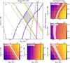 |
Fig. 6 Results of the 10 × 6 model grid with carbon abundance versus disk gas mass. Panel A shows the limits on C/H and Mgas for each emission line, assuming a model uncertainty of a factor of 2. The hashed region denotes the parameter space that matches with all the observed emission lines. Panels B–F show the line flux of key C/H abundance and gas mass tracers N2H+, CN, C17O, HD, and 12CO, respectively, for the same grid of models. The white contours depict the observed flux with observational uncertainty in shaded region. The colored contours mark an average deviation of the model by a factor of 2, the same as in the main panel. The HD observation denotes an upper limit. |
5.2.4 Combining tracers
Without a robust detection of HD, it is not possible to determine either the C/H abundance or the gas mass because all known other tracers vary as function of both quantities. The optically thick tracers CO and CN could in principle be used, but their dependence on the temperature is weak, and the temperature structure is less constrained in the models than the density distribution. However, combining the different tracers (Fig. 6) we find a confined region in the modeling parameter space,  M⊙; C/H = 3 ± 1.5 × 10⁻⁵, that agrees within a factor of 2 with the CO isotopologue fluxes, HD upper limit, CN and N2H+. All optically thin tracers are consistent within the observational uncertainty, assuming the usual 10% calibration error.
5.3 Determination of the C/O ratio
The C2H N = 3−2 transition changes as function of carbon abundance, but is also prone to variations in the C/O ratio. For that reason we leave this species out of the analysis for the carbon abundance in Fig. 6. However, we can use C2H to deduce the C/O ratio in the system and determine the O/H abundance. We find that the integrated line flux of the C2H N = 3−2 transition in our model is not very sensitive to the C/O ratio (see Fig. 2) compared to other sources (see e.g., Bosman et al. 2021a). A change in C/O ratio from ISM level (~0.47) to unity changes the total C2H emission by only a factor of 2, but a little bit of excess carbon, not locked up in CO, (i.e., C/O ratio of 1.1) would make a difference (see Fig. 2) since this changes the carbon chemistry considerably. The bulk of the C2H emission in our model originates from a region at 250−750 AU, that is contributing less prominently in the observed azimuthally averaged radial profile. The maximum resolvable scale of r ~ 600 AU for that data set should be large enough to pick up this emission in the disk. Changing the C/O ratio in the model mainly has an impact on the emission inside 200 AU. With an ISM-like C/O ratio, we underproduce the C2H emission at r < 200 AU with an order of magnitude (see Fig. 2). To determine the C/O ratio, we ran a grid of models varying the C/O ratio by depleting more oxygen in a range between 0.47 and 1.5. This procedure is repeated for a more massive model (green line in Fig. 2). An elevated C/O ratio ~1 matches consistently the centrally peaked emission component, which means that the volatile elemental oxygen abundance in the best-fitting model, 3.4 × 10⁻⁵, is depleted by a factor of 8 with respect to the ISM in the best-fitting model.
6 Discussion
6.1 Comparison with literature gas masses
Previously, the gas mass of LkCa 15 has been inferred from dust continuum observations (Isella et al. 2012), optically thick 12CO and 13CO emission (Jin et al. 2019) and the HD upper limit (McClure et al. 2016). We find with our method a gas mass of  M⊙. This value agrees with the high-resolution continuum observations and observed dust mass, but the total mass of the system is lower than values usually assumed in the literature due to the lower gas-to-dust ratio. We find that the gas mass of LkCa 15 is an order of magnitude lower than the value previously reported in Jin et al. (2019).
There are three key differences between the models described in Jin et al. (2019) and those presented in this work. The first is the assumed density structure in radial and vertical direction. Our models follow the standard formulation for viscous disks with a power law and exponential taper (see Eq. (1)) and a Gaussian vertical distribution (see Eq. (2)). Jin et al. (2019) neglect the exponential taper and solve the hydrostatic equation to find a self-consistent vertical density structure. Neglecting the exponential taper leads to very high values of the power law index; they find γ = 4, compared to our γ = 1.5. They show that using lower values for γ, which reproduces their 13CO emission but not 12CO, leads to values for the gas mass that are consistent with that found in this work.
The second difference is the temperature structure. Jin et al. (2019) mainly analyze the optically thick 12CO 3−2 emission that traces the temperature structure rather than the density structure in the disk, which is much less sensitive to the mass than optically thin tracers (see Fig. 6). Furthermore, their temperature structure is calculated only by the dust grains and the hydrostatic equation, neglecting any gas heating by the photo-electric effect or cooling by collisions. This leads to an nonphysical, almost vertically isothermal temperature structure and a midplane CO snowline at 300 AU that is inconsistent with observations described in Sect. 5.1 which put the CO snowline at 60 AU.
The third difference is the chemistry that is included. Jin et al. (2019) used a parametrized CO abundance structure assuming a CO abundance of 1.4 × 10⁻⁴, including freeze-out and photo-dissociation, but neglecting any CO chemistry, self-shielding and depletion. With this chemical approach and the adopted gas temperature structure they need to vary the 12C/13C ratio radially by almost four orders of magnitude to reproduce both the 12CO and 13CO emission profiles. The strength of this work is that we reproduce self-consistently the total flux and radial emission profiles of optically thick CO, many optically thin CO isotopologue lines, C2H, and N2H+ in addition to taking the HD upper limit into account.
6.2 Comparison of HD with observations
The mass upper limit from HD that we find in this work is more constraining than previous models by McClure et al. (2016). With new evidence from the interferometric data analyzed in this paper, we use a more extended disk structure with a lower average gas temperature. High angular resolution continuum observations have additionally moved the continuum cavity radius further outwards from 39 AU to 63 AU, which has significant effect on the heating in the region where most HD emission originates (<250 AU). The chemical modeling of HD is determined self-consistently with the other chemistry and we include the continuum rings that are important for the temperature balance in the HD emitting region. We show that the present Herschel upper limit to HD is less constraining for disentangling the gas mass from the elemental C and O abundances than the CO isotopologues and N2H+. However, a robust detection, which would be constraining, would only require a sensitivity ten times better than that of the Herschel observation that yielded the upper limit used here (McClure et al. 2016). A 3σ detection would require a channel rms of 6.3 × 10⁻¹⁹ W m−2 μm−1.
6.3 Modeling of N2H+
N2H+ is often raised as a potential mass and CO abundance degeneracy breaker, because of its inverse trend with the CO abundance. We retrieve similar trends for LkCa 15 as described in Anderson et al. (2019) and confirmed by Trapman et al. (2022) and Anderson et al. (2022). High N2H+ fluxes are found for models with a high gas mass and low carbon abundance, though the observed N2H+ flux in this particular case is consistent with moderate depletion and a low gas mass.
The largest uncertainties on the N2H+ modeling are the total ionization and the volatile nitrogen abundance. In our modeling, we assume that the ionization is dominated by cosmic rays. The N2H+ flux over two observed epochs is similar (Qi et al. 2019; Loomis et al. 2020), which is consistent with ionization set primarily by cosmic rays rather than by (variable) X-rays, which can lead to variations in HCO+ and N2H+ strength (Cleeves et al. 2017). The value for ζ assumed in this work is on the high end for protoplanetary disks. Running a small grid of models with different values for ζ we find that a change by one order of magnitude in ζ leads to a change in N2H+ flux by a factor of 3 (see Appendix B), which is consistent with the theoretical  relation. Our assumed uncertainty on the modeling is consistent with CR ionization rates between 10−16−10−18 s−1. The minimum CR ionization rate that is still consistent with the HD upper limit is 10−18 s−1, assuming ISM N/H abundance. Future observations of HCO+ will help to determine the ionization level in the disk and decrease the uncertainty on the disk gas mass.
As explained in Sect. 1, nitrogen is thought to be less affected by volatile depletion processes than carbon and oxygen. Unfortunately, there are no other nitrogen carrying molecules that could constrain the nitrogen abundance and give a handle on the uncertainty of the abundance in the disk. However, using the strict upper limit on the gas mass for the HD observations, we can determine lower limits on the nitrogen abundance based on the N2H+ flux, which is sensitive to the nitrogen abundance (see also Appendix B). Varying the nitrogen abundance between 100 and 0.1 ppm for CR ionization rates 5 × 10−17 and ×10−18 s−1 gives strict lower limits of 3.8 and 17 ppm on the N/H ratio, respectively, using the gas mass upper limit from the HD observations and corresponding carbon abundance.
6.4 Scientific implications
6.4.1 Gas-to-dust ratio
Our inferred gas mass for the LkCa 15 disk from thorough modeling of many molecular transitions, including C17O J = 2−1, N2H+ J = 3−2 and the HD J = 1−0 upper limit is  M⊙. These values correspond to a midplane gas-to-dust ratio of 10–50 with locally very low gas-to-dust ratios <10 as a result of the two bright continuum rings attributed with dust traps. Low gas-to-dust ratios in the two continuum rings are consistent with stability related arguments (Facchini et al. 2020). The large amount of dust and the vicinity of the midplane CO snowline just outside the cavity at 63 AU (see Fig. 5) makes this region very suitable for triggering streaming instabilities (see e.g., Bai & Stone 2010).
6.4.2 C/H ratio
Multiple studies find observational evidence for an increase in volatile depletion (on top of the standard freeze-out and photodissociation processes) with the age of the system (Bergner et al. 2020; Zhang et al. 2020b; Sturm et al. 2022). The moderate level of carbon depletion, by a factor fdep = 3−9 with respect to the ISM, that we find for LkCa 15, follows this trend given the young age of the system (2 (0.9−4.3) Myr, Pegues et al. 2020). Younger stars typically have higher accretion rates, emit stronger in ultraviolet wavelengths and therefore have warmer disks than older sources. The disk temperature structure is thought to play an important role in setting the CO abundance and C/O ratio in the disk, as it determines the size of the region in the disk where CO can freeze out (van der Marel et al. 2021).
However, LkCa 15 could be considered a typical “cold transition disk,” with a large dust mass in regions where CO could freeze out and at least one dust trap beyond the CO snowline that potentially halts the radial drift of CO rich ice. This implies that the level of CO depletion in cold disks might be the result of accumulative conversion of CO on longer timescales, resulting in the evolutionary trend seen in the observations of T Tauri stars. This is in line with modeling of CO conversion and locking up in pebbles that typically happen at timescales of ~105−106 yr (see e.g., Krijt et al. 2020).
6.4.3 C/O ratio
The observed C2H flux in LkCa 15 is consistent with a C/O ratio of ~1. This value is in agreement with the O/H ratio inferred from deep Herschel observations that, unexpectedly, do not find any water emission in LkCa 15 (Du et al. 2017). The water could be hidden if it is only frozen out in parts of the disk with millimeter emission, but it is likely for water to be depleted by a factor of at least 5–10 throughout the whole disk, similar to the explanation of the observed flux in HD 100546 and the upper limits of the full sample of the water in star-forming regions with Herschel (WISH) sample, resulting in elevated C/O ratios (Du et al. 2017; van Dishoeck et al. 2021; see also Pirovano et al. 2022). Comparison with rotational water lines would be very interesting, but was not possible in this case, as there are no observations in HDO and the disk is too cold for observations of the  line at 203 GHz. The C/O ratio of 1 that we find for LkCa 15 is low compared to other sources like TW Hya C/O = 1.5−2 (Kama et al. 2016b). A possible limitation of the C/O elevation is efficient vertical mixing stirring up oxygen rich ice to warmer regions in the disk where it releases oxygen to the gas.
Bergner et al. (2019) find that either high UV penetration or a high level of CO depletion is necessary inside 200 AU to explain the centrally peaked C2H emission component, and low level CO depletion beyond 200 AU to explain the extended emission. We show that a constant level of carbon depletion fdep = 3−9 reproduces both features in our model. A combination of the very flat geometry and deep inner gas cavity enables deep UV penetration. Together with an elevated C/O ratio this produces enough C2H flux in the inner regions of the disk, without the need for additional carbon depletion.
7 Conclusions
Determining the gas mass and volatile elemental abundances of C and O in protoplanetary disks is crucial in our understanding of planet formation. In this work we present new NOEMA observations of LkCa 15 in the CO isotopologues C17O, C18O, 13CO, and CN. Combining these observations with archival N2H+, C2H, and HD data and high-resolution CO isotopologue data we constrain the gas mass and C/H and O/H abundances in the disk using physical-chemical modeling. We summarize our findings below:
Using optically thick CO and optically thin CO isotopologue lines, we are able to construct a model that reproduces all analyzed disk integrated emission fluxes within a factor of 2. The radial profiles of continuum and emission lines are reproduced by the model in all cases;
Using the combination of N2H+, C17O and the HD upper limit, we constrained the gas mass of LkCa 15 to be
 M⊙, compared with Md = 5.8 × 10⁻⁴ M⊙. This is consistent with cosmic ray ionization rates between 10−16−10−18 s−1, where 10−18 s−1 is a lower limit based on the HD upper limit. This gas mass implies that the average gas-to-dust ratio in the system is lower than the canonical value of 100, which means that this particular system could be efficient in producing planetesimals via the streaming instability, especially at the location of the dust traps;
The CO gas abundance relative to H2 is only moderately reduced compared with the ISM in the LkCa 15 disk by a factor between 3 and 9. This reduced depletion of elemental carbon is consistent with the age of the system, but contrast with the higher levels of depletion seen in older cold transition disks. This contrast suggests that the long timescales for CO transformation and locking up in pebbles contribute to the variation in the level of carbon depletion seen in T Tauri stars at different stages in their evolution;
The C2H emission in the LkCa 15 disk is consistent with a C/O ratio around unity in the bulk of the disk. These findings agree with the non-detection of water in deep Herschel observations. Given that the LkCa 15 disk is one of the brightest sources in C2H, this proves that not all sources with high C2H flux require C/O ratios significantly higher than unity.
We find that a combination of CO isotopologues, N-bearing species, and C2H provides good constraints on protoplanetary disk masses, the volatile C/H abundance, and the C/O ratio. Far-infrared HD detections, and complimentary ionization tracers like HCO+ would greatly strengthen the mass constraints.
Acknowledgements
This paper makes use of the following ALMA data: 2018.1.01255.S 2018.1.00945.S 2017.1.00727.S 2016.1.00627.S 2015.1.00657.S ALMA is a partner-ship of ESO (representing its member states), NSF (USA), and NINS (Japan), together with NRC (Canada) and NSC and ASIAA (Taiwan), in cooperation with the Republic of Chile. The Joint ALMA Observatory is operated by ESO, AUI/NRAO, and NAOJ. This paper is based on observations carried out under project number S20AT with the IRAM Interferometer NOEMA. IRAM is supported by INSU/CNRS (France), MPG (Germany) and IGN (Spain). M.L. acknowledges support from the Dutch Research Council (NWO) grant 618.000.001. Astrochemistry in Leiden is supported by the Netherlands Research School for Astronomy (NOVA), by funding from the European Research Council (ERC) under the European Union’s Horizon 2020 research and innovation programme (grant agreement No. 101019751 MOLDISK). We thank the IRAM staff member Orsolya Feher for assistance of observations and data calibrations.
Appendix A HC3N detection
We also report the detection of HC3N in the LkCa 15 disk. We identified the HC3N J = 23−22 transition at a rest frequency of 209.230234 GHz with an upper energy level of 120.5K (Endres et al. 2016) using matched filter analysis (see Loomis et al. 2018). Using a Keplerian mask set by the source properties given in Table 1, the response reached a significance of 4.6 at the correct frequency for the HC3N J = 23−22 transition. The stacked HC3N J = 31−30, J = 32−31 and J = 33−32 transitions were reported as a potential marginal detection in (Loomis et al. 2020). In Fig. A.1 we show the impulse response spectrum with a 100 AU Keplerian mask which reaches a peak of 4.6 σ. The line is imaged using natural weighting, and at a channel width of 1 km s−1 the line reached a peak of 26.8 mJy/beam with a S/N ratio of 4.5. In Fig. A.1 we show the Keplerian masked integrated intensity map which highlights that the emission is compact and mostly within one beam. The integrated flux of the line is 0.18 Jy km s−1, which results in an average column density of 1-5×1013 cm−2 assuming a range of excitation temperatures between 30-60 K (similar to that found in Ilee et al. 2021) and an emitting area of 1 beam. This number is consistent with disk-integrated column densities found in the large program Molecules with ALMA at Planet-forming Scales (MAPS), where they find column densities ranging from 2-8 × 1013 cm−2 in a range of rotational temperatures between 30-60 K in the sources MWC 480, HD 163296, AS 209 and GMAUR. The abundance of HC3N in disk models has been shown to vary with C/O ratio (Le Gal et al. 2019). Therefore, the detection of HC3N in the LkCa 15 disk is consistent with the strong C2H line fluxes and elevated C/O ratio with respect to the ISM.
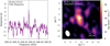 |
Fig. A.1 Left: filter response for a Keplerian mask, the HC3N J = 23−22 transition is marked with a dashed line. Right: Keplerian masked integrated intensity map. The beam is shown in the bottom left corner. |
Appendix B Modeling robustness
The effect of the C/O ratio, C/H abundance and the gas mass on the model is discussed in detail in Sect. 5. In this section the effect of other parameters such as the N/H abundance, ζ, fℓ and the extra dust in the cavity is investigated.
Appendix B.1 Parameter dependence
The results for a grid with varying specific model parameters are presented in Fig. B.1. We vary the nitrogen abundance between 10−4 − 10−7, ζ between 10−16 − 10−19 s−1 and fℓ between 0.99 and 0.5. Variations in the nitrogen abundance have no effect on the CO lines as these abundances are constrained by the availability of oxygen for C/O = 1. CN depends moderately on the nitrogen abundance, changing only a factor of two over 4 orders of magnitude difference in C/N. This means that CN is not a dominant carrier of N but that its abundance is set by other quantities such as the UV flux. The N2H+ emission is very sensitive to the nitrogen abundance, as the CO/N2 ratio has to be low to form N2H+ efficiently (see the discussion in Sect. 5.1.3). Unfortunately, we do not have the tools to determine the N/H abundance separately, considering CN is not sensitive to the N/H abundance. Nitrogen is thought to be less depleted than carbon (Bergin et al. 2015; Cleeves et al. 2018; Visser et al. 2018), given that the level of carbon depletion is low in this system the assumption of ISM level N/H is valid, but requires additional attention in the future.
Changing ζ has only effect on the optically thin CO lines as the rare CO isotopologues are less efficient in self-shielding against destruction. The ionization balance in the disk is mainly set by ζ, which results in a moderate dependence of N2H+ on ζ as discussed in Sect. 6.3.
Lowering fℓ will impact the vertical temperature structure as more surface area per dust mass unit is moved to the upper layers of the disk. High values for the large grain fractions are motivated by studies that find that mm-size dust can form on timescales of 105 yr (Ubach et al. 2012; Birnstiel et al. 2016). Lower values of fℓ are one of the only options to decrease the CN and 12CO flux and would increase the mass upper limit of the HD emission as it decreases the size of the HD emitting region. However, the effect on CN and 12CO is small and physical values <fℓ = 0.9 result in underproducing the CO isotopologue emission even taking higher C/H abundances and gas masses into account.
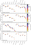 |
Fig. B.1 Total flux dependencies of the various molecules on the main parameters in the model. From top to bottom: Nitrogen abundance, cosmic ray ionization rate ζ, fraction of settled large grains fℓ. Data grid points and the fiducial model are shown in the colorbar as grey and white tickmarks, respectively. The color bars represent interpolated values between these models. The fiducial model is shown in the plots as a white dot. The bottom panel shows the result for a similar model as the fiducial model, but with a cleared cavity between 1-63 AU (see Fig. 3). Note that the fiducial model is the same as the “best” model in Fig. 2. |
Appendix B.2 Dust component in cavity
Motivated by the millimeter dust continuum observations presented in Facchini et al. (2020) we included a small contribution of dust inside the cavity to improve the fit on the millimeter continuum radial profile (see Fig. 3). This third dust ring could be a result of diffusing small grains inside the cavity or a planet. In the bottom panel of Fig. B.1 we compare the model fluxes with a model that uses the conventional transition disk setup with a cleared cavity and a small 1 AU inner disk (following the dashed line in Fig. 3). The dust surface density in the cavity in our fiducial model does not have a significant effect on the disk integrated line fluxes.
References
- Anderson, D. E., Blake, G. A., Bergin, E. A., et al. 2019, ApJ, 881, 127 [Google Scholar]
- Anderson, D. E., Cleeves, L. I., Blake, G. A., et al. 2022, ApJ, 927, 229 [NASA ADS] [CrossRef] [Google Scholar]
- Andrews, S. M., Wilner, D. J., Espaillat, C., et al. 2011, ApJ, 732, 42 [Google Scholar]
- Andrews, S. M., Rosenfeld, K. A., Kraus, A. L., & Wilner, D. J. 2013, ApJ, 771, 129 [Google Scholar]
- Andrews, S. M., Terrell, M., Tripathi, A., et al. 2018, ApJ, 865, 157 [Google Scholar]
- Ansdell, M., Williams, J. P., van der Marel, N., et al. 2016, ApJ, 828, 46 [Google Scholar]
- Ansdell, M., Williams, J. P., Trapman, L., et al. 2018, ApJ, 859, 21 [NASA ADS] [CrossRef] [Google Scholar]
- Bai, X.-N., & Stone, J. M. 2010, ApJ, 722, L220 [Google Scholar]
- Bergin, E. A., Hogerheijde, M. R., Brinch, C., et al. 2010, A&A, 521, A33 [Google Scholar]
- Bergin, E. A., Cleeves, L. I., Gorti, U., et al. 2013, Nature, 493, 644 [Google Scholar]
- Bergin, E. A., Blake, G. A., Ciesla, F., Hirschmann, M. M., & Li, J. 2015, Proc. Natl. Acad. Sci. U.S.A., 112, 8965 [NASA ADS] [CrossRef] [Google Scholar]
- Bergin, E. A., Du, F., Cleeves, L. I., et al. 2016, ApJ, 831, 101 [Google Scholar]
- Bergner, J. B., Öberg, K. I., Bergin, E. A., et al. 2019, ApJ, 876, 25 [Google Scholar]
- Bergner, J. B., Öberg, K. I., Bergin, E. A., et al. 2020, ApJ, 898, 97 [NASA ADS] [CrossRef] [Google Scholar]
- Birnstiel, T., Fang, M., & Johansen, A. 2016, Space Sci. Rev., 205, 41 [Google Scholar]
- Bisschop, S. E., Fraser, H. J., Öberg, K. I., van Dishoeck, E. F., & Schlemmer, S. 2006, A&A, 449, 1297 [NASA ADS] [CrossRef] [EDP Sciences] [Google Scholar]
- Booth, R. A., Clarke, C. J., Madhusudhan, N., & Ilee, J. D. 2017, MNRAS, 469, 3994 [Google Scholar]
- Booth, A. S., Walsh, C., Ilee, J. D., et al. 2019, ApJ, 882, L31 [Google Scholar]
- Bosman, A. D., Bruderer, S., & van Dishoeck, E. F. 2017, A&A, 601, A36 [NASA ADS] [CrossRef] [EDP Sciences] [Google Scholar]
- Bosman, A. D., Walsh, C., & van Dishoeck, E. F. 2018, A&A, 618, A182 [NASA ADS] [CrossRef] [EDP Sciences] [Google Scholar]
- Bosman, A. D., Alarcón, F., Bergin, E. A., et al. 2021a, ApJS, 257, 7 [NASA ADS] [CrossRef] [Google Scholar]
- Bosman, A. D., Alarcón, F., Zhang, K., & Bergin, E. A. 2021b, ApJ, 910, 3 [NASA ADS] [CrossRef] [Google Scholar]
- Bosman, A. D., Bergin, E. A., Loomis, R. A., et al. 2021c, ApJS, 257, 15 [NASA ADS] [CrossRef] [Google Scholar]
- Bruderer, S. 2013, A&A, 559, A46 [NASA ADS] [CrossRef] [EDP Sciences] [Google Scholar]
- Bruderer, S., van Dishoeck, E. F., Doty, S. D., & Herczeg, G. J. 2012, A&A, 541, A91 [NASA ADS] [CrossRef] [EDP Sciences] [Google Scholar]
- Cardelli, J. A., Clayton, G. C., & Mathis, J. S. 1989, ApJ, 345, 245 [Google Scholar]
- Cardelli, J. A., Meyer, D. M., Jura, M., & Savage, B. D. 1996, ApJ, 467, 334 [Google Scholar]
- Cazzoletti, P., van Dishoeck, E. F., Visser, R., Facchini, S., & Bruderer, S. 2018, A&A, 609, A93 [NASA ADS] [CrossRef] [EDP Sciences] [Google Scholar]
- Chapillon, E., Guilloteau, S., Dutrey, A., & Piétu, V. 2008, A&A, 488, 565 [NASA ADS] [CrossRef] [EDP Sciences] [Google Scholar]
- Cleeves, L. I., Bergin, E. A., Öberg, K. I., et al. 2017, ApJ, 843, L3 [Google Scholar]
- Cleeves, L. I., Öberg, K. I., Wilner, D. J., et al. 2018, ApJ, 865, 155 [Google Scholar]
- Currie, T., Marois, C., Cieza, L., et al. 2019, ApJ, 877, L3 [Google Scholar]
- D’Alessio, P., Calvet, N., Hartmann, L., Franco-Hernández, R., & Servín, H. 2006, ApJ, 638, 314 [Google Scholar]
- Du, F., Bergin, E. A., Hogerheijde, M., et al. 2017, ApJ, 842, 98 [Google Scholar]
- Dutrey, A., Guilloteau, S., & Simon, M. 2003, A&A, 402, 1003 [NASA ADS] [CrossRef] [EDP Sciences] [Google Scholar]
- Eistrup, C., Walsh, C., & van Dishoeck, E. F. 2016, A&A, 595, A83 [NASA ADS] [CrossRef] [EDP Sciences] [Google Scholar]
- Endres, C. P., Schlemmer, S., Schilke, P., Stutzki, J., & Müller, H. S. P. 2016, J. Mol. Spectrosc., 327, 95 [NASA ADS] [CrossRef] [Google Scholar]
- Espaillat, C., D'Alessio, P., Hernández, J., et al. 2010, ApJ, 717, 441 [NASA ADS] [CrossRef] [Google Scholar]
- Facchini, S., Benisty, M., Bae, J., et al. 2020, A&A, 639, A121 [EDP Sciences] [Google Scholar]
- Favre, C., Cleeves, L. I., Bergin, E. A., Qi, C., & Blake, G. A. 2013, ApJ, 776, L38 [Google Scholar]
- Gaia Collaboration (Prusti, T., et al.) 2016, A&A, 595, A1 [NASA ADS] [CrossRef] [EDP Sciences] [Google Scholar]
- Gaia Collaboration (Brown, A. G. A., et al.) 2021, A&A, 649, A1 [NASA ADS] [CrossRef] [EDP Sciences] [Google Scholar]
- Geers, V. C., Augereau, J. C., Pontoppidan, K. M., et al. 2006, A&A, 459, 545 [NASA ADS] [CrossRef] [EDP Sciences] [Google Scholar]
- Hildebrand, R. H. 1983, QJRAS, 24, 267 [NASA ADS] [Google Scholar]
- Hogerheijde, M. R., Bergin, E. A., Brinch, C., et al. 2011, Science, 334, 338 [Google Scholar]
- Ilee, J. D., Walsh, C., Booth, A. S., et al. 2021, ApJS, 257, 9 [NASA ADS] [CrossRef] [Google Scholar]
- Isella, A., Pérez, L. M., & Carpenter, J. M. 2012, ApJ, 747, 136 [NASA ADS] [CrossRef] [Google Scholar]
- Jin, S., Isella, A., Huang, P., et al. 2019, ApJ, 881, 108 [NASA ADS] [CrossRef] [Google Scholar]
- Kama, M., Bruderer, S., Carney, M., et al. 2016a, VizieR Online Data Catalog: J/A+A/588/A108 [Google Scholar]
- Kama, M., Bruderer, S., van Dishoeck, E. F., et al. 2016b, A&A, 592, A83 [NASA ADS] [CrossRef] [EDP Sciences] [Google Scholar]
- Kama, M., Trapman, L., Fedele, D., et al. 2020, A&A, 634, A88 [NASA ADS] [CrossRef] [EDP Sciences] [Google Scholar]
- Kraus, A. L., & Ireland, M. J. 2012, ApJ, 745, 5 [Google Scholar]
- Krijt, S., Schwarz, K. R., Bergin, E. A., & Ciesla, F. J. 2018, ApJ, 864, 78 [Google Scholar]
- Krijt, S., Bosman, A. D., Zhang, K., et al. 2020, ApJ, 899, 134 [NASA ADS] [CrossRef] [Google Scholar]
- Le Gal, R., Brady, M. T., Öberg, K. I., Roueff, E., & Le Petit, F. 2019, ApJ, 886, 86 [NASA ADS] [CrossRef] [Google Scholar]
- Leemker, M., Booth, A. S., van Dishoeck, E. F., et al. 2022, A&A, 663, A23 [NASA ADS] [CrossRef] [EDP Sciences] [Google Scholar]
- Lissauer, J. J., & Stevenson, D. J. 2007, in Protostars and Planets V, 591 [Google Scholar]
- Lodders, K. 2010, Exoplanet Chemistry (Wiley), 157 [Google Scholar]
- Long, F., Herczeg, G. J., Pascucci, I., et al. 2017, ApJ, 844, 99 [Google Scholar]
- Loomis, R. A., Öberg, K. I., Andrews, S. M., et al. 2018, AJ, 155, 182 [Google Scholar]
- Loomis, R. A., Öberg, K. I., Andrews, S. M., et al. 2020, ApJ, 893, 101 [Google Scholar]
- Madhusudhan, N. 2019, ARA&A, 57, 617 [NASA ADS] [CrossRef] [Google Scholar]
- McClure, M. K., Bergin, E. A., Cleeves, L. I., et al. 2016, ApJ, 831, 167 [Google Scholar]
- McMullin, J. P., Waters, B., Schiebel, D., Young, W., & Golap, K. 2007, ASP Conf. Ser. 376, 127 [Google Scholar]
- Meyer, D. M., Jura, M., & Cardelli, J. A. 1998, ApJ, 493, 222 [CrossRef] [Google Scholar]
- Miotello, A., Bruderer, S., & van Dishoeck, E. F. 2014, A&A, 572, A96 [NASA ADS] [CrossRef] [EDP Sciences] [Google Scholar]
- Miotello, A., van Dishoeck, E. F., Kama, M., & Bruderer, S. 2016, A&A, 594, A85 [NASA ADS] [CrossRef] [EDP Sciences] [Google Scholar]
- Miotello, A., van Dishoeck, E. F., Williams, J. P., et al. 2017, A&A, 599, A113 [NASA ADS] [CrossRef] [EDP Sciences] [Google Scholar]
- Miotello, A., Facchini, S., van Dishoeck, E. F., et al. 2019, A&A, 631, A69 [NASA ADS] [CrossRef] [EDP Sciences] [Google Scholar]
- Mordasini, C., Alibert, Y., Benz, W., Klahr, H., & Henning, T. 2012, A&A, 541, A97 [NASA ADS] [CrossRef] [EDP Sciences] [Google Scholar]
- Öberg, K. I., Qi, C., Fogel, J. K. J., et al. 2010, ApJ, 720, 480 [Google Scholar]
- Öberg, K. I., Murray-Clay, R., & Bergin, E. A. 2011a, ApJ, 743, L16 [Google Scholar]
- Öberg, K. I., Qi, C., Fogel, J. K. J., et al. 2011b, ApJ, 734, 98 [Google Scholar]
- Oh, D., Hashimoto, J., Tamura, M., et al. 2016, PASJ, 68, L3 [Google Scholar]
- Parvathi, V. S., Sofia, U. J., Murthy, J., & Babu, B. R. S. 2012, ApJ, 760, 36 [NASA ADS] [CrossRef] [Google Scholar]
- Pegues, J., Öberg, K. I., Bergner, J. B., et al. 2020, ApJ, 890, 142 [Google Scholar]
- Piétu, V., Dutrey, A., Guilloteau, S., Chapillon, E., & Pety, J. 2006, A&A, 460, L43 [NASA ADS] [CrossRef] [EDP Sciences] [Google Scholar]
- Pinilla, P., Benisty, M., & Birnstiel, T. 2012, A&A, 545, A81 [NASA ADS] [CrossRef] [EDP Sciences] [Google Scholar]
- Pirovano, L. M., Fedele, D., van Dishoeck, E. F., et al. 2022, A&A, 665, A45 [NASA ADS] [CrossRef] [EDP Sciences] [Google Scholar]
- Qi, C., Öberg, K. I., Espaillat, C. C., et al. 2019, ApJ, 882, 160 [Google Scholar]
- Sallum, S., Follette, K. B., Eisner, J. A., et al. 2015, Nature, 527, 342 [Google Scholar]
- Salyk, C., Blake, G. A., Boogert, A. C. A., & Brown, J. M. 2009, ApJ, 699, 330 [NASA ADS] [CrossRef] [Google Scholar]
- Schwarz, K. R., Bergin, E. A., Cleeves, L. I., et al. 2018, ApJ, 856, 85 [Google Scholar]
- Sturm, J. A., McClure, M. K., Harsono, D., et al. 2022, A&A, 660, A126 [NASA ADS] [CrossRef] [EDP Sciences] [Google Scholar]
- Tafalla, M., & Santiago, J. 2004, A&A, 414, L53 [NASA ADS] [CrossRef] [EDP Sciences] [Google Scholar]
- Thalmann, C., Janson, M., Garufi, A., et al. 2016, ApJ, 828, L17 [Google Scholar]
- Trapman, L., Miotello, A., Kama, M., van Dishoeck, E. F., & Bruderer, S. 2017, A&A, 605, A69 [NASA ADS] [CrossRef] [EDP Sciences] [Google Scholar]
- Trapman, L., Zhang, K., van't Hoff, M. L. R., Hogerheijde, M. R., & Bergin, E. A. 2022, ApJ, 926, L2 [NASA ADS] [CrossRef] [Google Scholar]
- Ubach, C., Maddison, S. T., Wright, C. M., et al. 2012, MNRAS, 425, 3137 [NASA ADS] [CrossRef] [Google Scholar]
- van der Marel, N., van Dishoeck, E. F., Bruderer, S., Pérez, L., & Isella, A. 2015, A&A, 579, A106 [NASA ADS] [CrossRef] [EDP Sciences] [Google Scholar]
- van der Marel, N., Bosman, A. D., Krijt, S., Mulders, G. D., & Bergner, J. B. 2021, A&A, 653, A9 [NASA ADS] [CrossRef] [EDP Sciences] [Google Scholar]
- van Dishoeck, E. F., Kristensen, L. E., Mottram, J. C., et al. 2021, A&A, 648, A24 [NASA ADS] [CrossRef] [EDP Sciences] [Google Scholar]
- van’t Hoff, M. L. R., Walsh, C., Kama, M., Facchini, S., & van Dishoeck, E. F. 2017, A&A, 599, A101 [Google Scholar]
- van Zadelhoff, G. J., van Dishoeck, E. F., Thi, W. F., & Blake, G. A. 2001, A&A, 377, 566 [NASA ADS] [CrossRef] [EDP Sciences] [Google Scholar]
- Visser, R., Bruderer, S., Cazzoletti, P., et al. 2018, A&A, 615, A75 [NASA ADS] [CrossRef] [EDP Sciences] [Google Scholar]
- Weingartner, J. C., & Draine, B. T. 2001, ApJ, 548, 296 [Google Scholar]
- Williams, J. P., & Best, W. M. J. 2014, ApJ, 788, 59 [Google Scholar]
- Wilson, T. L. 1999, Rep. Progr. Phys., 62, 143 [CrossRef] [Google Scholar]
- Zhang, K., Bergin, E. A., Schwarz, K., Krijt, S., & Ciesla, F. 2019, ApJ, 883, 98 [Google Scholar]
- Zhang, K., Bosman, A. D., & Bergin, E. A. 2020a, ApJ, 891, L16 [NASA ADS] [CrossRef] [Google Scholar]
- Zhang, K., Schwarz, K. R., & Bergin, E. A. 2020b, ApJ, 891, L17 [Google Scholar]
All Tables
All Figures
|
Fig. 1 Disk-integrated spectra (top) and total intensity or moment 0 maps of the new emission lines (bottom) obtained with NOEMA at 1.1″ × 0.7″. ALMA band 6 continuum data at 0.3″ × 0.3″ are shown for comparison. Integration limits for the moment 0 maps are indicated with black tickmarks in the bottom at −4 and +4 km s−1. Robustly detected CN hyper-fine structure lines are indicated in the top right panel with black tick marks. For each moment 0 map, the beam is shown as a white ellipse in the lower left corner. |
| In the text | |
|
Fig. 2 Azimuthally averaged radial proflies of the different gas tracers used in this work (left). Data are shown as black lines with shaded 1 σ uncertainty and normalized to the brightest point for visualization purposes. The full width at half maximum of the beams is shown as a black horizontal line in the lower left-hand corner. The best-fitting model with a gas mass of 0.012 M⊙ and a factor of 4 in carbon depletion is overplotted in red. The blue line shows the same model but with a lower gas-to-dust ratio, resulting in a gas mass of 4 × 10⁻⁴ M⊙, and no carbon depletion. This model reproduces the optically thick CN and CO lines somewhat better, but underproduces the optically thin N2H+ line. The orange line illustrates the C2H radial profile for an increased C/O ratio of 1.1. With C/O > 1 excess carbon, not in CO, changes the carbon chemistry completely. Integrated line flux of the various emission lines analyzed in this paper (right). Black squares represent the observed line fluxes of NOEMA data, black diamonds represent the observed line fluxes of ALMA data, black triangles denote upper limits, taken at 3σ. Colored diamonds show the results for the same models as in the left panel. |
| In the text | |
|
Fig. 3 Setup of the DALI model for LkCa 15, top-left: normalized surface density of the dust (orange) and gas (blue) as function of radius, bottom-left: gas-to-dust ratio as function of radius in the fiducial model, this is a direct consequence of the used gas and dust surface density profiles shown in the top left panel, top-right: radial profile of the continuum observations (black) and the model (orange) normalized to 1, bottom-right: observed SED in black with the modeled continuum fluxes in orange. Dashed lines show the setup for the same model with cleared cavity, discussed in Appendix B. |
| In the text | |
|
Fig. 4 Emitting heights of the 12CO (orange) and 13CO (blue) J = 2−1 emission, taken from Leemker et al. (2022). Scattered points represent the emitting height for each channel, whereas the solid line represents a radially binned average with 1er error. The dashed line shows the height of the τ = 1 line in the DALI model. The disk is flat in both the observations as well as the model. |
| In the text | |
|
Fig. 5 Overview of the DALI model output. The four panels left top (A−D) present the gas and dust density structure and the gas and dust temperature, respectively. The other panels present the molecular abundances of the molecular transitions in the most representative DALI model, assuming a gas-to-dust ratio of 25 and a carbon depletion factor of 4. The white contours represent the region where 95% of the emission originates, the black lines show the τ = 1 surface for the optically thick emission lines. |
| In the text | |
|
Fig. 6 Results of the 10 × 6 model grid with carbon abundance versus disk gas mass. Panel A shows the limits on C/H and Mgas for each emission line, assuming a model uncertainty of a factor of 2. The hashed region denotes the parameter space that matches with all the observed emission lines. Panels B–F show the line flux of key C/H abundance and gas mass tracers N2H+, CN, C17O, HD, and 12CO, respectively, for the same grid of models. The white contours depict the observed flux with observational uncertainty in shaded region. The colored contours mark an average deviation of the model by a factor of 2, the same as in the main panel. The HD observation denotes an upper limit. |
| In the text | |
|
Fig. A.1 Left: filter response for a Keplerian mask, the HC3N J = 23−22 transition is marked with a dashed line. Right: Keplerian masked integrated intensity map. The beam is shown in the bottom left corner. |
| In the text | |
|
Fig. B.1 Total flux dependencies of the various molecules on the main parameters in the model. From top to bottom: Nitrogen abundance, cosmic ray ionization rate ζ, fraction of settled large grains fℓ. Data grid points and the fiducial model are shown in the colorbar as grey and white tickmarks, respectively. The color bars represent interpolated values between these models. The fiducial model is shown in the plots as a white dot. The bottom panel shows the result for a similar model as the fiducial model, but with a cleared cavity between 1-63 AU (see Fig. 3). Note that the fiducial model is the same as the “best” model in Fig. 2. |
| In the text | |
Current usage metrics show cumulative count of Article Views (full-text article views including HTML views, PDF and ePub downloads, according to the available data) and Abstracts Views on Vision4Press platform.
Data correspond to usage on the plateform after 2015. The current usage metrics is available 48-96 hours after online publication and is updated daily on week days.
Initial download of the metrics may take a while.