| Issue |
A&A
Volume 669, January 2023
|
|
|---|---|---|
| Article Number | A90 | |
| Number of page(s) | 21 | |
| Section | Interstellar and circumstellar matter | |
| DOI | https://doi.org/10.1051/0004-6361/202243813 | |
| Published online | 16 January 2023 | |
Magnetically regulated collapse in the B335 protostar?
II. Observational constraints on gas ionization and magnetic field coupling
1
Université Paris-Saclay, Université Paris Cité, CEA, CNRS, AIM,
91191
Gif-sur-Yvette, France
2
Institut de Ciències de l’Espai (ICE), CSIC,
Can Magrans s/n,
E-08193
Cerdanyola del Vallès, Catalonia, Spain
3
Institute of Chemical Sciences, School of Engineering and Physical Sciences, Heriot-Watt University,
EH14 4AS,
Edinburgh, Scotland
e-mail: This email address is being protected from spambots. You need JavaScript enabled to view it.
4
Center for Astrophysics | Harvard & Smithsonian,
60 Garden Street,
Cambridge, MA
02138, USA
5
Institut d’Estudis Espacials de Catalunya (IEEC),
E-08034
Barcelona, Catalonia, Spain
6
INAF–Osservatorio Astrofisico di Arcetri,
Largo E. Fermi 5,
50125
Firenze, Italy
7
Department of Physics and Astronomy, The University of Western Ontario,
1151 Richmond Street,
London, Ontario
N6A 3K7, Canada
Received:
19
April
2022
Accepted:
20
September
2022
Abstract
Context. Whether or not magnetic fields play a key role in dynamically shaping the products of the star formation process is still largely debated. For example, in magnetized protostellar formation models, magnetic braking plays a major role in the regulation of the angular momentum transported from large envelope scales to the inner envelope, and is expected to be responsible for the resulting protostellar disk sizes. However, non-ideal magnetohydrodynamic effects that rule the coupling of the magnetic field to the gas also depend heavily on the local physical conditions, such as the ionization fraction of the gas.
Aims. The purpose of this work is to observationally characterize the level of ionization of the gas at small envelope radii and to investigate its relation to the efficiency of the coupling between the star-forming gas and the magnetic field in the Class 0 protostar B335.
Methods. We obtained molecular line emission maps of B335 with ALMA, which we use to measure the deuteration fraction of the gas, RD, its ionization fraction, χe, and the cosmic-ray ionization rate, ζCR, at envelope radii ≲1000 au.
Results. We find large fractions of ionized gas, χe ≃ 1–8 × 10⁻⁶. Our observations also reveal an enhanced ionization that increases at small envelope radii, reaching values up to ζCR ≃ 10−14 s−1 at a few hundred astronomical units (au) from the central protostellar object. We show that this extreme ζCR can be attributed to the presence of cosmic rays accelerated close to the protostar.
Conclusions. We report the first resolved map of ζCR at scales ≲1000 au in a solar-type Class 0 protostar, finding remarkably high values. Our observations suggest that local acceleration of cosmic rays, and not the penetration of interstellar Galactic cosmic rays, may be responsible for the gas ionization in the inner envelope, potentially down to disk-forming scales. If confirmed, our findings imply that protostellar disk properties may also be determined by local processes that set the coupling between the gas and the magnetic field, and not only by the amount of angular momentum available at large envelope scales and the magnetic field strength in protostellar cores. We stress that the gas ionization we find in B335 significantly stands out from the typical values routinely used in state-of-the-art models of protostellar formation and evolution. If the local processes of ionization uncovered in B335 are prototypical to low-mass protostars, our results call for a revision of the treatment of ionizing processes in magnetized models for star and disk formation.
Key words: stars: formation / circumstellar matter / magnetic fields / techniques: interferometric
© The Authors 2023
 Open Access article, published by EDP Sciences, under the terms of the Creative Commons Attribution License (https://creativecommons.org/licenses/by/4.0), which permits unrestricted use, distribution, and reproduction in any medium, provided the original work is properly cited.
This article is published in open access under the Subscribe-to-Open model. This email address is being protected from spambots. You need JavaScript enabled to view it. to support open access publication.
1 Introduction
Observational studies have shown that magnetic fields are present at all scales where star formation processes are at work, permeating molecular clouds, prestellar cores, and protostellar envelopes (e.g., Girart et al. 2006; Alves et al. 2014; Zhang et al. 2014; Soler 2019). While magnetized models of star formation were developed early on, it is only recently that complex physics has been included in numerical magnetohydrodynamic (MHD) models, and that the predictions of dedicated models are directly compared to observations of star-forming regions. One of the major achievements of magnetized models is the prediction of the small sizes of protostellar disks, regulated by magnetic braking (Dapp et al. 2012; Hennebelle & Inutsuka 2019; Zhao et al. 2020). Recent observations have indeed shown that disks are compact, and are almost an order of magnitude smaller than those produced in purely hydrodynamical models (Maury et al. 2019; Lebreuilly et al. 2021).
In magnetized collapse models, non-ideal MHD effects play a major role in the regulation of magnetic flux during the early stages of protostellar formation (Machida et al. 2011; Li et al. 2011; Marchand et al. 2020). Hence, these processes indirectly limit the angular momentum transported by the magnetic field from large envelope scales to the inner envelope, and set the resulting disk size. However, these resistive processes depend heavily on the local physical conditions, such as dust grain properties (electric charge and size), gas density and temperature, density of ions and electrons, and the cosmic-ray (CR) ionization rate, ζCR (namely the number of molecular hydrogen ionizations per unit time; see e.g., Zhao et al. 2020, for a review). Observationally, only very few measurements of these quantities have been obtained toward solar-type protostars: the effective coupling of magnetic fields to the infalling-rotating material, at scales where the circumstellar material feeds the growth in mass of the protostellar embryo and its disk, is therefore still largely unknown.
B335, located at a distance of 164.5 pc (Watson 2020), is an isolated Bok Globule which contains an embedded Class 0 protostar (Keene et al. 1983). The core is associated with an east-west outflow that is prominently detected in CO, with an inclination of 10° on the plane of the sky and an opening angle of 45° (Hirano et al. 1988, Hirano et al. 1992; Stutz et al. 2008; Yen et al. 2010). Its isolation and relative proximity makes B335 an ideal object with which to test models of star formation. Asymmetric double-peaked line profiles observed in the molecular emission of the gas toward the envelope have been interpreted as optically thick lines tracing infalling motions, and have been extensively used to derive mass-infall rates from 10−7 to ~3 × 10⁻⁶ M⊙ yr−1 at radii of 100-2000 au (Zhou et al. 1993; Yen et al. 2010; Evans et al. 2015). However, new observations of optically thin emission from less abundant molecules reveal the presence of two velocity components tracing asymmetric motions at these envelope scales, which could contribute significantly to the double-peaked line profiles (Cabedo et al. 2021). These results suggest that simple spherically symmetric infall models might not be adequate to describe the collapse of the B335 envelope, and tentatively unveil the existence of preferential accretion streamlines along outflow cavity walls.
B335 is also an excellent prototype for the study of magnetized star-formation models, because it has been proposed as an example of a protostar where the disk size is set by a magnetically regulated collapse (Maury et al. 2018, hereafter Paper I). This hypothesis rests mainly on two observations. First, the rotation of the gas observed at large envelope radii is not found at small envelope radii (<1000 au) and no kinematic signature of a disk was reported down to ~ 10 au (Kurono et al. 2013; Yen et al. 2015). Second, observations of polarized dust emission have revealed an “hourglass” magnetic field morphology (Paper I) in the inner envelope: comparisons to MHD models of protostellar formation (see e.g., Masson et al. 2016; Hennebelle et al. 2020, for a whole description of the models) suggest that the B335 envelope is threaded by a rather strong magnetic field which is highly coupled to the infalling-rotating gas, preventing disk growth out to large radii. The purpose of the analysis presented here is to characterize the level of ionization and its origin in order to test the model scenario proposed in Paper I, and put observational constraints on the efficiency of the coupling of the magnetic field to the star-forming gas in the inner envelope of B335.
In Sect. 2, we present the ALMA observations used to constrain physical and chemical properties of the gas at envelope radii ≲1000 au. In Sect. 3, we derive the deuteration fraction, Rd, from DCO+ (J = 3–2) and H13CO+ (J = 3–2). In Sect. 4, we compute the ionization fraction, χe, and the ζCR. Finally, in Sect. 5, we discuss our results concerning deuteration processes, the ionization, the possible influence of a local source of radiation and its effect on the coupling between the gas and the magnetic field.
2 Observations and data reduction
Observations of the Class 0 protostellar object B335 were carried out with the ALMA interferometer during the Cycle 4 observation period, from October 2016 to September 2017, as part of the 2016.1.01552.S project. The centroid position of B335 is assumed to be α = 19 : 37 : 00.9 and δ = +07 : 34 : 09.6 (in J2000 coordinates) based on the dust continuum peak obtained by Maury et al. (2018).
We used DCO+ (J = 3–2) and H13CO+ (J = 3–2) to obtain RD and χe. We used H13CO+ (J = 1–0) and C17O (J = 1–0) to derive the hydrogenation fraction, RH. Additionally, we observed the dust continuum at 110 GHz to derive the estimated line opacities, CO depletion factor, fD, and ζCR. We also targeted 12CO (J = 2–1) and N2D+ (J = 3–2) for comparison purposes. All lines were targeted using a combination of ALMA configurations to recover the largest length-scale range possible. As our data for H13CO+ (J = 3–2) only include observations with the Atacama Compact Array (ACA), we used additional observations of this molecular line at smaller scales from the ALMA project 2015.1.01188.S. Technical details of the ALMA observations are shown in Appendix A.
Calibration of the raw data was done using the standard script for Cycle 4 ALMA data and the Common Astronomy Software Applications (CASA), version 5.6.1–8. The continuum emission was self-calibrated with CASA. Line emission from 12CO (J = 2–1) and N2D+ (J = 3–2) was additionally calibrated using the self-calibrated continuum model at the appropriate frequency (231 GHz, not shown in this work).
Final images of the data were generated from the calibrated visibilities using the tCLEAN algorithm within CASA, using Briggs weighting with a robust parameter of 1 for all the tracers. As we want to compare our data to the C17O (J = 1–0) emission presented in Cabedo et al. (2021), we adjust our imaging parameters to obtain matching beam maps with similar angular and spectral resolution. For DCO+ (J = 3–2) and H13CO+ (J = 3–2), we restricted the baselines to a common “u, v” range between 9 and 140 kλ, and finally smoothed them to the same angular resolution. The preliminary analysis shows that both C17O (J = 1–0) and H13CO+ (J = 1–0) emission is barely detected in the most extended configurations. We proceed by applying a common “uv tapering” of 1.5″ to both lines. This procedure allows to decrease the weighting of the largest baselines in our analysis, giving more weight to the smaller baselines and allowing us to obtain a better signal-to-noise ratio (S/N). Furthermore, we smoothed the data to obtain exactly the same angular resolution. Additionally, we smooth C17O (J = 1–0) and the dust continuum at 110 GHz to obtain DCO+ matching beam maps to compute fD. The imaging parameters used to obtain all the spectral cubes and their final characteristics are shown in Table 1. Even though the characteristics and properties of the C17O (J = 1–0) maps are slightly different from the ones presented in Cabedo et al. (2021) due to the differences in the imaging process, the line profiles show the same characteristics (i.e., line profiles are double-peaked and present the same velocity pattern at different offsets from the center of the source) confirming that the imaging process has no large effect on the shape of the line profile, and that the two velocity components can still be observed.
Data products
From the data cubes, we obtained spectral maps that present the spectrum (in velocity units) at each pixel of a determined region around the center of the source. These maps allow us to evaluate the spectra at different offsets from the center of the envelope where the dust continuum emission peak localizes the protostar, and to detect any distinct line profile or velocity pattern. The obtained spectral maps are discussed in Appendix B.1.
We derived the integrated intensity maps by integrating the molecular line emission over the velocity range in which it is emitting (the velocity range used for each molecule is shown in Table 1). Figure 1 shows the dust continuum emission map at 110 GHz and the integrated intensity contours of C17O (J = 1–0), DCO+ (J = 3–2), H13CO+ (J = 1–0), and H13CO+ (J = 3–2). The H13CO+ (J = 1–0) emission clearly appears more spatially extended than the other lines, roughly following most of the dust emission. The emission from this line extends further than the dust toward the southeast outflow cavity wall direction. The C17O (J = 1–0), DCO+ (J = 3–2), and H13CO+ (J = 3–2) emission present a similar, relatively compact morphology centered around the dust peak and elongated along the north-south equatorial plane. However, the spatial extent along the equatorial plane is slightly more compact for the H13CO+ emission (~2100 au) than the DCO+ emission (~2500 au), and both are more extended than C17O (~1700 au). The DCO+ peak intensity is clearly more displaced from the continuum peak than the H13CO+ (J = 3–2) peak; this could be a local effect around the protostar due to the large temperature and irradiation conditions, which destroy DCO+ (Wootten 1987; Butner et al. 1995). The C17O (J = 1–0) emission appears to be slightly extended along the outflow cavities.
As all the molecules present a double-peaked profile with similar velocity patterns to the ones observed in Cabedo et al. (2021), namely two different velocity components with varying intensity across the source spatial extent, we use two independent velocity components to fit the line profiles simultaneously. Following Cabedo et al. (2021), we modeled the spectrum at each pixel using the HfS fitting program (Estalella 2017). We obtained maps of peak velocity and velocity dispersion for each velocity component, deriving the corresponding uncertainties from the χ2 goodness of fit (see Estalella 2017, for a thorough description of the derivation of uncertainties). A more detailed discussion of these maps is presented in Appendix B.2. In addition, an estimate of line opacities is given in Appendix C. In the following sections, the statistical uncertainties derived (shown in Figs. 2, 4, and 5) are computed using standard error propagation analysis from the uncertainties of each parameter obtained with the line modeling (peak velocity, velocity dispersion, and opacity). Other systematic uncertainties are discussed separately in the corresponding sections.
Imaging parameters and final map characteristics.
3 Deuteration fraction
The process of deuteration consists of an enrichment of the amount of deuterium with respect to hydrogen in molecular species. The deuteration fraction, RD,= [D]/[H], in molecular ions, in particular HCO+, has been extensively used as an estimator of the degree of ionization in molecular gas (Caselli et al. 1998; Fontani et al. 2017). Here, we apply this method to obtain maps of RD, computed as the column density ratio of DCO+ (J = 3–2) and its non-deuterated counterpart, H13CO+ (J = 3–2):
 (1)
(1)
where Ni is the column density of each species and  is the abundance ratio of 12C to 13C. The column density of both species is computed such as:
 (2)
(2)
where λ is the wavelength of the transition, A is the Einstein coefficient, Jv(T) is the Planck function at the background (2.7 K) and at the excitation temperature of the line (assumed to be equal to the dust temperature at the observed scales, Tex = Td = 25 K, Galametz et al. 2019; Cabedo et al. 2021), kB is the Boltzmann constant, gu is the upper state degeneracy, Qrot is the partition function at 25 K, El is the energy of the lower level, and ∫I0dv is the integrated intensity. Values of these parameters for each molecule are listed in Table 2.
The top panels of Fig. 2 show the RD maps of B335 for the blue- and redshifted velocity components (left and right column, respectively). The mean values of RD are ~ 1–2%, being higher in the outer region of the envelope where the gas is expected to be colder, and decreasing toward the center where the protostar is located and the temperature is expected to rise. The bottom panels show that the statistical uncertainties are roughly one-tenth of the deuteration values. We note that the highest values of RD are found for the blueshifted component, as high as 3.5%. However, these values have the largest associated errors due to the presence of a third velocity component in the line profiles of H13CO+ (J = 3–2) and should not be totally trusted (see Appendix B.1). Finally, we note that while the average RD values for both velocity components are similar, the most widespread blueshifted gas component shows larger RD dispersion, with values from 0.06% to 2%, while the more localized redshifted gas exhibits more uniform values, between 0.01% and 1%.
One of the main uncertainties of the deuteration analysis is the assumption that both DCO+ (J = 3–2) and H13CO+ (J = 3–2) have the same Tex. This should be accurate enough, because both molecules present a similar geometry and dipolar moment and are assumed to be spatially coexistent. However, to check the effect that the variation of Tex would produce in our values, we computed the column densities of both species at two additional temperatures, 20 and 30 K. While the DCO+ column density does not change significantly at these two temperatures with respect to the value adopted (25 K), the H13CO+ column density changes by about 15%. Nevertheless, the new values are still in agreement with the derived values of RD from DCO+ reported in the literature (see Sect. 5.1).
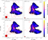 |
Fig. 1 Map of the dust continuum emission at 110 GHz clipped for values smaller than 3σ (see Table 1) and integrated emission for the four molecular lines as indicated in the upper left corner (red contours). Contours are −2, 3, 5, 8, 11, 14, and 17σ (the individual σ values are indicated in Table 1). The velocity ranges used to obtain the integrated intensity maps are shown in Table 1. In the bottom-left of each plot, we show the beam size for each molecular line (in red) and for the dust continuum emission (in black). The physical scale is shown in the top-right corner of the figure. |
Parameters for the computation of the column density.
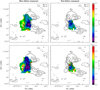 |
Fig. 2 Dust continuum emission at 110 GHz for −2, 3, 5, 7, 10, 30, and 50σ (black contours) superimposed on the deuteration fraction maps (top panels) and on the corresponding statistical uncertainties (lower panels) for the blue- and redshifted velocity components (left and right columns, respectively). The spatial scale is shown in the top-right corner of the upper panels. |
4 Ionization fraction and cosmic-ray ionization rate
We followed the method presented in Caselli et al. (1998) to compute χe and ζCR from RD. The two quantities are given by
 (3)
(3)
and
![Mathematical equation: ${\zeta _{{\rm{CR}}}} = \left[ {7.5 \times {{10}^{ - 4}}{\chi _{\rm{e}}} + {{4.6 \times {{10}^{ - 10}}} \over {{f_D}}}} \right]{\chi _{\rm{e}}}{n_{{{\rm{H}}_2}}}{R_{\rm{H}}},$](/articles/aa/full_html/2023/01/aa43813-22/aa43813-22-eq6.png) (4)
(4)
where fD is the depletion fraction of C and O,  is the H2 volume density, and RH is the hydrogenation fraction, Rh = [HCO+]/[CO].
While this observational method to measure χe of the gas relies on a simple chemical network and a rather strong hypothesis, it is widely used in the literature in dense cores and also toward protostars. The validity and shortcomings of the chemical models used to constrain ionization fractions are concisely discussed in Sect. 5.3.
4.1 Estimate of the CO depletion in B335
As RD, and therefore χe, depend on the level of C and O depletion from the gas phase, we hypothesize that the CO abundance is proportional to the CO column density and estimated fD as the ratio between the “expected”,  , and the “observed” CO column density,
  :
:
 (5)
(5)
Here,  is computed as the product of the H2 column density,
  , and the expected CO to H2 abundance ratio, XCO = [CO]/[H2] = 10−4 (Wilson & Rood 1994; Gerner et al. 2014), and NO is derived as the product of the C17O column density,
  , and the C17O to CO abundance ratio,
 ![Mathematical equation: ${f_{{{\rm{C}}^{17}}{\rm{O}}}} = \left[ {{\rm{CO}}} \right]/\left[ {{{\rm{C}}^{17}}{\rm{O}}} \right] = 2317$](/articles/aa/full_html/2023/01/aa43813-22/aa43813-22-eq14.png) (Wouterloot et al. 2008). Then, fD is given by
(Wouterloot et al. 2008). Then, fD is given by
 (6)
(6)
The H2 column density has been estimated from the dust thermal emission at 110 GHz (see Fig. 1) corrected for the primary beam attenuation. Indeed,  depends directly on the flux density measured on the continuum map, the beam solid angle Ωbeam, the Planck function Bν(Td) at the dust temperature, and the dust mass opacity κν (in units of cm2 g−1) at the frequency at which the dust thermal emission was observed:
![Mathematical equation: ${N_{{{\rm{H}}_2}}} = - {1 \over {{\mu _{{{\rm{H}}_2}}}{m_{\rm{H}}}{\kappa _v}}}\ln \left[ {1 - {{S_v^{{\rm{beam}}}} \over {{{\rm{\Omega }}_{{\rm{beam}}}}{B_v}\left( {{T_d}} \right)}}} \right],$](/articles/aa/full_html/2023/01/aa43813-22/aa43813-22-eq17.png) (7)
(7)
where  , mH is the atomic hydrogen mass, and for the dust opacity we used a power-law fit given by
 (8)
(8)
We adopt a dust mass absorption coefficient κ0 = 1.6 cm2 g−1 at λ0 = 1.3 mm, following Ossenkopf & Henning (1994). We assume a standard gas-to-dust ratio χd = 100, a dust emissivity exponent β = 0.76 (Galametz et al. 2019), and a dust temperature Td = 25 K. The resulting  column densities probed in the ALMA dust continuum emission map range from ~1020 cm−2 at radii of ~1600 au up to a few 1022 cm−2 at the protostar position. We note that the values of column density suffer from a systematic error due to assumptions on the parameters used to derive them (e.g., dust opacity, dust temperature). We estimate that the systematic error is about a factor of 3–5, being higher toward the peak position where standard dust properties and conditions of emission may not be met. We use Eq. (2) to estimate the observed CO column density
  from the C17O emission map shown in Fig. 1, assuming an excitation temperature of 25 K. The CO column density values are subject to systematic uncertainties due to the adopted gas temperature, as this latter is not well constrained and is expected to vary across the envelope. Altogether, the systematic uncertainty is about a factor of 2, and is higher toward the peak position where different gas temperatures are expected to be present along the line of sight.
Using Eq. (6), we obtain the CO depletion fraction map shown in Fig. 3. The depletion factor ranges from ~20 in the outer regions to ~70 in the center of the object. Propagating the errors from the column density maps they stem from, we expect these depletion values to have an uncertainty of a factor of 2–3, as the main source of errors – which are due to the assumed gas and dust temperatures – are lessened by the ratio. The CO depletion seems highly asymmetric around the protostar, being the lowest in the southeastern quadrant, while high values are associated to the protostar position and the northern region. We note that the regions with high fD coincide with the regions of low deuteration shown in Fig. 2.
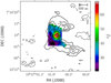 |
Fig. 3 Map of the CO depletion factor and contours of dust continuum emission at 110 GHz, for emission over 3σ. The spatial scale is shown in the top-right corner of the figure. |
4.2 Ionization fraction of the gas
We obtained χe using our RD maps, shown in Sect. 3 and the CO depletion map, presented in Fig. 3. The top panels of Fig. 4 show the derived χe and the bottom panels the associated uncertainties, for the blue- and red-shifted velocity components (left and right column, respectively). We obtained a mean value of χe = 2 × 10⁻⁶ for both components. Generally, these values are subject to statistical uncertainties of ~1.5 × 10⁻⁶. The range of values found for RD and fD indicates that the χe depends mostly on the level of deuteration, and therefore the systematic errors on the estimated χe from Eq. (3) are typically < 30% and statistical uncertainties dominate in this case. As RD decreases toward the center of the source, we find that χe increases toward the center.
4.3 Derivation of the CR ionization rate
We produced ζCR maps using Eq. (4). We obtained  as
as  , using the
  map obtained in Sect. 4.1 and considering a core diameter, L, of 1720 au derived from the C17O (J = 1–0) emission (Cabedo et al. 2021). With this approximation, we find values of the volume density ranging from ~104 in the outer regions, to ~106 cm−3 at the protostar position. We obtained Rh for both velocity components as the column density ratio of H13CO+ (J = 1–0) to C17O (J = 1–0), and accounting for
  and
and  :
:
 (9)
(9)
Values of RH are relatively uniform across the source, with mean values between 2 and 3 × 10⁻⁷ for the two velocity components. The statistical uncertainties of these values are generally one order of magnitude smaller than RH.
The two terms within the brackets in Eq. (4) have values of the order of ~10−9 and ~10−11, respectively. Therefore, the derivation of ζCR is very sensitive to χe but not to fD. The top panels of Fig. 5 show the derived ζCR and the bottom panels show the associated statistical uncertainties, for the blue- and redshifted velocity components (left and right column, respectively). As expected from the values of χe, ζCR increases toward the center, reaching values of 7 × 10⁻¹⁴ s−1 at the peak of the dust continuum. The uncertainties on ζCR are large, due to all the errors coming from the modeling of the different molecules. Considering the systematic uncertainties on  , and RH we estimate the global uncertainty on ζCR values, and find them to be of the same order of magnitude as the ζCR values.
To interpret the trend of ζCR as a function of the distance from the density peak in an unbiased way, we considered profiles of ζCR along directions from the density peak outward denoted by the position angle ϑ, with 0 ≤ ϑ ≤ π (see the lower right panel of Fig. 6). The envelope of the profiles is represented by the orange filled region in the upper left panel of Fig. 6. As the ζCR(r, ϑ) distributions between 40 and 700 au are skewed, for each radius  we considered the median value of ζCR(r, ϑ) and estimated the errors using the first and third quartiles. We find that the trend of ζCR can be parameterized by two independent, decreasing power-law profiles ζCR(r) ∝ rs. At small radii, r < 270 au, the slope of the power law, s = −0.96 ± 0.04, is compatible with the diffusive regime of CR propagation. However, at r > 270 au, ζCR drops abruptly to s = −3.77 ± 0.30, which cannot be explained by any propagation regime. The possible explanations for this result are explained with more details in Sect. 5.3.
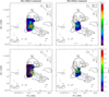 |
Fig. 4 Dust continuum emission at 110 GHz for −2, 3, 5, 7, 10, 30, and 50σ (black contours) superimposed on the ionization fraction maps (top panels) and on the corresponding statistical uncertainties (lower panels) for the blue- and redshifted velocity components (left and right columns, respectively). The spatial scale is shown in the top-right corner of the upper panels. |
5 Discussion
5.1 Local destruction of deuterated molecules
The deuteration fractions observed in Class 0 protostars range between 1% and 10%, with a large scatter from source to source and at the different protostellar scales (Caselli 2002; Roberts et al. 2002; Jørgensen et al. 2004). The [DCO+]/[H13CO+] values that we find for B335 are therefore in broad agreement with the typical range reported in the literature, even accounting for temperature effects. However, Butner et al. (1995) found a [DCO+]/[HCO+] of ≃3% in B335 at scales of ~10000 au. This value is larger than the range of values we find with ALMA at smaller scales, which indicates a decrease in RD toward the center of the envelope. Indeed, RD decreases down to < 1% toward the center and the northern region of the source. This decrease could be attributed to local radiation processes occurring during the protostellar phase, after the protostar has been formed. An increase in the local radiation could promote processes that would lead to the destruction of deuterated molecules due to the evaporation of neutrals to the gas phase (Caselli et al. 1998; Jørgensen et al. 2004), or the increased abundance of ionized molecules like HCO+ (Gaches et al. 2019).
The decreasing trend in RD is further confirmed by our observations of N2D+ (J = 3–2). Figure 7 shows the deuteration map overplotted with the N2D+ (J = 3–2) integrated emission. A lack of N2D+ is observed in regions where RD is lower, suggesting that the physical processes lowering the abundance of O-bearing deuterated molecules also lower the abundance of N-bearing deuterated species around the protostar.
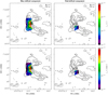 |
Fig. 5 Dust continuum emission at 110 GHz for −2, 3, 5, 7, 10, 30, and 50σ (black contours) superimposed on the ionization rate maps (top panels) and on the corresponding statistical uncertainties (lower panels) for the blue- and redshifted velocity components (left and right columns, respectively). The scale is shown in the top-right corner of the upper panels. |
5.2 High values of C and O depletion in the source
At core scales, observations of the depletion in B335 have been rather inconclusive as some studies suggest very little CO depletion (JCMT 20-arcsec beam probing 3000 au, Murphy et al. 1998), while others suggest a CO depletion of one order of magnitude, fD ~ 10, at similarly large scales (Walmsley & Menten 1987). Our spatially resolved observations reveal large values of CO depletion of the gas in the inner envelope of B335 at radii <1000 au. As shown in Fig. 3, we find fD ranging from 20 to 40 at radii of 1000–100 au, except at the core center where it increases up to 80. Such CO depletion at protostellar radii 100–1000 au is somehow unexpected, if one assumes depletion is due to freeze-out onto dust grains. Indeed, gas and dust at such radii should have temperatures beyond ~20–30 K, where the evaporation of CO from the surface of the dust should replenish it in the gas phase (Anderl et al. 2016). The high depletion values found at the protostar position are highly uncertain due to unknown optical depth, and unconstrained dust and gas temperatures. We stress that the possible depletion increase toward the center in B335 should be confirmed with further observations of higher J transitions of CO.
Several observational studies of protostellar cores have found depletion factors fD > 10 at scales of ~ 5000 au, with some spatially resolved studies pointing to values up to ~ 20 (Alonso-Albi et al. 2010; Christie et al. 2012; Yildiz et al. 2012; Fuente et al. 2012). Models of protostellar evolution with short warm-up timescales in the envelope (see e.g., Aikawa et al. 2012) show that fD may remain high even inside the sublimation radius, especially at early stages, because of the conversion of CO into CH3OH and CH4 on the grain surfaces. Photodissociation due to the protostellar UV radiation could contribute to lowering the global CO abundance in the innermost layers of protostellar envelopes (Visser et al. 2009). Additionally, other sources of ionization, such as CRs, could decrease the abundance of CO in the gas phase by promoting its reaction for the formation of HCO+ (Gaches et al. 2019). This decrease in CO by transformation into HCO+ could also explain the observed coincidence between regions with large CO depletion and low RD.
Another possible cause for the observed depletion could be the presence of relatively large dust grains, as observed in several protostars at similar scales by Galametz et al. (2019). Indeed, larger grains are less efficiently warmed up (Iqbal & Wakelam 2018), limiting the desorption of CO ices to the gas phase. We note that the presence of large dust grains in the inner envelope of B335 could also favor enhanced ionization of the gas (Walmsley et al. 2004), and thus also be consistent with our findings regarding ionization.
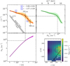 |
Fig. 6 Upper left panel: ζCR as a function of the radius, r. The two dotted black lines at 270 and 500 au identify the radius ranges used to compute the slopes (s1 and s2, respectively). The gray shaded region shows the expected X-ray ionization in the outflow cavity for a typical and a flaring T Tauri star (Rab et al. 2017). Lower left panel: hydrogen column density, |


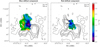 |
Fig. 7 Deuteration fraction maps for the blue- and redshifted velocity components (left and right columns, respectively). The N2D+ (J = 3–2) integrated emission is shown overlaid as black contours at 3, 5, 10, 15, and 20σ, where σ = 5.23 mJy beam−1. The spatial scale is shown in the top-right corners of each panel. |
5.3 Origin of the ionization
From the single-dish observations of Butner et al. (1995), Caselli et al. (1998) find ionization fractions of protostellar gas at core scales of the order of 10−8–10−6. In the B335 outer envelope where n(H2) ~ 104 cm−3, these authors estimate χe of a few 10−6. With our interferometric data, we measure χe ~2 × 10⁻⁶ in the inner envelope, where n(H2) ~ 106 cm−3, with the largest values being χe ~ 9 × 10⁻⁶. We note that while all these aforementioned values are only providing line-of-sight averages for χe, the interferometric data only select a narrow range of spatial scales, making them less sensitive to line-of-sight averaging than single-dish data, and therefore they are more representative of local abundance variations.
We stress that, while the use of deuteration to measure χe is a standard practice in the literature, it has been noted that such an approach may not give accurate results in low-density medium experiencing small deuteration fractions (e.g., ~103 cm−3, Vaupré et al. 2014). In this case, the abundances of DCO+ and HCO+ mostly depend on the ζCR/nH ratio and not only on ζCR, and using RD to get ζCR is valid only when deuteration is > 2%: the measured values in B335 are mostly all lower than this threshold at radii <500 au, which would suggest that our approach of using these observations to derive χe is deficient. However, recent models have shown that in warm dense gas (T ≳ 24 K and nH ~ 106 cm−3), which is typical of the conditions probed here, the relation between RD and ζCR is more robust. Shingledecker et al. (2016) show that the scatter of ζCR predicted by the Caselli model at low ionization values seems to be related to variations in the ortho-to-para ratio (OPR) of H2. While the OPR is an unobservable parameter for dense gas conditions, and therefore cannot be measured for our source, the work of these latter authors shows that the dependence of the relation between RD and ζCR on OPR is weaker for evolved sources due to the stabilization of the OPR. This effect has been shown to happen sooner when nH and the temperature are increased. This was also pointed out by Bron et al. (2021) who show that RD is a robust estimator of ζCR when the gas is subject to high ionization fractions (χe ≳ 3 × 10⁻⁷). As we are probing a dense region of the core with temperatures larger than 20 K and ionization from an embedded source, this supports our use of the Caselli method to measure ζCR.
The large χe values could be produced by local UV and X-ray radiation produced in outflow shocks, altering the chemistry from the molecular content around the shocks (e.g., Viti & Williams 1999; Girart et al. 2002, 2005). However, ionization by far-UV (FUV) photons can be ruled out. Indeed, the maximum energy of FUV photons is around 13 eV, thus below the threshold for ionization of molecular hydrogen (15.44 eV). The second argument is related to the fact that the extinction cross-section at FUV wavelengths (≃0.1 μm) is σUV ≃ 2 × 10⁻²¹ cm2 per hydrogen atom (Draine 2003). Thus, FUV photons are rapidly absorbed in a thin layer of column density equal to (2σUV)−1 ≃ 3 × 1020 cm−2.
The absorption cross-section of X-ray photons, σX, in the range 1–10 keV is much smaller than at FUV frequencies (Bethell & Bergin 2011). For example, at 1 keV and 10 keV, σX ≃ 2 × 10⁻²² cm2 and ≃8 × 10⁻²⁵ cm2 per H atom, respectively.
While at 1 keV the corresponding absorption column density is still small, (2σX)−1 ≃ 2 × 1021 cm−2, at 10 keV it reaches about 6 × 1023 cm−2, much larger than the maximum H2 column density,  , that we found. The latter was computed by integrating the dust continuum at 110 GHz along directions identified by the position angle ϑ (see lower right panel of Fig. 6) and is representative of the column density in the outflow cavity. We therefore estimated the X-ray ionization rate, ζX, using the spectra described by Rab et al. (2017) for a typical and a flaring T Tauri star, assuming a stellar radius of 2R⊙. Results for ζX are shown in the upper left panel of Fig. 6. It is evident that X-ray ionization cannot explain the values of the ionization rate estimated from observations. A fraction of these X-ray photons end up in the disk, which has much higher densities than the cavity, and so
  can easily reach values greater than 1024 cm−2, as found by Grosso et al. (2020) for a Class 0 protostar. At such high
  , ζX decreases dramatically.
Once the high-energy radiation field is excluded as the main source of ionization rate estimated from observations, the only alternative left is CRs (see Sect. 4.3). However, the range of derived values is much higher than those expected from Galactic CRs (see Appendix C in Padovani et al. 2022, for an updated compilation of observational estimates of ζCR). Following McKee (1989), χe = 1.3 × 10⁻⁵n(H2)−1/2, and for the volume densities derived in Sect. 4.3, we should expect χe values of 10−7 to 10−8, which are between one and two orders of magnitude lower than the observed values in B335. As we also observed a significant increase in χe toward the center, and especially of ζCR, the origin of the high values should be of local origin. In particular, we are most likely witnessing the local acceleration of CRs in shocks located in B335 as predicted by theoretical models (Padovani et al. 2015, Padovani et al. 2016, 2020). The values of ζCR found in B335, between about 10−16 and 10−14 s−1, are among the highest values reported in the literature toward star-forming regions (e.g., Maret & Bergin 2007; Ceccarelli et al. 2014b; Fuente et al. 2016; Fontani et al. 2017; Favre et al. 2017; Bialy et al. 2022). We stress that this is the first time that ζCR is measured at such small scales in a solar-type protostar and can be attributed to locally accelerated CRs, as well as the first time that a map of ζCR is obtained.
There are two possible origins for the production of local CRs close to a protostar. One is in strong magnetized shocks along the outflow (Padovani et al. 2015, 2016, 2021; Fitz Axen et al. 2021). Indeed, synchrotron radiation, which is the signature of the presence of relativistic electrons, has been detected in some outflows (Carrasco-González et al. 2010; Ainsworth et al. 2014; Rodríguez-Kamenetzky et al. 2016, 2019; Osorio et al. 2017). The second possibility is in accretion shocks near the stellar surface (Padovani et al. 2016; Gaches & Offner 2018). Both mechanisms are expected to generate low-energy CRs (≲ 100 MeV–30 GeV) through the first-order Fermi acceleration mechanism with a rate of up to ~ 10−13 s−1.
The ionization rate slope found in B335 for r < 270 au is close to −1 and compatible with a diffusive regime, in agreement with predictions of theoretical models. Surprisingly, at radii larger than ~ 250 au, the slope decreases below −2, thus beyond the geometrical dilution regime. We propose two possible explanations. On the one hand, local CRs may have accumulated enough column density to start being thermalized. On the other hand, at radii above about 250 au, both the dust emission and ζCR maps gradually lose their central symmetry (see Figs. 1 and 5, respectively). For example, the continuum map shows two higher density arms toward the northeast and southeast. Therefore, the slope, calculated by averaging over the position angle distribution ϑ, could be less than −2. The loss of symmetry at larger radii in the ionization maps might also be additional evidence as to the importance of non-symmetrical motions during the protostellar collapse (Cabedo et al. 2021). However, we note that these values are also affected by our limited angular resolution of 1.5 arcsec (~250 au), implying that only three or four points in the plot are completely independent, and that observations at larger angular resolution are needed in order to confirm the observed trend.
Previous observations indicate that B335 hosts a powerful and variable jet, which might explain a large production of local CRs (Gâlfalk & Olofsson 2007; Yen et al. 2010). Nevertheless, the exact origin of the local CR source is difficult to pinpoint due to our limited angular resolution. The column density calculated from the dust continuum map at 110 GHz (see lower left panel of Fig. 6) is consistent with that expected in the outflow cavity. To calculate the minimum energy that protons must have in order to pass through a given column density without being thermalized, we can make use of the stopping range function (see Fig. 2 in Padovani et al. 2018). At  cm−2, protons with energies of about 10 MeV are thermalized and lose their ionizing power (see also the upper x-axis of Fig. 6). As discussed above, if the shock is in the vicinity of the protostellar surface, a column density of the order of 1024–1025 cm−2 can easily be accumulated (Grosso et al. 2020). In this case, the minimum proton energy required to prevent thermalization is 100 MeV and 400 MeV at 1024 and 1025 cm−2, respectively. Models of local CR acceleration in low-mass protostars predict that accelerated protons can reach maximum energies of the order of 100 MeV and 10 GeV if the shock in which they are accelerated is located in the jet or close to the protostellar surface, respectively (Padovani et al. 2015, 2016). Thus, although the position of the shock that accelerates these local CRs in B335 is unknown, models suggest that the maximum energies of the protons are sufficiently high to explain the observed ionization.
Additionally, we note that B335 has been observed to exhibit an organized magnetic field at scales similar to the ones probed here (Maury et al. 2018). This could also create favorable conditions for enhanced CR production. Finally, our results are in agreement with CR ionization models on protostellar cores with an embedded radiation source (Gaches et al. 2019); these latter models also suggest that ionization models based solely on  chemistry might underpredict χe by one order of magnitude, except in regions where CR ionization is dominant.
5.4 Magnetic field coupling and non-ideal MHD effects
The ionization fraction of the gas in a young accreting protostar is not only important to understand the early chemistry around solar-type stars, feeding the scales where disks and planets will form, but is also the critical parameter that determines (i) the coupling between the magnetic field and the infalling-rotating gas in the envelope, and (ii) the role of diffusive processes, such as ambipolar diffusion, which counteract the outward transport of angular momentum due to magnetic fields (a process known as magnetic braking). The higher the gas ionization, the more efficient the coupling, and the braking.
The large fraction of ionized gas unveiled by our observations in the inner envelope of B335 should lead to almost perfect coupling of the gas to the local magnetic field lines, generating a drastic braking of rotational motions. We note that these new results lend extra support to other observational evidence of a very efficient magnetic braking at work in B335, notable the highly pinched magnetic field lines observed at similar scales by Maury et al. (2018), and the failure to detect any disk larger than ~ 10 au in this object (Yen et al. 2015); although a new kinematic analysis may be motivated in light of the detection of several velocity components in the accreting gas at scales of ~500 au (Cabedo et al. 2021).
At the end of the pre-stellar stage, the fraction of ionized gas toward the central part of the core is expected to be very low, as Galactic CRs do not penetrate deeply and there is no local ionization source (Padovani & Galli 2013; Ceccarelli et al. 2014a; Silsbee & Ivlev 2019). Hence, the initial stages of protostellar evolution are proceeding under low ionization conditions at typical ζCR < 10−16 s−1 (Padovani et al. 2018; Ivlev et al. 2019), which enhance the importance of non-ideal MHD processes (Padovani et al. 2014), with efficient diffusion of magnetic flux outwards during the very first phases of the collapse, and reduced magnetic braking. If the local ionization processes we observe in B335 are prototypical of solar-type Class 0 protostars, then CRs accelerated in the proximity of the protostar could be responsible for changing the ionization fraction of the gas at disk-forming scales once the protostar is formed, setting quasiideal MHD conditions in the inner envelope. The timescale and magnitude of this transition from non-ideal MHD conditions to quasi-ideal MHD conditions may depend on the protostellar properties: more detailed modeling and observations toward other protostars are required to address this question. Moreover, we note that the observed large χe is not in agreement with the values used to calculate the simplified chemical networks in non-ideal MHD models of protostellar formation and evolution (Marchand et al. 2016; Zhao et al. 2020), as gas ionization is usually predicted from the gas density following McKee (1989). Thus, our observations suggest that careful treatment of ionizing processes in magnetized models may be crucial to properly describe the gas-magnetic field coupling at different scales in embedded protostars.
In this scenario, the properties of protostellar disks could be tightly related to the local acceleration of low-energy CRs, and the development of a highly ionized region around the protostar. Therefore, we would not expect the ionization fraction of the gas present at large scale in the surrounding cloud to be a key factor in setting the disk properties, as proposed for example by Kuffmeier et al. (2020). The scenario we propose is also in agreement with recent ALMA observations of the Class II disks in Orion that do not find supporting evidence of local cloud properties affecting the disk properties (van Terwisga et al. 2022).
6 Conclusions and summary
This work provides new insights into the physico-chemical conditions of the gas in the young Class 0 protostar B335. For the first time, we derived a map of the gas χe and of ζCR at envelope scales < 1000 au in a Class 0 protostar. Our results highlight the interplay between physical processes responsible for gas ionization at disk-forming scales, and its consequences for magnetized models of solar-type star formation. Here, we summarize the main results of our analysis:
We used ALMA data to create molecular line emission maps and used these to characterize the physico-chemical properties of the dense gas in B335. We used the chemical recipe from Caselli et al. (1998) to derive χe based on the deuteration fraction of HCO+ and of the fD. This recipe was recently shown to be valid for dense molecular gas, ~106 cm−3, with a high ionization fraction (≳3 × 10⁻⁷, Bron et al. 2021). It allows us to characterize the ionization of the gas at envelope radii ≲ 1000 au: we find large fractions of ionized gas, χe, between 1 and 8 × 10⁻⁶. These values are remarkably higher than the ones usually measured at core scales.
We produced for the first time a map of ζCR, in the close environment of a young embedded protostar. Our analysis reveals very high values of ζCR between 10−16 and 10−14 s−1, increasing toward the central protostellar embryo at small envelope radii. This suggests that local acceleration of CRs, and not the penetration of interstellar CRs, may be responsible for the gas ionization in the inner envelope, potentially down to disk forming scales.
The large fraction of ionized gas we find suggests an efficient coupling between the magnetic field and the gas in the inner envelope of B335. This interpretation is also supported by the observations of highly organized magnetic field lines, and no detection of a large rotationally supported disk in B335.
If our findings are found to be prototypical of the low-mass star formation process, they might imply that the collapse at scales < 1000 au transitions from non-ideal to a quasi-ideal MHD once the central protostar starts ionizing its surrounding gas, and very efficient magnetic braking of the rotating-infalling protostellar gas might then take place. Protostellar disk properties may therefore be determined by local processes setting the magnetic field coupling, and not only by the amount of angular momentum available at large envelope scales and by the magnetic field strength in protostellar cores. We stress that the gas ionization we find in B335 significantly stands out from the typical values routinely used in state-of-the-art models of protostellar formation and evolution. Our observations suggest that a careful treatment of ionizing processes in these magnetized models may be crucial to properly describe the processes responsible for disk formation and early evolution. We also note that more observations of B335 at higher spatial resolution, and of other Class 0 protostars, are crucial to confirm our results.
Acknowledgments
This project has received funding from the European Research Council (ERC) under the European Union Horizon 2020 research and innovation programme (MagneticYSOs project, grant agreement N° 679937). This work was also partially supported by the program Unidad de Excelencia Maria de Maeztu CEX2020-001058-M. J.M.G. also acknowledges support by the grant PID2020-117710GB-I00 (MCI-AEI-FEDER, UE). Additionally, this paper makes use of the following ALMA data: 2015.1.01188.S. ALMA is a partnership of ESO (representing its member states), NSF (USA) and NINS (Japan), together with NRC (Canada), MOST and ASIAA (Taiwan), and KASI (Republic of Korea), in cooperation with the Republic of Chile. The Joint ALMA Observatory is operated by ESO, AUI/NRAO and NAOJ
Appendix A Technical details of the ALMA observations
Table A.1 presents the technical details of the ALMA observations presented in this work, including the ALMA configuration, the date and time range, the central frequency, the obtained spectral resolution, and the different calibrators used.
Technical details of the ALMA observations.
Appendix B Line profile analysis
B.1 Spectral maps
The DCO+ (J=3-2) and H13CO+ (J=3-2) spectral maps are presented in Figs. B.1 and B.3. Both maps show emission in a region of 5.5″ × 5.5″ (900 au) around the center of the source, with each spectrum corresponding to a pixel of 0.5″ (82 au). The H13CO+ (J=1-0) shows only a region 4″ × 4″ (685 au) and each spectrum corresponds to 0.25″ (41 au).
The three tracers present the same pattern observed in C17O (J=1-0), presented in Cabedo et al. (2021). The line profiles are double-peaked with one of the two velocity components progressively disappearing at different offsets of the source, that is, the blueshifted component is dominant in the eastern region of the source while the redshifted component is present only in the western region. For the three transitions, the blueshifted component is always more intense than the redshifted one, which produces the blue asymmetric morphology observed in the integrated intensity images.
As none of the tracers present a morphology typical of the outflow cavity, we assume that they are not tracing outflowing gas and that the two velocity components are not caused by this effect. This is confirmed with the spectral maps where no signatures coming from outflowing gas —such as very broad lines or high velocity wings— can be observed in the line profiles. This is generally true, except for a small region on the southeast region of the H13CO+ (J=3-2) map, where an additional third velocity component, or “shoulder”, can be observed. This additional component appears to be very broad, and at velocities of ~7.6–7.7 km s−1. We do attribute this signature to outflow contamination, which is observed neither in DCO+ (J=3-2) nor in H13CO+ (J=1-0). We consider that while the outflow might have some effect in the line profiles, this is negligible and is not the main cause of the double-peaked line profiles. The effect of large-scale filtering cannot be ruled out. This is particularly visible in the DCO+ (J=3-2) and H13CO+ (J=3-2) where negative emission is observed in the center and west regions of the source. While these two effects can be a source of uncertainty in our analysis, we conclude that they alone cannot produce the observed line profiles and the velocity pattern through the source, and proceed with the line modeling with the assumption of two independent velocity components.
B.2 Line profile modeling
In this case, as none of the transitions present a resolved hyperfine structure, the opacity of the line could not be obtained by modeling the line profile and only the peak velocity and velocity dispersion maps (as σ) are presented. The resulting maps for DCO+ (J=3-2), H13CO+ (J=1-0), and H13CO+ (J=3-2) are shown in Figs. B.4, B.5, and B.6. For the three tracers, the two separated velocity components occupy different regions of the source, indicating that they are probing gas with different motions. The morphology of the two components is similar for the three tracers, but it is slightly different from the fitting obtained with the C17O (Fig. 5 in Cabedo et al. 2021), where the redshifted component is almost always present in the C17O spectra.
Peak velocity value (top panels of Figs. B.4, B.5 and B.6) ranges are similar for all molecules (from ~8 to 9 km s−1), although the blueshifted component goes to slightly lower velocities for H13CO+ (J=3-2), being the lowest velocities ~7.8 km s−1. This decrease occurs toward the southeastern region of the core, at ~5″ from the center. We attribute this to the presence of the third velocity component produced by outflow contamination observed in Fig. B.3, which produces a bad model of the line profile. No gradient indicating rotation is observed in the velocity maps for any tracer.
Velocity dispersion (bottom panels of Figs. B.4, B.5 and B.6) ranges are also similar for all tracers (from 0.1 to 0.5 km s−1). However, there are some main differences: velocity dispersion is generally larger for H13CO+ (J=3-2) with average values of ~0.4 km s−1, whereas for DCO+ (J=3-2) and H13CO+ (J=1-0) mean values are around ~ 0.25 km s−1. Very large values of the velocity dispersion (>0.5 km s−1) are observed in the same southeastern region of the blueshifted component of H13CO+ (J=3-2) which is a consequence of the poor fitting due to the third velocity component. Values for the velocity dispersion are generally larger for the blueshifted than for the redshifted velocity component, indicating the two components trace gas with different kinematics, i.e., different infall velocities are affected differently by turbulence. For all tracers and both velocity components, the velocity dispersion increases toward the center, as the temperature rises. This increase is smaller for the H13CO+ (J=1-0) emission (up to ~0.35 km s−1) than for the DCO+ (J=3-2), and H13CO+ (J=3-2) (up to ~0.5 km s−1) indicating that H13CO+ (J=1-0) traces gas at colder temperatures and further to the center of the source.
In general, there is good agreement between the values obtained for DCO+ (J=3-2) and H13CO+ (J=3-2), both for peak velocity and velocity components. Considering that we are tracing similar scales, this confirms that both tracers are tracing similar gas. However, C17O presents some differences with respect to H13CO+ (J=1-0) which indicates that they are tracing slightly different gas, C17O tracing warmer and denser gas closer to the protostar.
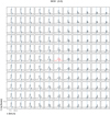 |
Fig. B.1 Spectral map of the DCO+ (J = 3–2) emission in the inner 900 au, centered on the dust continuum emission peak. The whole map is 5.5″ × 5.5″ and each pixel corresponds to 0.5″(~ 82 au). The red spectrum refers to the peak of the continuum emission and the blue line indicates the systemic velocity (8.3 km s−1). |
 |
Fig. B.2 Spectral map of the H13CO+ (J=1–0) emission in the inner 658 au centered on the dust continuum emission peak. The whole map is 4″ × 4″ and each pixel corresponds to 0.25″ (~ 41 au). The red spectrum refers to the peak of the continuum emission, and the blue line indicates the systemic velocity (8.3 km s−1). |
 |
Fig. B.3 Spectral map of the H13CO+ (J = 3–2) emission in the inner 900 au centered on the dust continuum emission peak. The whole map is 5.5″ × 5.5″ and each pixel corresponds to 0.5″(~ 82 au). The red spectrum refers to the peak of the continuum emission and the blue line indicates the systemic velocity (8.3 km s−1) |
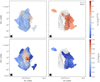 |
Fig. B.4 DCO+ (J=3–2) maps obtained from modeling the line profiles with two velocity components. Overlaid contours show the integrated intensity at −3, 3, 5, 10, and 20 σ. The top map shows values for the peak velocity and bottom show values for the line width (given as σ). Left and right show the blue- and redshifted component, respectively. |
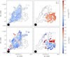 |
Fig. B.5 H13CO+ (J=1–0) maps obtained from modeling the line profiles with two velocity components. Overlaid contours show the integrated intensity at −3, 3, 5, and 10 σ. The top map shows values for the peak velocity and bottom show values for the line width (given as σ). Left and right show the blue- and redshifted component, respectively. |
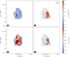 |
Fig. B.6 H13CO+ (J=3–2) maps obtained from modeling the line profiles with two velocity components. Overlaid contours show the integrated intensity at −3, 3, 5, 10, and 20 σ. The top map shows values for the peak velocity and bottom show values for the line width (given as σ). Left and right show the blue- and redshifted component, respectively. |
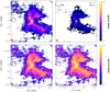 |
Fig. C.1 Expected optical depth maps for the four molecular tracers (see text in Section C for details). Top left: C17O (J=1–0). Top right: DCO+ (J=3–2). Bottom left: H13CO+ (J=1–0). Bottom right: H13CO+ (J=3–2). |
Appendix C Estimation of the opacity effects
As the line profile modeling does not allow us to obtain the line opacities, we estimated the optical depth using the dust continuum emission and the molecular abundances in order to determine the impact on the parameters derived from the line modeling. We first compute the H2 column density map from the dust continuum emission map at 110 GHz (shown in Fig. 1), assuming its emission is optically thin (e.g., tracing the full column density) and applying the following standard abundances: [C17O] = 5×10⁻⁸ (Thomas & Fuller 2008), [DCO+] = 10−11 and [H13CO+] = 10−10 (Jørgensen et al. 2004). Figure C.1 shows the expected optical depth maps for the four different molecular lines we obtain with this method. Values of the optical depth are generally low (< 1), although they increase to larger values for all tracers in the central beam. We note that, as we are considering a constant temperature for the derivation of the H2 column density, which is likely higher at the center, the H2 column density values in the central compact source are probably smaller, and we are overestimating the optical depth in that region. It can be seen that both transitions of H13CO+ present larger values of optical depth than both C17O (J=1-0) and DCO+ (J=3-2). We acknowledge that these large values can potentially affect our deuteration measurements toward the central beam, but stress that the small optical depth values found in DCO+ confirm that the two velocity components are not mainly produced by self-absorption effects. Outside of that central beam, the expected line opacities are generally smaller than 1, so we found no need for applying an opacity correction to our data.
References
- Aikawa, Y., Wakelam, V., Hersant, F., Garrod, R. T., & Herbst, E. 2012, ApJ, 760, 40 [NASA ADS] [CrossRef] [Google Scholar]
- Ainsworth, R. E., Scaife, A. M. M., Ray, T. P., et al. 2014, ApJ, 792, L18 [Google Scholar]
- Alonso-Albi, T., Fuente, A., Crimier, N., et al. 2010, A&A, 518, A52 [NASA ADS] [CrossRef] [EDP Sciences] [Google Scholar]
- Alves, F. O., Frau, P., Girart, J. M., et al. 2014, A&A, 569, A1 [NASA ADS] [CrossRef] [EDP Sciences] [Google Scholar]
- Anderl, S., Maret, S., Cabrit, S., et al. 2016, A&A, 591, A3 [NASA ADS] [CrossRef] [EDP Sciences] [Google Scholar]
- Asayama, S., Biggs, A., de Gregorio, I., et al. 2016, ALMA Partnership [Google Scholar]
- Bethell, T. J., & Bergin, E. A. 2011, ApJ, 740, 7 [NASA ADS] [CrossRef] [Google Scholar]
- Bialy, S., Belli, S., & Padovani, M. 2022, A&A, 658, A13 [Google Scholar]
- Bron, E., Roueff, E., Gerin, M., et al. 2021, A&A, 645, A28 [NASA ADS] [CrossRef] [EDP Sciences] [Google Scholar]
- Butner, H. M., Lada, E. A., & Loren, R. B. 1995, ApJ, 448, 207 [NASA ADS] [CrossRef] [Google Scholar]
- Cabedo, V., Maury, A., Girart, J. M., & Padovani, M. 2021, A&A, 653, A166 [NASA ADS] [CrossRef] [EDP Sciences] [Google Scholar]
- Carrasco-González, C., Rodríguez, L. F., Anglada, G., et al. 2010, Science, 330, 1209 [CrossRef] [Google Scholar]
- Caselli, P. 2002, Planet. Space Sci., 50, 1133 [NASA ADS] [CrossRef] [Google Scholar]
- Caselli, P., Walmsley, C. M., Terzieva, R., & Herbst, E. 1998, ApJ, 499, 234 [Google Scholar]
- Ceccarelli, C., Caselli, P., Bockelée-Morvan, D., et al. 2014a, in Protostars and Planets VI, eds. H. Beuther, R. S. Klessen, C. P. Dullemond, & T. Henning, 859 [Google Scholar]
- Ceccarelli, C., Dominik, C., López-Sepulcre, A., et al. 2014b, ApJ, 790, L1 [Google Scholar]
- Christie, H., Viti, S., Yates, J., et al. 2012, MNRAS, 422, 968 [NASA ADS] [CrossRef] [Google Scholar]
- Dapp, W. B., Basu, S., & Kunz, M. W. 2012, A&A, 541, A35 [NASA ADS] [CrossRef] [EDP Sciences] [Google Scholar]
- Draine, B. T. 2003, ARA&A, 41, 241 [NASA ADS] [CrossRef] [Google Scholar]
- Estalella, R. 2017, PASP, 129, 025003 [NASA ADS] [CrossRef] [Google Scholar]
- Evans, Neal J. I., Di Francesco, J., Lee, J.-E., et al. 2015, ApJ, 814, 22 [CrossRef] [Google Scholar]
- Favre, C., López-Sepulcre, A., Ceccarelli, C., et al. 2017, A&A, 608, A82 [NASA ADS] [CrossRef] [EDP Sciences] [Google Scholar]
- Fitz Axen, M., Offner, S. S. S., Gaches, B. A. L., et al. 2021, ApJ, 915, 43 [NASA ADS] [CrossRef] [Google Scholar]
- Fontani, F., Ceccarelli, C., Favre, C., et al. 2017, A&A, 605, A57 [NASA ADS] [CrossRef] [EDP Sciences] [Google Scholar]
- Fuente, A., Caselli, P., McCoey, C., et al. 2012, A&A, 540, A75 [NASA ADS] [CrossRef] [EDP Sciences] [Google Scholar]
- Fuente, A., Cernicharo, J., Roueff, E., et al. 2016, A&A, 593, A94 [NASA ADS] [CrossRef] [EDP Sciences] [Google Scholar]
- Gaches, B. A. L., & Offner, S. S. R. 2018, ApJ, 861, 87 [NASA ADS] [CrossRef] [Google Scholar]
- Gaches, B. A. L., Offner, S. S. R., & Bisbas, T. G. 2019, ApJ, 878, 105 [NASA ADS] [CrossRef] [Google Scholar]
- Galametz, M., Maury, A. J., Valdivia, V., et al. 2019, A&A, 632, A5 [NASA ADS] [CrossRef] [EDP Sciences] [Google Scholar]
- Gâlfalk, M., & Olofsson, G. 2007, A&A, 475, 281 [CrossRef] [EDP Sciences] [Google Scholar]
- Gerner, T., Beuther, H., Semenov, D., et al. 2014, A&A, 563, A97 [NASA ADS] [CrossRef] [EDP Sciences] [Google Scholar]
- Girart, J. M., Viti, S., Williams, D. A., Estalella, R., & Ho, P. T. P. 2002, A&A, 388, 1004 [NASA ADS] [CrossRef] [EDP Sciences] [Google Scholar]
- Girart, J. M., Viti, S., Estalella, R., & Williams, D. A. 2005, A&A, 439, 601 [NASA ADS] [CrossRef] [EDP Sciences] [Google Scholar]
- Girart, J. M., Rao, R., & Marrone, D. P. 2006, Science, 313, 812 [Google Scholar]
- Grosso, N., Hamaguchi, K., Principe, D. A., & Kastner, J. H. 2020, A&A, 638, A4 [NASA ADS] [CrossRef] [EDP Sciences] [Google Scholar]
- Hennebelle, P., & Inutsuka, S.-I. 2019, Front. Astron. Space Sci., 6, 5 [NASA ADS] [CrossRef] [Google Scholar]
- Hennebelle, P., Commerçon, B., Lee, Y.-N., & Charnoz, S. 2020, A&A, 635, A67 [NASA ADS] [CrossRef] [EDP Sciences] [Google Scholar]
- Hirano, N., Kameya, O., Kasuga, T., & Umemoto, T. 1992, ApJ, 390, L85 [NASA ADS] [CrossRef] [Google Scholar]
- Hirano, N., Kameya, O., Nakayama, M., & Takakubo, K. 1988, ApJ, 327, L69 [NASA ADS] [CrossRef] [Google Scholar]
- Iqbal, W., & Wakelam, V. 2018, A&A, 615, A20 [NASA ADS] [CrossRef] [EDP Sciences] [Google Scholar]
- Ivlev, A. V., Silsbee, K., Sipilä, O., & Caselli, P. 2019, ApJ, 884, 176 [Google Scholar]
- Jørgensen, J. K., Schöier, F. L., & van Dishoeck, E. F. 2004, A&A, 416, 603 [Google Scholar]
- Keene, J., Davidson, J. A., Harper, D. A., et al. 1983, ApJ, 274, L43 [NASA ADS] [CrossRef] [Google Scholar]
- Kuffmeier, M., Zhao, B., & Caselli, P. 2020, A&A, 639, A86 [NASA ADS] [CrossRef] [EDP Sciences] [Google Scholar]
- Kurono, Y., Saito, M., Kamazaki, T., Morita, K.-I., & Kawabe, R. 2013, ApJ, 765, 85 [NASA ADS] [CrossRef] [Google Scholar]
- Lebreuilly, U., Hennebelle, P., Colman, T., et al. 2021, ApJ, 917, L10 [NASA ADS] [CrossRef] [Google Scholar]
- Li, Z.-Y., Krasnopolsky, R., & Shang, H. 2011, ApJ, 738, 180 [Google Scholar]
- Machida, M. N., Inutsuka, S.-I., & Matsumoto, T. 2011, PASJ, 63, 555 [NASA ADS] [CrossRef] [Google Scholar]
- Marchand, P., Masson, J., Chabrier, G., et al. 2016, A&A, 592, A18 [NASA ADS] [CrossRef] [EDP Sciences] [Google Scholar]
- Marchand, P., Tomida, K., Tanaka, K. E. I., Commerçon, B., & Chabrier, G. 2020, ApJ, 900, 180 [CrossRef] [Google Scholar]
- Maret, S., & Bergin, E. A. 2007, ApJ, 664, 956 [Google Scholar]
- Masson, J., Chabrier, G., Hennebelle, P., Vaytet, N., & Commerçon, B. 2016, A&A, 587, A32 [NASA ADS] [CrossRef] [EDP Sciences] [Google Scholar]
- Maury, A. J., Girart, J. M., Zhang, Q., et al. 2018, MNRAS, 477, 2760 [Google Scholar]
- Maury, A. J., André, P., Testi, L., et al. 2019, A&A, 621, A76 [NASA ADS] [CrossRef] [EDP Sciences] [Google Scholar]
- McKee, C. F. 1989, ApJ, 345, 782 [NASA ADS] [CrossRef] [Google Scholar]
- Murphy, B. T., Little, L. T., & Kelly, M. L. 1998, MNRAS, 294, 635 [NASA ADS] [CrossRef] [Google Scholar]
- Osorio, M., Díaz-Rodríguez, A. K., Anglada, G., et al. 2017, ApJ, 840, 36 [Google Scholar]
- Ossenkopf, V., & Henning, T. 1994, A&A, 291, 943 [NASA ADS] [Google Scholar]
- Padovani, M., & Galli, D. 2013, in Ap&SS Proc., 34, 61 [NASA ADS] [Google Scholar]
- Padovani, M., Galli, D., Hennebelle, P., Commerçon, B., & Joos, M. 2014, A&A, 571, A33 [NASA ADS] [CrossRef] [EDP Sciences] [Google Scholar]
- Padovani, M., Hennebelle, P., Marcowith, A., & Ferrière, K. 2015, A&A, 582, A13 [Google Scholar]
- Padovani, M., Marcowith, A., Hennebelle, P., & Ferrière, K. 2016, A&A, 590, A8 [NASA ADS] [CrossRef] [EDP Sciences] [Google Scholar]
- Padovani, M., Ivlev, A. V., Galli, D., & Caselli, P. 2018, A&A, 614, A111 [NASA ADS] [CrossRef] [EDP Sciences] [Google Scholar]
- Padovani, M., Ivlev, A. V., Galli, D., et al. 2020, Space Sci. Rev., 216, 29 [CrossRef] [Google Scholar]
- Padovani, M., Marcowith, A., Galli, D., Hunt, L. K., & Fontani, F. 2021, A&A, 649, A149 [NASA ADS] [CrossRef] [EDP Sciences] [Google Scholar]
- Padovani, M., Bialy, S., Galli, D., et al. 2022, A&A, 658, A189 [NASA ADS] [CrossRef] [EDP Sciences] [Google Scholar]
- Rab, C., Güdel, M., Padovani, M., et al. 2017, A&A, 603, A96 [NASA ADS] [CrossRef] [EDP Sciences] [Google Scholar]
- Roberts, H., Fuller, G. A., Millar, T. J., Hatchell, J., & Buckle, J. V. 2002, A&A, 381, 1026 [CrossRef] [EDP Sciences] [Google Scholar]
- Rodríguez-Kamenetzky, A., Carrasco-González, C., Araudo, A., et al. 2016, ApJ, 818, 27 [CrossRef] [Google Scholar]
- Rodríguez-Kamenetzky, A., Carrasco-González, C., González-Martín, O., et al. 2019, MNRAS, 482, 4687 [CrossRef] [Google Scholar]
- Shingledecker, C. N., Bergner, J. B., Le Gal, R., et al. 2016, ApJ, 830, 151 [NASA ADS] [CrossRef] [Google Scholar]
- Silsbee, K., & Ivlev, A. V. 2019, ApJ, 879, 14 [NASA ADS] [CrossRef] [Google Scholar]
- Soler, J. D. 2019, A&A, 629, A96 [NASA ADS] [CrossRef] [EDP Sciences] [Google Scholar]
- Stutz, A. M., Rubin, M., Werner, M. W., et al. 2008, ApJ, 687, 389 [NASA ADS] [CrossRef] [Google Scholar]
- Thomas, H. S., & Fuller, G. A. 2008, A&A, 479, 751 [NASA ADS] [CrossRef] [EDP Sciences] [Google Scholar]
- van Terwisga, S. E., Hacar, A., van Dishoeck, E. F., Oonk, R., & Portegies Zwart, S. 2022, A&A 661, A53 [NASA ADS] [CrossRef] [EDP Sciences] [Google Scholar]
- Vaupré, S., Hily-Blant, P., Ceccarelli, C., et al. 2014, A&A, 568, A50 [NASA ADS] [CrossRef] [EDP Sciences] [Google Scholar]
- Visser, R., van Dishoeck, E. F., & Black, J. H. 2009, A&A, 503, 323 [NASA ADS] [CrossRef] [EDP Sciences] [Google Scholar]
- Viti, S., & Williams, D. A. 1999, MNRAS, 310, 517 [NASA ADS] [CrossRef] [Google Scholar]
- Walmsley, C. M., & Menten, K. M. 1987, in Circumstellar Matter, eds. I. Appenzeller, & C. Jordan, 122, 71 [NASA ADS] [CrossRef] [Google Scholar]
- Walmsley, C. M., Flower, D. R., & Pineau des Forêts, G. 2004, A&A, 418, 1035 [NASA ADS] [CrossRef] [EDP Sciences] [Google Scholar]
- Watson, D. M. 2020, RNAAS, 4, 88 [NASA ADS] [Google Scholar]
- Wilson, T. L., & Rood, R. 1994, ARA&A, 32, 191 [Google Scholar]
- Wootten, A. 1987, in Astrochemistry, eds. M. S. Vardya, & S. P. Tarafdar, 120, 311 [NASA ADS] [CrossRef] [Google Scholar]
- Wouterloot, J. G. A., Henkel, C., Brand, J., & Davis, G. R. 2008, A&A, 487, 237 [NASA ADS] [CrossRef] [EDP Sciences] [Google Scholar]
- Yen, H.-W., Takakuwa, S., & Ohashi, N. 2010, ApJ, 710, 1786 [NASA ADS] [CrossRef] [Google Scholar]
- Yen, Takakuwa, S., Koch, P. M., et al. 2015, ApJ, 812, 129 [NASA ADS] [CrossRef] [Google Scholar]
- Yıldız, U. A., Kristensen, L. E., van Dishoeck, E. F., et al. 2012, A&A, 542, A86 [NASA ADS] [CrossRef] [EDP Sciences] [Google Scholar]
- Zhang, Q., Qiu, K., Girart, J. M., et al. 2014, ApJ, 792, 116 [Google Scholar]
- Zhao, B., Caselli, P., Li, Z.-Y., et al. 2020, MNRAS, 492, 3375 [Google Scholar]
- Zhou, S., Evans, I., Neal, J., Koempe, C., & Walmsley, C. M. 1993, ApJ, 404, 232 [NASA ADS] [CrossRef] [Google Scholar]
All Tables
All Figures
|
Fig. 1 Map of the dust continuum emission at 110 GHz clipped for values smaller than 3σ (see Table 1) and integrated emission for the four molecular lines as indicated in the upper left corner (red contours). Contours are −2, 3, 5, 8, 11, 14, and 17σ (the individual σ values are indicated in Table 1). The velocity ranges used to obtain the integrated intensity maps are shown in Table 1. In the bottom-left of each plot, we show the beam size for each molecular line (in red) and for the dust continuum emission (in black). The physical scale is shown in the top-right corner of the figure. |
| In the text | |
|
Fig. 2 Dust continuum emission at 110 GHz for −2, 3, 5, 7, 10, 30, and 50σ (black contours) superimposed on the deuteration fraction maps (top panels) and on the corresponding statistical uncertainties (lower panels) for the blue- and redshifted velocity components (left and right columns, respectively). The spatial scale is shown in the top-right corner of the upper panels. |
| In the text | |
|
Fig. 3 Map of the CO depletion factor and contours of dust continuum emission at 110 GHz, for emission over 3σ. The spatial scale is shown in the top-right corner of the figure. |
| In the text | |
|
Fig. 4 Dust continuum emission at 110 GHz for −2, 3, 5, 7, 10, 30, and 50σ (black contours) superimposed on the ionization fraction maps (top panels) and on the corresponding statistical uncertainties (lower panels) for the blue- and redshifted velocity components (left and right columns, respectively). The spatial scale is shown in the top-right corner of the upper panels. |
| In the text | |
|
Fig. 5 Dust continuum emission at 110 GHz for −2, 3, 5, 7, 10, 30, and 50σ (black contours) superimposed on the ionization rate maps (top panels) and on the corresponding statistical uncertainties (lower panels) for the blue- and redshifted velocity components (left and right columns, respectively). The scale is shown in the top-right corner of the upper panels. |
| In the text | |
|
Fig. 6 Upper left panel: ζCR as a function of the radius, r. The two dotted black lines at 270 and 500 au identify the radius ranges used to compute the slopes (s1 and s2, respectively). The gray shaded region shows the expected X-ray ionization in the outflow cavity for a typical and a flaring T Tauri star (Rab et al. 2017). Lower left panel: hydrogen column density, |
| In the text | |
|
Fig. 7 Deuteration fraction maps for the blue- and redshifted velocity components (left and right columns, respectively). The N2D+ (J = 3–2) integrated emission is shown overlaid as black contours at 3, 5, 10, 15, and 20σ, where σ = 5.23 mJy beam−1. The spatial scale is shown in the top-right corners of each panel. |
| In the text | |
|
Fig. B.1 Spectral map of the DCO+ (J = 3–2) emission in the inner 900 au, centered on the dust continuum emission peak. The whole map is 5.5″ × 5.5″ and each pixel corresponds to 0.5″(~ 82 au). The red spectrum refers to the peak of the continuum emission and the blue line indicates the systemic velocity (8.3 km s−1). |
| In the text | |
|
Fig. B.2 Spectral map of the H13CO+ (J=1–0) emission in the inner 658 au centered on the dust continuum emission peak. The whole map is 4″ × 4″ and each pixel corresponds to 0.25″ (~ 41 au). The red spectrum refers to the peak of the continuum emission, and the blue line indicates the systemic velocity (8.3 km s−1). |
| In the text | |
|
Fig. B.3 Spectral map of the H13CO+ (J = 3–2) emission in the inner 900 au centered on the dust continuum emission peak. The whole map is 5.5″ × 5.5″ and each pixel corresponds to 0.5″(~ 82 au). The red spectrum refers to the peak of the continuum emission and the blue line indicates the systemic velocity (8.3 km s−1) |
| In the text | |
|
Fig. B.4 DCO+ (J=3–2) maps obtained from modeling the line profiles with two velocity components. Overlaid contours show the integrated intensity at −3, 3, 5, 10, and 20 σ. The top map shows values for the peak velocity and bottom show values for the line width (given as σ). Left and right show the blue- and redshifted component, respectively. |
| In the text | |
|
Fig. B.5 H13CO+ (J=1–0) maps obtained from modeling the line profiles with two velocity components. Overlaid contours show the integrated intensity at −3, 3, 5, and 10 σ. The top map shows values for the peak velocity and bottom show values for the line width (given as σ). Left and right show the blue- and redshifted component, respectively. |
| In the text | |
|
Fig. B.6 H13CO+ (J=3–2) maps obtained from modeling the line profiles with two velocity components. Overlaid contours show the integrated intensity at −3, 3, 5, 10, and 20 σ. The top map shows values for the peak velocity and bottom show values for the line width (given as σ). Left and right show the blue- and redshifted component, respectively. |
| In the text | |
|
Fig. C.1 Expected optical depth maps for the four molecular tracers (see text in Section C for details). Top left: C17O (J=1–0). Top right: DCO+ (J=3–2). Bottom left: H13CO+ (J=1–0). Bottom right: H13CO+ (J=3–2). |
| In the text | |
Current usage metrics show cumulative count of Article Views (full-text article views including HTML views, PDF and ePub downloads, according to the available data) and Abstracts Views on Vision4Press platform.
Data correspond to usage on the plateform after 2015. The current usage metrics is available 48-96 hours after online publication and is updated daily on week days.
Initial download of the metrics may take a while.