| Issue |
A&A
Volume 669, January 2023
|
|
|---|---|---|
| Article Number | A3 | |
| Number of page(s) | 24 | |
| Section | Interstellar and circumstellar matter | |
| DOI | https://doi.org/10.1051/0004-6361/202243240 | |
| Published online | 23 December 2022 | |
Using debris disk observations to infer substellar companions orbiting within or outside a parent planetesimal belt
1
Institut für Theoretische Physik und Astrophysik, Christian-Albrechts-Universität zu Kiel,
Leibnizstr. 15,
24118
Kiel, Germany
e-mail: This email address is being protected from spambots. You need JavaScript enabled to view it.
2
Astrophysikalisches Institut und Universitätssternwarte, Friedrich-Schiller-Universität Jena,
Schillergässchen 2-3,
07745
Jena, Germany
Received:
1
February
2022
Accepted:
2
October
2022
Abstract
Context. Alongside a debris disk, substellar companions often exist in the same system. The companions influence the dust dynamics via their gravitational potential.
Aims. We analyze whether the effects of secular perturbations, originating from a substellar companion, on the dust dynamics can be investigated with spatially resolved observations.
Methods. We numerically simulated the collisional evolution of narrow and eccentric cold planetesimal belts around a star of spectral type A3 V that are secularly perturbed by a substellar companion that orbits either closer to or farther from the star than the belt. Our model requires a perturber on an eccentric orbit (e ≳ 0.3) that is both far from and more massive than the collisionally dominated belt around a luminous central star. Based on the resulting spatial dust distributions, we simulated spatially resolved maps of their surface brightness in the K, N, and Q bands and at wavelengths of 70 µm and 1300 µm.
Results. Assuming a nearby debris disk seen face-on, we find that the surface brightness distribution varies significantly with observing wavelength, for example between the N and Q band. This can be explained by the varying relative contribution of the emission of the smallest grains near the blowout limit. The orbits of both the small grains that form the halo and the large grains close to the parent belt precess due to the secular perturbations induced by a substellar companion orbiting inward of the belt. The halo, being composed of older grains, trails the belt. The magnitude of the trailing decreases with increasing perturber mass and hence with increasing strength of the perturbations. We recovered this trend in synthetic maps of surface brightness by fitting ellipses to lines of constant brightness. Systems with an outer perturber do not show a uniform halo precession since the orbits of small grains are strongly altered. We identified features of the brightness distributions suitable for distinguishing between systems with a potentially detectable inner or outer perturber, especially with a combined observation with JWST/MIRI in the Q band tracing small grain emission and with ALMA at millimeter wavelengths tracing the position of the parent planetesimal belt.
Key words: planet–disk interactions / circumstellar matter / interplanetary medium / infrared: planetary systems / submillimeter: planetary systems / methods: numerical
© The Authors 2022
 Open Access article, published by EDP Sciences, under the terms of the Creative Commons Attribution License (https://creativecommons.org/licenses/by/4.0), which permits unrestricted use, distribution, and reproduction in any medium, provided the original work is properly cited.
This article is published in open access under the Subscribe-to-Open model. This email address is being protected from spambots. You need JavaScript enabled to view it. to support open access publication.
1 Introduction
Various close-by main-sequence stars with debris disks have been found to host exoplanets, for example, β Pictoris (Lagrange et al. 2009, 2010, 2019; Nowak et al. 2020), є Eridani (Hatzes et al. 2000), or AU Microscopii (Plavchan et al. 2020; Martioli et al. 2021). Several techniques, direct and indirect, were used to detect the aforementioned exoplanets: the exoplanets β Pic c and є Eri b were inferred by measuring the radial velocity of the host star (Struve 1952); AU Mic b and c were detected by measuring the light curve of the host star while the planet transits the line of sight (e.g., Struve 1952; Deeg & Alonso 2018); and β Pic b and c were detected by direct imaging (Bowler 2016). The first two techniques are sensitive to planets orbiting relatively close to the host star: for the radial velocity method, planets with long orbital periods are difficult to detect because the amplitude of the radial velocity signal decreases with increasing distance between the planet and the host star and due to the sheer time span required to observationally cover an orbit (e.g., Lovis & Fischer 2010); for the transit method, the larger the orbit of a planet, the smaller the angular cross section the planet is blocking in front of the star and the less likely a sufficient alignment of the host star, the orbiting planet, and the observer is. The technique of direct imaging is capable of finding substellar companions on larger orbits, ≳100 au, but requires the planets to still be intrinsically bright and to not have cooled down since formation. This, as such, favors young systems as targets, that is, T Tauri and Herbig Ae/Be stars as well as young moving group members (Bowler 2016); older, already cooled planets are difficult to detect. Astrometry that uses the data obtained by Gaia (Gaia Collaboration et al. 2016) is expected to add thousands of exoplanet detections, but the orbital period of the planets discovered is limited by the mission lifetime of approximately 10 yr (Casertano et al. 2008; Perryman et al. 2014; Ranalli et al. 2018). An exoplanet hunting method without these biases is gravitational microlensing (e.g., Mao & Paczynski 1991; Gould & Loeb 1992; Mao 2012; Tsapras 2018), but with this method systems at distances on the order of kiloparsecs are probed, too distant to be spatially resolved. In summary, we lack a planet hunting method to find old, and hence intrinsically dark, far-out planets in close-by stellar systems.
In addition to exoplanets, stars have often been found to host debris disks (e.g., Maldonado et al. 2012, 2015; Marshall et al. 2014), a common component in stellar systems beyond the proto-planetary phase (e.g., Su et al. 2006; Eiroa et al. 2013; Montesinos et al. 2016; Sibthorpe et al. 2018). They are produced and continuously replenished by mutually colliding planetesimals that grind themselves down to dust in a collisional cascade and are characterized as being optically thin (for recent reviews, see Matthews et al. 2014; Hughes et al. 2018; Wyatt 2020). The disks are usually observed in the near-infrared via the stellar light scattered off the dust and in the mid-infrared, far-infrared, and (sub)millimeter wavelength range via the thermal emission of the dust itself.
Planets orbiting in a debris disk system have an impact on the planetesimal and dust grain dynamics via their gravitational potential. Therefore, by observing the dust emission one can potentially draw conclusions regarding the possibly unseen planets orbiting the central star (e.g., Wyatt et al. 1999; Wolf et al. 2007; Krivov 2010; Lee & Chiang 2016). The strength of the perturbing effect that a substellar companion has on the orbits of planetesimals and dust primarily depends on the distance of the perturber to the perturbed objects. Therefore, the spatial dust distribution produced by planetesimal collisions can be a signpost of old and far-out planets as well. Hence, analyses of spatially resolved observations of debris disks potentially serve as a planet hunting method that is complementary to the well-established methods that make use of stellar radial velocity, transits, and direct imaging to find exoplanets in close-by stellar systems (e.g., Pearce et al. 2022).
Narrow, eccentric debris rings are particularly promising tracers of long-term planetary perturbations. The deviation from circularity suggests that perturbations have happened, while the narrowness excludes violent short-term causes such as stellar flybys (e.g., Larwood & Kalas 2001; Kobayashi & Ida 2001) or (repeated) close encounters with planets (e.g., Gomes et al. 2005). For long-term perturbations, where timescales are much longer than individual orbital periods, the orbits of belt objects are affected more coherently, with little spread in orbital elements. In contrast, instantaneous positions along the orbits are important in short-term perturbation events, resulting in a wider spread in orbital elements and wider disks. A narrow yet eccentric disk can only be compatible with a disk-crossing planet if the thus-excited wide disk component is subsequently removed (Pearce et al. 2021). The belts around Fomalhaut (e.g., Kalas et al. 2005, 2013; Boley et al. 2012; MacGregor et al. 2017), HD 202628 (Krist et al. 2012; Schneider et al. 2016; Faramaz et al. 2019), HD 53143 (MacGregor et al. 2022), and the younger system HR 4796 A (e.g., Moerchen et al. 2011; Kennedy et al. 2018) are well-resolved examples of narrow, eccentric disks.
To accomplish the task of using spatially resolved observations of dust emission to infer exoplanets and their properties, two key ingredients are necessary: first, the planet-disk interaction, that is, how perturbing planets shape the spatial dust distributions, and second, how these dust distributions appear in observations. With such a framework, in addition to searching for hints of exoplanets, we can use the known exoplanet–debris disk systems as test beds to better constrain debris disk properties such as collisional timescales, planetesimal stirring (e.g., Marino 2021), or self-gravitation (Sefilian et al. 2021) as well as planetesimal and dust material properties such as the critical energy for fragmentation, Q*D (e.g., Kim et al. 2018).
This paper is organized as follows: In Sect. 2, we present the numerical methods applied to collisionally evolve planetesimal belts secularly perturbed by a substellar companion and discuss the resulting spatial grain distributions for different perturber–belt combinations. Based on these results, we show in Sect. 3 how we simulated surface brightness distributions and explore the relative contribution of different grain sizes to the total radiation as well as how the halo of small grains on very eccentric orbits can be investigated observationally. In Sect. 4, we search for observable features to distinguish between systems with a substellar companion orbiting inside or outside a parent planetesimal belt and present our results in a simple decision tree. Lastly, in Sect. 5 we discuss the results and in Sect. 6 briefly summarize our findings.
2 ACE simulations
We used the code Analysis of Collisional Evolution (ACE, Krivov et al. 2005, 2006; Vitense et al. 2010; Löhne et al. 2017; Sende & Löhne 2019) to evolve the radial, azimuthal, and size distribution of the material in debris disks. ACE follows a statistical approach, grouping particles in category bins according to their masses, m, and three orbital elements: pericenter distances, q, eccentricities, e, and longitudes of periapse, ϖ = Ω + ω.
Mutual collisions can lead to four different outcomes in ACE, depending on the masses and relative velocities of the colliders. At the highest impact energies, both colliders are shattered and the fragments dispersed such that the largest remaining fragment has less than half the original mass. Below the energy threshold for disruption and dispersal, a larger fragment remains, either as a direct remnant of the bigger object or as a consequence of gravitational re-accumulation. A cloud of smaller fragments is produced. If neither of the two colliders is shattered by the impact, both were assumed to rebound, resulting in two large remnants and a fragment cloud. In the unreached case of an impact velocity below ~1 m s−1, the colliders would stick. These four regimes assumed in ACE represent a simplification of the zoo of outcomes mapped by Güttler et al. (2010). In addition to the collisional cascade, we took into account stellar radiation and wind pressure, the accompanying drag forces, and secular gravitational perturbation by a substellar companion.
In the following subsections, we describe the recent improvements made to the ACE code, motivate and detail the simulation parameters, and present the resulting distributions.
2.1 Improved advection scheme
In Vitense et al. (2010) and subsequent work (e.g., Reidemeister et al. 2011; Schüppler et al. 2014; Löhne et al. 2017), we used the upwind advection scheme to propagate material through the q–e grid of orbital elements under the influence of Poynting–Robertson (PR) and stellar wind drag. Sende & Löhne (2019) applied that scheme to the modeling of secular perturbations, where q, e, and ϖ are affected while the semimajor axes are constant. In the following we refer to both PR drag and secular perturbations as transport.
The upwind scheme moves material across the borders from one bin to its neighbors based on the coordinate velocities and amount of material in that bin. The scheme is linear in time and has the advantage that the transport gains and losses can be added simply to the collisional ones. For the PR effect, where drag leads to smooth and monotonous inward spread and circularization from the parent belt and halo, this scheme is sufficient. However, a narrow, eccentric parent belt under the influence of (periodic) secular perturbations requires the translation of sharp features in q, e, and ϖ across the grid. The upwind scheme smears the sharp features out too quickly, inducing an unwanted widening and dynamical excitation of the disk (Sende & Löhne 2019). To reduce the effect of this numerical dispersion, we introduced an operator splitting to the ACE code, where collisions and transport (caused by drag and secular perturbation) are integrated one after the other for every time step. The transport part is integrated using a total variance diminishing (TVD) scheme (Harten 1983) with the superbee flux limiter (Roe 1986). The contributions from PR drag and secular perturbation to the change rates  , and
, and  are summed up. For each time step ∆t, the flow in three dimensions is again subdivided into five stages: ∆t/2 in q, ∆t/2 in e, ∆t in ϖ, ∆t/2 in e, and ∆t/2 in q. A comparison of the resulting amounts of numerical dispersion in the TVD and the upwind schemes is shown in Appendix A.
2.2 Common parameters
The distribution of observable dust grains is determined by a range of parameters, including not only parameters of the dust, the disk, and the perturber, but also of the host star. The dust material was not varied in our study as we deem the discussed tracers of planetary perturbations unaffected. We chose a material blend of equal volume fractions of water ice Li & Greenberg (1998) and astronomical silicate (Draine 2003), assuming a bulk density of 2.35 g cm−3 for the blend. The refractive indices are combined with the Maxwell–Garnett mixing rule (Garnett 1904). Radiation pressure efficiency as well as absorption and scattering cross sections were calculated assuming compact spheres, using the Mie theory (Mie 1908) algorithm miex (Wolf & Voshchinnikov 2004). Below a limiting grain radius sbo, which depends on the dust material and the stellar luminosity, radiation pressure overcomes the gravitational pull and removes the grains on short timescales (e.g., Burns et al. 1979). We assumed the same critical specific energy for disruption and dispersal, Q*D, as in Löhne et al. (2017, their Eq. (12)): a sum of three power laws for strength- and gravity-dominated shocks and a pure gravitational bond, respectively.
The grid of object radii extended from 0.36 µm to 481 m. At the upper end, a factor of 2.3 separated neighboring size bins. This factor reduced to 1.23 near the blowout limit. The according mass grid follows Eq. (26) of Sende & Löhne (2019). Material in the initial dust belt covered only radii that exceeded 100 µm, with a power-law index of −3.66, close to the steady-state slope expected in the strength regime (O’Brien & Greenberg 2003). The lower size bins were filled in the subsequent evolution. The logarithmic grid of pericenter distances had 40 bins between 40 au and 160 au. The eccentricity grid was linear for 0.4 ≲ e ≲ 1 and logarithmic outside of this range, following Eq. (29) of Löhne et al. (2017). The 36 bins in the grid of orbit orientations, ϖ, were each 10° wide.
The belts were assumed to start unperturbed but pre-stirred; initially circular with a maximum free eccentricity emax = 0.1. The distributions in q, e, and ϖ were jointly initialized from a random sample of uniformly distributed semimajor axes, eccentricities, and longitudes of ascending nodes. This random sample was then propagated for a time tpre under the sole influence of transport, that is, PR drag and secular perturbation. After this propagation the resulting sample was injected into the grid. From this time on, the distribution was allowed to settle into collisional equilibrium for tsettle = 20 Myr. Only after tpre + tsettle passed would the combined simulation of transport and collisions begin, lasting for a time tfull. The procedure ensures that (a) the numerical dispersion is further reduced by solving the initial perturbation before the discretization of the grid is imposed and (b) the size distribution of dust grains has time to reach a quasi-steady state. Figure 1 illustrates the constant orbit of the planet and the mean belt orbit at the different stages of the simulation runs. Stages tpre and tfull were tuned such that the mean belt orientation (and eccentricity) was the same for all simulation runs. This is to mimic the normal case of an observed disk of given eccentricity and orientation and an unseen perturber with unknown mass and orbital parameters.
Our simulations resulted in snapshots of narrow belts that have not reached a dynamical equilibrium with the perturber yet, undergoing further evolution. If not prevented by the self-gravity of the belt, differential secular precession between belt inner and outer edges would widen the eccentricity distribution to a point where it is only compatible with the broad disks that are in the majority among those observed (e.g., Matrà et al. 2018; Hughes et al. 2018). The combined collisional and dynamical steady state of broad disks was simulated by Thebault et al. (2012). Kennedy (2020) discussed the potential dynamical history of both broad and narrow disks.
We assumed the perturber to be a point mass on a constant, eccentric orbit closer to or further away from the star than the belt. The disk was assumed not to exert secular perturbation itself, neglecting the effects of secular resonances internal to the disk or between disk and planet (cf. Pearce & Wyatt 2015; Sefilian et al. 2021). The model is only applicable to systems where the perturber is more massive than the disk. Because the estimated total masses of the best-studied, brightest debris disks can exceed tens or hundreds of Earth masses (Krivov et al. 2018; Krivov & Wyatt 2021), we limited our study to perturber masses on the order of a Jupiter mass or above.
The stellar mass and luminosity determine orbital velocities and the blowout limit. For stars with a higher luminosity-to-mass ratio, the blowout limit is at larger grain radii. Barely bound grains slightly above that limit populate extended orbits to form the disk halo. In addition, the lower size cutoff induces a characteristic wave in the grain size distribution (Campo Bagatin et al. 1994; Thébault et al. 2003; Krivov et al. 2006) that can translate to observable spectro-photometric features (Thébault & Augereau 2007). Both the spectral ranges at which the halo and the wave in the size distribution are most prominent are determined by the stellar spectral type. However, that influence is well understood and mostly qualitative. The differences from one host star to another at a constant wavelength (of light) are similar to the differences from one wavelength (of light) to another for a single host star. We therefore modeled only one specific host star with a mass of 1.92 M⊙ and a luminosity of 16.6 L⊙, roughly matching the A3 V star Fomalhaut. We assumed the spectrum of a modeled stellar atmosphere with effective temperature Teff = 8600 K, surface gravity log10(g[cm s−2]) = 4.0, and metallicity [Fe/H] = 0.0 (Hauschildt et al. 1999). The results are insensitive to the last two parameters. The corresponding blowout limit is sbo ≈ 4 µm. For main-sequence stars of mass lower than the Sun, radiation pressure is too weak to produce blowout grains (e.g., Mann et al. 2006; Kirchschlager & Wolf 2013; Arnold et al. 2019). The lack of a natural lower size cut-off for late-type stars can lead to transport processes (e.g., Reidemeister et al. 2011) and nondisruptive collisions (Krijt & Kama 2014; Thebault 2016) becoming more important, potentially resulting in observable features that are qualitatively different from the ones presented here. We do not cover this regime here.
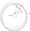 |
Fig. 1 Schematic representation of the belt orbits (solid gray and black) and the planet orbit (red) at the different stages of the ACE simulations: (a) the initial, circular, unperturbed belt; (a, b) the belt perturbed by the planet, but not modified by collisions; (b) the belt modified by collisions, but not by the perturber; (b, c) the belt modified by both the perturber and collisions. |
Assumed parameters for the parent belt.
2.3 Varied parameters
We varied a total of five physically motivated parameters in our study: the disk mass Mb, the belt widths, ∆ab, as well as the perturber mass, Mp, semimajor axis, ap, and eccentricity, ep. The parameter combinations assumed for belts and perturbers are summarized in Tables 1 and 2, respectively, together with the collisional settling time, tsettle, the initial perturbation time, tpre, and the period of full simulation of perturbations and collisions, tfull. We use the abbreviations given in the first columns of these tables to refer to individual model runs. For example, the run that combined the wider parent belt with an inner high-mass perturber is denoted w-i-M3, while the combination of a narrower belt with the low-eccentricity, high-mass inner perturber is denoted n-i-M3-le.
The effects of secular perturbation by a single perturber can be reduced to two main quantities: the timescale and the amplitude. To leading orders in orbital eccentricities and semimajor axes, the time required for a full precession cycle of grains launched from parent bodies on near-circular orbits at ab is given by (Sende & Löhne 2019)
 (1)
(1)
for perturbers distant from the belt, where M* = 1.92 M⊙ is the mass of the host star, Pb the orbital period of the parent bodies, and β the radiation-pressure-to-gravity ratio of the launched grains. Hence, the perturbation timescale is determined by a combination of perturber semimajor axis, perturber mass, and belt radius.
The amplitude of the perturbations is controlled by the forced orbital eccentricity that is induced by the perturber,
 (2)
(2)
around which the actual belt eccentricity evolves. This amplitude is determined by belt radius, perturber semimajor axis, and perturber eccentricity.
With the perturbation problem being only two-dimensional, we reduced the set of varied parameters by fixing the mean radius of the belt at 100 au, a typical value for cold debris disks observed in the far-infrared and at (sub)millimeter wavelengths (e.g., Eiroa et al. 2013; Pawellek et al. 2014; Holland et al. 2017; Sibthorpe et al. 2018; Matrà et al. 2018; Hughes et al. 2018; Marshall et al. 2021; Adam et al. 2021). For ab = const, which is a given parent belt, the timescale is constant for  and an inner perturber, or
  and an outer perturber. The amplitude is constant for
  and an inner perturber, or ep ∝ ap and an outer perturber. We expect degenerate behavior for some parameter combinations even in our reduced set.
The runs di, with an inner perturber closer to the belt, and o-M3, with an outer perturber, were constructed as degeneracy checks. Their outcomes should be as close to the reference run, n-i-M2, as possible. The perturbation timescales and amplitudes in the middles of the respective belts, given in Eqs. (1) and (2), are the same for all three parameter sets. For n-di the parameters listed in Tables 1 and 2 imply that differential precession acts on exactly the same timescale and with the same amplitude as in run n-i-M2 throughout the whole disk. The outcomes of the di runs, which had an inner perturber closer to the belt, should therefore be fully degenerate with the equivalent M2 runs. For the runs with an outer perturber, o-M3, the degeneracy applies only to the belt center because the sense of the differential perturbation is inverted as the exponent to ab changes from +7/2 to −3/2. The dependence on β is inverted too: the β-dependent term in Eq. (1) increases with increasing β for an inner perturber and decreases with increasing v for an outer perturber.
While Mp affects only the perturbation timescale, ap and ep affect the overall amplitude of the perturbations. In runs le we therefore lowered the perturber eccentricities to the more moderate value of ep = 0.3 (from the reference value, ep = 0.6). In an initially circular belt at 100 au, a perturber with ep = 0.3 at 20 au induces a maximum belt eccentricity that amounts to approximately twice the forced eccentricity given by Eq. (2), that is, ≈2 × 5/4 × 0.3 × 20/100 = 0.15 (compared to 0.30 for ep = 0.6). While planetary orbital eccentricities around 0.3 are common among long-period exoplanets, eccentricities around 0.6 are rare (Bryan et al. 2016). Likewise, belt eccentricities around 0.15 are closer to the maximum of what is derived for observed disks, as exemplified by the aforementioned disks around Fomalhaut, HD 202628, and HR 4796 A. Therefore, our reference case provides clearer insights into the expected qualitative behavior, while runs le are closer to observed disks.
The perturber determines the rate at which the secular perturbation occurs, while the collisional evolution in the belt determines the rate at which the small-grain halo is replenished and realigned. Collisions occur on a timescale given by the dynamical excitation, spatial density, and strength of the material. Instead of varying all these quantities, we varied only the disk mass (in runs m2 and m3) as a proxy for the spatial density. An increased disk mass and a reduced perturber mass are expected to yield similar results, as in both cases, the ratio between the timescales for collisional evolution and for secular perturbation is reduced. The total disk masses given in Table may seem low because the simulation runs are limited to object radii ≲0.5 km. However, when extrapolating to planetesimal radii ~100 km with a typical power-law index of −3.0…−2.8, as observed in the Solar System asteroid and Kuiper belts, the total masses increase by factors of (100/0.5)1.0…1.2 (i.e., by 2–2.5 orders of magnitude).
The belt width was varied explicitly in runs w. Not only do the belts in runs w have lower collision rates but also increased differential precession and potentially a clearer spatial separation of observable features.
Finally, we set up two runs that allow us to differentiate between the effects of the mean belt eccentricity, the differential precession of the belt, and the ongoing differential precession of the halo with respect to the belt. Only the last would be a sign of a currently present perturber. The first two could, for example, be the result of an earlier, ceased perturbation. In runs p0, we assumed belts with the same mean eccentricity and orientation as M2, but without any differential secular perturbation, that is, no twisted belt or halo. Such a configuration could result if the perturbations have ceased some time ago or the eccentricity was caused by another mechanism, such as a single giant breakup. In runs p1, the belts were initially twisted to the same degree as for n-i-M1 to n-i-M4, but no ongoing precession was assumed to drive the twisting of the halo. Ceased perturbation could be a physical motivation for that scenario as well. However, the main purpose of p0 and p1 was to help interpret the causes of and act as a baseline for features in the other simulation runs.
Parameter combinations for the perturbers.
2.4 Grain distributions for an inner perturber
Figure 2 shows distributions of normal geometrical optical thickness for grains of different sizes in run n-i -M2, our reference for subsequent comparisons. These maps resulted from a Monte-Carlo sampling of the q–e–ϖ phase space as well as mean anomaly. The maps show the contribution per size bin. The total optical thickness peaks at ≈3 × 10⁻⁵ in run n-i-M2, the total fractional luminosity at a similar value, which is a moderate value among the minority of mass-rich disks with brightness above current far-infrared detection limits (e.g., Eiroa et al. 2013; Sibthorpe et al. 2018) and a low value among those above millimeter detection limits (e.g., Matrà et al. 2018).
The big grains in Fig. 2d represent the parent belt, which started out circular and then completed almost half a counterclockwise precession cycle. The higher precession rate of the inner belt edge caused the left side to be diluted and the right side to be compressed, resulting in an azimuthal brightness asymmetry. This geometric effect of differential precession is notable only when the width of the belt is resolved. In wider belts, differential precession can create spiral density variations (Hahn 2003; Quillen et al. 2005; Wyatt 2005a). The effect becomes increasingly prominent over time or reaches a limit set by the belt’s self-gravity.
For smaller grains, the effects described in Löhne et al. (2017) come into play. Figure 2c shows the distribution of grains with radii s ≈ 9 µm. These grains are produced in or near the parent belt, but populate eccentric orbits as a result of their radiation pressure-to-gravity ratio β ≈ 0.23. Those grains born near the parent belt’s pericenter inherit more orbital energy and form a more extended halo on the opposite side, beyond the belt’s apocenter, in the lower part of the panel. At the same time, the alignment of their orbits creates an overdensity of mid-sized grains near the belt pericenter. The yet smaller grains in panels (a) and (b) tend to become unbound when launched from the parent belt’s pericenter, while those launched from the belt’s apocenter have their apocenters on the opposite side, forming a halo beyond the belt’s pericenter, in the upper parts of the panels. These effects are purely caused by the parent belt being eccentric.
The ongoing differential precession causes a misalignment of the halo with respect to the parent belt (Sende & Löhne 2019). This misalignment is more clearly seen in panels (b) and (c), which show a clockwise offset of the outer halo with respect to the belt, resulting from the wider halo orbits precessing at a lower rate. The population of halo grains is in an equilibrium between steady erosion and replenishment. Erosion is caused by collisions and PR drag, while replenishment is caused by collisions of somewhat bigger grains closer to the belt. The population of freshly produced small grains forms a halo that is aligned with the belt, while the older grains in the halo trail behind. The ratio of grain lifetime and differential precession timescale determines the strength of the misalignment. If the secular perturbation is strong or collisions are rare, the misalignment will be more pronounced, and vice versa. The smaller the grains, the higher are their β ratios, the wider their orbits, and the more they trail behind the belt.
A comparison of the most important timescales is given in Fig. 3. The collision timescale shown was obtained directly from ACE run n-i-M2, although it was very similar for all runs with the reference belt n. In runs with the wide belt w, the collision timescales were longer by a factor of two. In the more mass-rich belts m2 and m3 the collision timescales were correspondingly shorter. As a proxy to a PR timescale, Fig. 3 shows the e-folding time of the pericenter distances of grains with a size-dependent β ratio, launched from a circular belt of radius ab = 100 au (Sende & Löhne 2019):
![Mathematical equation: ${T_{{\rm{PR}}}} \equiv {q \over {\dot q}}\left( \beta \right) = 32\,{\rm{Myr}} \times {{1 - \beta } \over {\beta \left( {4 - 5\beta } \right){{\left[ {1 - 2\beta } \right]}^{1.5}}}}\left( {{{{a_{\rm{b}}}} \over {100\,{\rm{au}}}}} \right){{{M_ \odot }} \over {{M_*}}}.$](/articles/aa/full_html/2023/01/aa43240-22/aa43240-22-eq8.png) (3)
(3)
The PR timescale has a lower limit of 50 Myr, obtained for grains with β ≈ 0.2 (corresponding to radii s ≈ 10 µm), resulting in PR drag being insignificant in the presented model runs. A stronger contribution from PR drag would be expected for normal optical thickness ≲1 × 10⁻⁶ (Wyatt 2005b; Kennedy & Piette 2015), much less than the peak value of 3 × 10⁻⁵ reached in our disks. With collision timescale being proportional to disk mass squared and PR timescale being independent from disk mass, lowering the optical thickness (and hence the disk mass) by a factor of 30 would increase the collision timescale by a factor of ≈1000, bringing the green curve in Fig. 3 close to the black one for small grains. After simulations longer than the PR timescale, dust from the belt and halo could travel closer to the star, showing up in surface brightness maps at up to mid-infrared wavelengths, even for the optical thickness considered here (Löhne et al. 2012; Kennedy & Piette 2015; Löhne et al. 2017).
The time tfull is the time during which planetary perturbations and collisions were modeled simultaneously in our ACE runs. Over this period the complex belt eccentricity covered one sixth of a full precession cycle around the eccentricity that was forced by the perturber. Depending on the perturber-to-belt mass ratio, the collision timescale shown in Fig. 3 can be shorter or longer than the precession timescale for the grains that are most abundant and best observable, from the blowout limit at s ≈ 4 µm to s ≈ 1 mm. Where the collision timescale is shorter, the distribution can be considered equilibrated. Where the precession timescale is shorter, an equilibrium may only be reached after several full precession cycles, when the complex eccentricities are randomized. This long-term equilibrium after randomization is studied by Thebault et al. (2012), who find the resulting disks to be azimuthally symmetric. The numerical dispersion prevented us from following the evolution over such long timescales, which is why we limited this study to nonequilibrium, ongoing perturbation for the cases where precession timescales are shorter, that is, for the higher perturber-to-disk mass ratios. In runs n, grains with radii ≲20 µm have β ratios distributing them largely outside of the parent belt, forming the halo. Grains around that critical size have the shortest collisional lifetimes (see Fig. 3). For these grains differential precession and collisions do not reach an equilibrium if perturber-to-disk mass ratios exceed a factor of 100… 300, taking into account the extrapolation to largest planetesimal radii of ~ 100 km, as discussed in Sect. 2.3. When considering only the dust content, that is, grains up to roughly 1 mm in radius and Mb as given in Table 1, this mass ratio increases to 7000… 20 000. For grains with radii of 8 µm, where the halo extent is significant, the equilibrium is not reached when the perturber-to-disk mass ratio exceeds 10… 30 (or 700… 2000 for the dust content).
This leads to the question of how much of the halo asymmetry is actually caused by the already asymmetric belt. Figure 4 shows the distributions of bigger grains for runs (a) n-i-M2 and (b) n-p0. While n-i-M2 shows the features already discussed above, the belt in run n-p0 is purely eccentric, without the characteristic left-right asymmetry caused by differential precession. Run n-p1 is not shown, as it would be indistinguishable from n-i-M2. The corresponding distributions of smaller grains in runs n-i-M2, n-p0, and n-p1 are shown in panels (a), (c), and (e) of Fig. 5, respectively. As expected, the small-grain halo in run n-p0 shows no additional asymmetry. Run n-p1 has a belt that shows the same degree of asymmetry as that in run n-i-M2, but no ongoing precession that could further twist the halo. The slight misalignment of the small-grain halo in panel (e) is purely caused by the left–right asymmetry in density, and hence, collision rates in the parent belt. The n-p1 halo is already similar to the case of a low-mass perturber modeled in n-i-M1, shown in Fig. 6a, indicating that the effect of differential perturbations is weak compared to collisions in run n-i-M1. For the given combination of belt parameters and perturber orbit, the mass of a perturber able to twist the halo should exceed one Jupiter mass. This threshold is inversely proportional to the collisional timescale in the belt and directly proportional to the total dust mass.
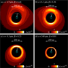 |
Fig. 2 Maps of contributions to face-on optical depth, τ, in run n-i-M2 from grains of four different size bins with mean grain radii s and corresponding β ratios, as labeled in the top-left corners of the panels. The orbits of the perturbers are shown with blue-green ellipses, and the host star is at the crossings of the major axes and latera recta. Dashed black-and-white ellipses trace the center of the parent belt. White lines show the orientations and lengths of the pericenters at the belt center (solid) and the belt edges (dashed). Arrows indicate the scale. |
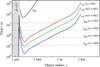 |
Fig. 3 Size dependence of timescales for collisions (solid blue, green, and red), PR drag (solid black), and a full secular precession cycle at 100 au (dashed black) for perturbers of different masses, as labeled. The timescales are calculated as described in Sende & Löhne (2019). |
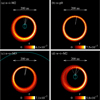 |
Fig. 4 Maps of contributions to face-on optical depth for grains of radius s = 5 mm in four different simulation runs: (a) n-i-M2, (b)n-p0, (c) n-o-M3, and (d) w-i-M2. See Fig. 2 for a detailed description. |
2.5 Dependence on parameters
Figure 6 shows the distributions of small grains for a series of runs with different perturber masses. The masses were increased by factors of five from run to run, and hence, the perturbation timescales decreased by factors of five. As a result, the misalignment of belt and halo increases monotonously from run n-i-M1 to run n-i-M4, as more and more halo grains from earlier stages of the precession cycle are still present. However, the misalignment is limited because the initial circular belt produced a radially symmetric halo that does not contribute to the azimuthal asymmetry.
The azimuthal distribution of small grains near the parent belt is another feature that is modulated by the strength of the perturbations. For a low-mass perturber that distribution is dominated by a combination of the overdensity near the belt pericenter and a remnant of the left-right asymmetry of the belt. For a high-mass perturber, where halos of a wider range of orientations overlap with old, symmetric halos, that pericenter overdensity is weakened with respect to the belt apocenter.
The azimuthally averaged size distribution depends only weakly on the degree of perturbation. Figure 7 shows small differences for grains between one and a few blowout radii among runs n-i-M1 through n-i-M4. These differences are caused mostly by the collisional lifetimes of grains near the blowout limit (as shown in Fig. 3) being longer than the total time over which the collisional cascade is simulated, tsettle + tfull. When translated to spatially unresolved spectral energy distributions, the resulting differences are small compared to uncertainties that arise from properties such as grain composition or dynamical excitation of the disk.
In a wider parent belt, the angular displacement between inner and outer edge is more pronounced, causing a stronger azimuthal asymmetry among the bigger grains in the parent belt. Figure 4d shows this distribution. In contrast, the resulting distribution of small grains (Fig. 5f), which is always more extended than the parent belt, does not differ much from the narrower belt in run n-i-M2 (Fig. 5a). While a yet wider belt can be expected to show differences in the small-grain halo, we refrained from performing additional simulation runs because such more diffuse belts would constitute a class of objects different from the narrow Fomalhaut-like belts we focus on. The results for the high-mass disks in runs m2 and m3 are not shown because they exhibit the expected similarity to n-i-M1, the run with the low-mass perturber. As anticipated in Sect. 2.3, the higher disk masses increase the collision rate, reducing the effect of the secular perturbations in the same way that the lower perturber mass does.
In runs le, the orbital eccentricities of the perturbers were halved. The resulting belt eccentricities follow suit, reducing the overall asymmetry of the belt and halo. The distribution of big and small grains is shown in Fig. 8. Compared to the n runs, the halos in the n-1e runs are more circular: wider near the pericenter of the belt and narrower near the belt’s apocenter (cf. Löhne et al. 2017). As a result, the semimajor axes and perturbation timescales of grains forming the halo on the apocenter side are shorter, closer to that of the belt. The resulting orientation of the halo follows that of the belt more closely than for a more eccentric perturber. The perturber mass threshold above which the twisted halo becomes notable is higher.
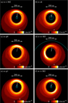 |
Fig. 5 Maps of contributions to face-on optical depth for grains of radius s = 7.5 µm in six different simulation runs: (a) n-i-M2, (b) n-di, (c) n-pβ, (d) n-o-M3, (e) n-p1, and (f) W-1-M2. See Fig. 2 for a detailed description. |
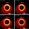 |
Fig. 6 Maps of contributions to face-on optical depth for grains of radius s = 7.5 µm in runs: (a) n-i-M1, (b) n-i-M2, (c) n-i-M3, and (d) n-i-M4. See Fig. 2 for a detailed description. |
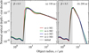 |
Fig. 7 Azimuthalfy averaged grain size distributions in terms of contribution to normal optical thickness at 100 au (left) and 200 au (right) for runs n-i-M1 (red), n-i-M2 (green), n-i-M3 (blue), and n-i-M4 (black). The dashed line traces the initial distribution common to all runs, with a lower radius limit at 100 µm. The gray-shaded region is dominated by grains on unbound orbits. |
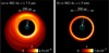 |
Fig. 8 Maps of contributions to face-on optical depth for grains of radii s = 7.5 µm (a) and s = 5 mm (b) in run n-M2-1e. |
2.6 Inner versus outer perturber
The expected degeneracy between runs with different inner perturbers is seen in Figs. 5a and b. Both runs, n-i-M2 and n-di, resulted in practically equal grain distributions because both perturbers exerted equal perturbations. Small differences could arise only from higher-order corrections to Eqs. (1) and (2). Such corrections were included for the involved semimajor axes but not for the eccentricities. Hence, the accuracy is limited for small grains on very eccentric orbits (see Sende & Löhne (2019) for a description of how orbits close to e = 1 are treated in ACE).
The o-M3 runs addressed the case of an outer perturber at 500 au that causes exactly the same perturbation of the belt center as the reference perturber i-M2, albeit at a perturber mass that is five times as high. Figures 4c and 5d show the resulting distributions of big and small grains, respectively. The outer perturber caused the outer belt edge to lead, the inner edge to trail, producing a big-grain asymmetry that is mirrored compared to the inner perturber. For actually observed disks and unobserved perturbers, these seemingly different cases can appear similar because the sense of the orbital motion in the disk, clockwise or counterclockwise, is usually unknown.
The distribution of smaller grains in n-o-M3 (Fig. 5d) differs from a pure mirror image of n-i-M2 (Fig. 5a). Instead of two azimuthal maxima, at the belt pericenter and apocenter, the outer perturber induced only one maximum, away from the apsidal line. This qualitative difference could be used to distinguish between an inner and an outer perturber. Another difference is the presence of small grains interior to the belt in run n-o-M3 (Fig. 5d). An outer perturber can, due to its proximity to the halo, further increase the orbital eccentricity of halo grains, shortening their periastron distances compared to the parent belt. The brightness maps shown by Thebault et al. (2012, their Fig. 10) exhibit a feature that is very similar, including the over-brightness on the periastron side. The contribution to this interior asymmetry from grains that are dragged in by the PR effect (cf. Löhne et al. 2017) is small in our case, but might be greater for the equilibrated disks discussed by Thebault et al. (2012). In our simulations, the distributions had an artificial cut-off at 40 au, the open inner edge of the pericenter grid described in Sect. 2.2. The observability of these features in and interior to the belt will be explored further in Sect. 4.3.
3 Observational appearance of sheared debris disks
Based on the spatial distributions of the dust discussed in Sect. 2, we investigated the imprint of planet-debris disk interaction for the considered scenarios on selected observable quantities. We assumed that the dust distributions are optically thin, that is, the observable flux density Sv results from the superposition of the individual contributions of the thermal emission and scattered stellar light of grains of all sizes. While – at a fixed radial distance to the star – the scattered radiation depends on the scattering cross section (Csca) and the Müller-matrix element S11, the emitted radiation depends on the absorption cross section (Cabs). For disks seen face-on, hence a fixed scattering angle, and assuming compact spherical grains all three quantities depend on the grain size, chemical composition, and observing wavelength. Therefore, multiwavelength observations potentially enable us to separate the contribution of certain grain sizes and allow us to conclude on the links between disk structure, dynamics, and eventually orbital parameters of an embedded exoplanet.
We present our method to compute brightness distributions from the spatial dust distributions computed with ACE and give a short discussion about the contribution of different grain sizes to the total flux in Sect. 3.1. Subsequently, in Sect. 3.2, we investigate the potential to observe the halo twisting discussed in Sects. 2.4–2.6. Any comments about the feasibility of observing our simulated distributions of surface brightness using real instruments are based on a performance analysis for a system at a stellar distance of 7.7 pc (e.g., Fomalhaut) that is presented in the appendix (see Appendix B). We focus our investigation on the systems with the parent belt of the reference parameter set n.
3.1 Brightness distributions
To compute surface brightness maps, we extended the numerical tool Debris disks around Main-sequence Stars (DMS; Kim et al. 2018) by an interface to process the spatial grain distributions computed by ACE. In DMS, an optically thin dust distribution is assumed to compute maps of thermal emission and scattered stellar light. Host star and optical grain properties are modeled likewise as described in Sect. 2.2.
To establish a vertical structure from the two-dimensional spatial grain distributions, we assume a wedge-like structure of the debris disk with a half-opening angle of 5° and a constant vertical grain number density distribution. Furthermore, we considered disks in face-on orientation. Therefore, the possible scattering angles are all close to 90° where the Müller-matrix element S 11, describing the scattering distribution function, shows a smooth behavior. Nonetheless, the perfect homogeneous spheres as they are assumed in Mie theory are only a coarse approximation, especially for large grains (e.g., Min et al. 2010).
With ACE we simulated the evolution of bodies with radii up to 481 m. However, grains with sizes much larger than the observing wavelength hardly contribute to the total flux. For this reason, we neglected large grains in the computation of brightness distributions by applying the following criterion: If grains of the next larger size bin would increase the total flux of the reference system with parent belt n and inner perturber i-M2 (n-i-M2) at an observing wavelength of 1300 µm by less than 1 %, neglect these and even larger grains. Using this criterion, we included grains with radii of up to 5.65 cm. For the system n-i-M2, the dust mass up to that grain size is ≈1.1 × 10⁻⁸M⊙; up to the grain size of ≈1 mm it is ≈2.7 × 10⁻⁹ M⊙. The latter value fits well into the range of dust masses of cold debris disks around A-type stars derived by Morales et al. (2013, 2016) who found values between ≈5.5 × 10⁻¹⁰ and 4.8 × 10⁻⁸ M⊙. The systems with the reference belt n combined with other perturbers possess slightly different dust masses due to a different amount of grain removal and period of simulation tfull; the deviations compared to system n-i-M2 are smaller than ± 10 %.
We chose five observing wavelengths motivated by real astronomical instruments that allow us to trace grains of sizes ranging from several micrometers to several hundreds of micrometers. Neglecting the contribution of the central star, in the K band (2 µm) the flux is entirely dominated by the stellar light that has been scattered off small dust grains. Likewise, this is the case in the N band (10 µm) but with a small contribution (≲10 %) of thermal emission of small dust grains. In the Q band (21 µm) and at a wavelength of 70 µm we trace the thermal emission of small halo grains, while at a wavelength of 1300 µm we trace the thermal emission of the largest and coldest grains, which indicate the position of the parent belt. At wavelengths of 2 µm, 10 µm, and 21 µm we will see major improvements regarding angular resolving power and sensitivity of imaging instruments due to the Multi-Adaptive Optics Imaging Camera for Deep Observations (MICADO, Davies et al. 2018, 2021) and the Mid-Infrared ELT Imager and Spectrograph (METIS, Brandl et al. 2014, 2021) at the Extremely Large Telescope (ELT)1 as well as the Near-Infrared Camera (NIRCam, Horner & Rieke 2004) and the Mid-Infrared Instrument (MIRI, Wright et al. 2004) on the James Webb Space Telescope (JWST, Gardner et al. 2006). In Table 3, the selected observing wavelengths, the type of radiation dominating the flux at those wavelengths, and corresponding exemplary instruments with high angular resolving power are listed.
In Fig. 9, the central ~ 190 au of the brightness distributions at all five wavelengths for the system n-i-M2 (top row) and the system with the reference parent belt n and the o-M3 perturber orbiting outside thereof (n-o-M3; bottom row) are displayed for illustration. These particular systems have been chosen because the perturbation timescales and amplitudes of their belt centers are equal (see Sect. 2.6). Thus, from any possible pair of systems with an inner and an outer perturber, the effect on the spatial dust distribution by the parent belt being eccentric is most similar. The differences are apparent due to the perturber orbiting inside (n-i-M2) or outside (n-o-M3) the parent belt. For illustrative reason, the brightness distributions were normalized to the maximum flux density Sv, max of each map at the respective wavelength. The un-normalized distributions are shown in the Appendix (see Fig. B.1).
All systems with an inner perturber show comparable brightness distributions. Taking the system n-i-M2 as an example, we find the brightness distributions to be similar at the wavelength pairs {2 µm, 21 µm} and {10 µm, 70 µm}. At the former two wavelengths, the ring-like structure is broader and the relative contribution from outer regions ≳ 100 au is stronger than at the latter two. The map at 1300 µm differs from the maps at 10µm and 70µm only by the dimmer emission in the outer regions. This findings can be explained by the contribution of grains near the blowout limit of sbo ≈ 4 µm. For illustration, azimuthally averaged radial brightness profiles for the system n-i-M2 (see the upper row in Fig. 9) as well as the relative contribution of two different grain size groups are shown in Fig. 10. While the distributions of grains near the blowout limit can be oriented opposite to the parent belt, the distribution of larger grains share the orientation of the belt (see Fig. 2a in contrast to 2b). At the wavelength pair {2 µm 21 µm} the radiation of the smallest grains makes up a large part of the total emission at large separations from the host star ≳ 100 au while in the wavelength pair {10 µm, 70 µm} this is not the case. The smallest grains scatter the stellar radiation very efficiently at 2 µm while their relative contribution drops toward larger wavelengths. At a wavelength of 10 µm, scattering by larger grains dominates the net flux. At a wavelength of 21 µm, which is dominated by thermal dust emission, the smallest grains are the most efficient emitters due to their highest temperature. The relative contribution of the smallest grains becomes less important at 70 µm and even negligible at 1300 µm. At the latter wavelength, only the emission of the largest grains close to the parent belt is visible.
For the systems with an outer perturber and taking the system n-o-M3 as an example, we see that the overall appearance at different wavelengths is very similar to the one at 1300 µm, while toward shorter wavelengths the relative contribution from outer regions ≳ 100 au increases due to the growing contribution of smaller grains on extended orbits. This behavior is constant for the other systems with different perturber parameters. Furthermore, we see emission from regions inward of the belt location, most pronounced at 10 µm and less pronounced at 2 µm, 21 µm and 70 µm. This flux stems from small grains that are forced by the perturber on orbits leading into that inner disk region. The location and intensity of those features in the brightness distributions are individual for each system and depend on parameters of the perturber (see also Sect. 4.2).
Considered observing wavelengths.
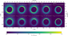 |
Fig. 9 Surface brightness distributions of the system with parent belt n and perturber i-M2 orbiting inside the belt (n-i-M2; top row) and the system with belt n and perturber o-M3 orbiting outside the belt (n-o-M3; bottom row) for a stellar distance of 7.7 pc at five wavelengths: 2 µm, 10 µm, 21 µm, 70 µm, and 1300 µm (from left to right), zoomed in on the central ~190 au. Each distribution has been normalized by its respective maximum value, Sv,max. The white asterisk denotes the position of the central star and defines the center of the coordinate system. |
3.2 Twisting of the small grain halo
To analyze the small grain halo, we fitted ellipses to lines of constant brightness (isophotes) radially outside the parent belt. First, we produced polar grids of the Cartesian flux maps using the Python package CartToPolarDetector2 (Krieger & Wolf 2022): after superposing the Cartesian grid with the new polar one, the polar grid cells were computed by summing up the values of the intersecting Cartesian cells, each weighted with its relative intersecting area with the new polar cell3. The new polar coordinates are the distance to the center, r, and the azimuthal angle, θ, which is defined such that 0° is oriented in the direction of the horizontal axis toward the west (i.e., right) side of the map and the angle is increasing counterclockwise.
Second, we determined the polar coordinates of selected brightness levels. To trace the halo around the parent belt, we required all isophotes to be radially outward of the parent belt. To achieve this, we first defined a reference brightness value for each map representing the mean flux level of the bright ring: We determined the radial maxima of brightness for each azimuthal angle θ and derived the reference value as the azimuthal average of the radial maxima. Taking this reference value, we acquired a reference isophote. Lastly, we computed ten isophotes that are radially outward of the reference isophote for all azimuthal angles and with a brightness level of at most 80 % of the reference value. As a lower cutoff, we set 1 % of the reference value.
Assuming the central star to be in one of the focal points and the respective focal point to be the coordinate center, we used the ellipse equation
 (4)
(4)
with the azimuthal angle θ and the parameters semimajor axis a, eccentricity e, and the position angle of the periapse ϕ, where ϕ corresponds to the longitude of periapse ϖ for the face-on disks discussed here4. For illustration, the polar brightness map of the system n-i-M2 with indicated brightness levels and fitted isophotes is shown in Fig. 11a. By comparing the orientation of isophote ellipses for different semimajor axes, we can analyze whether the rotation of the small grain halo with respect to the parent belt, as presented in Sect. 2.5, can be quantified by analyzing maps of surface brightness.
Figure 12 shows the results of ellipse orientation relative to the orientation of the innermost ellipse ∆ϕ for the wavelengths of 2 µm, 10 µm, 21 µm, and 70 µm. At these wavelengths we trace small grains that form an extended halo (see Fig. 2). Likewise, as discussed in Sect. 3.1, all results for systems with an inner perturber show a similar behavior at a fixed respective wavelengths. Furthermore, for a fixed system the maps at wavelength pairs {2 µm, 21 µm} and {10 µm, 70 µm} show similar trends, respectively.
At the wavelength pair {2 µm, 21 µm}, we see that isophotes with small semimajor axes a show a small, but monotonous change in orientation with increasing values of a. This is caused by theongoing differential precession(see Sect. 2.5 and Sende & Löhne 2019). Grains populating regions with increasing distance from the center, marked by isophotes with largersemimajoraxes, are increasingly older and therefore trail the farther precessing parent belt, marked by isophotes with smaller semimajor axes, more. Then, this trend is followed by a flip of ∆ϕ ~ − 180° over a small interval of a. The flip appears, because at these two wavelengths and large semimajor axes the brightness contribution of the smallest, barely bound grains near the blowout limit of sbo ≈ 4 µm starts to dominate (see Fig. 10). These grains form a halo inversely oriented to the parent belt (see Fig. 2a and Sect. 3.1). At 2 µm the flip starts at a ~ 170 au and ends at a ~ 250 au. At 21 µm it starts at semimajor axes of a ~ 170 au but is completed sooner at a ~ 210 au–220 au. The different location of the flip between the two observing wavelengths is caused by the varying fraction of the contribution of the smallest grains to the total brightness at different separations from the star: at a wavelength of 21 µm, the emission of the small grains dominates over those of larger grains already at smaller separations from the central star than at 2 µm (compare the first and third panel of Fig. 10). Lastly, for further increasing semimajor axis a the flip is followed by decreasing values of ∆ϕ. This is again caused by the ongoing differential precession.
At the wavelength pair {10 µm, 70 µm} we do not find this behavior. Instead, because the brightness contribution of the smallest grains causing the flip is much weaker at these wavelengths, we find a mostly monotonous decrease in isophote orientation ∆ϕ with increasing semimajor axis a, explained by differential precession.
At the wavelength pair {10 µm, 70 µm} and for separations from the host star ≲200 au also at 2 µm, variations in the relative isophote orientation ∆ϕ are correlated with the perturber mass: the lowest mass perturber i-M1 causes the smallest, the highest mass perturber i-M4 the largest values of ∆ϕ. This is related to the angular velocity of the differential precession. The higher the perturber mass, the faster the parent belt precesses, causing the small grain halo to lag behind more.
At the wavelength pair {2 µm, 21 µm} we see exactly the opposite separation by perturber mass: In the system with the i-M1 perturber the isophote orientation flips at the smallest semimajor axes and within the smallest axes interval, while in the system with the i-M4 perturber it does so at the largest semimajor axes and within the broadest axes interval. This behavior is directly related to the semimajor axes distribution of the grain orbits. For a certain grain size, the more massive the perturber is, the larger is the inner gap of the entire debris disk and the halo of small grains. As the location where the flip occurs is determined by the radial distance where the brightness contribution of grains near the blowout limit starts to dominate, a system with a more massive perturber shows the flip in isophote orientation ∆ϕ at larger values of the semimajor axis a than a system with a less massive perturber.
Contrary to the analysis of systems with an inner perturber, no clear trend is found for systems with an outer perturber. For the systems n-o-M2 and n-o-M3, we find isophotes strongly different than those of n-o-M4. The first two systems show only small isophote rotations over all semimajor axes a in the maps at the wavelengths 2 µm, 10 µm, and 70 µm. At 21 µm n-o-M2, n-o-M3 show a clockwise isophote rotation of up to ∆ϕ ~ 10°, 20° for small semimajor axes that turns into a counterclockwise rotation of up to ∆ϕ ~ − 80° for semimajor axes of a > 130 au, 140 au, respectively. The isophote rotation of the n-o-M4 perturber maps show a consistent behavior at all wavelengths from 2 µm to 70 µm: for small semimajor axes we see only small values of ∆ϕ. At semimajor axes of a ~ 170 au–190 au the isophotes rotate clockwise up to ∆ϕ ~ 100°–120°. The nonuniform behavior of the isophote orientation ∆ϕ derived from the maps of systems with an outer perturber results from the fact that each outer perturber system shows highly individual spatial distributions for small grains. Furthermore, while for the systems with an inner perturber the spatial dust distributions change only slowly with grain size (see Figs. 2b and c), for the systems with outer perturbers they vary strongly in shape and density with grain size. As a consequence, the isophotes deviate more from an elliptical shape and do not possess a common orientation. To illustrate this behavior, the polar brightness map of the system n-o-M4 with indicated flux levels and fitted isophotes thereto is shown in Fig. 11b.
The small grain halo is a rather faint part of a debris disk system. Within our framework, most promising to detect and constrain it are observations at a wavelength of 21 µm using JWST/MIRI. With an exposure time of 1 h, the differential rotation manifested in the monotonous change of isophote orientation for small semimajor axes up to a ~ 140 au – 160 au can be detected. With an exposure time of 5 h, surface brightness levels corresponding to isophotes with semimajor axes of a ~ 190 au–220 au can be detected, covering almost the entire flip of isophote rotation. Furthermore, observing with the Photodetector Array Camera and Spectrometer (PACS, Poglitsch et al. 2010) on the Herschel Space Observatory (Pilbratt et al. 2010) at the wavelength 70 µm for an exposure time of 1 h would have been sufficient to detect parts of the halo corresponding to isophotes with semimajor axes of up to a ~ 220 au–240 au. More details on the observational analysis are provided in Appendices B and B.1.
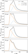 |
Fig. 10 Radial brightness profiles normalized by their respective maximum value, Sv,rp,max, at the wavelengths 2 µm, 10 µm, 21 µm, and 70 µm of the system with the reference planetesimal belt n and the i-M2 inner perturber (n-i-M2). The dotted blue line shows the relative contribution of radiation from grains with radii s ≤ 4.9 µm, the dashed orange line of grains with radii s ≥ 6.1 µm, and the solid black line shows the total emission as the sum of the two fractions. The radial profiles of each wavelength are normalized to the maximum value of the respective total brightness profile. |
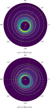 |
Fig. 11 Polar brightness maps of the systems n-i-M2 (same as in Fig. B.1a) and n-o-M4 at a wavelength of 2 µm (radius 400 au). The white asterisk denotes the position of the central star and defines the center of the coordinate system. The white crosses trace five lines of constant brightness (isophotes) and are drawn every 7.5°. The colored ellipses have been fitted to the respective isophotes using Eq. (4) with the central star in one of the focal points. The dashed lines give the direction from the focal point to the periapse, that is, ϕ + π, and are drawn in the same color as their corresponding ellipse. |
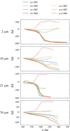 |
Fig. 12 Orientation, ∆ϕ, of the isophote ellipses relative to the orientation of the innermost ellipse drawn over semimajor axis a. A negative value of ∆ϕ means clockwise rotation and a positive value counterclockwise rotation. Solid lines are used for the systems with inner perturbers and dashed lines for those with outer perturbers, and rows are used to show four different wavelengths tracing small halo grains: 2 µm, 10 µm, 21 µm, and 70 µm. |
4 Feasibility of distinguishing between the existence of an inner or outer perturber
Motivated by the notably different distributions of small grains in systems with an inner and outer perturber, respectively (Sect. 2.6), and their corresponding brightness distributions (Sect. 3.1), we investigated the feasibility of distinguishing between those two types observationally. We identify several disk properties and features that can be used to accomplish this task (Sects. 4.1–4.3). The presentation of each feature is paired with an explanation of its origin by discussing the underlying spatial dust distributions and an estimation of the feasibility of observing it based on the analysis in Appendix B. While restricting the detailed discussion on systems with belts simulated with the reference parameter set n, we comment on other systems simulated with the other sets w, m2, and m3 in Sect. 4.4. In Sect. 4.5, we summarize the analyses to a simple flowchart, allowing one to decide whether a debris disk harbors a single inner or outer perturbing planet.
4.1 Spiral structure in the Q band
We find that a spiral structure is solely produced by inner perturbers, best visible in the Q band at 21 µm (for an illustration, see Fig. 13). The location of the structure is completely consistent with the location of the parent belt (contrary to the systems with an outer perturber as discussed in Sect. 4.2), which we trace by isophotes of 1 % of the maximum brightness in the corresponding 1300 µm map.
The spiral structure originates in the superposed brightness contribution of several grain sizes with different spatial distributions. We exemplify this in detail using Fig. 13: at the northeast of the map5 and moving clockwise, the brightness distribution forming the inner spiral arm is dominated by the thermal radiation of grains of size s ≳ 240µm until the southwest of the map, while the brightness distribution forming the remaining spiral arm in clockwise direction is dominated by the radiation of grains s ~ 5 µm in size (see Fig. 2a and Fig. 2d for similar distributions of the system n-i-M2). In the brightness distributions of the systems with the lower mass perturbers (i-M1 to i-M3) we find the same spiral structure. However, its contrast is lower in these maps but decreases not monotonically with the perturber mass. This is because the respective systems show similar – but slightly shifted – spatial dust distributions compared to n-i-M4. Their distributions overlap more strongly, and therefore, the spiral structures in these maps are less rich in contrast. This example illustrates that the specific contrast of the spiral structure depends on the individual system. The systems with an outer perturber do not show that spiral patterns because the grains of the respective sizes have different spatial distributions.
We see strong emission from the s ~ 5 µm sized grains at a wavelength of 2 µm (see Sect. 3.1) as well. However, at that wavelength other similarly sized grains with slightly different spatial distributions contribute considerably to the net flux, effectively smearing out the spiral structure. In the brightness distributions at the wavelengths 10 µm and 70 µm, which are not sensitive to emission of s ~ 5 µm sized grains (see Sect. 3.1), the spiral structure is not visible at all. While at 2 µm the contrast of the structure is not sufficient, and at 10 µm and 70 µm it does not appear, a wavelength of 21 µm is suitable to observe such structures with JWST/MIRI: With an exposure time of 8 h it is possible to achieve the required contrast to detect the spiral pattern for the system n-i-M4 (see Appendices B and B.2).
4.2 Grains scattered inward of the parent planetesimal belt
To analyze the disk regions in the maps inward of the parent belt, we defined this inner disk region to be inward of the isophote with a brightness value of 1 % of the maximum brightness in the corresponding 1300 µm map. For the systems with an inner perturber, we find that the brightness decreases quickly inward of the parent belt to levels several orders of magnitude lower than the average, regardless of wavelength (see the top row in Figs. 9 and 13). However, this is not the case for the systems with an outer perturber. At the wavelength of 2 µm, 10 µm, 21 µm, and weakly at 70 µm, there is an considerable amount of light coming from the inner disk region. Depending on observing wavelength and perturber parameters it reaches levels of up to several tens of the maximum brightness values (for an illustration, see Fig. 14). We note that the sharp cut-off at a distance of 40 au is an artifact caused by the inner edge of the pericenter grid in the ACE simulations. At 10 µm, while the brightness from the belt location and outer regions is dominated by scattered stellar light, the brightness from those inner regions is dominated by thermal emission.
This flux originates from grains of the size s ~ 3 – 12 µm. The outer perturber orbits near the small grain halo and forces grains on orbits leading inside the parent belt. Although the exact spatial grain distributions and thus the characteristics of the brightness distribution inside the parent belt strongly depend on the exact perturber parameters, we find brightness levels up to several fractions of the maximum brightness at the region inward of the parent belt for all investigated systems with an outer perturber but for none of those with an inner perturber. We note that the smallest bound grains populate orbits that cross or nearly cross the orbit of the outer perturber. Hence, the model accuracy is lowest for these grains and the scope of a quantitative analysis limited.
However, the lack of such emission from regions inside the parent belt is not a viable criterion for the presence of an inner perturber because in our model setup the inner regions are clear from emission regardless of the presence of an inner perturber.
While at the wavelength of 10 µm exposure times of ≳ 10 h are required when observing with JWST/MIRI, at the wavelength of 21 µm an exposure time of 1 h is sufficient to detect the emission from inside the parent belt with the aforementioned caveat of limited accuracy for grains that orbit close to the perturber (see Appendices B and B.3).
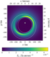 |
Fig. 13 Surface brightness distribution for a stellar distance of 7.7 pc at the wavelength 21 µm (Q band) of the system with belt parameter set n and the inner perturber i-M4 (n-i-M4). The contour lines denote the isophotes of the corresponding 1300 µm map of the same system with a flux density level of 1 % of its maximum value. They enclose the position of the parent planetesimal belt. General figure characteristics are the same as in Fig. 9. |
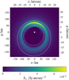 |
Fig. 14 Surface brightness distribution for a stellar distance of 7.7 pc at the wavelength 10 µm (N band) of the system with belt parameter set n and the outer perturber o-M3 (n-o-M3). General figure characteristics are the same as in Fig. 9, and white contour lines have the same meaning as in Fig. 13. |
4.3 Number of azimuthal radial flux maxima
As mentioned in Sect. 2.6, the system n-o-M3 with an outer perturber shows one azimuthal maximum in the distribution of small halo grains while the system n-i-M2 with an inner perturber shows two (for an illustration, see Figs. 5d and 5a). Likewise, we find this to be the case for the systems with perturbers of different masses as well. In the following we investigate whether this feature appears in the brightness distributions by analyzing the bright ellipsoidal structure. In Fig. 15, the radial maxima, as computed in Sect. 3.2, over the azimuthal angle θ are displayed, separated for systems with an inner and with an outer perturber.
First, we discuss the systems with an inner perturber: at a wavelength of 1300 µm, we find one global maximum and one minimum at angles of θ ~ 60° and 200°, respectively. At the wavelengths 2 µm, 10 µm, and 21 µm, the first maximum at around θ ~ 20°–60° is congruent with the maximum at 1300 µm, the second is located at θ ~ 240°. While the second maximum is very pronounced at 2 µm and 21 µm, at 10 µm it appears less pronounced. At 70 µm, it is only visible as a small shoulder on the increasing flank of the global maximum for all systems except n-i-M1. The system n-i-M1 generally represents an exception: At the wavelength of 2 µm the second maximum is misplaced compared to the other systems and located at θ ~ 260° and it shows another smaller local maximum at θ ~ 320°; at 21 µm, there are several small local maxima located around θ ~ 190°–320°; at 10 µm there is no second maximum. The system n-i-M1, whose perturber has the lowest mass, represents an intermediate step between the stronger perturbations in the systems with perturber i-M2, i-M3, i-M4 and the ceased perturbations in system n-p1. To illustrate this, the system n-p1 is added to the inner perturbers as a reference in Fig. 15.
The first maximum around θ ~ 20°–60° is produced by the superposed contributions of various grain sizes s ≳ 15 µm. Therefore, that maximum appears over a large wavelength range. As the grain distributions vary slightly between systems with different perturbers and the relative contribution of the individual grain sizes on the net flux varies with wavelength, the azimuthal position of the radial maximum changes slightly with perturber parameters and wavelength. The second maximum at θ ~ 240° originates from ~5 µm grains. As shown in 3.1, these grains contribute a large fraction of the net flux at the wavelengths of 2 µm and 21 µm, but not at 10 µm and 70 µm. This is the reason for the smaller height of the second maximum at 10 µm and its absence at 70 µm.
For the systems with an outer perturber we find no second maximum and only one global maximum and minimum, respectively, regardless of wavelength. In contrast to systems with an inner perturber, the systems with an outer perturber do not show a prominent spatial overdensity of ~5 µm grains able to produce a pronounced second maximum. The only exception is the system n-o-M2, where a less pronounced second maximum is located at θ ~ 280°. Furthermore, run n-o-M2 shows a minor deviation from the general trend at 10 µm, a small additional local maximum is located at θ ~ 50°. The global maximum is located at around θ ~ 80°–110° for the systems with perturbers n-o-M1 to n-o-M3. The system with the highest mass perturber n-o-M4 shows a slightly deviating position.
Concluding, by using the azimuthal location of the maximum of radial flux density, we identified two ways of distinguishing between systems with an inner versus those with an outer perturber. First, if we find two azimuthal maxima at the wavelengths 10 µm or 21 µm, an inner perturber is indicated. As inner perturbers with low masses may produce obscure second maxima (such as the system n-i-M1) or the maxima might be undetectable because of observational limitations, the absence of such a second maximum is a necessary, but not sufficient criterion for an outer perturber system. At 2 µm, a clear differentiation is not possible, as a second maximum, much smaller than the global, can also be produced by systems with an outer perturber. Nonetheless, if that second maximum at 2 µm is accompanied by second maxima at larger wavelengths, an inner perturber is indicated.
A second way to distinguish between the two types of systems is to measure relative location of a maximum and minimum of the contrast ≈ 1.7 (2.2) for inner (outer) perturber systems at the wavelength of 1300 µm. For the systems with an inner perturber, the angular distance between these extrema is ∆ϕmin-max ≈ 140° while the systems with an outer perturber appear symmetric with ∆ϕmin-max ≈ 180°. Within our investigated parameter space, this behavior is independent of perturber mass. The relative location of the maxima at 1300 µm depends on which parts of the parent belt lead and trail during precision. For the systems with an inner perturber the inner edge of the belt leads while the outer trails and vice versa for systems with an outer perturber (see Sect. 2.6).
We estimated the exposure time required to achieve a sufficient contrast for distinguishing the second local maximum at θ ~ 240° from its consecutive minimum for the system n-i-M2 when observing with JWST/MIRI at 21 µm and found 1 h to be sufficient (see Appendices B and B.4). Furthermore, we compiled the flux contrasts between the different azimuthal maxima and minima in Table 4. For disks with an outer perturber, the contrast is notably higher, in particular at mid- and far-infrared wavelengths. This is a direct consequence of the lack of a second local brightness maximum.
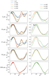 |
Fig. 15 Azimuthal distribution of radial maxima of brightness normalized by their respective maximum value, Sv,max, in the five investigated wavelengths: 2 µm, 10 µm, 21 µm, 70 µm, and 1300 µm. Left: Systems with an inner perturber. System n-p1 is displayed as a reference that shows the case without ongoing precession. Right: Systems with an outer perturber. |
4.4 Other parent planetesimal belts
To investigate the impact of the parent belt parameters on the observational appearance of the debris disk system, we analyzed brightness distributions of the systems with the parameter sets of the parent belt w, m2, and m3 combined with the parameter set of the inner perturber i-M2 and the outer perturber o-M3 and compared them to the results of the systems simulated with the reference belt parameter set n, that is, n-i-M2 and n-o-M3.
In the brightness distributions of the inner perturber systems with the different belt parameter sets, we can find the same halo twisting as for the system n-i-M2. Furthermore, we see the expected difference in the level of twisting: the system with parameter set w-i-M2, which possesses the longest collision timescale, shows the most trailing halo while the system with parameter set m3-i-M2, which possesses the shortest collision timescale, shows the least trailing halo (see Sect. 2.2).
Regarding the disk characteristics used to differentiate between systems with an inner or an outer perturber, the systems with parent belt parameter sets w, m2, and m3 show no major differences compared to those with set n. The system with parameter set w-i-M2 shows an increased contrast of the spiral structure in the Q band compared to n-i-M2 due to the spatially more extended emission. All systems with an outer perturber show nonzero brightness in the region inward of the parent belt. However, a variation in the belt parameters causes its shape and position to vary, similar to a variation of the perturber parameters.
Concerning the second azimuthal maximum at around θ ~ 240° (see Sect. 4.3) for systems with an inner perturber: As predicted in Sect. 2.3, the system with belt parameter set w shows an increased contrast of that second maximum. Furthermore, we find an increased contrast between maximum and minimum at a wavelength of 1300 µm. The broader parent belt of the system causes the dust distribution at the belt apocenter to be more diluted, increasing the contrast of the extrema.
To the contrary, the belts with parameter sets m2 and m3 show a smaller second maximum. The higher belt mass decreases the collisional timescale, which causes small grains to be replenished more quickly, in turn decreasing the relative contribution of older small grains on more extended orbits to the net flux. Furthermore, we see the predicted degeneracy between a system with a low mass perturber and a system with a high mass parent belt: the brightness distributions of the systems with parameter sets n-i-M1 and m3-i-M2 appear similarly. For systems with an outer perturber, a variation of the parent belt parameters causes almost no change in the azimuthal trend of radial maxima. However, we identify two minor effects: the parent belt with parameter set w causes an higher contrast between maximum and minimum at a wavelength of 1300 µm, similar to the system with an inner perturber (w-i-M2). Furthermore, the system with parameter set m3-o-M3 shows a small secondary maximum at a wavelength of 2 µm, similar to that of the system with set n-o-M2, which is again an expression of the degeneracy of perturber and parent belt mass. At a wavelength of 1300 µm we find no difference in the azimuthal trend of radial maxima for varying parent belt mass; the systems with the belt parameter sets n, m2, and m3 appear the same.
Flux contrast of azimuthal flux maximum to minimum.
4.5 Flowchart for distinguishing between inner and outer perturbers
We compile the results of the analysis presented in Sects. 4.1–4.3 in a decision flowchart, displayed in Fig. 16. For this flowchart we assumed that exactly one (dominant) inner or outer perturber orbits the system.
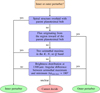 |
Fig. 16 Flowchart for deciding whether an inner or outer perturber orbits in the system based on distinct observable features of a debris disk system. |
5 Discussion
5.1 Numerical dispersion
We could show that a grid-based model of a collisional cascade can be combined with a TVD advection scheme for PR drag and secular dynamical perturbations. The upwind scheme used in previous ACE versions is suitable for scenarios were a stream of small particles springs from a continuous supply in a static belt of bigger objects. The population of small grains decays collisionally, for example during PR-induced drift toward the star, resulting in smooth distribution. The distribution of bigger source objects is confined more sharply, but does not migrate. In the case of the secular perturbations discussed here, that static picture no longer applies. When dynamical perturbations move the source region itself through the phase space, the belt’s sharp features will be dispersed over time, artificially broadening narrow disks or exciting dynamically cold disks. After some time, the simulation results do no longer reflect the intended physical scenario (Sende & Löhne 2019). We addressed this problem with the introduction of a second-order TVD scheme to the ACE code, reducing the dispersion. While dispersion is still significant, integration is now possible over a longer period of time (see Appendix A for more details).
Further improvements could include a return to a semimajor axis grid instead of the current pericenter grid. That step would eliminate the dispersion in one dimension because secular perturbations do not affect the semimajor axes. The pericenters are affected because they depend on eccentricity: q = a(1 − e). On the other hand, a pericenter-based grid can represent the orbits of halo grains on highly eccentric orbits more accurately, preserving their origin in the parent belt and their collision rates and velocities there. For the problem at hand, where both the halo of small grains and the parent belt are important, none of the two options provides a clear advantage.
The angular dispersion in ϖ could be reduced further by a “co-precessing” grid that follows the parent belt’s orientation. A mean precession  , weighted by the masses in individual bins, could be calculated for each time step and then subtracted. The advection through the grid would be reduced to differential precession relative to the mean belt. We will implement and test this modification in future work.
A consequent iteration on a grid that follows the mean precession would be a grid where the individual bins completely follow the advection stream. Instead of moving material from bin to bin, the bins themselves would move. No dispersal could occur. However, the current rigid discretization with separate grids for m, q, e, and ϖ allows for optimizations that make use of an azimuthal symmetry in the collision physics, even if the material distribution itself is not azimuthally symmetric. Variable, asymmetric discretization would increase computational costs of the collisional cascade model drastically, necessitating a reduction in grid resolution. The non-static bins in such an approach would be similar to the so-called tracers used in the LIPAD code (Levison et al. 2012). The superparticles adopted in LIDT-DD (Kral et al. 2013) and SMACK (Nesvold et al. 2013) differ more strongly because the particle ensembles are not orbit-averaged there. The same applies to the destruction-only approach called collisional grooming, which is used by Stark & Kuchner (2009) and in the DyCoSS code (Thébault 2012; Thebault et al. 2012).
5.2 Scope of the perturbation scenario
We modeled debris disks that are secularly perturbed by a single companion on an eccentric orbit distant from the planetesimal parent belt. The induced differential precession leads to asymmetries in belt and halo that are reflected in scattered light and thermal emission maps. The considered perturber masses are high, ranging from half a Jupiter mass to roughly 0.06 solar masses. The models are not applicable to Neptune or Earth-mass planets. Firstly, perturber masses should match or exceed disk masses in order to perturb with a significant amplitude. The dust-rich debris disks that are most easily detected are expected to be collisionally replenished from massive planetesimal belts, possibly totaling hundreds of Earth masses (Thébault et al. 2006; Krivov et al. 2018), assuming biggest planetesimals with diameters on the order of ~100 km. Even minimum total disk masses, assuming at most km-sized objects, reach tens of Earth masses (Krivov & Wyatt 2021).
Secondly, the described effects of differential precession require the perturber to overcome the self-gravity of the disk. The precession induced in the halo by the planetesimal belt will drag the halo along with the belt, reducing the differential precession and the trailing of the halo caused by an inner perturber.
Both timescale and amplitude of the perturbations favor the planetesimal belt over the planetary perturber because the belt is closer to the outer halo than an inner planet. When belt and perturber are of similar mass, the belt will dominate the halo’s dynamical evolution because of its proximity. The further away from the belt the inner perturber is, the greater must be its mass in excess of the belt mass. In the case of a distant outer perturber, the halo is located between belt and perturber, weakening the relative strength of the perturbations exerted by a massive belt. However, as illustrated by Eq. (1), an outer perturber at a given separation from or distance ratio with the belt would always need to be more massive than an inner perturber that exerts the same perturbations.
Thirdly, only high-mass planets induce perturbations on timescales short enough to compete with the collisional replenishment of the small-grain halos of bright disks. The secular perturbation rate is proportional to perturber mass, while the collision rate is proportional to disk mass squared. A 10-fold reduction in disk mass would require a hundred-fold reduction in planet mass, from half a Jupiter mass to roughly one Earth mass, to result in similar disk asymmetries. For a given perturber mass, less massive disks are thus more likely to exhibit the discussed features.
Aside from perturber mass, the distance between disk and perturber has a lower bound in our approach. Both in the collision model and the description of the secular perturbations we assumed orbit averaging, and thus, could not cover resonant interactions or close encounters. As a result of this intrinsic property, the model is constrained to perturbers more distant from the disk.
In the described scenario the belt eccentricity was caused and modified by a single perturber on an eccentric orbit. The problem of the original cause of the asymmetry is not solved. It is only transferred from the disk to the perturber. The eccentric orbit of the perturber could itself be the result of a short-term event, such as a close encounter with another body (e.g., Chatterjee et al. 2008), or long-term perturbations. In the case of a close encounter, the fates of the perturber and the disk depend on whether the other body is still present or has been ejected in the process. If it remained present, further encounters can occur, limiting the time available for steady secular perturbation of the disk. If long-term perturbations drive the orbital eccentricity of the primary perturber of the disk, the combined action of both perturbers mutually and on the disk would need to be taken into account, including possible secular resonances (Yelverton & Kennedy 2018). Rodet & Lai (2022) explored the effects of interaction with a former protoplanetary disk and of repeated planet-planet scattering, both of which could drive perturber eccentricity while keeping the planetesimal belt narrow.
There are three main causes for asymmetry in our modeled belts and halos: (i) the global belt eccentricity, which translates into an asymmetric halo (Lee & Chiang 2016; Löhne et al. 2017), (ii) the differential precession within the belt, with density variations along the belt and resulting spatial variations in the production rates of smaller grains, and (iii) the differential precession of the halo relative to the belt. The third was first discussed in (Sende & Löhne 2019) and is also the main focus of our present work. In our model, both (i) the belt eccentricity and (ii) the differential precession of the belt are caused by a perturber on an eccentric orbit and still evolving. However, the effects of (iii) the twisting of the halo are independent from this particular scenario. If the belt eccentricity originated from earlier phases (e.g., Kennedy 2020), a perturber on a circular orbit would suffice to drive secular precession in both belt and halo. Or, if the belt itself were already in dynamical equilibrium, its complex eccentricity centered on the eccentricity forced by the perturber (all but the top-right panels in Fig. 2 of Kennedy 2020), the small-grain halo would still be twisted with respected to the belt.
5.3 Observational appearance of secularly perturbed debris disks
We set up a debris disk model with an A3 V central star and dust grains composed of a water ice-silicate mixture. Then, we derived spatial dust distributions for various combinations of parent belt (see Table 1) and perturber parameters (see Table 2) using ACE. Based on the simulated spatial dust distributions we computed maps of surface brightness for disks seen face-on using DMS in five wavelengths important for debris disk observations (see Table 3). Based on that, we performed an observational analysis and investigated whether the surface brightness distributions and some features thereof for an assumed distance to the stellar system of 7.7 pc can be detected with the observing facilities and instruments MICADO and METIS at the ELT, NIRCam and MIRI on the JWST, and PACS on Herschel (see Appendix B). We find that multiwavelength observations combining JWST/MIRI to resolve the disk morphology and trace the small grain halo and ALMA millimeter observations to trace the position of the parent planetesimal belt are suitable for inferring the existence of unseen perturbers in the system. The debris disks in our study have intermediate dust masses up to a grain size of 1 mm of 2.7 × 10⁻⁹ M⊙ ± 10 % thereof. A specific debris disk can have dust masses and hence surface brightness values by a magnitude higher than our systems (Morales et al. 2013, 2016), resulting in a significant decrease of the required exposure times derived here. When applying this observational feasibility study to another system, both (i) the impact of the limited angular resolution on the achievable spatial resolution and (ii) the distance and mass-dependent brightness together with the sensitivity of the observing instrument have to be taken into account accordingly.
The key characteristics of the brightness distributions of the considered debris disk systems are strongly wavelength dependent. In the case of a perturber orbiting radially inward of the parent planetesimal belt, the smallest grains near the blowout limit of sbo ≈ 4 µm have very extended spatial distributions that differ strongly from those of larger grains. Within the considered parameter space, we find that observations in the K and Q bands are best suited for tracing those smallest grains, while the N band is only suited for tracing larger grains. At longer wavelengths, the apocenter glow effect described by Pan et al. (2016) is not visible in our data because the belt width is resolved at both apocenter and pericenter. An instrumental point spread function (PSF) would blur preferentially the narrower pericenter, reducing the peak surface brightness there.
In the case of a system with a perturber orbiting radially outward of the parent planetesimal belt, we found the smallest grains to be of minor importance for the overall appearance of the system. Therefore, for those systems the general shape of the brightness distributions varies little with observing wavelength.
We showed that for systems with an inner perturber it is possible to investigate the difference in precession between the small grain halo and the parent belt using their brightness distributions. To do so we characterized the shape of the halo by lines of constant surface brightness (isophotes) and fitted ellipses to them. A higher mass perturber causes the parent belt to precess with a larger angular velocity than a lower mass perturber does. Therefore, the small grain halo lags behind the parent belt more when being secularly perturbed by a more massive perturber. In an observational analysis, using this information alone does not permit the perturber mass to be constrained, because the dependence of the halo precession on the perturber mass is degenerate with the distance of the perturber to the parent belt. Nonetheless, this information can add a useful puzzle piece to the larger picture of a stellar system. The effect of differential precession is best pronounced at 10 µm and 70 µm where the smallest grains are of minor importance. However, at 10 µm the surface brightness of the halo is too low to be detected by JWST/MIRI assuming a reasonable exposure time. At 70 µm, Herschel/PACS provided enough sensitivity to detect the halo. Therefore, for close debris disk systems that are sufficiently resolved with that observatory, we suggest a review of archive data. At 2 µm and 21 µm, where the contribution of the smallest grains is of importance, the orientation of the ellipses we used to describe the halo shape undergoes a flip of ∆ϕ ~ − 180° for increasing distances from the central star. This flip originates in a change of the grain size dominating the surface brightness: closer to the star larger grains > 5 µm dominate, while in outer regions the smallest grains ≲ 5 µm near the blowout limit dominate. Observing at 21 µm, the regions of the halo undergoing that flip can be detected entirely using JWST/MIRI with an exposure time of 5 h.
The difference in the spatial distribution of different grain size intervals causes distinct features in the brightness distributions. We compared the observational appearance of systems with an inner to those with an outer perturber and identified multiple features that can be used to distinguish between those two types of systems and compiled the results in a flowchart presented in Fig. 16. The differences are the following:
First, for systems with an inner perturber, a spiral structure appears in the Q band (see Sect. 4.1). Using JWST/MIRI, an exposure time of ≳8 h is required to achieve the required contrast for the system with a substellar mass companion n-i-M4. However, the contrast of the spiral structure can be higher for different sets of parameters, requiring less exposure time. Regarding angular resolution, resolving the spiral structure in close-by systems such as Fomalhaut is possible with JWST/MIRI.
Second, systems with an outer perturber show brightness levels of up to a factor of several tens of the maximum brightness from regions radially inward of the parent belt (see Sect. 4.2). However, for the corresponding grains orbiting close to the perturber, the accuracy of our model is limited. With that caveat, observing at the wavelength of 21 µm with JWST/MIRI is most promising to detect this emission: an exposure time of 1 h is sufficient.
Third, the number of azimuthal maxima of surface brightness at various wavelengths differs between systems with an inner and with an outer perturber (see Sect. 4.3). Observing at the wavelength of 21 µm with JWST/MIRI, an exposure time of 1 h is sufficient to distinguish the pair of azimuthal maximumminimum with the lowest contrast. To provide a basis for further observational investigations we compiled the contrast values of these extrema in Table 4.
Lastly, the relative location of the azimuthal maximum and minimum in the surface brightness distribution at the wavelength of 1300 µm differs between systems with an inner and an outer perturber. While for the former systems the angular difference between the azimuthal angles of maximum and minimum is ≈140°, the latter appear axisymmetric with an angular difference of ≈180°.
We investigated synthetic brightness asymmetries solely of disks seen face-on to ensure that the effects discussed in this study are clearly distinguished from effects caused by observing an inclined system. At short wavelengths, where the intensity is dominated by scattered stellar light, inclined disks can – without any asymmetry in orbital dust distribution – show significant brightness asymmetries. This is due to an asymmetric scattering phase function causing the strong forward scattering nature of small grains, but also the backscattering nature of larger grains (e.g., Le Bouquin et al. 2009; Min et al. 2010). An extended study of how disk morphology in scattered stellar light depends on the viewing angle is presented in Lee & Chiang (2016). To interpret spatially resolved observations of such systems using our present study, first the scattering phase function has to be determined from the respective observation (e.g., Milli et al. 2017; Olofsson et al. 2020) or adapted from others (e.g., Hedman & Stark 2015); second the surface brightness maps have to be deprojected to the face-on case (as done for example in Kalas et al. 2005; Milli et al. 2017). Nonetheless, by opting for a wavelength of 21 µm (where thermal dust emission dominates), which is promising to detect most of the features of surface brightness distributions discussed in this study, or even longer wavelengths this problem can be circumvented.
Besides secular perturbation by a substellar companion as discussed in this study and effects of observing an inclined disk as discussed above, there are other sources of disk asymmetry and non-trivial structures. Giant impacts (see, e.g., Wyatt & Jackson 2016) can happen in the outer reaches of a stellar system. The aftermath of those impacts was investigated numerically for example by Kral et al. (2013), Jackson et al. (2014), and Kral et al. (2015): While a spiral structure emerging in the aftermath of the impact is rather short lived and is dispersed on a kyr timescale, a narrow, eccentric belt with a clear brightness asymmetry is a long lasting (~ 1 Myr at 50 au distance to the central star, Jackson et al. 2014) product of a giant impact and could mimic the presented effects of secular perturbations.
Resonant clumps are a further source of potential confusion with the azimuthal brightness variations discussed here. Particles caught in individual mean-motion resonances cluster at regular intervals, potentially creating azimuthal clumps in the belts (Wyatt 2003; Reche et al. 2008). With bigger grains being more easily trapped in these resonances (Krivov et al. 2007), the clumps are expected to be more pronounced at longer wavelengths, that is, in the millimeter wavelength range. Long-lasting spiral arms of unbound grains that emanate from the clumps (Wyatt 2006) would show up at shorter wavelengths. Resonant clumps co-orbit with their respective captor, which provides a possible way to identify them with multi-epoch observations. However, this approach is limited by large orbital periods. On a different note, Pearce et al. (2021) showed that even the narrow, eccentric, and seemingly smooth dust ring around Fomalhaut is consistent with being produced by populations of left-over plan-etesimals in different mean-motion resonances with a perturber on a belt-crossing, eccentric orbit. That scenario does not require ongoing secular perturbation, but assumes a very high initial disk mass and strong subsequent depletion thereof.
Stellar flybys as a source of confusion are unlikely for our systems, as violent, short-term causes would produce belts broader than the ones considered in this study (e.g., Larwood & Kalas 2001; Kobayashi & Ida 2001).
6 Summary
We have implemented a second-order TVD scheme in ACE, effectively reducing numerical dispersion and allowing the simulation of a longer period of time than before. With this improved numerical code, we simulated the collisional evolution of debris disks around an A3 V star that is being secularly perturbed by a companion far from the planetesimal belt and analyzed the resulting spatial grain distributions. We find that such systems exhibit differential precession, which leads to asymmetries in the grain distributions of the belt and grain halo.
Subsequently, we simulated brightness distributions of the resulting grain distributions in the K, N, and Q bands and at wavelengths of 70 µm and 1300 µm using DMS. The simulation results show that the appearance of a secularly perturbed debris disk strongly depends on the combination of the observing wavelength and the grain blowout limit. We were able to recover the difference in precession between the small grain halo and the parent planetesimal belt by analyzing lines of constant brightness in the spatially resolved surface brightness maps. Furthermore, we identified several features in the brightness distributions characteristic of a system with a perturber orbiting either within or outside the parent belt and compiled them into a decision flowchart (see Fig. 16). Based on our computed observables, we investigated the feasibility of observing the small grain halo and the aforementioned features: observations with JWST/MIRI in the Q band together with 1300 µm wavelength observations that trace the position of the parent planetesimal belt are best suited for distinguishing between systems with either an inner or outer perturber; observations with JWST/MIRI and Herschel/PACS are well suited for investigating the small grain halo.
The model is applicable only to systems where the perturber is more massive than the disk, the perturber is on an eccentric orbit e ≳ 0.3 that is distant from the disk, the disk is massive enough to be dominated by collisions, and the star is sufficiently luminous to remove grains below a size threshold via radiation pressure. Observability constraints and our specific application to cold debris disks at around 100 au from the host star further limit the scope to disks around nearby stars, preferably seen face-on.
Acknowledgements
The authors thank the anonymous referee for their comments and suggestions that helped to improve the article, M. Booth for helpful comments regarding the sensitivity of Herschel/PACS, J. Sende regarding TVD advection schemes, D. C. Hines, B. Hilbert, and J. H. Girard from the JWST Help Desk for crucial support in computing surface brightness sensitivities for MIRI and NIRCam, and all members of the Astrophysics Department Kiel for discussions and comments about this work in general. This research has made use of NASA’s Astrophysics Data System Bibliographic Services, adstex (https://github.com/yymao/adstex), Ipython (Perez & Granger 2007), Jupyter notebooks (Kluyver et al. 2016), Astropy (https://www.astropy.org), a community-developed core Python package for Astronomy (Astropy Collaboration et al. 2013, 2018), Matplotlib (Hunter 2007), Numpy (Harris et al. 2020), Scipy (Virtanen et al. 2020), and scikit-image (van der Walt et al. 2014). This work was supported by the Research Unit FOR 2285 “Debris Disks in Planetary Systems” of the Deutsche Forschungsgemeinschaft (DFG). The authors acknowledge the DFG for financial support, TS and SW under grant WO 857/15-2, TL under grant WO 1715/2-2.
Appendix A Advection scheme with reduced dispersion
Figure A.1 shows that the numerical dispersion is strongly reduced if the TVD scheme is used, but is still significant.
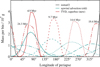 |
Fig. A.1 Azimuthal dispersion due to numerical limitations over time for the upwind advection scheme (blue-green) and the TVD scheme (red) with the superbee flux limiter. The labeled snapshots are isochronously separated by one-quarter of a full precession period. Equal styles of dashed lines correspond to equal times. The solid black line shows the initial distribution, scaled down by a factor of 1/2. Results are shown for a case with purely azimuthal precession: Mp = 2.5 MJup, ap = 20 au, ep = 0, ab = 102, eb = 0.31. |
Appendix B Observability of companion-induced shear
In this section we explore the feasibility of observing the features of our modeled planetary sheared debris disks as presented in Sects. 3 and 4 for an assumed distance of 7.7 pc (e.g., Fomalhaut) to the stellar system. In Fig. B.1, the same maps as in Fig. 9 are displayed, but with an absolute scale of surface brightness. Information about the corresponding dust masses is given in Sect. 3.1.
We investigated the potential of observing our simulated systems using JWST/NIRCam and ELT/MICADO at a wavelength of 2 µm, JWST/MIRI and ELT/METIS at 10 µm, JWST/MIRI at 21 µm, and Herschel/PACS at 70 µm. We estimated surface brightness sensitivities based on the literature and scaled them to the desired signal-to-noise ratio (S/N) and exposure time (texp) with the canonical relation, that the S/N is proportional to the square root of the exposure time and to the square root of the number of photons received.
JWST/NIRCam at 2 µm: To obtain an estimation of the surface brightness sensitivity we used the JWST exposure time calculator (Pontoppidan et al. 2016) in version 1.7. We employed a uniform brightness distribution, the preset readout pattern DEEP2, and a low background at the position of Fomalhaut. For the value of surface brightness we chose 5 × 10⁻⁷ Jy arcsec−2, a value intermediate for our systems (see the first panel of Fig. B.1a and B.1b, respectively). Using one exposure with six integrations of ten groups each we found an exposure time of texp ≈ 11780s ≈ 3.3h tobe sufficient to reach a S/N of 3.1. We neglected any influence by light not blocked or scattered of a possible coronagraph. The angular distance of disk emission to the position of the central star of several arcseconds is sufficiently large compared to the inner working angle of the suitable coronagraphic mask MASK210R, 0.40 arcsec (JWST Help Desk, priv. communication).
ELT/MICADO at 2 µm: Davies et al. (2018) expect the point-source sensitivity of ELT/MICADO to be comparable to the JWST, but with an angular size of one instrument pixel of 4 × 10⁻³ arcsec for the low resolution imager. Therefore, as for ELT/MICADO the angular area on the sky of one pixel is smaller than that of JWST/NIRCam6 by a factor of
 (B.1)
(B.1)
to detect a surface brightness of 5 × 10⁻⁷ Jy arcsec−2 with a S/N of 3, an exposure time of texp ≈ 186 h is required. Accordingly, to increase the S/N, a binning of several pixels will be required. To estimate the instrument performance in that case requires detailed modeling of the instrument noise. This is out of the scope of this estimation and we do not consider ELT/MICADO in the further analysis.
ELT/METIS at 10 µm: Brandl et al. (2021) denote for an observation with the N2 filter a required surface brightness sensitivity of 7.2 Jy arcsec−2 to achieve a S/N of 5 with an exposure time of 1 h. To detect our peak surface brightness of ~1 × 10⁻⁷ Jy arcsec−2 (see the second panel of Fig. B.1a and B.1b, respectively) with a S/N of 3 using ELT/METIS, an unfeasibly long exposure time would be required (~ yr). As for ELT/MICADO a binning of pixels will be required and we do not consider ELT/METIS in the further analysis.
JWST/MIRI at 10 µm and 21 µm: We follow the suggestions of the JWST Help Desk (priv. communication) and use the values of minimum detectable flux density for a S/N of 10 for an exposure time texp of 10 000 s, listed at the JWST User Documentation Webpage 7. These values are updated versions of the ones presented in Table 3 of Glasse et al. (2015) and will be updated during commissioning of the JWST. We selected the filters F1000W, F2100W for the wavelengths 10 µm, 21 µm and retrieved values of 0.52 × 10⁻⁶ Jy, 5.14 × 10⁻⁶ Jy, respectively. These values of sensitivity are valid for an unresolved point source. Using Eq. (12) from Glasse et al. (2015), which approximates the fraction of the total number of photons received by the central pixel, together with the field of view of a MIRI pixel of ≈0.012 arcsec2 we transformed these values to surface brightness sensitivities of ≈4.2 × 10⁻⁵ Jy arcsec−2, 4.2 × 10⁻⁴ Jy arcsec−2, respectively.
Like for the discussion of JWST/NIRCam, for this general and qualitative discussion of JWST/MIRI performance we neglected any influence of a possible coronagraph. The Lyot coronagraph of MIRI, especially suited for the observation of circumstellar disks, has an angular radius on the sky of 2.16 arcsec (Boccaletti et al. 2015). That is smaller by at least a factor of two than the angular distance of disk emission to central star in the investigated systems.
To detect our peak surface brightness of ~1 × 10⁻⁷ Jy arcsec−2 (see the second panel of Fig. B.1a and B.1b, respectively) with a S/N of 3 at a wavelength of 10 µm using JWST/MIRI an exposure time of texp ≈ 9 h is required.
At the wavelength of 21 µm, the situation is more favorable for JWST/MIRI than at 10 µm: For example, to detect intermediate surface brightness values of 5 × 10⁻⁵ Jy arcsec−2 (see the third panel of Fig. B.1a and B.1b, respectively) with a S/N of 3, an exposure time of ≈ 10 min is required.
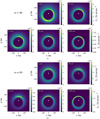 |
Fig. B.1 Surface brightness distributions of the systems n-i-M2 (a) and n-o-M3 (b) at the five wavelengths, 2 µm, 10 µm, 21 µm, 70 µm, and 1300 µm, zoomed in on the central ~ 190 au. The white asterisk denotes the position of the central star and defines the center of the coordinate system. Maps are the same as in Fig. 9, but now with the absolute scale of surface brightness for a stellar distance of 7.7 pc. |
Herschel/PACS at 70 µm: We adopt values from Table 1 of Acke et al. (2012), who observed the Fomalhaut debris disk: a surface brightness of ≈16.5 × 10⁻³ Jy arcsec−2 with a S/N of 77 and a total exposure time of texp = 10956 s. Based on these values and assuming a similar observing mode as it was used by Acke et al. (2012), our surface brightnesses at 70µm of ~5 × 10⁻³ Jy arcsec−2 are well detectable.
Appendix B.1 Twisting of the small grain halo
To illustrate the feasibility of characterizing the properties of the small grain halo, the values of surface brightness corresponding to the isophotes that are presented in Sect. 3.2 are displayed in Fig. B.2. Here we neglect the instrument PSF to keep this discussion independent from the distance to the system. We note that especially in the case of Herschel/PACS, convolving with the instruments PSF can significantly decrease the surface brightness of the systems. Additionally, horizontal lines indicate the surface brightnesses required to achieve a S/N of 3 and 5 for exposure times of texp = 1 h and 5 h. At the wavelength of 2 µm this is done for JWST/NIRCam, at 10 µm and 21 µm for JWST/MIRI, and at 70 µm for Herschel/PACS.
When observing at 2 µm with JWST/NIRCam, only the innermost parts of the halo can be detected with a S/N of at least 3 and an exposure time of texp = 5 h, while at 10 µm, the halo is too faint to be detected within that time. At the wavelength of 21 µm, substantial parts of the halo can be detected with JWST/MIRI. An observation with texp = 1 h is sufficient to detect emission with values of surface brightness corresponding to isophotes with semimajor axes of up to a ~ 140 au – 160 au with a S/N of 3. That allows halo regions undergoing differential rotation to be detected, but not those with flipping isophote orientation (see Fig. 12). To do so, five hours of observation time are required to detect emission with values of surface brightness corresponding to isophotes with semimajor axes of up to a ~ 190 au – 220 au with a S/N of 3, enough to measure almost the entire halo region undergoing that flip.
By observing at the wavelength of 70 µm with Herschel/PACS, major parts of the halo can be detected. An observation with texp = 1 h would have been sufficient to detect emission with values of surface brightness corresponding to isophotes with semimajor axes of up to a ~ 220 au – 240 au with a S/N of 3.
Appendix B.2 Spiral structure in the Q band
To illustrate the observability of the spiral structure appearing in the Q band (see Sect. 4.1), the surface brightness distribution of the system n-i-M4 such as in Fig. 13 is displayed in Fig. B.3, now convolved with a PSF suitable for JWST/MIRI. The PSF was calculated with version 1.0.0 of the tool WebbPSF8 (Perrin et al. 2012, 2014) using a flat input source for the filter F2100W. Beforehand, the surface brightness map was remapped to the JWST/MIRI pixel scale used by WebbPSF, which is 0.1108 arcsec. Overlaid on the surface brightness map are contour lines denoting significance regions for an exposure time of texp = 1 h. The whole area of the spiral structure can be measured with a S/N of more than 3 and most parts of it with a S/N of more than 5.
However, the contrast of the spiral structure would not be sufficient to detect the structure with such an observational setup. We assumed the structure to be detectable when the radial minimum and maxima producing the spiral structure have non overlapping noise intervals (computed by dividing the surface brightness by its S/N). Based on that assumption, an exposure time of texp > 8 h with JWST/MIRI would be required to significantly detect the spiral pattern for the system n-i-M4.
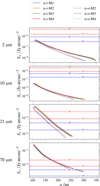 |
Fig. B.2 Brightness level of the isophotes used to trace the small grain halo (see Sect. 3.2) drawn over semimajor axis a. Solid lines are used for the systems with inner perturbers and dashed lines for those with outer perturbers, and rows are used to show four different wavelengths that trace small halo grains: 2 µm, 10 µm, 21 µm, and 70 µm. The horizontal dashed lines denote the minimum surface brightness required to achieve a certain detection significance (S/N), denoted by a multiple of the noise, σ. Red lines are for an exposure time of texp = 1 h, blue for texp = 5 h. For the wavelength of 2 µm the corresponding instrument is JWST/NIRCam, for 10 µm and 21 µm it is JWST/MIRI, and for 70 µm it is Herschel/PACS. |
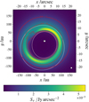 |
Fig. B.3 Surface brightness distribution for a stellar distance of 7.7 pc at a wavelength of 21 µm of the system n-i-M4, convolved with a PSF suitable for JWST/MIRI with the filter F2100W that has been obtained with the WebbPSF tool using a flat input source. To illustrate the PSF, a white circle is depicted in the lower-right edge with a diameter of 0.8″ (suitable for a wavelength of 21 µm and a telescope diameter of 6.5 m), similar to the used, more complex PSF. The red contour lines denote the regions succeeding the minimum surface brightness required to achieve a certain S/N when observing with JWST/MIRI for an exposure time of texp = 1 h. General figure characteristics are the same as in Fig. 9, and white contour lines have same meaning as in Fig. 13. |
Appendix B.3 Grains scattered inward of the parent planetesimal belt
The overall surface brightness of our systems is much higher at a wavelength of 21 µm than at 10 µm (see Fig. B.1, and Sect. 3.1 and Fig. 10 for the different contribution to surface brightness of different grain sizes). Therefore, we opt for 21 µm to illustrate the observability of emission from the region inward of the parent planetesimal belt (see Sect. 4.2) with JWST/MIRI. In Fig. B.4, the surface brightness map at 21 µm of the system n-o-M3 is displayed. The map has been treated the same way as Fig. B.3 as described in Sect. B.2. Evidently, with a exposure time of texp = 1 h using JWST/MIRI, the emission inside the belt can be detected with a S/N of at least 3 and mostly of at least 5.
Appendix B.4 Number of azimuthal radial flux maxima
We estimated the exposure time required to demarcate the second azimuthal maximum at θ ~ 240° from its consecutive minimum of the system n-i-M2 at the wavelength of 21 µm with JWST/MIRI. As in Sect. B.2 we assumed the structure to be detectable when the extrema values of surface brightnesses have non overlapping noise intervals. We found that an exposure time of texp ≈ 1 h would be sufficient to achieve that contrast.
References
- Acke, B., Min, M., Dominik, C., et al. 2012, A&A, 540, A125 [NASA ADS] [CrossRef] [EDP Sciences] [Google Scholar]
- Adam, C., Olofsson, J., van Holstein, R. G., et al. 2021, A&A, 653, A88 [NASA ADS] [CrossRef] [EDP Sciences] [Google Scholar]
- Arnold, J. A., Weinberger, A. J., Videen, G., & Zubko, E. S. 2019, AJ, 157, 157 [NASA ADS] [CrossRef] [Google Scholar]
- Astropy Collaboration (Robitaille, T. P., et al.) 2013, A&A, 558, A33 [NASA ADS] [CrossRef] [EDP Sciences] [Google Scholar]
- Astropy Collaboration (Price-Whelan, A. M., et al.) 2018, AJ, 156, 123 [Google Scholar]
- Beuzit, J. L., Vigan, A., Mouillet, D., et al. 2019, A&A, 631, A155 [NASA ADS] [CrossRef] [EDP Sciences] [Google Scholar]
- Boccaletti, A., Lagage, P. O., Baudoz, P., et al. 2015, PASP, 127, 633 [CrossRef] [Google Scholar]
- Boley, A. C., Payne, M. J., Corder, S., et al. 2012, ApJ, 750, L21 [NASA ADS] [CrossRef] [Google Scholar]
- Bowler, B. P. 2016, PASP, 128, 102001 [Google Scholar]
- Brandl, B. R., Feldt, M., Glasse, A., et al. 2014, SPIE Conf. Ser., 9147, 914721 [Google Scholar]
- Brandl, B., Bettonvil, F., van Boekel, R., et al. 2021, The Messenger, 182, 22 [NASA ADS] [Google Scholar]
- Bryan, M. L., Knutson, H. A., Howard, A. W., et al. 2016, ApJ, 821, 89 [NASA ADS] [CrossRef] [Google Scholar]
- Burns, J. A., Lamy, P. L., & Soter, S. 1979, Icarus, 40, 1 [Google Scholar]
- Campo Bagatin, A., Cellino, A., Davis, D. R., Farinella, P., & Paolicchi, P. 1994, Planet. Space Sci., 42, 1079 [NASA ADS] [CrossRef] [Google Scholar]
- Casertano, S., Lattanzi, M. G., Sozzetti, A., et al. 2008, A&A, 482, 699 [NASA ADS] [CrossRef] [EDP Sciences] [Google Scholar]
- Chatterjee, S., Ford, E. B., Matsumura, S., & Rasio, F. A. 2008, ApJ, 686, 580 [NASA ADS] [CrossRef] [Google Scholar]
- Davies, R., Alves, J., Clénet, Y., et al. 2018, SPIE Conf. Ser., 10702, 107021S [NASA ADS] [Google Scholar]
- Davies, R., Hörmann, V., Rabien, S., et al. 2021, The Messenger, 182, 17 [NASA ADS] [Google Scholar]
- Deeg, H. J., & Alonso, R. 2018, Transit Photometry as an Exoplanet Discovery Method, eds. H. J. Deeg, & J. A. Belmonte, 117 [Google Scholar]
- Draine, B. T. 2003, ApJ, 598, 1017 [NASA ADS] [CrossRef] [Google Scholar]
- Eiroa, C., Marshall, J. P., Mora, A., et al. 2013, A&A, 555, A11 [NASA ADS] [CrossRef] [EDP Sciences] [Google Scholar]
- Faramaz, V., Krist, J., Stapelfeldt, K. R., et al. 2019, AJ, 158, 162 [NASA ADS] [CrossRef] [Google Scholar]
- Gaia Collaboration (Prusti, T., et al.) 2016, A&A, 595, A1 [NASA ADS] [CrossRef] [EDP Sciences] [Google Scholar]
- Gardner, J. P., Mather, J. C., Clampin, M., et al. 2006, Space Sci. Rev., 123, 485 [Google Scholar]
- Garnett, J. C. M. 1904, Philos. Trans. Roy. Soc. Lond. A, 203, 385 [NASA ADS] [CrossRef] [Google Scholar]
- Glasse, A., Rieke, G. H., Bauwens, E., et al. 2015, PASP, 127, 686 [NASA ADS] [CrossRef] [Google Scholar]
- Gomes, R., Levison, H. F., Tsiganis, K., & Morbidelli, A. 2005, Nature, 435, 466 [Google Scholar]
- Gould, A., & Loeb, A. 1992, ApJ, 396, 104 [Google Scholar]
- Güttler, C., Blum, J., Zsom, A., Ormel, C. W., & Dullemond, C. P. 2010, A&A, 513, A56 [Google Scholar]
- Hahn, J. M. 2003, ApJ, 595, 531 [NASA ADS] [CrossRef] [Google Scholar]
- Harris, C. R., Millman, K. J., van der Walt, S. J., et al. 2020, Nature, 585, 357 [NASA ADS] [CrossRef] [Google Scholar]
- Harten, A. 1983, J. Comput. Phys., 49, 357 [Google Scholar]
- Hatzes, A. P., Cochran, W. D., McArthur, B., et al. 2000, ApJ, 544, L145 [Google Scholar]
- Hauschildt, P. H., Allard, F., & Baron, E. 1999, ApJ, 512, 377 [Google Scholar]
- Hedman, M. M., & Stark, C. C. 2015, ApJ, 811, 67 [NASA ADS] [CrossRef] [Google Scholar]
- Holland, W. S., Matthews, B. C., Kennedy, G. M., et al. 2017, MNRAS, 470, 3606 [NASA ADS] [CrossRef] [Google Scholar]
- Horner, S. D., & Rieke, M. J. 2004, SPIE Conf. Ser., 5487, 628 [NASA ADS] [Google Scholar]
- Hughes, A. M., Duchêne, G., & Matthews, B. C. 2018, ARA&A, 56, 541 [Google Scholar]
- Hunter, J. D. 2007, Comput. Sci. Eng., 9, 90 [NASA ADS] [CrossRef] [Google Scholar]
- Jackson, A. P., Wyatt, M. C., Bonsor, A., & Veras, D. 2014, MNRAS, 440, 3757 [NASA ADS] [CrossRef] [Google Scholar]
- Kalas, P., Graham, J. R., & Clampin, M. 2005, Nature, 435, 1067 [Google Scholar]
- Kalas, P., Graham, J. R., Fitzgerald, M. P., & Clampin, M. 2013, ApJ, 775, 56 [NASA ADS] [CrossRef] [Google Scholar]
- Kennedy, G. M. 2020, Roy. Soc. Open Sci., 7, 200063 [NASA ADS] [CrossRef] [Google Scholar]
- Kennedy, G. M., & Piette, A. 2015, MNRAS, 449, 2304 [NASA ADS] [CrossRef] [Google Scholar]
- Kennedy, G. M., Marino, S., Matrà, L., et al. 2018, MNRAS, 475, 4924 [Google Scholar]
- Kim, M., Wolf, S., Löhne, T., Kirchschlager, F., & Krivov, A. V. 2018, A&A, 618, A38 [NASA ADS] [CrossRef] [EDP Sciences] [Google Scholar]
- Kirchschlager, F., & Wolf, S. 2013, A&A, 552, A54 [NASA ADS] [CrossRef] [EDP Sciences] [Google Scholar]
- Kluyver, T., Ragan-Kelley, B., Pérez, F., et al. 2016, Jupyter Notebooks - A Publishing Format for Reproducible Computational Workflows, eds. F. Loizides, & B. Schmidt (Netherlands: IOS Press), 87 [Google Scholar]
- Kobayashi, H., & Ida, S. 2001, Icarus, 153, 416 [NASA ADS] [CrossRef] [Google Scholar]
- Kral, Q., Thébault, P., & Charnoz, S. 2013, A&A, 558, A121 [NASA ADS] [CrossRef] [EDP Sciences] [Google Scholar]
- Kral, Q., Thébault, P., Augereau, J. C., Boccaletti, A., & Charnoz, S. 2015, A&A, 573, A39 [NASA ADS] [CrossRef] [EDP Sciences] [Google Scholar]
- Krieger, A., & Wolf, S. 2022, A&A, 662, A99 [NASA ADS] [CrossRef] [EDP Sciences] [Google Scholar]
- Krijt, S., & Kama, M. 2014, A&A, 566, L2 [NASA ADS] [CrossRef] [EDP Sciences] [Google Scholar]
- Krist, J. E., Stapelfeldt, K. R., Bryden, G., & Plavchan, P. 2012, AJ, 144, 45 [NASA ADS] [CrossRef] [Google Scholar]
- Krivov, A. V. 2010, Res. Astron. Astrophys., 10, 383 [Google Scholar]
- Krivov, A. V., & Wyatt, M. C. 2021, MNRAS, 500, 718 [Google Scholar]
- Krivov, A. V., Sremčevič, M., & Spahn, F. 2005, Icarus, 174, 105 [NASA ADS] [CrossRef] [Google Scholar]
- Krivov, A. V., Löhne, T., & Sremčevič, M. 2006, A&A, 455, 509 [NASA ADS] [CrossRef] [EDP Sciences] [Google Scholar]
- Krivov, A. V., Queck, M., Löhne, T., & Sremčevič, M. 2007, A&A, 462, 199 [NASA ADS] [CrossRef] [EDP Sciences] [Google Scholar]
- Krivov, A. V., Ide, A., Löhne, T., Johansen, A., & Blum, J. 2018, MNRAS, 474, 2564 [NASA ADS] [CrossRef] [Google Scholar]
- Kurz, R., Guilloteau, S., & Shaver, P. 2002, The Messenger, 107, 7 [NASA ADS] [Google Scholar]
- Lagrange, A. M., Gratadour, D., Chauvin, G., et al. 2009, A&A, 493, L21 [NASA ADS] [CrossRef] [EDP Sciences] [Google Scholar]
- Lagrange, A. M., Bonnefoy, M., Chauvin, G., et al. 2010, Science, 329, 57 [Google Scholar]
- Lagrange, A. M., Meunier, N., Rubini, P., et al. 2019, Nat. Astron., 3, 1135 [NASA ADS] [CrossRef] [Google Scholar]
- Larwood, J. D., & Kalas, P. G. 2001, MNRAS, 323, 402 [NASA ADS] [CrossRef] [Google Scholar]
- Le Bouquin, J. B., Absil, O., Benisty, M., et al. 2009, A&A, 498, L41 [NASA ADS] [CrossRef] [EDP Sciences] [Google Scholar]
- Lee, E. J., & Chiang, E. 2016, ApJ, 827, 125 [NASA ADS] [CrossRef] [Google Scholar]
- Levison, H. F., Duncan, M. J., & Thommes, E. 2012, AJ, 144, 119 [NASA ADS] [CrossRef] [Google Scholar]
- Li, A., & Greenberg, J. M. 1998, A&A, 331, 291 [NASA ADS] [Google Scholar]
- Löhne, T., Augereau, J. C., Ertel, S., et al. 2012, A&A, 537, A110 [NASA ADS] [CrossRef] [EDP Sciences] [Google Scholar]
- Löhne, T., Krivov, A. V., Kirchschlager, F., Sende, J. A., & Wolf, S. 2017, A&A, 605, A7 [Google Scholar]
- Lovis, C., & Fischer, D. 2010, Radial Velocity Techniques for Exoplanets, ed. S. Seager (Tucson, AZ: University of Arizona Press), 27 [Google Scholar]
- MacGregor, M. A., Matrà, L., Kalas, P., et al. 2017, ApJ, 842, 8 [CrossRef] [Google Scholar]
- MacGregor, M. A., Hurt, S. A., Stark, C. C., et al. 2022, ApJ, 933, L1 [NASA ADS] [CrossRef] [Google Scholar]
- Maldonado, J., Eiroa, C., Villaver, E., Montesinos, B., & Mora, A. 2012, A&A, 541, A40 [NASA ADS] [CrossRef] [EDP Sciences] [Google Scholar]
- Maldonado, J., Eiroa, C., Villaver, E., Montesinos, B., & Mora, A. 2015, A&A, 579, A20 [NASA ADS] [CrossRef] [EDP Sciences] [Google Scholar]
- Mann, I., Köhler, M., Kimura, H., Cechowski, A., & Minato, T. 2006, A&Ar, 13, 159 [NASA ADS] [CrossRef] [Google Scholar]
- Mao, S. 2012, Res. Astron. Astrophys., 12, 947 [Google Scholar]
- Mao, S., & Paczynski, B. 1991, ApJ, 374, L37 [NASA ADS] [CrossRef] [Google Scholar]
- Marino, S. 2021, MNRAS, 503, 5100 [NASA ADS] [CrossRef] [Google Scholar]
- Marshall, J. P., Moro-Martín, A., Eiroa, C., et al. 2014, A&A, 565, A15 [NASA ADS] [CrossRef] [EDP Sciences] [Google Scholar]
- Marshall, J. P., Wang, L., Kennedy, G. M., Zeegers, S. T., & Scicluna, P. 2021, MNRAS, 501, 6168 [NASA ADS] [CrossRef] [Google Scholar]
- Martioli, E., Hébrard, G., Correia, A. C. M., Laskar, J., & Lecavelier des Etangs, A. 2021, A&A, 649, A177 [NASA ADS] [CrossRef] [EDP Sciences] [Google Scholar]
- Matrà, L., Marino, S., Kennedy, G. M., et al. 2018, ApJ, 859, 72 [Google Scholar]
- Matthews, B. C., Krivov, A. V., Wyatt, M. C., Bryden, G., & Eiroa, C. 2014, in Protostars and Planets VI, eds. H. Beuther, R. S. Klessen, C. P. Dullemond, & T. Henning, 521 [Google Scholar]
- Mie, G. 1908, Ann. Phys., 330, 377 [Google Scholar]
- Milli, J., Vigan, A., Mouillet, D., et al. 2017, A&A, 599, A108 [NASA ADS] [CrossRef] [EDP Sciences] [Google Scholar]
- Min, M., Kama, M., Dominik, C., & Waters, L. B. F. M. 2010, A&A, 509, A6 [NASA ADS] [CrossRef] [EDP Sciences] [Google Scholar]
- Moerchen, M. M., Churcher, L. J., Telesco, C. M., et al. 2011, A&A, 526, A34 [NASA ADS] [CrossRef] [EDP Sciences] [Google Scholar]
- Montesinos, B., Eiroa, C., Krivov, A. V., et al. 2016, A&A, 593, A51 [NASA ADS] [CrossRef] [EDP Sciences] [Google Scholar]
- Morales, F. Y., Bryden, G., Werner, M. W., & Stapelfeldt, K. R. 2013, ApJ, 776, 111 [NASA ADS] [CrossRef] [Google Scholar]
- Morales, F. Y., Bryden, G., Werner, M. W., & Stapelfeldt, K. R. 2016, ApJ, 831, 97 [Google Scholar]
- Nesvold, E. R., Kuchner, M. J., Rein, H., & Pan, M. 2013, ApJ, 777, 144 [NASA ADS] [CrossRef] [Google Scholar]
- Nowak, M., Lacour, S., Lagrange, A. M., et al. 2020, A&A, 642, A2 [NASA ADS] [CrossRef] [EDP Sciences] [Google Scholar]
- O’Brien, D. P., & Greenberg, R. 2003, Icarus, 164, 334 [CrossRef] [Google Scholar]
- Olofsson, J., Milli, J., Bayo, A., Henning, T., & Engler, N. 2020, A&A, 640, A12 [NASA ADS] [CrossRef] [EDP Sciences] [Google Scholar]
- Pan, M., Nesvold, E. R., & Kuchner, M. J. 2016, ApJ, 832, 81 [NASA ADS] [CrossRef] [Google Scholar]
- Pawellek, N., Krivov, A. V., Marshall, J. P., et al. 2014, ApJ, 792, 65 [Google Scholar]
- Pearce, T. D., & Wyatt, M. C. 2015, MNRAS, 453, 3329 [Google Scholar]
- Pearce, T. D., Beust, H., Faramaz, V., et al. 2021, MNRAS, 503, 4767 [Google Scholar]
- Pearce, T. D., Launhardt, R., Ostermann, R., et al. 2022, A&A, 659, A135 [NASA ADS] [CrossRef] [EDP Sciences] [Google Scholar]
- Perez, F., & Granger, B. E. 2007, Comput. Sci. Eng., 9, 21 [Google Scholar]
- Perrin, M. D., Soummer, R., Elliott, E. M., Lallo, M. D., & Sivaramakrishnan, A. 2012, SPIE Conf. Ser., 8442, 84423D [NASA ADS] [Google Scholar]
- Perrin, M. D., Sivaramakrishnan, A., Lajoie, C.-P., et al. 2014, SPIE Conf. Ser., 9143, 91433X [NASA ADS] [Google Scholar]
- Perryman, M., Hartman, J., Bakos, G. Á., & Lindegren, L. 2014, ApJ, 797, 14 [Google Scholar]
- Pilbratt, G. L., Riedinger, J. R., Passvogel, T., et al. 2010, A&A, 518, L1 [NASA ADS] [CrossRef] [EDP Sciences] [Google Scholar]
- Plavchan, P., Barclay, T., Gagné, J., et al. 2020, Nature, 582, 497 [Google Scholar]
- Poglitsch, A., Waelkens, C., Geis, N., et al. 2010, A&A, 518, A2 [Google Scholar]
- Pontoppidan, K. M., Pickering, T. E., Laidler, V. G., et al. 2016, SPIE Conf. Ser., 9910, 991016 [NASA ADS] [Google Scholar]
- Quillen, A. C., Varnière, P., Minchev, I., & Frank, A. 2005, AJ, 129, 2481 [NASA ADS] [CrossRef] [Google Scholar]
- Ranalli, P., Hobbs, D., & Lindegren, L. 2018, A&A, 614, A30 [NASA ADS] [CrossRef] [EDP Sciences] [Google Scholar]
- Reche, R., Beust, H., Augereau, J. C., & Absil, O. 2008, A&A, 480, 551 [NASA ADS] [CrossRef] [EDP Sciences] [Google Scholar]
- Reidemeister, M., Krivov, A. V., Stark, C. C., et al. 2011, A&A, 527, A57 [NASA ADS] [CrossRef] [EDP Sciences] [Google Scholar]
- Rodet, L., & Lai, D. 2022, MNRAS, 516, 5544 [NASA ADS] [CrossRef] [Google Scholar]
- Roe, P. L. 1986, Annu. Rev. Fluid Mech., 18, 337 [NASA ADS] [CrossRef] [Google Scholar]
- Schneider, G., Grady, C. A., Stark, C. C., et al. 2016, AJ, 152, 64 [NASA ADS] [CrossRef] [Google Scholar]
- Schüppler, C., Löhne, T., Krivov, A. V., et al. 2014, A&A, 567, A127 [NASA ADS] [CrossRef] [EDP Sciences] [Google Scholar]
- Sefilian, A. A., Rafikov, R. R., & Wyatt, M. C. 2021, ApJ, 910, 13 [NASA ADS] [CrossRef] [Google Scholar]
- Sende, J. A., & Löhne, T. 2019, A&A, 631, A141 [NASA ADS] [CrossRef] [EDP Sciences] [Google Scholar]
- Sibthorpe, B., Kennedy, G. M., Wyatt, M. C., et al. 2018, MNRAS, 475, 3046 [Google Scholar]
- Stark, C. C., & Kuchner, M. J. 2009, ApJ, 707, 543 [Google Scholar]
- Struve, O. 1952, The Observatory, 72, 199 [Google Scholar]
- Su, K. Y. L., Rieke, G. H., Stansberry, J. A., et al. 2006, ApJ, 653, 675 [Google Scholar]
- Thébault, P. 2012, A&A, 537, A65 [Google Scholar]
- Thebault, P. 2016, A&A, 587, A88 [NASA ADS] [CrossRef] [EDP Sciences] [Google Scholar]
- Thébault, P., & Augereau, J. C. 2007, A&A, 472, 169 [NASA ADS] [CrossRef] [EDP Sciences] [Google Scholar]
- Thébault, P., Augereau, J. C., & Beust, H. 2003, A&A, 408, 775 [NASA ADS] [CrossRef] [EDP Sciences] [Google Scholar]
- Thébault, P., Marzari, F., & Scholl, H. 2006, Icarus, 183, 193 [Google Scholar]
- Thebault, P., Kral, Q., & Ertel, S. 2012, A&A, 547, A92 [NASA ADS] [CrossRef] [EDP Sciences] [Google Scholar]
- Tsapras, Y. 2018, Geosciences, 8, 365 [NASA ADS] [CrossRef] [Google Scholar]
- van der Walt, S., Schönberger, J. L., Nunez-Iglesias, J., et al. 2014, PeerJ, 2, e453 [Google Scholar]
- Virtanen, P., Gommers, R., Oliphant, T. E., et al. 2020, Nat. Methods, 17, 261 [Google Scholar]
- Vitense, C., Krivov, A. V., & Löhne, T. 2010, A&A, 520, A32 [NASA ADS] [CrossRef] [EDP Sciences] [Google Scholar]
- Wolf, S., & Voshchinnikov, N. V. 2004, Comput. Phys. Commun., 162, 113 [Google Scholar]
- Wolf, S., Moro-Martín, A., & D’Angelo, G. 2007, Planet. Space Sci., 55, 569 [NASA ADS] [CrossRef] [Google Scholar]
- Wright, G. S., Rieke, G. H., Colina, L., et al. 2004, SPIE Conf. Ser., 5487, 653 [NASA ADS] [Google Scholar]
- Wyatt, M. C. 2003, ApJ, 598, 1321 [NASA ADS] [CrossRef] [Google Scholar]
- Wyatt, M. C. 2005a, A&A, 440, 937 [NASA ADS] [CrossRef] [EDP Sciences] [Google Scholar]
- Wyatt, M. C. 2005b, A&A, 433, 1007 [NASA ADS] [CrossRef] [EDP Sciences] [Google Scholar]
- Wyatt, M. C. 2006, ApJ, 639, 1153 [NASA ADS] [CrossRef] [Google Scholar]
- Wyatt, M. 2020, in The Trans-Neptunian Solar System, eds. D. Prialnik, M. A. Barucci, & L. Young (Elsevier), 351 [CrossRef] [Google Scholar]
- Wyatt, M. C., & Jackson, A. P. 2016, Space Sci. Rev., 205, 231 [NASA ADS] [CrossRef] [Google Scholar]
- Wyatt, M. C., Dermott, S. F., Telesco, C. M., et al. 1999, ApJ, 527, 918 [Google Scholar]
- Yelverton, B., & Kennedy, G. M. 2018, MNRAS, 479, 2673 [NASA ADS] [CrossRef] [Google Scholar]
We used units of flux density per grid cell area, that is, Jy arcsec−2. Thus, the quantities are independent of the grid cell area, which varies drastically in a polar grid.
We used the routine from https://scipython.com/book/chapter-8-scipy/examples/non-linear-fitting-to-an-ellipse/, extended by the position angle of the periapse ϕ.
Using the canonical celestial directions for images on the sky and hence north is up and west is to the right.
All Tables
All Figures
|
Fig. 1 Schematic representation of the belt orbits (solid gray and black) and the planet orbit (red) at the different stages of the ACE simulations: (a) the initial, circular, unperturbed belt; (a, b) the belt perturbed by the planet, but not modified by collisions; (b) the belt modified by collisions, but not by the perturber; (b, c) the belt modified by both the perturber and collisions. |
| In the text | |
|
Fig. 2 Maps of contributions to face-on optical depth, τ, in run n-i-M2 from grains of four different size bins with mean grain radii s and corresponding β ratios, as labeled in the top-left corners of the panels. The orbits of the perturbers are shown with blue-green ellipses, and the host star is at the crossings of the major axes and latera recta. Dashed black-and-white ellipses trace the center of the parent belt. White lines show the orientations and lengths of the pericenters at the belt center (solid) and the belt edges (dashed). Arrows indicate the scale. |
| In the text | |
|
Fig. 3 Size dependence of timescales for collisions (solid blue, green, and red), PR drag (solid black), and a full secular precession cycle at 100 au (dashed black) for perturbers of different masses, as labeled. The timescales are calculated as described in Sende & Löhne (2019). |
| In the text | |
|
Fig. 4 Maps of contributions to face-on optical depth for grains of radius s = 5 mm in four different simulation runs: (a) n-i-M2, (b)n-p0, (c) n-o-M3, and (d) w-i-M2. See Fig. 2 for a detailed description. |
| In the text | |
|
Fig. 5 Maps of contributions to face-on optical depth for grains of radius s = 7.5 µm in six different simulation runs: (a) n-i-M2, (b) n-di, (c) n-pβ, (d) n-o-M3, (e) n-p1, and (f) W-1-M2. See Fig. 2 for a detailed description. |
| In the text | |
|
Fig. 6 Maps of contributions to face-on optical depth for grains of radius s = 7.5 µm in runs: (a) n-i-M1, (b) n-i-M2, (c) n-i-M3, and (d) n-i-M4. See Fig. 2 for a detailed description. |
| In the text | |
|
Fig. 7 Azimuthalfy averaged grain size distributions in terms of contribution to normal optical thickness at 100 au (left) and 200 au (right) for runs n-i-M1 (red), n-i-M2 (green), n-i-M3 (blue), and n-i-M4 (black). The dashed line traces the initial distribution common to all runs, with a lower radius limit at 100 µm. The gray-shaded region is dominated by grains on unbound orbits. |
| In the text | |
|
Fig. 8 Maps of contributions to face-on optical depth for grains of radii s = 7.5 µm (a) and s = 5 mm (b) in run n-M2-1e. |
| In the text | |
|
Fig. 9 Surface brightness distributions of the system with parent belt n and perturber i-M2 orbiting inside the belt (n-i-M2; top row) and the system with belt n and perturber o-M3 orbiting outside the belt (n-o-M3; bottom row) for a stellar distance of 7.7 pc at five wavelengths: 2 µm, 10 µm, 21 µm, 70 µm, and 1300 µm (from left to right), zoomed in on the central ~190 au. Each distribution has been normalized by its respective maximum value, Sv,max. The white asterisk denotes the position of the central star and defines the center of the coordinate system. |
| In the text | |
|
Fig. 10 Radial brightness profiles normalized by their respective maximum value, Sv,rp,max, at the wavelengths 2 µm, 10 µm, 21 µm, and 70 µm of the system with the reference planetesimal belt n and the i-M2 inner perturber (n-i-M2). The dotted blue line shows the relative contribution of radiation from grains with radii s ≤ 4.9 µm, the dashed orange line of grains with radii s ≥ 6.1 µm, and the solid black line shows the total emission as the sum of the two fractions. The radial profiles of each wavelength are normalized to the maximum value of the respective total brightness profile. |
| In the text | |
|
Fig. 11 Polar brightness maps of the systems n-i-M2 (same as in Fig. B.1a) and n-o-M4 at a wavelength of 2 µm (radius 400 au). The white asterisk denotes the position of the central star and defines the center of the coordinate system. The white crosses trace five lines of constant brightness (isophotes) and are drawn every 7.5°. The colored ellipses have been fitted to the respective isophotes using Eq. (4) with the central star in one of the focal points. The dashed lines give the direction from the focal point to the periapse, that is, ϕ + π, and are drawn in the same color as their corresponding ellipse. |
| In the text | |
|
Fig. 12 Orientation, ∆ϕ, of the isophote ellipses relative to the orientation of the innermost ellipse drawn over semimajor axis a. A negative value of ∆ϕ means clockwise rotation and a positive value counterclockwise rotation. Solid lines are used for the systems with inner perturbers and dashed lines for those with outer perturbers, and rows are used to show four different wavelengths tracing small halo grains: 2 µm, 10 µm, 21 µm, and 70 µm. |
| In the text | |
|
Fig. 13 Surface brightness distribution for a stellar distance of 7.7 pc at the wavelength 21 µm (Q band) of the system with belt parameter set n and the inner perturber i-M4 (n-i-M4). The contour lines denote the isophotes of the corresponding 1300 µm map of the same system with a flux density level of 1 % of its maximum value. They enclose the position of the parent planetesimal belt. General figure characteristics are the same as in Fig. 9. |
| In the text | |
|
Fig. 14 Surface brightness distribution for a stellar distance of 7.7 pc at the wavelength 10 µm (N band) of the system with belt parameter set n and the outer perturber o-M3 (n-o-M3). General figure characteristics are the same as in Fig. 9, and white contour lines have the same meaning as in Fig. 13. |
| In the text | |
|
Fig. 15 Azimuthal distribution of radial maxima of brightness normalized by their respective maximum value, Sv,max, in the five investigated wavelengths: 2 µm, 10 µm, 21 µm, 70 µm, and 1300 µm. Left: Systems with an inner perturber. System n-p1 is displayed as a reference that shows the case without ongoing precession. Right: Systems with an outer perturber. |
| In the text | |
|
Fig. 16 Flowchart for deciding whether an inner or outer perturber orbits in the system based on distinct observable features of a debris disk system. |
| In the text | |
|
Fig. A.1 Azimuthal dispersion due to numerical limitations over time for the upwind advection scheme (blue-green) and the TVD scheme (red) with the superbee flux limiter. The labeled snapshots are isochronously separated by one-quarter of a full precession period. Equal styles of dashed lines correspond to equal times. The solid black line shows the initial distribution, scaled down by a factor of 1/2. Results are shown for a case with purely azimuthal precession: Mp = 2.5 MJup, ap = 20 au, ep = 0, ab = 102, eb = 0.31. |
| In the text | |
|
Fig. B.1 Surface brightness distributions of the systems n-i-M2 (a) and n-o-M3 (b) at the five wavelengths, 2 µm, 10 µm, 21 µm, 70 µm, and 1300 µm, zoomed in on the central ~ 190 au. The white asterisk denotes the position of the central star and defines the center of the coordinate system. Maps are the same as in Fig. 9, but now with the absolute scale of surface brightness for a stellar distance of 7.7 pc. |
| In the text | |
|
Fig. B.2 Brightness level of the isophotes used to trace the small grain halo (see Sect. 3.2) drawn over semimajor axis a. Solid lines are used for the systems with inner perturbers and dashed lines for those with outer perturbers, and rows are used to show four different wavelengths that trace small halo grains: 2 µm, 10 µm, 21 µm, and 70 µm. The horizontal dashed lines denote the minimum surface brightness required to achieve a certain detection significance (S/N), denoted by a multiple of the noise, σ. Red lines are for an exposure time of texp = 1 h, blue for texp = 5 h. For the wavelength of 2 µm the corresponding instrument is JWST/NIRCam, for 10 µm and 21 µm it is JWST/MIRI, and for 70 µm it is Herschel/PACS. |
| In the text | |
|
Fig. B.3 Surface brightness distribution for a stellar distance of 7.7 pc at a wavelength of 21 µm of the system n-i-M4, convolved with a PSF suitable for JWST/MIRI with the filter F2100W that has been obtained with the WebbPSF tool using a flat input source. To illustrate the PSF, a white circle is depicted in the lower-right edge with a diameter of 0.8″ (suitable for a wavelength of 21 µm and a telescope diameter of 6.5 m), similar to the used, more complex PSF. The red contour lines denote the regions succeeding the minimum surface brightness required to achieve a certain S/N when observing with JWST/MIRI for an exposure time of texp = 1 h. General figure characteristics are the same as in Fig. 9, and white contour lines have same meaning as in Fig. 13. |
| In the text | |
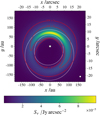 |
Fig. B.4 Same as Fig. B.3, but for the system n-o-M3. |
| In the text | |
Current usage metrics show cumulative count of Article Views (full-text article views including HTML views, PDF and ePub downloads, according to the available data) and Abstracts Views on Vision4Press platform.
Data correspond to usage on the plateform after 2015. The current usage metrics is available 48-96 hours after online publication and is updated daily on week days.
Initial download of the metrics may take a while.