| Issue |
A&A
Volume 668, December 2022
|
|
|---|---|---|
| Article Number | A176 | |
| Number of page(s) | 22 | |
| Section | Planets and planetary systems | |
| DOI | https://doi.org/10.1051/0004-6361/202244593 | |
| Published online | 21 December 2022 | |
The GAPS Programme at TNG
XLI. The climate of KELT-9b revealed with a new approach to high-spectral-resolution phase curves
1
INAF – Osservatorio Astrofísico di Arcetri,
Largo Enrico Fermi 5,
50125
Firenze, Italy
e-mail: This email address is being protected from spambots. You need JavaScript enabled to view it.
2
Department of Physics, University of Warwick,
Coventry,
CV4 7AL, UK
3
INAF – Osservatorio Astrofísico di Torino,
Via Osservatorio 20,
10025,
Pino Torinese, Italy
4
Centre for Exoplanets and Habitability, University of Warwick,
Coventry,
CV4 7AL, UK
5
Anton Pannekoek Institute for Astronomy, University of Amsterdam,
1098 XH
Amsterdam, The Netherlands
6
INAF – Osservatorio Astronomico di Padova,
Padova
35122, Italy
7
Department of Astronomy, University of Michigan,
Ann Arbor, MI
48109, USA
8
Department of Physics, University of Rome “Tor Vergata”,
Via della Ricerca Scientifica 1,
00133
Rome, Italy
9
INAF – Osservatorio Astrofísico di Catania,
Via Santa Sofia 78,
95123
Catania, Italy
10
INAF – Osservatorio Astronomico di Trieste,
via Tiepolo 11,
34143
Trieste, Italy
11
INAF – Osservatorio Astronomico di Brera,
Via E. Bianchi 46,
23807
Merate, Italy
12
INAF – Osservatorio Astronomico di Capodimonte,
Salita Moiariello 16,
80131
Napoli, Italy
13
INAF – IAPS Istituto di Astrofísica e Planetologia Spaziali,
Via del Fosso del Cavaliere 100,
00133
Roma, Italy
14
INAF – Osservatorio Astronomico di Palermo,
Piazza del Parlamento, 1,
90134
Palermo, Italy
15
Dip. di Fisica e Astronomia Galileo Galilei – Università di Padova,
Vicolo dell'Osservatorio 2,
35122
Padova, Italy
16
INAF – Osservatorio di Cagliari,
via della Scienza 5,
09047
Selargius, Italy
17
Aix Marseille Univ, CNRS, CNES, LAM,
13388
Marseille, France
18
Fundación Galileo Galilei – INAF,
Rambla José Ana Fernandez Pérez 7,
38712
Brena Baja, TF, Spain
Received:
25
July
2022
Accepted:
25
September
2022
Abstract
Aims. We present a novel method for studying the thermal emission of exoplanets as a function of orbital phase at very high spectral resolution, and use it to investigate the climate of the ultra-hot Jupiter KELT-9b.
Methods. We combine three nights of HARPS-N and two nights of CARMENES optical spectra, covering orbital phases between quadratures (0.25 < φ < 0.75), when the planet shows its day-side hemisphere with different geometries. We co-add the signal of thousands of Fe I lines through cross-correlation, which we map to a likelihood function. We investigate the phase-dependence of two separate observable quantities, namely (i) the line depths of Fe I and (ii) their Doppler shifts, introducing a new method that exploits the very high spectral resolution of our observations.
Results. We confirm a previous detection of Fe I emission, and demonstrate a precision of 0.5 km s−1 on the orbital properties of KELT-9b when combining all nights of observations. By studying the phase-resolved Doppler shift of Fe I lines, we detect an anomaly in the planet's orbital radial velocity well-fitted with a slightly eccentric orbital solution (e = 0.016 ± 0.003, ω = 150−11+13°, 5σ preference). However, we argue that this anomaly is caused by atmospheric circulation patterns, and can be explained if neutral iron gas is advected by day-to-night atmospheric wind flows of the order of a few km s−1. We additionally show that the Fe I emission line depths are symmetric around the substellar point within 10° (2σ), possibly indicating the lack of a large hot-spot offset at the altitude probed by neutral iron emission lines. Finally, we do not obtain a significant preference for models with a strong phase-dependence of the Fe I emission line strength. We show that these results are qualitatively compatible with predictions from general circulation models (GCMs) for ultra-hot Jupiter planets.
Conclusions. Very high-resolution spectroscopy phase curves are of sufficient sensitivity to reveal a phase dependence in both the line depths and their Doppler shifts throughout the orbit. They constitute an under-exploited treasure trove of information that is highly complementary to space-based phase curves obtained with HST and JWST, and open a new window onto the still poorly understood climate and atmospheric structure of the hottest planets known to date.
Key words: planets and satellites: atmospheres / planets and satellites: composition / techniques: spectroscopic / radiative transfer
© L. Pino et al. 2022
 Open Access article, published by EDP Sciences, under the terms of the Creative Commons Attribution License (https://creativecommons.org/licenses/by/4.0), which permits unrestricted use, distribution, and reproduction in any medium, provided the original work is properly cited.
This article is published in open access under the Subscribe-to-Open model. This email address is being protected from spambots. You need JavaScript enabled to view it. to support open access publication.
1 Introduction
Ultra-hot Jupiters (UHJs) are gas giants with orbital periods of hours to days and typical day-side temperatures of 2500 K or more. They form a continuum with the broader population of hot Jupiters, of which they constitute the high temperature end (Baxter et al. 2020; Mansfield et al. 2021). As a result of their temperatures, which push towards stellar values, they have distinct atmospheric properties that make them ideal laboratories for studying atmospheric physics and chemistry in a unique regime of temperature and pressure. Indeed, their daysides are expected to be cloud free and close to chemical equilibrium (Kitzmann et al. 2018; Lothringer et al. 2018; Parmentier et al. 2018; Helling et al. 2019). Clouds may still form on their night-side, but they do not completely sequester heavy elements, which are present in their transmission (e.g. Hoeijmakers et al. 2018) and emission spectra (e.g. Pino et al. 2020). As a result, UHJs currently constitute the only class of planets for which it is possible to measure the abundances of elements with different volatilities, including rock-forming elements. This makes UHJs very promising benchmarks for planet formation theories (Lothringer et al. 2021).
Observational campaigns employing a variety of instruments, both from the ground and in space, have so far mainly focused on the dayside (through emission spectroscopy) and terminator regions (through transmission spectroscopy) of UHJs, because these yield the best signal-to-noise ratio (S/N). These methods have been successful in probing the local properties of their atmospheres. However, because of their short orbital periods, UHJs are expected to be tidally locked. Therefore, the global properties of UHJ atmospheres may deviate from the local ones, and it is necessary to account for three-dimensional (3D) effects (e.g. Feng et al. 2016). Observationally, this has so far been best achieved through phase curves.
Phase curves record the flux emitted from the planet throughout the orbit. In photometry, a relative calibration to the stellar flux registered during the secondary eclipse permits the measurement of the phase-resolved effective temperature of the planet – including its day-to-night contrast – and the longitude of its atmospheric hot spot. When observed through a low-resolution spectrograph (e.g. HST WFC3), the resulting spectrophotometric phase curve can be used to resolve these properties in altitude, and can additionally reveal the phase-dependent chemistry (Stevenson et al. 2014; Mikal-Evans et al. 2022).
Multi-wavelength photometric phase curves have been obtained for tens of hot and ultra-hot Jupiters and spectrophotometric phase curves are also available for a handful of them. These observations have revealed that the climate of UHJs may differ from that of their cooler counterparts. Relatively small hot-spot offsets and small day-to-night contrasts (albeit observed with some scatter) indicate that UHJs may not develop strong equatorial jets, but heat transport from day to night is still efficient (Parmentier & Crossfield 2018). These observations contrast with trends observed for gas giants colder than 2500 K (Zhang et al. 2018; Wong et al. 2020), which have weaker hotspot offsets but, unlike their hotter counter-parts, display larger day-to-night contrasts with increasing temperature, indicating a reduced heat transport efficiency. Theoretical studies led to the identification of two key additional ingredients that emerge in UHJs and are necessary to explain their different climate: thermal recombination of atomic hydrogen to H2 on their nightside, which leads to an increase in the efficiency of heat transport (Bell & Cowan 2018), and atmospheric drag, which affects their atmospheric circulation patterns. Indeed, the interaction of the significant planetary ionospheres – produced by the high temperatures – and magnetic fields can lead to dampening of the waves that would otherwise trigger the formation of an equatorial jet (Perna et al. 2010; Beltz et al. 2022b). This would give rise to smaller hot-spot offsets, and potentially to a transition to day-to-night atmospheric flow (Tan & Komacek 2019). While this theory has been shown to be moderately successful in explaining the overall properties of the climate of UHJs, results obtained on individual UHJs do not perfectly support this scenario (e.g. Addison et al. 2021). Reconciling optical (e.g. Transiting Exoplanet Survey Satellite; TESS) and infrared (IR; e.g. Spitzer) phase curves proves particularly challenging in some cases (Wong et al. 2020; von Essen et al. 2020).
Very high-resolution spectroscopy (HRS; R ≳ 100 000) offers a unique observational angle from which to tackle the open questions in this field. Indeed, by individually resolving spectral lines, HRS is able to directly measure the Doppler-shift of spectral lines, and thus probe the strength of winds moving masses of gas around the atmosphere of target planets. Ehrenreich et al. (2020) showcased the power of this technique by measuring phase-resolved transmission spectroscopy of UHJ WASP-76b. These authors reveal a complex Doppler shift pattern that is sensitive to temperature structure, rotation, dynamics, and nightside condensation (Wardenier et al. 2021; Savel et al. 2022). However, HRS transmission spectra generally probe altitudes above the planet photosphere (e.g. Hoeijmakers et al. 2019), and can only access a limited longitudinal region of the planetary atmosphere (Wardenier et al. 2022).
A complementary approach is to observe parts of a planetary phase curve with a high-resolution spectrograph. When observed using this technique, features in the planet continuum are lost, but the phase-resolved Doppler shift and Doppler broadening of emission or reflection lines uniquely constrains the orbit of the planet, as well as its rotation and dynamics (Collier Cameron et al. 1999; Kawahara 2012; Brogi et al. 2013; Snellen et al. 2014). This is supported by dedicated theoretical studies, which, applying radiative transfer to general circulation models (GCMs), show that the combination of inhomogeneous specific intensity, rotation, and winds imprints kilometre-per-second level Doppler shifts and significant distortions in the line shapes and strengths (Zhang et al. 2017; Beltz et al. 2022a). However, two challenges have so far hindered the use of this technique. First, the signal observed in this configuration is weaker compared to transmission spectroscopy, which has led most authors to stack spectra across planet phases to increase the significance of detections. Unfortunately, this operation washes out the phase-dependency of the line profiles, which is crucial to probing planetary climate. Second, HRS observations require complex data-reduction methods, which makes the retrieval of atmospheric properties a non-trivial operation.
Both challenges can now be surpassed. Recently developed likelihood-based frameworks (Brogi & Line 2019; Gibson et al. 2020; Pino et al. 2020) allow us to reliably determine atmospheric properties and their error bars starting from HRS emission spectra. Exploiting this key technical novelty, Beltz et al. (2021) presented the first indication that the HRS phase curve of HD 209458b observed with the CRyogenic high-resolution InfraRed Echelle Spectrograph (CRIRES) has the sensitivity to probe 3D effects in the planetary atmosphere. In addition, thanks to their relatively large planet-to-star flux ratio, UHJs offer the opportunity to observe HRS phase curves at unprecedented S/N. Indeed, Herman et al. (2022) and van Sluijs et al. (2022) present the first parameterized studies of phase-dependent Fe I and CO line strengths targeting a UHJ, WASP-33b, for which Cont et al. (2021) had already suggested that 3D effects are required to explain the phase-stacked optical HRS emission spectrum of TiO and Fe I. In addition, Borsa et al. (2022) found evidence for a different chemistry and thermal profile in pre- and post-eclipse phases of the UHJ KELT-20b.
In the present paper, we further extend these previous studies to include, for the first time, a simultaneous parameterized analysis of phase-dependent line intensity and Doppler shift of the hottest UHJ: KELT-9b (Teq = 3900 K; Borsa et al. 2019). In Sect. 2, we present our data-reduction pipeline and custom model suite, which is designed to be able to capture the phase-dependence of both Fe I line intensity and Doppler shift in a parameterized way. In Sect. 3, we present results from our retrievals, with a focus on the phase-resolved 3D properties of the atmosphere of KELT-9b. In Sect. 4, we discuss our results in the context of photometric phase-curve observations of KELT-9b and also in the context of other observations and theory of UHJ climate with low- and high-resolution spectroscopy; we additionally discuss the prospects of HRS phase-curve studies with current and upcoming instrumentation, including unprecedented possibilities to study the orbital and atmospheric dynamics of UHJs. We present our conclusions in Sect. 5.
2 Methods
The key methodological novelty introduced by this work is that we extract information on the phase dependence of planetary atmospheric properties simply by comparing planetary spectra at different phases, without relying on external inputs such as a known systemic velocity, or the overall stellar flux level. In this section, we present all the crucial elements needed to successfully apply this new approach to HRS phase curves.
2.1 Ephemeris of KELT-9b
A reliable orbital ephemeris for KELT-9b is essential for our analysis, given the crucial impact it has on the association of an accurate orbital phase to each spectrum. Unfortunately, even a quick look at recent transit photometry shows us that the prediction using the only ephemeris available until recently (from Gaudi et al. 2017) disagrees with the observations by more than ten minutes at the present epoch. In order to compute an updated orbital period P and reference transit time T0, we extract the TESS short-cadence Pre-search Data Conditioning Simple Aperture Photometry (PDCSAP) light curves for KELT-9 from Sectors 14, 15, and 41 (2019 to 2021) and perform a JKTE-BOP (Southworth 2008) transit fit to them, assuming a linear ephemeris and computing the error bars through a residualpermutation technique. The final result that we adopt for the subsequent analysis is:
 (1)
(1)
where the chosen reference frame and time standard is the Barycentric Julian Day in Barycentric Dynamical Time, following the prescription by Eastman et al. (2010). It is worth noting that our new estimate of P is perfectly consistent with those recently published by Pai Asnodkar et al. (2022) and Ivshina & Winn (2022).
2.2 Observations and data reduction
We focus our analysis on neutral iron lines, which offer the highest S/N in KELT-9b thanks to their large cross-section, and have well-known line positions and strengths. This is crucial for identifying astrophysical variations in line strengths and positions with accuracy. In the following, we describe a custom pipeline that we developed to extract the planet spectrum and to model the iron emission lines – including simplified pseudo-3D effects –, and how we compare models to data in a statistical framework.
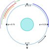 |
Fig. 1 Schematic representation of the orbit of KELT-9 b to scale, with the orbital phases covered in this study colour-coded according to observing night (Blue: HARPS-N N1; Orange: HARPS-N N2; Purple: HARPS-N N3; Red: CARMENES N1; Green: CARMENES N2). The exoplanet orbits counterclockwise (curved arrow), and the observer is positioned at the bottom of the figure. |
2.2.1 Night selection
Our goal for this study is to obtain the most complete phase coverage between quadratures (orbital phases 0.25 < φ < 0.75), while at the same time minimising the size of the dataset in order to keep it computationally feasible to run Markov-chain Monte Carlo sampling on the data. We note that the secondary eclipse of KELT-9b occurs between orbital phases 0.44 < φ < 0.56, and the spectra falling within this interval were excluded from the analysis. Overall, we combined three nights of proprietary HARPS-N (Cosentino et al. 2012; R = 115 000, spectral coverage 390–690 nm) data1 with two nights of public CARMENES (Quirrenbach et al. 2016, 2018; R ~ 94 600, spectral coverage 520–960 nm in the optical arm) data2. We define our naming convention for the observing nights and list relevant parameters in Table 1. We visualise the orbital phases covered in Fig. 1. We only used the optical arm of CARMENES, where we expect most of the Fe I signal to arise.
The HARPS-N nights were obtained within a Large Program (PI: Micela) awarded to the GAPS Collaboration (Poretti et al. 2016). This program has already yielded results on atmospheric characterisation (e.g. Borsa et al. 2019; Pino et al. 2020; Guilluy et al. 2020; Rainer et al. 2021; Scandariato et al. 2021) and is described in Guilluy et al. (2022). We initially included the HARPS-N night published in Pino et al. (2020), covering phases pre-secondary eclipse, and a second HARPS-N night post-secondary eclipse observed at lower S/N. To compensate for the latter, we added the two best archival nights of CARMENES post-secondary eclipse. While performing the analysis, we observed a third HARPS-N night, also post-secondary eclipse, which we integrated into the analysis to test for consistency between different instruments and observing dates.
The two CARMENES nights included spectra at very low S/N and very high airmass. Four spectra at visibly low S/N between phase 0.55 and 0.60 were removed from the night of 2018 September 2. To this end, a threshold of 35% of the maximum median S/N calculated across all wavelengths was applied. Furthermore, we excluded spectra taken at airmass greater than 1.8 from the analysis. With this choice, we minimised the size of the confidence intervals on the retrieved planetary orbital velocity. However, the exact choice of the airmass threshold does not significantly affect the combined analysis. Finally, we removed the ten reddest orders of CARMENES from the analysis due to very low S/N.
At the unusually high level of precision that we obtain for radial velocity, it is important to account for the fact that the time-stamps stored in the headers of both CARMENES and HARPS-N spectra for our planet contain BJD dates computed in the UTC frame rather than in the TDB frame. Indeed, between 2017 and 2021 inclusive, the difference BJD UTC – BJD TDB is fixed and amounts to 69.2 s, which is non-negligible for us. All the dates in the file headers are correctly weighted by the photometric barycentre of the exposure, that is, they account for the fact that varying flux during the exposure can effectively offset the point where half of the flux is collected from the middle of the exposure.
All in all, our full set of data consists of 320 spectra covering orbital phases φ = 0.233–0.772 and excluding the secondary eclipse as mentioned above. While the reliance on just one HARPS-N night pre-secondary eclipse might seem unbalanced, the exceptionally high quality of the pre-secondary eclipse HARPS-N night results in similar confidence intervals to those obtained when the pre-secondary eclipse and the post-secondary eclipse phases are analysed separately.
Details of the five observing nights included in this study.
2.2.2 Data reduction
We designed a pipeline that we can uniformly apply to HARPS-N and CARMENES. Both HARPS-N (we used the e2ds spectra) and CARMENES spectra are provided with a wavelength solution in the rest frame of the observer, in air for HARPS-N and in vacuum for CARMENES. We shift the HARPS-N wavelength solution to vacuum to be able to compare them with models. After deblazing and colour-correcting the spectra, we proceeded to shift them into the barycentric reference frame of the Solar System by applying the barycentric correction included in the respective file headers. We followed the work of Pino et al. (2020) for this part of the analysis.
We then applied a telluric and stellar line correction adapted from Giacobbe et al. (2021) and originally designed to clean near-infrared data from the more severe effects of telluric and instrumental systematic effects. This procedure consists in the application of a principal component analysis (PCA) algorithm to blindly identify ‘state vectors’ in common between spectral channels and use them to describe the time-evolution of telluric lines and remove them. We work in the barycentric rest frame, where stellar lines are stationary and telluric lines are quasi-stationary. In this way, we slightly privilege the correction of stellar lines over telluric lines, although in reality the algorithm removes both components. This choice is driven by our focus on neutral iron lines, which are typically present in both stellar and planetary spectra, but not in the Earth’s atmosphere. As there are some differences between the algorithm of Giacobbe et al. (2021) and that used in this work, we fully describe our implementation of the PCA. We note that, in the exoplanet literature, PCA is sometimes performed by only using the singular value decomposition (SVD) algorithm, while in our case SVD is just one of three main steps of the analysis. While conceptually very similar, the full PCA algorithm described here and the SVD-only algorithm differ in the way the wavelength channels in the data are weighted.
We describe the data as a cube with three axes: order number, time (or phase), and wavelength. One cube is stored for each night of observations. Due to the fixed layout of the echellogram for both CARMENES and HARPS-N, the dimension along the order axis is always 61 for CARMENES and 69 for HARPS-N. The corresponding number of pixels along the wavelength dimension is 4096 for both spectrographs.
The PCA algorithm in this analysis is entirely written in Python and based on NumPy methods. The code is run on each night and each order separately, recognising not only that the atmosphere behaves differently on each night, but also that different orders are affected by different time-correlated sources, both astrophysical and instrumental. The input matrix for the algorithm is always a 2D array, with time on the vertical axis (along a column) and wavelength on the horizontal axis (along a row).
The PCA algorithm, applied independently to each spectral order and each observing night, is outlined as follows:
Initial masking: non-finite flux values (NaN) and values below 2% of the median flux level (low-S/N) of the spectrum are flagged and a mask is created to keep track of such pixels. Spectral channels (data columns) with more than one invalid pixel are entirely masked.
Standardisation: each column (each spectral channel) has its mean subtracted and is divided by its standard deviation. At the end of the process, each column therefore has zero mean and unit standard deviation. This step makes sure that the PCA weights all wavelength bins equally while looking for common modes in the next step.
SVD: this is computed via numpy.linalg.svd() on the standardised matrix (step 2), with the option full_matrices = False. SVD decomposes the array in a set of orthogonal eigenvectors and corresponding eigenvalues. In our case, there are as many eigenvectors(values) as there are spectral channels, and their number corresponds to the dimension of the wavelength axis. In PCA nomenclature, this choice corresponds to running the PCA in the ‘time domain’, that is, with time (or orbital phase) as an independent variable. We note that we only feed the SVD algorithm the columns of data that were not masked at step 1.
Component selection: SVD ranks eigenvectors according to their contribution to the data variance. Therefore, only the first few eigenvectors are needed to describe most of the flux variations in telluric lines. In our case, by visual inspection, we determined that two eigenvectors (also referred to as components) are sufficient to suppress telluric lines below the level of the noise for all the spectral orders, and we use those in the following step.
Multilinear regression: the eigenvalues obtained via SVD do not correctly describe the observed data, because they have been computed on the standardised flux array (step 2) rather than on the measured flux array (step 1). Therefore, we run a multi-linear regression (MLR) between the set of two eigenvectors v1(t), v2(t) determined at step 4 and the matrix stored at step 1. For each spectral channel i in the matrix, the MLR calculates two eigenvalues c1i, c2i plus an offset c0i.
For each spectral channel i, we calculate the linear combination li(t) = c0i + c1iv1(t) + c2iv2(t) and divide the corresponding column of the matrix at point 1 through it, obtaining a residual matrix.
High-pass filtering: columns in the residual matrix (step 6) that deviate by more than three times the standard deviation of the whole matrix are masked. This mask is then merged via boolean OR with the mask at step 1, and stored for future use during model reprocessing (Sect. 2.3). Low-order variations in each spectrum, that is, along the wavelength axis, are fitted with a second-order polynomial (excluding the masked pixels) and divided out.
The mean of each spectrum obtained in step 7 is subtracted out, which is necessary to compute the log-likelihood function. We note that the mean is calculated by excluding the masked pixels; these are then manually reset to zero so that they do not contribute to the log-likelihood function.
The five resulting data cubes (one per observing night) are then compared to models.
2.3 Models
We produced a set of nested models to test the presence of 3D effects in the atmosphere of KELT-9b, generalising the best-fit 1D model by Pino et al. (2020). This is calculated employing a custom line-by-line radiative transfer code, which solves the radiative transfer equation in its integral form using a ‘linear in optical depth approximation’ for the source function (Toon et al. 1989). Here, the temperature-pressure profile calculated by Lothringer et al. (2018) is assumed. Volume mixing ratios are calculated under the assumption of equilibrium chemistry using FastChem version 2 (Stock et al. 2018), with stellar (solar in the case of KELT-9) composition. Following Pino et al. (2020), we only include lines from neutral iron, whose opacities we compute starting from the VALD3 database (Piskunov et al. 1995; Ryabchikova et al. 1997, 2015; Kupka et al. 1999, 2000)3, and the bound-free H− opacity from John (1988). We convolve the model with two kernels: the former is a Gaussian kernel with FWHM matching the velocity resolution of the HARPS-N/CARMENES spectrographs; the latter is a rotational kernel calculated assuming a rigidly rotating planet with an equatorial velocity of 6.64 km s−1. This value is obtained by assuming synchronous rotation and the planet radius from Gaudi et al. (2017). We refer to Pino et al. (2020) for other details about the radiative transfer code.
Our one-dimensional fiducial model 1C is built using the best-fit spectrum by Pino et al. (2020) as a template, and is described by three parameters: Kp, vsys, and S. The parameter S is a multiplicative scaling factor that accounts for a mismatch between the intensity of model lines and lines in observations (Brogi & Line 2019). With no additional contribution to Doppler shift (e.g. atmospheric winds), the parameters Kp and vsys are physically interpreted as, respectively, the maximum Keplerian orbital velocity of the planet (assuming a circular orbit in the case of model 1C) and the systemic velocity of the system, that is, the constant component of the radial velocity of the system’s centre of mass relative to the Solar System barycentre, which may also include an instrument-dependent radial velocity offset (Deeg & Belmonte 2018). We keep nomenclature consistent with the literature, but caution the reader that additional velocity contributions present in the data will be captured by this model, changing the physical interpretation of these parameters (e.g. see Sect. 4.3). The same caveat applies to the following models.
Model 1C contains limited information about the phase-dependence of the planet spectrum. Indeed, the model has a constant shape across phases, and has a varying Doppler shift with planetary phase that is forced to follow a Keplerian, circular orbit around the system centre of mass. This model has been used by Pino et al. (2020), who show that it accurately reproduces the average Fe I emission line of the planet in HARPS-N N1. We generalise this model by relaxing two separate assumptions: firstly, that the rest frame from which the signal arises is revolving around the star KELT-9 with a circular motion; and secondly, that the flux emitted from the photosphere of the planet is uniform with longitude. Table 2 summarises the models and their parameters, and in the following we describe them more in detail.
We designed an eccentric orbit model 1E for KELT-9b using the parameters  and
and  , where e is the eccentricity, and ω is the argument of periastron. This parameterization performs as fast as or faster than alternatives in an MCMC, and in addition is free of the burden of dealing with angular parameters. Finally, it naturally sets a uniform prior in e and ω that is regarded as the most sensible choice for hot Jupiters (Eastman et al. 2013). This model is described by five parameters: Kp, vsys, and S, which are the same as for the circular orbit model 1C, and h and k in addition.
Finally, we employ two simple modelling approaches to capture the possible variation in intensity of the iron lines as a function of longitude in the planet atmosphere. In both approaches, we neglect latitudinal variations of atmospheric properties, and therefore properties measured at a given longitude should be seen as a latitudinal average. In the first approach, the two four-scaling factor models 4C (circular orbit) and 4E (eccentric orbit) divide the orbital range into four parts (0.25 < φ < 0.35, 0.35 < φ < 0.45, 0.55 < φ < 0.65, and 0.65 < φ < 0.75). We assign a different scaling factor (S1, S2, S3, S4) to each of these phase ranges, while they all share the same orbital parameters (Kp, vsys, and additionally h and k in the case of an eccentric orbit). With this choice, our models are able to capture an inhomogeneous intensity of Fe I lines. For instance, if the Fe I signal mostly comes from the planet dayside, S1 and S4 should be smaller than S2 and S3, because a larger portion of the nightside contributes to determining them. The shortcoming of this modelling approach is that it mixes information coming from different longitudinal slices of the planet atmosphere in a suboptimal way. Indeed, a given longitudinal slice of the planet atmosphere could be observable in multiple phase ranges. The second modelling approach that we consider in this work overcomes this limitation. We adopt three models based on reflection off a Lambert sphere (Collier Cameron et al. 2002). While this is likely unrealistic, we argue that these models have the desirable feature that line intensity has a maximum (whose position is a parameter model Loff) and then decreases symmetrically when moving further away in longitude. This would, for instance, reproduce a shallower thermal gradient profile, or a decrease in neutral iron abundance while moving towards the nightside. In this model, we substitute the constant multiplicative scaling factor S with the phase function g(φ):
![Mathematical equation: $g\left( \varphi \right) = {S \over \pi } + {{{S_{{\rm{Lambert}}}}\,\cdot\,\left[ {\sin \alpha + \left( {\pi - \alpha } \right)\,\cdot\,\cos \alpha } \right]} \over \pi },$](/articles/aa/full_html/2022/12/aa44593-22/aa44593-22-eq8.png) (2)
(2)
 (3)
(3)
where we assume a perfectly edge-on orbit and φ varies between 0 (inferior conjunction) and 1. In model Lbase, the free parameters are Kp, vsys, S (constant scaling factor contributing emission independent of planetary phase), SLambert (scaling factor of additional phase-dependent Fe I line emission), h and k, and we fix φ0 = 0 (offset of the maximum scaling factor from the substellar point). We additionally test model L where we also suppress the phase-independent emission (S = 0, φ = 0).
All our models rely on several simplifying assumptions, and adopt a parameterized approach that is agnostic of the underlying physics. In future work, we will consider more physically motivated parameterized models able to partially account for the interplay between stellar irradiation, atmospheric dynamics, and structure, and thus predict variations in thermal profile and chemistry as a function of longitude (e.g. Dobbs-Dixon & Blecic 2022).
Model description, parameters, and priors.
2.4 Cross-correlation-likelihood mapping
Pino et al. (2020) used two different methods to stack the signal from thousands of iron lines, yielding the first detection of iron in the emission spectrum of KELT-9b: (1) a weighted mask method, and (2) a cross-correlation-likelihood mapping scheme by Brogi & Line (2019). In this paper, we employ the cross-correlation-likelihood mapping method, and provide our rationale for this choice in Appendix A. We stress that each method has strengths and weaknesses, and the choice should be driven by the science goals.
The mapping is achieved through the use of the log-likelihood function
 (4)
(4)
where N is the number of valid (i.e. unmasked) spectral channels on each spectrum and each order,  and
and  are the data and model variances, respectively, and R is the cross-covariance between model and data. While cross-correlation does not appear explicitly in this formula, its numerator (R) and denominator (sfsg) are present in the argument of the natural logarithm. We partition Eq. (4) by calculating it on each order and frame. This correctly weights for noise variations – that are directly estimated from the sample variance – across orders and frames. This methodology has been shown to produce unbiased and accurate results (Brogi & Line 2019; Gibson et al. 2022).
As pointed out since the early application of the log-likelihood framework (Brogi & Line 2019; Pino et al. 2020; Gibson et al. 2020), the model spectrum cannot be compared to the data directly, that is, simply by scaling and shifting it. In order to avoid biases in the retrieved parameters, it is important to reproduce on the model any possible alteration of the planet signal induced by the data reduction process. This is achieved by running a parallel data analysis chain (steps 1-6 in Sect. 2.2.2) on a data cube where the model is injected on top of the observed data at a reduced amplitude of 1%4, so that the injection does not alter the analysis, in particular the ranking of the SVD components at step 3. Each injected spectrum Finj is obtained from the observed spectrum Fobs via
 (5)
(5)
where θ is the state vector containing all the model parameters at the current MCMC step, and the model is expressed in planet or star units by normalising through a stellar black body at the effective temperature of KELT-9.
After step 6 of the analysis, the observed dataset at the same stage is subtracted out, so that the resulting data cube represents the (noiseless) processed model. The latter is then multiplied by 100 to restore its original amplitude; is mean-subtracted as in step 8; and is then used to calculate the log-likelihood values through Eq. (4) after masking (i.e. setting to zero) the same pixels as for the observed data. We skip the application of a high-pass filter (step 7) on the model. While early tests indicate no impact on the final results, we believe that application of the filter on observed data (dominated by instrumental and photon noise) is conceptually different from application on the noiseless model (dominated by signal variations). We additionally note that, except for a constant offset of 1, subtracting or dividing through the PCA-processed data after step 6 of the analysis leads to differences within a factor of order (Fpl/F*)2, that is a difference of the order of 10−8 in absolute flux (or 10−4 in relative flux). Here we opt for subtracting to avoid possible issues with division by values close to zero.
The difference between the model injected at step 1 and the model processed as above is shown in Fig. 2. This comparison shows how even by visual inspection there are evident alterations in the depth and shape of the planetary lines that need to be accounted for. As expected, the effect is phase-dependent and particularly severe close to quadrature, where the planet trail is nearly parallel to telluric and stellar lines. In Appendix B, we show that our reprocessing methodology is capable of recovering a phase-dependent signal accurately at our level of precision.
Currently, model reprocessing is the bottleneck of our retrieval code. In order to optimise this part of the code, we follow the practice of Gibson et al. (2022) and for model reprocessing we reuse the same eigenvectors calculated by the SVD algorithm on the observed spectra (step 3). We also reuse the same mask for both analysis and reprocessing. With these choices, we speed up the calculation by a factor of about 2.
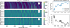 |
Fig. 2 Effects of telluric removal on the signal from KELT-9 b. Left: best-fit Fe I emission model Doppler-shifted based on the orbital parameters of KELT-9 b (panel a), injected on top of the first night of HARPS-N data, and passed through the analysis described in Sect. 2.2.2. The signal is recovered with evident alterations, as shown in the reference frame of the observer (panel b) and in the planet’s rest frame (panel c). Top-right: recovered amplitude of a strong injected Fe line as a function of orbital phase (solid) versus its amplitude at injection (dashed). Bottom-right: percent loss of the Fe signal due to the telluric-removal analysis. Nearly 100% of the signal is lost around quadrature. |
3 Results
3.1 Confirmation of iron emission lines from the dayside of KELT-9b
We ran an MCMC using model 1C, the same model that was adopted by Pino et al. (2020), on each individual night. We detect neutral iron in each of the unpublished HARPS-N N2 and N3, and in each of the two CARMENES N1 and N2. This confirms the results of Pino et al. (2020) and Kasper et al. (2021) based on pre-eclipse observations, and shows that neutral iron is also present at post-eclipse phases. Our best single-night detection is still HARPS-N N1, which featured better observing conditions and twice the exposures compared to HARPS-N N2. In HARPS-N Nl, we measure a Kp that is incompatible at 1σ with Pino et al. (2020), despite using the same data. This discrepancy is due to the different ephemeris adopted in this work (see Sect. 2.1). We directly verified that our new PCA pipeline, when applied using the same ephemeris adopted by Pino et al. (2020), reproduces their best-fit planetary orbital velocities. HARPS-N N3 features a similar total S/N compared to HARPS-N Nl, but provides looser constraints on vsys and Kp, and a marginally lower scaling factor. Furthermore, CARMENES provides looser confidence intervals on the parameters compared to HARPS-N. For comparison, the precision reached on all parameters in the best of the two CARMENES nights (CARMENES Nl) is comparable to the precision reached in the worst HARPS-N night (HARPS-N N2).
It is not immediately clear why HARPS-N outperforms CARMENES in our analysis, and multiple factors could be at play. Firstly, the S/N estimates for the CARMENES and HARPS-N datasets are provided by the respective pipelines, and are therefore not necessarily comparable. A proper assessment of the S/Ns would require us to homogeneously reduce the raw frames of both instruments, which is out of the scope of this paper. Second, the amount of signal intrinsically carried in different wavelength ranges could differ, because of the differences in strength and number of Fe I lines and planet-to-star flux ratio. In Appendix C we show that bluer wavelengths (probed by HARPS-N) seem to carry more information about Fe I compared to redder wavelengths (probed by CARMENES) in KELT-9b. Finally, telluric correction is more severe at the redder wavelengths probed by CARMENES. We cannot exclude that, if present, the cumulative effect of slight telluric residuals left behind by our analysis, despite being buried in the photon noise, would more likely negatively impact the CARMENES observations.
Most of the individual posteriors are compatible with each other at 1σ (see Fig. 3 and Appendix D). The only exceptions are: the posteriors for the scaling factor in HARPS-N N2 (orange posterior) and HARPS-N N3 (purple posterior), which are marginally incompatible with each other; and the posterior for Kp in HARPS-N Nl (blue posterior), which is only compatible with HARPS-N N2 (orange posterior). As the discrepancy in the posteriors for the scaling factor between HARPS-N N2 and HARPS-N N3 (orange and purple posterior) is little more than 2σ, we do not consider it significant. We therefore refrain from interpreting it as an astrophysical signal, given also the significant impact of the PCA on the strengths of Fe I lines (see Fig. 2), which needs to be very accurately captured by our injection method for a correct interpretation. However, we note that HARPS-N N3 was observed at least two years after the other epochs, meaning that any variability in the planet atmosphere on year-long timescales would be visible. In addition, we observe a discrepancy in Kp that concerns the only pre-eclipse night that we observed. We consider this discrepancy more likely real, and possibly indicative of a pre-eclipse–post-eclipse asymmetry. We exclude that this is caused by the nodal precession of KELT-9b (Stephan et al. 2022), which would only change the inclination of the orbit by about 1° in three years and whose effect on Kp would be at the 10−4 level. We return to our interpretation of the variation of Kp in the following section and in Sect. 4.3.
We also performed a combined analysis of the nights. The combined analysis leads to a marked improvement in the precision of each parameter (the relative corner plot is displayed in Fig. 4). Our best-fit parameters are  km s−1,
  km s−1 and
  (see Table F.1). Similarly to Pino et al. (2020), we find that our model underpredicts the Fe I line intensity by a factor of about 2. This could be due to an underestimation of the temperature of the upper atmosphere (e.g. Fossati et al. 2020, 2021), an underestimation of the Fe I volume mixing ratio, an overestimation of the stellar flux, the presence of other atomic and molecular species in the spectrum that partially mask neutral iron spectral features (Kasper et al. 2021), or a combination of these. Understanding the source of this discrepancy is out of the scope of this paper, and our conclusions do not hinge on exactly reproducing the Fe I line depth with our 1D model template.
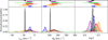 |
Fig. 3 Posterior distributions of parameters of model 1C fit with an MCMC to HARPS-N N1 (blue), HARPS-N N2 (orange), CARMENES N1 (red), CARMENES N2 (green), HARPS-N N3 (purple), and all five nights combined (black). Lower panels: normalised posteriors (higher peak for better constrained parameters), and the marked improvement obtained when combining all data sets. Upper panels: 1σ (dark colour) and 2σ (light colour) confidence intervals obtained from the corresponding posteriors in the lower panels. |
3.2 Neutral iron lines trace a displacement from a circular orbit for KELT-9b
Encouraged by the sub-kilometre-per-second precision reached on five combined nights with model 1C, we perform a fit using an eccentric orbit (model 1E, see Table 2). We obtained bound posteriors for all parameters of model 1E, and converted the posteriors in h and k to posteriors in e and ω by converting every MCMC sample of h and k using e = h2 + k2 and ω = arctan (h/k), and building the corresponding probability distribution. We show the posteriors in Fig. 4, and our best-fit parameters are:  km s−1,
  km s−1,
  ,
,  , and
, and  (see Table F.1).
This result is surprising at face value and is in apparent contrast with the findings of Wong et al. (2020). Indeed, these authors report a tight upper limit to the eccentricity of the planet of e < 0.007 at 2σ using TESS photometry, and additionally find that the addition of parameters e and ω is disfavoured by Bayesian information criterion (BIC) and Akaike information criterion (AIC) in their analysis, indicating a likely circular orbit, as is expected for KELT-9b. In Sects. 4.2 and 4.3 we reconcile our result with that of Wong et al. (2020) by interpreting our measured eccentricity as apparent, and as being due to atmospheric dynamics (winds). For now, we simply note that model 1E captures a significant deviation from a circular orbit traced by Fe I lines, independently of the source of the anomaly.
As model 1E has additional parameters compared to model 1C, we performed a model comparison to determine whether the additional complexity is justified by the data, using several methods: likelihood ratio test, AIC, and BIC. As models 1C and 1E are nested, we applied the likelihood ratio test (as described in Appendix D in Pino et al. 2020) with two fixed parameters and obtain a 5σ preference for the eccentric model. We also obtain the apparently contrasting results that the BIC test strongly favours the circular orbit solution (BIC1E – BIC1C = 7.9), while AIC strongly favours the eccentric orbit solution (AIC1E − AIC1C = −24.5) with a 4.5σ preference, where preference is calculated from the relative likelihood of model 1C exp(AIC1E − AIC1C)/2 converted to σ level using a two-tailed normal distribution test5. In reality, this is not surprising: the BIC test penalises higher complexity models much more than the AIC test, and this difference is more marked for larger data sets. We fit ntot = 71 978 272 pixels simultaneously. Thus, for a change in the number of parameters of 2, the penalty term in the BIC test is 2 log(ntot) = 36.2, compared to 4 for the AIC test. In other words, the BIC test is much more demanding in terms of quality of fit for higher complexity models.
We now compare the posterior distributions for models 1C and 1E (see Fig. 4). Eccentricity and argument of periastron are partially degenerate with Kp. As a result, the marginalised distribution for Kp is slightly broader in model 1E. All common parameters between models 1C and 1E are compatible at 2σ. The eccentricity that we measure has a significance of more than 5σ, which, in combination with the AIC test, suggests that model IE better explains the data compared to model 1C, and that the addition of parameters describing an eccentric orbit is justified.
We developed a new method to display the radial velocity displacement from the best-fit rest frame of the planet (∆vrest) as a function of planet phase (planet trail) in the context of the likelihood framework by Brogi & Line (2019). Conceptually, we can build the planet trail for a given solution as the conditional probability of ∆vrest at every planetary phase, given the best-fit values for the model considered. We use conditional probability and not marginal probability, since we are interested in the value of ∆vrest for the given best-fit solution, rather than in identifying the most likely values of ∆vrest independently of the other parameters. In this representation, the confidence interval obtained at every phase is completely independent of all other phases, and confidence intervals of adjacent phases are not related. Practically, we divide the covered phase range in 0.02-wide phase bins, and for each phase bin we calculate the conditional likelihood as:
 (6)
(6)
where each phase bin is sampled by n exposures (n could differ in every phase bin), the subscript BF indicates the best-fit value for a parameter, and h and k appear as additional parameters evaluated in the best-fit position in the eccentric orbit case. The assumptions behind Eq. (6) are that there is no atmospheric variability, and that each phase bin is small enough that we can neglect the planet motion within it. Finally, in every bin, we calculate the 1σ and 2σ deviations from the maximum likelihood in Δvrest using Wilk’s theorem. Figure 5 displays the resulting trail in the best-fit planetary rest frame using a box plot (Hyndman 1996) for models 1C and 1E. Multi-peaked solutions likely correspond to phase bins where the best-fit solution is not very well constrained, meaning that 1σ and 2σ deviations capture additional spurious peaks. In the eccentric orbit case, the trail appears as a vertical line (except for a few noisy phase bins), which is the expectation in the case that we are in the rest frame from which the lines originate. On the contrary, in the circular orbit case, the trail appears slanted. This indicates that a circular orbit is not fully capable of capturing the morphology of the planet trail, or in other words that the rest frame from which the neutral iron signal is generated deviates from a circular orbit.
In conclusion, our results markedly favour model 1E over model 1C, indicating the presence of a significant radial velocity anomaly detected for Fe I lines. As mentioned above, and further addressed in Sects. 4.2 and 4.3, such a radial velocity anomaly is unlikely to be due to the orbital motion of the planet, and is more likely the result of atmospheric dynamics in KELT-9b.
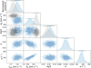 |
Fig. 4 Posterior for the MCMC fit of models 1C (circular orbit, black histograms) and 1E (eccentric orbit, blue histograms). The 1σ and 2σ confidence intervals are indicated with darker and lighter shades, respectively. |
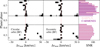 |
Fig. 5 Time-resolved confidence intervals as a function of the planet rest-frame velocity obtained by binning (i.e. co-adding) the individual likelihood functions by 0.02 in orbital phase. Black represents 1σ deviations from the best-fit rest-frame velocity in each phase bin, and grey represents 2σ deviations. The left and centre panels show results for the 1C (circular) and 1E (eccentric) models, respectively, when fixing all the model parameters at their best-fit value, i.e. the median of the posterior distribution. Horizontal black dashed lines indicate phases corresponding to ingress and egress, and a vertical red dashed line indicates the best-fit planet rest-frame. The right panel represents the total S/N achieved within each phase bin, with HARPS-N (lighter pink) and CARMENES (darker purple). |
3.3 Symmetric intensity of iron lines around secondary eclipse
We then searched for variations in the intensity of the observed neutral iron lines while the planet orbits around its host. First, we assumed a circular orbit and fit a separate scaling factor for four mutually exclusive ranges in phase (model 4C). The left panel of Fig. 6 shows the resulting posteriors for the scaling factors. We show the full corner plots in Appendix E (Fig. E.1), and report best-fit parameters and their errors in Table F.1. The MCMC finds well-constrained posteriors for all parameters, indicating that our data contain sufficient information to perform this kind of study. The posteriors of Kp and vsys are in good agreement with those for model 1C. We attribute this to the fact that the scaling factor (hence, neutral iron line intensity) and the orbital parameters (hence, neutral iron line Doppler shift) are not correlated at our level of precision.
We additionally repeated the fit using model 4E, thus allowing for an eccentric orbit. We obtained bound posteriors for all parameters, and compare the resulting scaling factors in the right panel of Fig. 6. We also show full corner plots in Fig. E.2, and report best-fit parameters and their errors in Table F.1. We observe that the scaling factors are uncorrelated with all other parameters at our level of precision. As a result, the posteriors of the phase-resolved scaling factors are very similar to those of model 4C, and the posteriors of orbital parameters are close to those of model IE. We conclude that, at our level of precision, the Doppler-shift and line shape of the exoplanet atmosphere spectra can be modelled separately without any loss of information.
Finally, we ran MCMC chains using Lambert sphere models (L, Loff, Lbase). We achieve convergence on all parameters in these models, and we report the full posteriors in the Appendix (Figs. E.3 and E.4), and best-fit parameters with their errors in Table F.l. The orbital properties (Kp, vsys, e, ω) are in excellent agreement across the three models, confirming that Doppler and line-intensity information are uncorrelated, and confirming the preference for an eccentric orbit.
We compare results from these models and results from model IE and 4E in Fig. 7. A first clear result is that the peak of the emission is tightly constrained at the substellar point. This is supported by the posterior of the parameter φ0 in model Loff, whose value is φ = 0.00 ± 0.01, which translates to an angular displacement from the substellar point of 0 ± 5°. Secondly, model Lbase presents a degeneracy between SLambert and S. In other words, it is possible to explain the data with an intensity profile that decreases moving towards the nightside (akin to model L, where the contribution from the anti-stellar point is forced to 0), but also with a constant intensity profile independent of phase. Solutions with no SLambert contribution are also allowed, while the model supports, at >2<τ significance, the presence of a phase-independent contribution to emission. When comparing the intensity profiles (see Fig. 7), it is clear that both models L and Lbase agree in the range probed by observations (phases 0.25 < φ < 0.45 and 0.55 < φ < 0.75). In addition, all Lambert sphere models are in good agreement with the scaling factors measured with model 4E in the probed planet phase range. We conclude that our data are not sufficient to provide strong evidence of a variation of the intensity of iron lines with longitude. This is further confirmed by the strong preference of model IE over model L and Loff (e.g. AICL − AIC1E = 8.5, and same difference in BIC), and the marginal to strong preference over Lbase according to AIC and BIC ( ; BICLbase − BIC1E = 18). We argue that Lbase is less disfavoured because it allows solutions with smaller to no dependence of the scaling factor on orbital phase, further supporting our results.
On the other hand, we can confidently conclude that there is no detectable asymmetry (e.g. due to a hot-spot offset) in the intensity of lines in pre- and post-eclipse spectra. Indeed, model Loff is strongly disfavoured in terms of BIC and AIC compared to model L (by 19 and 3, respectively), and its parameter φ0 presents a tight posterior around 0.
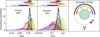 |
Fig. 6 Posterior distribution for the scaling factors of models 1C and 4C (left panel), and IE and 4E (middle panel). Right panel: colour-coded phase ranges corresponding to each of the five parameters for each panel. |
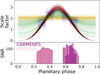 |
Fig. 7 Results of our search for variations in the intensity of the observed neutral iron lines. Upper panel: 100 draws from the posterior for scaling factors as a function of phase obtained by fitting models IE (orange), 4E (blue), L (black), Loff (red) and Lbase (green) to the data. The phase coverage of the data is shown in the lower panel, in terms of the S/N of stellar spectra in each phase bin (HARPS-N: lighter pink; CARMENES: darker purple). Where multiple nights cover the same orbital phase bin, their contributions are summed in quadrature. |
4 Discussion
4.1 HRS phase curves as a new tool for exoplanet atmosphere characterization
Our results show that HRS emission spectroscopy observations of hot gas giants have the potential to reveal much more information when treated as a phase curve rather than a single phase-collapsed emission spectrum, which is the approach that has most often been taken in the literature so far (e.g. Pino et al. 2020; Yan et al. 2020; Nugroho et al. 2020; Borsa et al. 2022). Conceptually, an HRS phase curve is similar to a classic low-resolution (LRS) phase curve observed from space (e.g. Stevenson 2016). The key difference between LRS and HRS phase curves is the observable they record. For LRS phase curves, this is simply the flux of the planet-plus-star system as a function of planetary phase. On the other hand, HRS phase curves record two separate observable quantities.
The first observable quantity is the contrast of planet lines relative to the continuum generated by the star and planet as a function of phase (Pino et al. 2020; also noted and exploited by Herman et al. 2022 and van Sluijs et al. 2022). Unlike in LRS phase curves, the spectral features of the planet continuum are lost because it is impossible to reconstruct the chromatic fibre losses, which are due to differential refraction from Earth atmosphere. Such losses introduce an additional, unknown wavelength and time dependence, which need to be removed from the spectra in order to correct the stellar and telluric lines and extract the planetary signal (e.g. Appendix A of Pino et al. 2020). This is typically performed with a normalisation, which unfortunately also removes the exoplanet atmosphere continuum features. This may seem a strong limitation compared to LRS phase curves, but when interpreted in an appropriate statistical framework (Brogi & Line 2019), HRS emission spectra still contain enough information to constrain the thermal profiles and the volume mixing ratios (Pino et al. 2020; Kasper et al. 2021), including their absolute values (Line et al. 2021). This extends to HRS phase curves. Indeed, both this work and Herman et al. (2022) and van Sluijs et al. (2022) use HRS phase curves to constrain the value of a scaling factor as a function of phase, which is a proxy for the steepness of the thermal gradient and volume mixing ratio of the species present in the cross-correlation template. In addition, compared to LRS phase curves, HRS phase curves probe higher up in the atmosphere, and, thanks to the simultaneous detection of lines of different strengths, a broader span of pressures.
The second observable quantity is the phase-resolved Doppler shift of planet lines. This is obtained by individually resolving the spectral lines (see Sect. 3.2), and is only possible with HRS spectrographs. Herman et al. (2022) do not include this aspect in their analysis, and van Sluijs et al. (2022) indicate that this information is washed out at a resolution of 15 000. At the price of lower efficiency compared to lower resolution slit spectrographs, fibre-fed R ~ 100 000 spectrographs open a new window onto planetary climate and dynamics, which cannot be studied in this way with any other technique (Kawahara 2012; see Sects. 4.2 and 4.3).
Line contrasts and wind-induced Doppler shifts are determined by the complex interplay between energy transport, chemistry, and dynamics, and are therefore intrinsically linked. An appropriate framework to interpret HRS phase curves needs to be able to reproduce both observable quantities simultaneously. This has already been shown by computing HRS spectra starting from the GCMs of irradiated planets (e.g. Zhang et al. 2017; Beltz et al. 2021, 2022a). Unfortunately, such simulations are time-consuming, and using them for data comparison over a large parameter space is currently unrealistic. However, our analysis demonstrates that, to first order, the line contrasts (parameterized by the scaling factor) and the positions (parameterized by Kp, vsys, h, and k) are uncorrelated for KELT-9b. As a result, if Doppler shifts can be attributed to planetary climate, it is possible to build a first-order picture of winds (through line positions) and thermal and/or abundance structure (through line contrasts) even without a GCM analysis (see Sect. 4.3).
4.2 Sensitivity of HRS phase curves to slight eccentricities in UHJs
In Sect. 3.2 we demonstrate that, with our new method based on the relative velocities of the planet probed by its atmospheric emission lines throughout the orbit, HRS phase curves have the potential to detect radial velocity deviations from a circular orbit of the order of a few kilometres per second. In Sect. 3.2, we further demonstrate that, if these deviations were due to a slightly eccentric orbit, they would correspond to a solution of e = 0.016 ± 0.003, which we measured with high significance. In the specific case of KELT-9b, TESS photometry shows that this eccentricity is unlikely to be real (Wong et al. 2020, Sect. 3.2). However, it is interesting to note that, if KELT-9b had an eccentricity of this magnitude, we would have the sensitivity to measure it with our new technique.
The challenge of measuring slight eccentricities of UHJs with traditional methods such as stellar radial velocities and transit photometry is manifold. Indeed, many planets of this class orbit A-type or early F-type stars, which have fast rotational velocities (up to more than 100 km s−1). As a result, the stellar lines are significantly broadened, resulting in reduced stellar radial velocity precision. In addition, at the level of precision required, second-order effects need to be accounted for with detailed models, including for example the radial velocity contamination by tidal bulges induced by the planet on the host star. Transit photometry offers an alternative means by which to measure slight eccentricities, but the interpretation of these measurements is not straightforward. For instance, an inhomogeneous dayside surface brightness of the planet could affect the retrieved mid-occultation timing (Shporer et al. 2014), accurate knowledge of which is necessary to measure a slight eccentricity with this method.
Our method is completely independent, and does not suffer from the same systematic errors as those based on stellar radial velocities and transit photometry. However, as we already discussed in Sect. 3.2 and discuss in more detail in Sect. 4.3, winds of moderate strength (a few kilometres per second) in UHJs can create signals of the same order of magnitude as those induced by a slightly eccentric orbit. Thus, while planetary radial velocities of UHJs could be used to measure or set tight upper limits to the potential slight eccentricities of UHJs, the interpretation of radial velocity anomalies in terms of orbital dynamics or climate could remain challenging.
It is beyond the scope of the present study to explore how such degeneracy can be broken. However, our work already shows that, by combination with independent measurements of eccentricities, our method has the potential to discriminate between the two possibilities. In our case, Wong et al. (2020) provide a tight upper limit by combining information on the timing and duration of the primary and secondary eclipse of KELT-9b (measured by TESS). Indeed, these combined observables depend on the parameters k and h, respectively (Ragozzine & Wolf 2009). Unfortunately, in many practical cases, only the timing difference can be measured to a useful precision, making it impossible to completely determine e and ω (Charbonneau et al. 2005). Still, in the most favourable cases, this method has provided some of the best precision to date on eccentricities, pushing to measuring eccentricities smaller than 0.01 at >5σ significance (e.g. Nymeyer et al. 2011). Extensive stellar radial velocity campaigns have also demonstrated that it is possible to significantly measure eccentricities smaller than 0.01 in the best cases. For example, Bonomo et al. (2017), who present one of the largest homogeneous studies of eccentricities, significantly measured eccentricities smaller than 0.01 in 10 out of 231 planets. However, those cases all correspond to planets orbiting relatively slowly rotating host stars (v sin(i) < 20 km s−1), and are the subject of multi-year radial velocity campaigns, meaning that they still represent a minority.
One more possible means by which we could be able to break this degeneracy is to exploit the different shape of the radial velocity anomaly produced by different wind patterns (see Sect. 4.3), and by an eccentric orbit. Through detailed modelling, and using a wide planetary phase coverage, it could indeed be possible to distinguish between the different cases based on the radial velocity anomaly morphology. For instance, Kawahara (2012) showed that the additional modulation induced by a slightly eccentric orbit over a circular one has half the period of the corresponding circular orbit, while planetary rotation, and by extension simple wind patterns, induce a deviation with a full orbital period (see also Sect. 4.3). Planetary radial velocities obtained towards quadrature and beyond (pushing into the night-side) are likely the most suitable tools with which to disentangle these solutions. We will further explore this idea in future work.
Finally, combining information from multiple species could prove to be key to ultimately breaking this degeneracy. Eccentricity would produce the same radial velocity anomaly independently of the species or specific lines analysed. On the other hand, winds are expected to be altitude dependent. Lines of different oscillator strength probe different altitudes in the atmosphere, spanning several orders of magnitude in pressure with HRS (e.g. Pino et al. 2020). As a result, the radial velocity measured through different subsets of lines or atmospheric species that probe different altitudes would change depending on the wind pattern experienced by them.
Thanks to the advent of new-generation spectrographs mounted on eight-metre class telescopes, which have better throughput and broader spectral coverage (e.g. ESPRESSO@VLT, MAROON-X@Gemini-N), the same precision that we achieve for KELT-9b using Fe I lines only will be reached for systems at least 2.5 mag dimmer than KELT-9b (pushing up to V = 9). Despite the challenges outlined above, the prospect of a survey of eccentricities for this class of planets is tantalising, as it would provide a means to study UHJ evolution history, and potentially their internal structure (Fortney et al. 2021).
4.3 The climate of KELT-9b
As discussed in Sect. 3.2, we consider it unlikely that the orbit of KELT-9b is actually eccentric. To reconcile our results with those of Wong et al. (2020), we therefore explored an alternative and more likely scenario in which the neutral iron signal comes from a localised region of the planet dayside atmosphere. Indeed, in this scenario, this region will show changes in net Doppler shift due to rotation and winds, and the Doppler shift of the neutral iron lines would track them.
We built a toy model to capture this effect. We define two sets of spherical polar coordinate systems to represent a spherical planet: (β, α) represent the latitude and longitude in a reference frame centred in the planet, with the observer located along the x-axis (α = 0); (θ, ϕ) represent the latitude and longitude in a reference frame centred in the planet, co-rotating with the planet and with the substellar point located along the x-axis (ϕ = 0). As KELT-9b is transiting, we assume that the orbital inclination is 90°, which leads to the relations θ = β and α = ϕ + φ, where φ is the planet phase. We assume a solid-body rotation for the planet, and an obliquity of 0°. We additionally allow for a zonal wind flow: we model both an eastward wind and a day-to-night wind, which are the wind circulation patterns largely predicted to be dominant by GCMs of KELT-9b (Komacek et al. 2017). The line-of-sight (LOS) component of the velocity of a mass of iron gas located at coordinates (β, α) is therefore
 (7)
(7)
where Rp is the radius of the planet, Ω is the angular velocity derived from the orbital period, and vwind is always positive in the eastward jet case but is negative (contrary to the sense of planet rotation) for ϕ < π in the day-to-night flow case. In addition, we need to take into account that not every surface element of the planet contributes to the net Doppler shift in the same way. Following Zhang et al. (2017), we weight every contribution by the flux emitted in the direction of the observer. The projection of the normal to the local surface along the direction of observation results in a factor of µ = cos α sinβ, which is the visibility weight. Finally, we weight every surface element with a value of 1 if it is located in the dayside of the planet, and 0 if it is located in the nightside of the planet in order to account for the uneven brightness distribution.
We compare the predictions of this toy model with the planet trail obtained in the best-fit circular orbit rest frame of the planet in Fig. 8. In the case of pure rotation, we can intuitively understand the curve. Immediately after transit (φ = 0), the dayside starts to be visible as it rotates towards the observer. As a result, the net Doppler shift is negative and close in value to the rotational velocity. While more of the blueshifted dayside is visible with increasing planet phase, the Doppler shift becomes dominated by regions of the planet that have a smaller projected velocity component towards the observer due to geometry, and therefore its magnitude decreases. After phase 0.25, part of the visible dayside is rotating away from the observer. At φ = 0.5, the two parts cancel out exactly as the dayside is completely visible. The effect is symmetric for φ > 0.5. The discontinuity at φ = 0 is due to our assumption that the nightside is not contributing to the emission (Beltz et al. 2022a). This reasoning is easily extended to the case of eastward wind, which simply adds to the planet rotation velocity, while the day-to-night flow case is slightly more complicated, but can be understood with similar reasoning.
The pure rotation curve (blue curve) is consistent with the trail at the 2σ level in the majority of the individual phase bins, both in pre-eclipse and post-eclipse. However, it does not seem to correctly capture the trends in either phase range. In the pre-eclipse (φ < 0.5) phase range, the trail appears to be steeper than the prediction made by the pure rotation model. In other words, the rotation alone seems to be too slow to explain the pre-eclipse trail. The addition of zonal flows in the direction of rotation provides a possible solution. In this phase range, the wind flows induced by both an eastward jet (green curve) or a day-to-night circulation pattern (orange curve) are aligned with the planet rotation. We find that with the addition of an eastward wind model with vwind = 10 km s−1, the prediction matches the observed slope of the trail better than that of the pure rotation case. However, this model fails to reproduce the evidence for redshift observed immediately before eclipse, and it deviates from the trail in the post-eclipse range where the trail appears flatter. Both these trends are instead captured by a rotation plus day-to-night flow model with vwind = 5 km s−1. Indeed, in this configuration, the winds tend to redshift the signal close to secondary eclipse, and to counteract the effect of rotation in post-eclipse phases, producing a trail that is nearly constant with phase.
Our results are broadly consistent with expectations from GCMs and Spitzer phase curve observations of KELT-9b. Indeed, Mansfield et al. (2020) indicate a preference for strong drag GCMs to explain the dayside phase curve of this planet. In strong drag models, the drag timescale is short compared to the rotational timescale. As a result, the balance in the horizontal angular momentum is primarily between the drag force (e.g. dissipation due to the interaction between the planetary magnetic field and the ions in the atmosphere) and the day-night thermal forcing. This results in a day-to-night flow that is roughly symmetric around the substellar point (Showman & Polvani 2011; Tan & Komacek 2019). For KELT-9b, GCMs predict wind speeds of about 5 km s−1, a roughly symmetric thermal structure around the substellar point, and a day-to-night flow at the photospheric pressures probed by Spitzer (Tan & Komacek 2019; Mansfield et al. 2020). This is in very good agreement with the results from our HRS phase curve, which shows symmetry in line intensities around the substellar point (Sect. 3.3) and a phase-dependent Doppler shift that is well reproduced by day-to-night wind flows with the speeds predicted by GCMs (this section). In addition, Wong et al. (2020) report a small eastward hot-spot offset of 5.2 ± 0.9°, which is consistent with our upper limit to the scaling factor asymmetry in the HRS phase curve. Indeed, in the presence of a hot-spot offset driven by an eastward super-rotating jet, we could expect the steepness of the thermal gradient and the iron ionisation fraction to vary across the dayside in an asymmetric way, which would be picked by our retrievals as an asymmetry in the scaling factor as a function of longitude (van Sluijs et al. 2022). However, Mansfield et al. (2020) report a larger hot-spot offset of 19 ± 2°. If the vertical gradient in the thermal structure followed the same longitudinal pattern as the photospheric emission from Spitzer, our retrieval should have the precision to detect it. It is anyway important to note that a coherent explanation of the TESS and Spitzer phase curves for this planet based on GCM models is still missing, and that neutral iron lines in this planet probe atmospheric pressures as low as 10−5 bar (Pino et al. 2020), which is significantly lower than the TESS and Spitzer photosphere (10−1–10−2 bar), and well within the region where the double-grey assumption common to many GCMs does not apply (Rauscher & Menou 2012). As a consequence, a dedicated modelling effort to simultaneously fit LRS and HRS phase curves is necessary; we will consider this in future work.
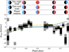 |
Fig. 8 Comparison of planet trail with predictions of radial velocity anomaly induced by rotation and different wind patterns. Lower panel: planetary trail obtained in the best-fit circular orbit reference frame (same as left panel of Fig. 5, but zooming onto smaller radial velocity displacements from the best-fit circular orbit rest frame), and comparison with predictions of net Doppler shift in different cases: pure rotation (blue dashed curve), east-west wind of 10 km s−1 (green dashed curve), and day-to-night wind of 5 km s−1 (orange dot-dashed curve). Upper panel: contribution to Doppler shift from the portion of the planet disk seen at different phases due to the two wind geometries considered and planet rotation. Black portions of the disk correspond to the night-side, while red(blue) portions correspond to regions producing red(blue)shifted lines. Less weight should be given to phase bins close to quadrature (φ < 0.35; φ > 0.65) because of the detrimental effect of our analysis on the S/N in this phase range (see Fig. 2). |
4.4 Implications for wind dynamics measured in transmission spectroscopy
Day-to-night wind flow in KELT-9b was also reported by Pai Asnodkar et al. (2022) and Bello-Arufe et al. (2022) based on the Doppler shift of Fe II lines seen in transmission compared to the stellar systemic velocity. While Fe I traces gas motions in the gravitationally bound part of the atmosphere of a planet, Fe II is likely tracing the dynamics of the evaporating exosphere (Zhang et al. 2022). Therefore, a full analysis combining high-spectral-resolution phase curves and transmission spectroscopy of UHJs has the potential to illuminate the physical processes leading to mass loss in this class of exoplanets. The challenge is that this requires the comparison of different geometries and accurate modelling over a broad range of pressures, possibly including hydrodynamics and non-local thermodynamic equilibrium effects (Huang et al. 2017; Hoeijmakers et al. 2019). This is out of the scope of this paper, and we limit ourselves to a qualitative comparison, and to highlighting potential pathways towards combining the two techniques and related potential caveats.
Both Pai Asnodkar et al. (2022) and Bello-Arufe et al. (2022) report winds directed from dayside to nightside, with speeds of between 5 and 10 km s−1. At a qualitative level, both the wind speed and pattern that they report are consistent with our physical interpretation of the Fe I Doppler shifts emerging from the HRS phase curve. This may suggest that the transition in dynamical regimes is not sharp across the pressures probed by Fe I and Fe II in KELT-9b. At face value, this is surprising, because the two sets of observations likely bridge from the gravitationally bound part of the atmosphere to the exosphere. However, both our analysis and the analyses of Pai Asnodkar et al. (2022) and Bello-Arufe et al. (2022) only account for Doppler shifts of lines, and yet line shapes are also distorted differently by different wind patterns (Seidel et al. 2020). A more detailed analysis that accounts for this effect is therefore necessary in order to properly assess whether or not a transition in the dynamical regime experienced by Fe I and Fe II takes place.
Additionally, Pai Asnodkar et al. (2022) report potential variability in the measured wind speed of several km s−1, although this does not manifest as strong brightness temperature variations for the planet (Jones et al. 2022). We leave the study of the effect of variability to future work, and only note that our observations likely probe deeper layers in the atmosphere, and that our results assume that no variability across our observed epochs is present.
It is also important to note that the measurement of systemic velocity from the stellar lines of KELT-9 appears to be challenging. This highlights a potential weakness of transmission spectra as probes of atmospheric dynamics (Bello-Arufe et al. 2022) in that they rely on the accuracy of the systemic velocity. On the other hand, our measurement only depends on the relative shift of planetary lines during the orbit, and is therefore independent of the value of the systemic velocity. Our result therefore constitutes an independent measurement of the likely presence of day-to-night winds of several kilometre per second blowing at the altitudes probed by neutral atomic species in KELT-9b, which could indeed extend to the upper atmosphere probed by Fe II lines in transmission.
Looking forward, our technique could also be used to revisit results from transmission spectroscopy without using the systemic velocity measured through stellar lines, which is potentially inaccurate at the level of a few km s−1 in this planet (Pino et al. 2020). For instance, our measured value of vsys has a precision of about 0.5 km s−1, which could still be sufficient to compare with Doppler displacements measured in the transmission spectrum of the planet in order to reveal day-to-night winds of several km s−1. However, our measurement is not guaranteed to be a completely accurate estimate of the systemic velocity itself, because it could also partially capture the Doppler shift induced by winds moving neutral iron gas in the atmosphere. Still, vsys values measured assuming a circular or an eccentric orbit (describing winds in our interpretation) are compatible at 1σ (Table D.1). This provides some confidence that our systemic velocity is accurate within 1 km s−1. Our systemic velocity is also consistent with values measured on stellar lines by Pai Asnodkar et al. (2022), Hoeijmakers et al. (2019), and Bello-Arufe et al. (2022), but seems more difficult to reconcile with the value measured by Borsa et al. (2019) and Gaudi et al. (2017), from whose measurements it deviates by 3 and 4 km s−1, respectively. Ultimately, while a more detailed analysis of the potential systematic errors and astrophysical effects impacting the measurement of vsys with each technique is required, our analysis provides additional confidence to the literature estimates of wind speeds measured from transmission spectra in KELT-9b.
4.5 KELT-9b in the context of ultra-hot Jupiters
Our current understanding of the physical processes regulating the climate of hot and ultra-hot gas giants mostly comes from space-borne phase-curve studies. One of the most striking results from these surveys is the relation between day-night temperature contrast, phase offset, and level of stellar irradiation. Phase-curve observations have found a systematic increase in day-night temperature contrast with increasing temperature up to about 2500 K, accompanied by a decrease in hot-spot offset, which is also a prediction of GCMs. More recently, hotter planets were found to showcase a surprisingly low day-night contrast, which is interpreted as likely caused by cooling of the dayside due to H2 dissociation, and warming of the nightside due to H2 recombination (Bell & Cowan 2018; Tan & Komacek 2019). It is less clear whether or not there is a trend in hot-spot offset: Zhang et al. (2018) suggest an increase in the offset for planets hotter than 3400 K, but this is based on a few data points and was challenged by the lack of a large offset in individual ultra-hot Jupiters (e.g. WASP-103b, Kreidberg et al. 2018).
KELT-9b constitutes the high end of the population of the most irradiated planets, and is therefore an ideal test case for climate theories of UHJs. Our results indicate (1) that there is no strong asymmetry between east and west dayside thermal structure or volume mixing ratio of iron from KELT-9b, and (2) a possible preference for day-to-night flow over eastward flow. Both results are consistent with predictions of GCMs, and partially agree with results from photometric phase curves of this planet (Sect. 4.3). However, as noted in Sect. 4.3, it is not trivial to directly compare results from LRS and HRS phase curves because they probe very different pressure regions in the atmosphere.
However, it is interesting to compare our results on KELT-9b with recent work studying the HRS phase curve of WASP-33b through neutral iron (Herman et al. 2022) and carbon-monoxide (van Sluijs et al. 2022) lines. Both studies report a phase dependence of the scaling factor, with larger scaling factors found at phases φ > 0.5 (post-eclipse). Indeed, using a model similar to our Loff and Lbase models, Herman et al. (2022) found that the scaling factor peaks at 22 ± 12°, which is westwards of the sub-stellar point. These latter authors refrain from interpreting this result in terms of hot-spot offset, but van Sluijs et al. (2022) point out that this is consistent with GCM predictions: the thermal profile tends to get more isothermal inside the hot spot, leading to a smaller scaling factor. In other words, the westward offset in the peak scaling factor of iron lines found by Herman et al. (2022), and confirmed with CO by van Sluijs et al. (2022) can be interpreted as indirect evidence for an eastward hot-spot offset. Furthermore, based on HARPS-N emission spectroscopy, Borsa et al. (2022) report evidence of asymmetry in thermal structure between pre- and post-eclipse spectra of UHJ KELT-20b, albeit not statistically significant. These authors also find that Fe II and Cr I are only observable post-eclipse, and not pre-eclipse, despite achieving a similar total S/N across both phase ranges. Johnson et al. (2022) were not able to confirm the detection of Fe II and Cr I with PEPSI@LBT, but they did not investigate the reason for the discrepancy in detail, hypothesizing that it could be due to differences in analysis techniques. Therefore, even if additional work is required to understand results on KELT-20b, observations of this UHJ further reinforce the expectation that climate can induce phase-dependent signals in HRS phase curves.
With its symmetric neutral iron scaling factor within 10° of the substellar point at 2σ, KELT-9b shows qualitatively different behaviour. Taken together, these first results with HRS phase curves mark the opening of a new observational window onto the relation between climate and irradiation, which could eventually help us to shed light on questions that have been opened by LRS phase-curve population studies. Excitingly, we can expect a population study of HRS phase curves in the coming years thanks to new generation high-resolution spectrographs.
5 Conclusions
In this paper, we demonstrate for the first time that the optical HRS phase curve of UHJ KELT-9b observed between quadratures (0.25 < φ < 0.75) with four-metre-class telescopes is of sufficient precision for use in measuring two separate observable quantities: the phase-dependent Fe I emission line strengths, and the phase-dependent Fe I emission line Doppler shifts. With this information, we are able to shed new light on the atmospheric circulation of KELT-9b. Our work has implications for the study of orbital dynamics and the climates of UHJs, and allows us to draw a pathway towards optimal exploitation of HRS phase curves in the context of complementary observations and in the JWST era.
In terms of the study of orbital dynamics of UHJs, we draw the following conclusions:
Thanks to the favourable planet-to-star flux ratio, and by exploiting state-of-the-art likelihood frameworks, four-metre class telescopes are able to measure the orbital velocities of UHJs with sub-kilometre-per-second precision.
We detect a radial velocity anomaly of a few km s−1 in KELT-9b. If attributed to a slightly eccentric orbit, this corresponds to e = 0.016 ± 0.003 (5σ).
This demonstrates that HRS phase curves are potentially sensitive to eccentricities of smaller than 0.02 in UHJs, although there are potential degeneracies with atmospheric winds.
To reconcile this result with the upper limit on eccentricity from TESS transit timing and duration for KELT-9b provided by Wong et al. (2020), we interpret this eccentricity as apparent, and due to atmospheric winds.
Regarding the climate of KELT-9b and UHJs in general, we draw the following conclusions:
KELT-9b has symmetric Fe I line intensity around the sub-stellar point within 10° (2σ). The simplest explanation is the lack of a strong hot spot offset at the probed altitudes.
We detect a radial velocity anomaly in the Fe I emission lines that we attribute to atmospheric dynamics (winds). By accounting for planet rotation and a day-to-night wind flow blowing at a few kilometres per second, we can reproduce the observed radial velocity anomaly.
Taken together, these observations favour predictions made by GCMs that include strong atmospheric drag for KELT-9b, confirming that the climate of UHJs is likely different from that of their cooler counterparts.
This study demonstrates the potential role of HRS phase curves in the upcoming JWST era, and complementarity with other techniques:
HRS phase curves provide unique information that complements spectrophotometric and photometric phase curves. Even in the JWST era, this technique will remain relevant. In addition, HRS phase curves extend HRS phase-resolved transmission spectroscopy to a broader range of phases, and to the photosphere.
Current HRS optical spectrographs hosted on eight-metre class telescopes (e.g. ESPRESSO@VLT, MAROON-X@Gemini-N) could measure HRS phase curves of UHJs hosted around stars brighter than V = 9 (at least 10) with a precision comparable to ours. In the near future, we can expect a statistical survey of HRS optical phase curves, targeting neutral iron but also additional species that are spectrally active in this wavelength range (e.g. Fe II, TiO, Ti I, Ti II, Ca II).
Finally, we highlight lessons learned, and areas where additional work is necessary:
We recommend that future works on HRS phase curves consider both the phase-dependence of line intensities and shapes, and of Doppler-shifts, as they provide complementary information.
Dedicated work is necessary to identify an optimal way to combine HRS phase curves of exoplanets with stellar radial velocities and transit photometry in order to determine the orbital properties of targeted systems. However, our results already show that the combination of these methods creates an unprecedented opportunity to simultaneously constrain the orbital and atmospheric properties of exoplanets.
The advantage of combining HRS phase curves, phase-resolved transmission spectroscopy at high spectral resolution, and photometric and spectrophotometric phase curves of a planet is that they probe different altitudes and longitudes in UHJ atmospheres. This is also a challenge, as it requires a fully 3D GCM model with all the key ingredients that are particular to UHJ atmospheres. Such a model is still not available.
Much of the information in HRS phase curves is found close to quadrature, where Doppler shifts, thermal structure, and chemistry deviate the most from pure HRS emission spectroscopy. These are the phases where PCA-based and other classic HRS data-reduction techniques most strongly alter and reduce the planet signal. We encourage future studies to design alternative methods to correct or mask telluric and stellar lines in order to better preserve the planetary signal.
Ultimately, HRS phase curves constitute an under-exploited treasure trove of information that is highly complementary to space-based phase curves obtained with HST and JWST, and open a new window onto the still poorly understood climate and atmospheric structure of the hottest planets known to date.
Acknowledgements
We thank the anonymous referee, whose feedback improved the quality and clarity of the manuscript. Based on observations or data obtained in the framework of GAPS. We made use of the Astropy Project tools and resources (Astropy Collaboration 2013, 2018, 2022). We acknowledge financial contribution from PRIN INAF 2019. Based on observations made with the Italian Telescopio Nazionale Galileo (TNG) operated by the Fundación Galileo Galilei (FGG) of the Istituto Nazionale di Astrofísica (INAF) at the Observatorio del Roque de los Muchachos (La Palma, Canary Islands, Spain). M.B. acknowledges support from the STFC research grant ST/T000406/1. J.M.D acknowledges support from the European Research Council (ERC) European Union’s Horizon 2020 research and innovation programme (grant agreement no. 679633; Exo-Atmos) and the research programme VIDI New Frontiers in Exoplanetary Climatology with project number 614.001.601, which is (partly) financed by the Dutch Research Council (NWO).
Appendix A The choice between weighted mask cross-correlation, and cross-correlation-likelihood mapping
We refer the reader to Pino et al. (2020) for a detailed explanation of the weighted mask method. Pino et al. (2020) also introduced a statistical framework to interpret this flavour of cross-correlation, and compared it to the cross-correlation-likelihood mapping. Here, we summarise the main differences between the two techniques (see also Allart et al. 2020), and provide our rationale for using the cross-correlation-likelihood mapping in this work.
The weighted mask builds a ‘weighted average line profile’ for the planet normalised to the stellar plus planetary continuum. It is more model-independent, because it does not rely on the shape of the lines, but only on their position and strength. Indeed, to compare models to data, the mask has to be separately applied to both, and the quality of the fit can be intuitively established also by visually comparing the average profiles found in data and models. For example, Pino et al. (2020) used this method to verify that the broadening of the average line profile in HARPS-N N1 is reproduced assuming the planetary rotational period derived from the tidally locked assumption. Similarly, Ehrenreich et al. (2020) and Rainer et al. (2021) observed the variation of strength and broadening of the average iron line profile during the transits of WASP-76b and KELT-20b, which could be physically interpreted without relying on a specific model.
The cross-correlation-likelihood mapping scheme by Brogi & Line (2019) on the other hand exploits the full information contained in the line profiles. To each model, it associates a likelihood, and the goodness of fit of different models can be compared by applying classic statistical tools. The precision reached on model parameters is, in general, superior to that achieved when using the weighted mask method, because more information is used to constrain them (Pino et al. 2020). However, it is not possible to visually judge the quality of a fit to data, because the signal is buried in the noise.
Establishing whether a model is a good fit to data (e.g. determining the significance of a detection) and determining confidence intervals on parameters of a given model are two conceptually separated problems. When calculating confidence intervals, the hidden assumption is that the parametric model employed provides an adequate description of the data. For this reason, a blind application of cross-correlation-likelihood mappings such as those presented by Brogi & Line (2019) and Gibson et al. (2020), can be dangerous: while the determined confidence intervals could be precise, they may also be inaccurate. We argue that an additional assessment of the adequacy of the model employed within such a scheme is crucial (see also Pelletier et al. 2021). In the present work, Pino et al. (2020) provide the confidence in our model to satisfactorily reproduce the weighted mask profile. This foundational work justifies the use of the Brogi & Line (2019) cross-correlation-likelihood mapping scheme to maximise the precision reached on the retrieved parameters, which is key to the goals of this paper.
Appendix B Testing the sensitivity to an asymmetric phase curve
In this section, we perform an injection-retrieval test of the Loff model (see Table 2 and Sect. 2.3) with an eccentric orbital solution and a non-zero offset from the substellar point. This test is aimed at demonstrating that an asymmetric phase curve is indeed detectable despite the loss of sensitivity towards quadrature, and therefore our claimed lack of asymmetry is robust.
We inject a signal with φ0=0.1 (~36°), e=0.02, ω=135° (corresponding to h=0.1, k=−0.1), Slambert=2.85, vsys=−16.5 km s−1, and Kp=−242 km s−1. The negative Kp allows us to test the same rate of planetary RV change as the actual signal (thus sampling noise similarly), albeit with the opposite slope in order not to interfere with the actual signal. The injection is done on the pipeline-extracted spectra, which are subsequently passed through the data analysis described in Sect. 2.2.2, and thus processed in the same way as the real data. Sampling of the posterior of the Loff model is performed via MCMC to verify that the retrieved parameters are consistent with the injection.
We correctly recover the injected signal, albeit at a lower precision in velocity space than the actual observations ( km s−1,
  km s−1), and we also recover the exact amplitude scaling factor
  . Furthermore, we successfully measure a phase shift of the maximum emission from the substellar point (φ0 = 0.13 ± 0.02) that is compatible at 1.4σ with the injected value and, more importantly, incompatible at ≥ 4σ with a symmetric phase curve. We are therefore confident in our ability to detect an asymmetry, and in the lack of such asymmetry in the phase curve of KELT-9b.
Lastly, we do observe a moderate correlation between the eccentric parameters (h, k) and the two velocities (vsys, Kp; see Fig. B.1). Such correlation marginally biases the retrieved values ( , compatible at 1.4σ;
  , compatible at resulting in a marginal preference for an eccentric solution (
 degrees). At the level of this test, it is hard to tell whether the lower precision compared to the real observations is due to the particular combination of h, k chosen for the injection, an unfortunate noise pattern in the data, or the fact that the real signal lacks a strong phase variation and is therefore stronger than this injected signal. We leave this analysis for future work. However, we still successfully demonstrated the ability to measure a (shifted) phase curve at high spectral resolution.
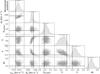 |
Fig. B.1 Corner plot showing posteriors for our injection test of model Loff. Vertical and horizontal black lines represent the true values at which our model was injected into the data. Despite the correlation among the parameters, our analysis is capable of retrieving the correct answer within 2σ for every parameter. |
Appendix C Comparison of intrinsic information content in HARPS-N and CARMENES
In this section, we investigate the distribution of strong neutral iron lines across the wavelength range probed by HARPS-N and CARMENES. We downloaded the VALD3 line list of neutral iron, and the partition function by Barklem & Collet (2016). We then computed the strength of each Fe I line at 4000 K — a temperature representative of the dayside atmosphere of KELT-9b— using standard formulas (e.g. Grimm & Heng 2015) and assuming local thermodynamic equilibrium. We argue that the line strength is a good proxy for the signal carried by each line, which is approximately true where no strong blending is seen, assuming that all lines probe similar pressures and that they are not saturated. The spectrum of KELT-9b should be dominated by atomic lines, and so we argue that the effect of blending should not be so strong as to be a hinderance. Pino et al. (2020) show the range of pressures probed by Fei lines observed with HARPS-N, which we expect to be similar to the range probed by CARMENES.
In addition, we take into account the planet-to-star flux ratio variation with wavelength, which is more favourable towards the red wavelengths probed by CARMENES. For this analysis, we weight the line strengths by the ratio of two blackbodies at temperatures of 4000 K to represent the planet, and 10000 K to represent the star.
Fig. C.1 shows a histogram of the line list weighted by the line strength at 4000 K, in arbitrary units. The blue histogram is additionally weighted by the planet-to-star flux ratio. While this additional factor increases the importance of the wavelength range probed by CARMENES compared to HARPS-N, blue wavelengths still seem to contain more information about Fe I for KELT-9b. However, this conclusion cannot be generalised to other planets (e.g. see Herman et al. 2022), as it depends on the location in pressure of the contribution functions of lines (hence, on the temperature-pressure profile and volume mixing ratio), and on blanketing and blending effects by other species which are likely weaker in KELT-9b.
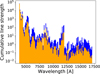 |
Fig. C.1 Cumulative line strength of neutral iron lines at 4000 K across the wavelength range probed by HARPS-N and CARMENES. The orange histogram only accounts for the line strengths, while the blue histogram additionally accounts for the planet-to-star flux ratio. |
Appendix D Corner plots for individual night retrievals with model 1C
In this section, we show corner plots displaying all the posteriors obtained for individual nights.
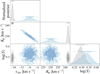 |
Fig. D.1 Posterior for the MCMC fit to HARPS-N Nl using model 1C (blue) compared to five nights combined (grey). |
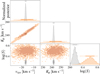 |
Fig. D.2 Posterior for the MCMC fit to HARPS-N N2 using model 1C (orange) compared to five nights combined (grey). |
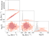 |
Fig. D.3 Posterior for the MCMC fit to CARMENES Nl using model 1C (red) compared to five nights combined (grey). |
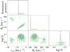 |
Fig. D.4 Posterior for the MCMC fit to CARMENES N2 using model 1C (green) compared to five nights combined (grey). |
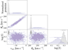 |
Fig. D.5 Posterior for the MCMC fit to HARPS-N N3 using model 1C (purple) compared to five nights combined (grey). |
Appendix E Corner plots for models 4C and 4E, and L, Loff and Lbase
In this section, we show corner plots displaying all the posteriors obtained for four scaling factor models and for the Lambert sphere model variations.
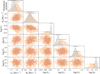 |
Fig. E.1 Corner plot showing posteriors for model 4C (orange). We overlay 1D posteriors for model 1C in grey. The posteriors for log S1 … log S4 are all compared to the posterior for the individual scaling factor log S of model 1C. We zoom into the 1σ and 2σ confidence interval regions for each parameter. |
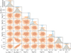 |
Fig. E.2 Corner plot showing posteriors for model 4E (orange). We overlay 1D posteriors for model 1E in blue. The posteriors for log S1 … log S4 are all compared to the posterior for the individual scaling factor log S of model 1E. We zoom into the 1σ and 2σ confidence interval regions for each parameter. |
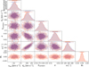 |
Fig. E.3 Corner plot showing posteriors for model Loff (red). We overlay posteriors for model L in purple. We zoom into the 1σ and 2σ confidence interval regions for each parameter. |
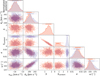 |
Fig. E.4 Corner plot showing posteriors for model Lbase (red). We overlay posteriors for model L in purple. We zoom into the 1σ and 2σ confidence interval regions for each parameter. The limit of our prior (SLambert > 0) is visible for the Lbase model. We discuss the clear correlation between S and SLambert in section 3.3. |
Appendix F Best-fit model parameter values and errors
In Table F.1 we report the full results of our retrievals on the five HARPS-N and CARMENES combined nights analysed. Each entry represents the 50th percentile of the Monte Carlo samples for each parameter, while 1σ intervals define the highest density region of the parameter range such that 95% of the sample is found in that region.
References
- Addison, B. C., Knudstrup, E., Wong, I., et al. 2021, AJ, 162, 292 [NASA ADS] [CrossRef] [Google Scholar]
- Allart, R., Pino, L., Lovis, C., et al. 2020, A&A, 644, A155 [NASA ADS] [CrossRef] [EDP Sciences] [Google Scholar]
- Astropy Collaboration (Robitaille, T.P., et al.) 2013, A&A, 558, A33 [NASA ADS] [CrossRef] [EDP Sciences] [Google Scholar]
- Astropy Collaboration (Price-Whelan, A.M., et al.) 2018, AJ, 156, 123 [NASA ADS] [CrossRef] [Google Scholar]
- Astropy Collaboration (Price-Whelan, A.M., et al.) 2022, ApJ, 935, 167 [NASA ADS] [CrossRef] [Google Scholar]
- Bard, A., & Kock, M. 1994, A&A, 282, 1014 [NASA ADS] [Google Scholar]
- Bard, A., Kock, A., & Kock, M. 1991, A&A, 248, 315 [NASA ADS] [Google Scholar]
- Barklem, P. S., & Collet, R. 2016, A&A, 588, A96 [NASA ADS] [CrossRef] [EDP Sciences] [Google Scholar]
- Barklem, P. S., Piskunov, N., & O’Mara, B.J. 2000, A&AS, 142, 467 [NASA ADS] [CrossRef] [EDP Sciences] [Google Scholar]
- Baxter, C., Désert, J.-M., Parmentier, V., et al. 2020, A&A, 639, A36 [EDP Sciences] [Google Scholar]
- Bell, T. J., & Cowan, N. B. 2018, ApJ, 857, L20 [Google Scholar]
- Bello-Arufe, A., Buchhave, L. A., Mendonça, J. M., et al. 2022, A&A, 662, A51 [NASA ADS] [CrossRef] [EDP Sciences] [Google Scholar]
- Beltz, H., Rauscher, E., Brogi, M., & Kempton, E. M. R. 2021, AJ, 161, 1 [Google Scholar]
- Beltz, H., Rauscher, E., Kempton, E. M. R., et al. 2022a, AJ, 164, 140 [NASA ADS] [CrossRef] [Google Scholar]
- Beltz, H., Rauscher, E., Roman, M. T., & Guilliat, A. 2022b, AJ, 163, 35 [NASA ADS] [CrossRef] [Google Scholar]
- Bonomo, A. S., Desidera, S., Benatti, S., et al. 2017, A&A, 602, A107 [NASA ADS] [CrossRef] [EDP Sciences] [Google Scholar]
- Borsa, F., Rainer, M., Bonomo, A. S., et al. 2019, A&A, 631, A34 [NASA ADS] [CrossRef] [EDP Sciences] [Google Scholar]
- Borsa, F., Giacobbe, P., Bonomo, A. S., et al. 2022, A&A, 663, A141 [NASA ADS] [CrossRef] [EDP Sciences] [Google Scholar]
- Brogi, M., & Line, M. R. 2019, AJ, 157, 114 [Google Scholar]
- Brogi, M., Snellen, I. A. G., de Kok, R. J., et al. 2013, ApJ, 767, 27 [NASA ADS] [CrossRef] [Google Scholar]
- Charbonneau, D., Allen, L. E., Megeath, S. T., et al. 2005, ApJ, 626, 523 [Google Scholar]
- Claudi, R., Benatti, S., Carleo, I., et al. 2017, Euro. Phys. J. Plus, 132, 364 [NASA ADS] [CrossRef] [Google Scholar]
- Collier Cameron, A., Horne, K., Penny, A., & James, D. 1999, Nature, 402, 751 [NASA ADS] [CrossRef] [Google Scholar]
- Collier Cameron, A., Horne, K., Penny, A., & Leigh, C. 2002, MNRAS, 330, 187 [NASA ADS] [CrossRef] [Google Scholar]
- Cont, D., Yan, F., Reiners, A., et al. 2021, A&A, 651, A33 [NASA ADS] [CrossRef] [EDP Sciences] [Google Scholar]
- Cosentino, R., Lovis, C., Pepe, F., et al. 2012, SPIE Conf. Ser., 8446, 84461V [Google Scholar]
- Deeg, H. J., & Belmonte, J. A. 2018, Handbook of Exoplanets (Berlin: Springer) [CrossRef] [Google Scholar]
- Dobbs-Dixon, I., & Blecic, J. 2022, ApJ, 929, 46 [NASA ADS] [CrossRef] [Google Scholar]
- Eastman, J., Siverd, R., & Gaudi, B. S. 2010, PASP, 122, 935 [Google Scholar]
- Eastman, J., Gaudi, B. S., & Agol, E. 2013, PASP, 125, 83 [Google Scholar]
- Ehrenreich, D., Lovis, C., Allart, R., et al. 2020, Nature, 580, 597 [Google Scholar]
- Feng, Y. K., Line, M. R., Fortney, J. J., et al. 2016, ApJ, 829, 52 [NASA ADS] [CrossRef] [Google Scholar]
- Fortney, J. J., Dawson, R. I., & Komacek, T. D. 2021, J. Geophys. Res. Planets, 126, e06629 [NASA ADS] [CrossRef] [Google Scholar]
- Fossati, L., Shulyak, D., Sreejith, A. G., et al. 2020, A&A, 643, A131 [NASA ADS] [CrossRef] [EDP Sciences] [Google Scholar]
- Fossati, L., Young, M. E., Shulyak, D., et al. 2021, A&A, 653, A52 [NASA ADS] [CrossRef] [EDP Sciences] [Google Scholar]
- Fuhr, J. R., Martin, G. A., & Wiese, W. L. 1988, J. Phys. Chem. Ref. Data, 17, 4 [Google Scholar]
- Gaudi, B. S., Stassun, K. G., Collins, K. A., et al. 2017, Nature, 546, 514 [NASA ADS] [Google Scholar]
- Giacobbe, P., Brogi, M., Gandhi, S., et al. 2021, Nature, 592, 205 [NASA ADS] [CrossRef] [Google Scholar]
- Gibson, N. P., Merritt, S., Nugroho, S. K., et al. 2020, MNRAS, 220 [Google Scholar]
- Gibson, N. P., Nugroho, S. K., Lothringer, J., Maguire, C., & Sing, D. K. 2022, MNRAS, 512, 4618 [NASA ADS] [CrossRef] [Google Scholar]
- Grimm, S. L., & Heng, K. 2015, ApJ, 808, 182 [NASA ADS] [CrossRef] [Google Scholar]
- Guilluy, G., Andretta, V., Borsa, F., et al. 2020, A&A, 639, A49 [EDP Sciences] [Google Scholar]
- Guilluy, G., Giacobbe, P., Carleo, I., et al. 2022, A&A, 665, A104 [NASA ADS] [CrossRef] [EDP Sciences] [Google Scholar]
- Helling, C., Gourbin, P., Woitke, P., & Parmentier, V. 2019, A&A, 626, A133 [NASA ADS] [CrossRef] [EDP Sciences] [Google Scholar]
- Herman, M. K., de Mooij, E. J. W., Nugroho, S. K., Gibson, N. P., & Jayawardhana, R. 2022, AJ, 163, 248 [NASA ADS] [CrossRef] [Google Scholar]
- Hoeijmakers, H. J., Ehrenreich, D., Heng, K., et al. 2018, Nature, 560, 453 [CrossRef] [Google Scholar]
- Hoeijmakers, H. J., Ehrenreich, D., Kitzmann, D., et al. 2019, A&A, 627, A165 [NASA ADS] [CrossRef] [EDP Sciences] [Google Scholar]
- Huang, C., Arras, P., Christie, D., & Li, Z.-Y. 2017, ApJ, 851, 150 [NASA ADS] [CrossRef] [Google Scholar]
- Hyndman, R. J. 1996, Am. Stat., 50, 120 [Google Scholar]
- Ivshina, E. S., & Winn, J. N. 2022, ApJS, 259, 62 [CrossRef] [Google Scholar]
- John, T. L. 1988, A&A, 193, 189 [NASA ADS] [Google Scholar]
- Johnson, M. C., Wang, J., Pai Asnodkar, A., et al. 2022, AAS J., submitted [arXiv:2205.12162] [Google Scholar]
- Jones, K., Morris, B. M., Demory, B. O., et al. 2022, A&A, 666, A118 [NASA ADS] [CrossRef] [EDP Sciences] [Google Scholar]
- Kasper, D., Bean, J. L., Line, M. R., et al. 2021, ApJ, 921, L18 [CrossRef] [Google Scholar]
- Kawahara, H. 2012, ApJ, 760, L13 [NASA ADS] [CrossRef] [Google Scholar]
- Kitzmann, D., Heng, K., Rimmer, P. B., et al. 2018, ApJ, 863, 183 [Google Scholar]
- Komacek, T. D., Showman, A. P., & Tan, X. 2017, ApJ, 835, 198 [NASA ADS] [CrossRef] [Google Scholar]
- Kreidberg, L., Line, M. R., Parmentier, V., et al. 2018, AJ, 156, 17 [NASA ADS] [CrossRef] [Google Scholar]
- Kupka, F., Piskunov, N., Ryabchikova, T.A., Stempels, H.C., & Weiss, W.W. 1999, A&AS, 138, 119 [NASA ADS] [CrossRef] [EDP Sciences] [Google Scholar]
- Kupka, F. G., Ryabchikova, T. A., Piskunov, N. E., Stempels, H. C., & Weiss, W. W. 2000, Balt. Astron., 9, 590 [Google Scholar]
- Kurucz, R. L. 2014, Robert L. Kurucz on-line Database of Observed and Predicted Atomic Transitions (Cambridge: Harvard-Smithsonian Center for Astrophysics) [Google Scholar]
- Line, M. R., Brogi, M., Bean, J. L., et al. 2021, Nature, 598, 580 [NASA ADS] [CrossRef] [Google Scholar]
- Lothringer, J. D., Barman, T., & Koskinen, T. 2018, ApJ, 866, 27 [NASA ADS] [CrossRef] [Google Scholar]
- Lothringer, J. D., Rustamkulov, Z., Sing, D. K., et al. 2021, ApJ, 914, 12 [CrossRef] [Google Scholar]
- Mansfield, M., Bean, J. L., Stevenson, K. B., et al. 2020, ApJ, 888, L15 [Google Scholar]
- Mansfield, M., Line, M. R., Bean, J. L., et al. 2021, Nat. Astron., 5, 1224 [CrossRef] [Google Scholar]
- Mikal-Evans, T., Sing, D. K., Barstow, J. K., et al. 2022, Nat. Astron., 6, 471 [NASA ADS] [CrossRef] [Google Scholar]
- Nugroho, S. K., Gibson, N. P., de Mooij, E. J. W., et al. 2020, ApJ, 898, L31 [Google Scholar]
- Nymeyer, S., Harrington, J., Hardy, R. A., et al. 2011, ApJ, 742, 35 [NASA ADS] [CrossRef] [Google Scholar]
- O’Brian, T.R., Wickliffe, M.E., Lawler, J.E., Whaling, W., & Brault, J.W. 1991, J. Opt. Soc. Am. B Opt. Phys., 8, 1185 [CrossRef] [Google Scholar]
- Pai Asnodkar, A., Wang, J., Eastman, J. D., et al. 2022, AJ, 163, 155 [NASA ADS] [CrossRef] [Google Scholar]
- Parmentier, V., & Crossfield, I. J. M. 2018, in Handbook of Exoplanets, eds. H.J. Deeg, & J.A. Belmonte (Berlin: Springer), 116 [Google Scholar]
- Parmentier, V., Line, M. R., Bean, J. L., et al. 2018, A&A, 617, A110 [NASA ADS] [CrossRef] [EDP Sciences] [Google Scholar]
- Pelletier, S., Benneke, B., Darveau-Bernier, A., et al. 2021, AJ, 162, 73 [NASA ADS] [CrossRef] [Google Scholar]
- Perna, R., Menou, K., & Rauscher, E. 2010, ApJ, 719, 1421 [NASA ADS] [CrossRef] [Google Scholar]
- Pino, L., Désert, J.-M., Brogi, M., et al. 2020, ApJ, 894, L27 [Google Scholar]
- Piskunov, N. E., Kupka, F., Ryabchikova, T.A., Weiss, W.W., & Jeffery, C.S. 1995, A&AS, 112, 525 [NASA ADS] [Google Scholar]
- Poretti, E., Boccato, C., Claudi, R., et al. 2016, Mem. Soc. Astron. Italiana, 87, 141 [NASA ADS] [Google Scholar]
- Quirrenbach, A., Amado, P. J., Caballero, J. A., et al. 2016, SPIE Conf. Ser., 9908, 990812 [Google Scholar]
- Quirrenbach, A., Amado, P. J., Ribas, I., et al. 2018, SPIE Conf. Ser., 10702, 107020W [Google Scholar]
- Ragozzine, D., & Wolf, A. S. 2009, ApJ, 698, 1778 [Google Scholar]
- Rainer, M., Borsa, F., Pino, L., et al. 2021, A&A, 649, A29 [NASA ADS] [CrossRef] [EDP Sciences] [Google Scholar]
- Rauscher, E., & Menou, K. 2012, ApJ, 750, 96 [NASA ADS] [CrossRef] [Google Scholar]
- Ryabchikova, T. A., Piskunov, N. E., Kupka, F., & Weiss, W. W. 1997, Balt. Astron., 6, 244 [NASA ADS] [Google Scholar]
- Ryabchikova, T., Piskunov, N., Kurucz, R. L., et al. 2015, Phys. Scr, 90, 054005 [Google Scholar]
- Savel, A. B., Kempton, E. M. R., Malik, M., et al. 2022, ApJ, 926, 85 [NASA ADS] [CrossRef] [Google Scholar]
- Scandariato, G., Borsa, F., Sicilia, D., et al. 2021, A&A, 646, A159 [NASA ADS] [CrossRef] [EDP Sciences] [Google Scholar]
- Seidel, J. V., Ehrenreich, D., Pino, L., et al. 2020, A&A, 633, A86 [NASA ADS] [CrossRef] [EDP Sciences] [Google Scholar]
- Showman, A. P., & Polvani, L. M. 2011, ApJ, 738, 71 [Google Scholar]
- Shporer, A., O’Rourke, J.G., Knutson, H.A., et al. 2014, ApJ, 788, 92 [NASA ADS] [CrossRef] [Google Scholar]
- Snellen, I. A. G., Brandl, B. R., de Kok, R. J., et al. 2014, Nature, 509, 63 [Google Scholar]
- Southworth, J. 2008, MNRAS, 386, 1644 [NASA ADS] [CrossRef] [Google Scholar]
- Stephan, A. P., Wang, J., Cauley, P. W., et al. 2022, ApJ, 931, 111 [NASA ADS] [CrossRef] [Google Scholar]
- Stevenson, K. B. 2016, ApJ, 817, L16 [NASA ADS] [CrossRef] [Google Scholar]
- Stevenson, K. B., Désert, J.-M., Line, M. R., et al. 2014, Science, 346, 838 [Google Scholar]
- Stock, J. W., Kitzmann, D., Patzer, A. B. C., & Sedlmayr, E. 2018, MNRAS, 479, 865 [NASA ADS] [Google Scholar]
- Tan, X., & Komacek, T. D. 2019, ApJ, 886, 26 [Google Scholar]
- Toon, O. B., McKay, C. P., Ackerman, T. P., & Santhanam, K. 1989, J. Geophys. Res., 94, 16287 [Google Scholar]
- van Sluijs, L., Birkby, J. L., Lothringer, J., et al. 2022, MNRAS, submitted [arXiv:2203.13234] [Google Scholar]
- von Essen, C., Mallonn, M., Borre, C. C., et al. 2020, A&A, 639, A34 [NASA ADS] [CrossRef] [EDP Sciences] [Google Scholar]
- Wardenier, J. P., Parmentier, V., Lee, E. K. H., Line, M. R., & Gharib-Nezhad, E. 2021, MNRAS, 506, 1258 [NASA ADS] [CrossRef] [Google Scholar]
- Wardenier, J. P., Parmentier, V., & Lee, E. K. H. 2022, MNRAS, 510, 620 [Google Scholar]
- Wong, I., Shporer, A., Kitzmann, D., et al. 2020, AJ, 160, 88 [Google Scholar]
- Yan, F., Pallé, E., Reiners, A., et al. 2020, A&A, 640, L5 [NASA ADS] [CrossRef] [EDP Sciences] [Google Scholar]
- Zhang, J., Kempton, E. M. R., & Rauscher, E. 2017, ApJ, 851, 84 [Google Scholar]
- Zhang, M., Knutson, H. A., Kataria, T., et al. 2018, AJ, 155, 83 [Google Scholar]
- Zhang, Y., Snellen, I. A. G., Wyttenbach, A., et al. 2022, A&A, 666, A47 [NASA ADS] [CrossRef] [EDP Sciences] [Google Scholar]
Observed in GIARPS (GIANO-B + HARPS-N) mode (Claudi et al. 2017); but we only use the HARPS-N data in this work.
Additional references specific to the used Fe I line list: Kurucz (2014), Bard et al. (1991), Bard & Kock (1994), Barklem et al. (2000), O’Brian et al. (1991), Fuhr et al. (1988).
We verified that optimising this additional scaling factor between 10 and 0.001% of the model flux has no impact on the result.
AIC and BIC should be computed in the maximum likelihood, which we have approximated with the median of the posterior. With a flat prior and perfectly symmetrical posteriors, this is a correct assumption.
All Tables
All Figures
|
Fig. 1 Schematic representation of the orbit of KELT-9 b to scale, with the orbital phases covered in this study colour-coded according to observing night (Blue: HARPS-N N1; Orange: HARPS-N N2; Purple: HARPS-N N3; Red: CARMENES N1; Green: CARMENES N2). The exoplanet orbits counterclockwise (curved arrow), and the observer is positioned at the bottom of the figure. |
| In the text | |
|
Fig. 2 Effects of telluric removal on the signal from KELT-9 b. Left: best-fit Fe I emission model Doppler-shifted based on the orbital parameters of KELT-9 b (panel a), injected on top of the first night of HARPS-N data, and passed through the analysis described in Sect. 2.2.2. The signal is recovered with evident alterations, as shown in the reference frame of the observer (panel b) and in the planet’s rest frame (panel c). Top-right: recovered amplitude of a strong injected Fe line as a function of orbital phase (solid) versus its amplitude at injection (dashed). Bottom-right: percent loss of the Fe signal due to the telluric-removal analysis. Nearly 100% of the signal is lost around quadrature. |
| In the text | |
|
Fig. 3 Posterior distributions of parameters of model 1C fit with an MCMC to HARPS-N N1 (blue), HARPS-N N2 (orange), CARMENES N1 (red), CARMENES N2 (green), HARPS-N N3 (purple), and all five nights combined (black). Lower panels: normalised posteriors (higher peak for better constrained parameters), and the marked improvement obtained when combining all data sets. Upper panels: 1σ (dark colour) and 2σ (light colour) confidence intervals obtained from the corresponding posteriors in the lower panels. |
| In the text | |
|
Fig. 4 Posterior for the MCMC fit of models 1C (circular orbit, black histograms) and 1E (eccentric orbit, blue histograms). The 1σ and 2σ confidence intervals are indicated with darker and lighter shades, respectively. |
| In the text | |
|
Fig. 5 Time-resolved confidence intervals as a function of the planet rest-frame velocity obtained by binning (i.e. co-adding) the individual likelihood functions by 0.02 in orbital phase. Black represents 1σ deviations from the best-fit rest-frame velocity in each phase bin, and grey represents 2σ deviations. The left and centre panels show results for the 1C (circular) and 1E (eccentric) models, respectively, when fixing all the model parameters at their best-fit value, i.e. the median of the posterior distribution. Horizontal black dashed lines indicate phases corresponding to ingress and egress, and a vertical red dashed line indicates the best-fit planet rest-frame. The right panel represents the total S/N achieved within each phase bin, with HARPS-N (lighter pink) and CARMENES (darker purple). |
| In the text | |
|
Fig. 6 Posterior distribution for the scaling factors of models 1C and 4C (left panel), and IE and 4E (middle panel). Right panel: colour-coded phase ranges corresponding to each of the five parameters for each panel. |
| In the text | |
|
Fig. 7 Results of our search for variations in the intensity of the observed neutral iron lines. Upper panel: 100 draws from the posterior for scaling factors as a function of phase obtained by fitting models IE (orange), 4E (blue), L (black), Loff (red) and Lbase (green) to the data. The phase coverage of the data is shown in the lower panel, in terms of the S/N of stellar spectra in each phase bin (HARPS-N: lighter pink; CARMENES: darker purple). Where multiple nights cover the same orbital phase bin, their contributions are summed in quadrature. |
| In the text | |
|
Fig. 8 Comparison of planet trail with predictions of radial velocity anomaly induced by rotation and different wind patterns. Lower panel: planetary trail obtained in the best-fit circular orbit reference frame (same as left panel of Fig. 5, but zooming onto smaller radial velocity displacements from the best-fit circular orbit rest frame), and comparison with predictions of net Doppler shift in different cases: pure rotation (blue dashed curve), east-west wind of 10 km s−1 (green dashed curve), and day-to-night wind of 5 km s−1 (orange dot-dashed curve). Upper panel: contribution to Doppler shift from the portion of the planet disk seen at different phases due to the two wind geometries considered and planet rotation. Black portions of the disk correspond to the night-side, while red(blue) portions correspond to regions producing red(blue)shifted lines. Less weight should be given to phase bins close to quadrature (φ < 0.35; φ > 0.65) because of the detrimental effect of our analysis on the S/N in this phase range (see Fig. 2). |
| In the text | |
|
Fig. B.1 Corner plot showing posteriors for our injection test of model Loff. Vertical and horizontal black lines represent the true values at which our model was injected into the data. Despite the correlation among the parameters, our analysis is capable of retrieving the correct answer within 2σ for every parameter. |
| In the text | |
|
Fig. C.1 Cumulative line strength of neutral iron lines at 4000 K across the wavelength range probed by HARPS-N and CARMENES. The orange histogram only accounts for the line strengths, while the blue histogram additionally accounts for the planet-to-star flux ratio. |
| In the text | |
|
Fig. D.1 Posterior for the MCMC fit to HARPS-N Nl using model 1C (blue) compared to five nights combined (grey). |
| In the text | |
|
Fig. D.2 Posterior for the MCMC fit to HARPS-N N2 using model 1C (orange) compared to five nights combined (grey). |
| In the text | |
|
Fig. D.3 Posterior for the MCMC fit to CARMENES Nl using model 1C (red) compared to five nights combined (grey). |
| In the text | |
|
Fig. D.4 Posterior for the MCMC fit to CARMENES N2 using model 1C (green) compared to five nights combined (grey). |
| In the text | |
|
Fig. D.5 Posterior for the MCMC fit to HARPS-N N3 using model 1C (purple) compared to five nights combined (grey). |
| In the text | |
|
Fig. E.1 Corner plot showing posteriors for model 4C (orange). We overlay 1D posteriors for model 1C in grey. The posteriors for log S1 … log S4 are all compared to the posterior for the individual scaling factor log S of model 1C. We zoom into the 1σ and 2σ confidence interval regions for each parameter. |
| In the text | |
|
Fig. E.2 Corner plot showing posteriors for model 4E (orange). We overlay 1D posteriors for model 1E in blue. The posteriors for log S1 … log S4 are all compared to the posterior for the individual scaling factor log S of model 1E. We zoom into the 1σ and 2σ confidence interval regions for each parameter. |
| In the text | |
|
Fig. E.3 Corner plot showing posteriors for model Loff (red). We overlay posteriors for model L in purple. We zoom into the 1σ and 2σ confidence interval regions for each parameter. |
| In the text | |
|
Fig. E.4 Corner plot showing posteriors for model Lbase (red). We overlay posteriors for model L in purple. We zoom into the 1σ and 2σ confidence interval regions for each parameter. The limit of our prior (SLambert > 0) is visible for the Lbase model. We discuss the clear correlation between S and SLambert in section 3.3. |
| In the text | |
Current usage metrics show cumulative count of Article Views (full-text article views including HTML views, PDF and ePub downloads, according to the available data) and Abstracts Views on Vision4Press platform.
Data correspond to usage on the plateform after 2015. The current usage metrics is available 48-96 hours after online publication and is updated daily on week days.
Initial download of the metrics may take a while.