| Issue |
A&A
Volume 668, December 2022
|
|
|---|---|---|
| Article Number | A95 | |
| Number of page(s) | 23 | |
| Section | Galactic structure, stellar clusters and populations | |
| DOI | https://doi.org/10.1051/0004-6361/202244453 | |
| Published online | 08 December 2022 | |
Mapping Milky Way disk perturbations in stellar number density and vertical velocity using Gaia DR3
1
Dark Cosmology Centre, Niels Bohr Institute, University of Copenhagen, Jagtvej 128, 2200 Copenhagen N, Denmark
e-mail: This email address is being protected from spambots. You need JavaScript enabled to view it.
2
Department of Physics, Engineering Physics, and Astronomy, Queen’s University, Kingston K7L 3X5, Canada
3
School of Physics & Astronomy, University of Nottingham, University Park, Nottingham NG7 2RD, UK
Received:
7
July
2022
Accepted:
27
October
2022
Abstract
We have mapped the number density and mean vertical velocity of the Milky Way’s stellar disk out to roughly two kiloparsecs from the Sun using Gaia Data Release 3 (DR3) and complementary photo-astrometric distance information from StarHorse. For the number counts, we carefully masked spatial regions that are compromised by open clusters, great distances, or dust extinction and used Gaussian processes to arrive at a smooth, non-parametric estimate for the underlying number density field. We find that the number density and velocity fields depart significantly from an axisymmetric and mirror-symmetric model. These departures, which include projections of the Gaia phase-space spiral, signal the presence of local disturbances in the disk. We identify two features that are present in both stellar number density and mean vertical velocity. One of these features appears to be associated with the Local Spiral Arm. It is most prominent at small heights and is largely symmetric across the mid-plane of the disk. The density and velocity field perturbations are phase-shifted by roughly a quarter wavelength, suggesting a breathing mode that is propagating in the direction of Galactic longitude l ∼ 270 deg. The second feature is a gradient in the stellar number density and mean vertical velocity with respect to galactocentric radius. This feature, which extends across the entire region of our analysis, may be associated with the extension of the Galactic warp into the solar neighbourhood in combination with more localised bending waves.
Key words: Galaxy: kinematics and dynamics / Galaxy: disk / solar neighborhood / astrometry
© The Authors 2022
 Open Access article, published by EDP Sciences, under the terms of the Creative Commons Attribution License (https://creativecommons.org/licenses/by/4.0), which permits unrestricted use, distribution, and reproduction in any medium, provided the original work is properly cited.
This article is published in open access under the Subscribe-to-Open model. This email address is being protected from spambots. You need JavaScript enabled to view it. to support open access publication.
1. Introduction
Gaia Data Release 3 (Gaia DR3) provides the measurements necessary to model the six-dimensional phase-space distribution function (DF) of stars within a few kiloparsecs of the Sun (Gaia Collaboration 2016, 2022a,b) and thereby test our understanding of stellar dynamics and galactic evolution. However, analysis of the full phase-space DF is challenging due to the curse of dimensionality and the difficulty of visualising structure in six dimensions. In this paper, we focus on the stellar number density n and mean vertical velocity  , which are derived from velocity moments of the DF. Our interest in these quantities stems from recent observations of dynamical features in the disk associated with the structure perpendicular to the Galactic mid-plane. These include the number count asymmetry about the mid-plane (Widrow et al. 2012; Yanny & Gardner 2013; Bennett & Bovy 2019; Everall et al. 2022a), bending and breathing motions Widrow et al. (2012), Williams et al. (2013), Carlin et al. (2013), Gaia Collaboration (2018, 2022a), and the phase-space spiral in the (Z, W)-plane (Antoja et al. 2018). There is also evidence that the disk is corrugated beyond the solar circle from observations of both n (Xu et al. 2015) and
  (Schönrich & Dehnen 2018; Friske & Schönrich 2019).
In his seminal work on the vertical structure of the Milky Way, Oort (1932) combined observations of n and  in the solar neighborhood to infer the vertical acceleration az as a function of Z. The essence of the calculation can be understood from dimensional considerations; near the mid-plane
  , where ΔW and ΔZ are characteristic widths of the disk in Z and W, and Ωz is the frequency of vertical oscillations. In principle, simultaneous measurements of the spatial and velocity distributions associated with a disturbance of the disk would similarly allow us to study its dynamics. For example, armed with measurements of the displacement of the mid-plane and mean vertical velocity, we might be able to test theories of bending modes in the disk (see Sellwood 2013 and references therein).
To date, most of the dynamical features mentioned above have been detected in either n or W. One notable exception is the phase spiral, which is seen in number counts in the (Z, W) phase-space. The phase spiral almost certainly arises from the incomplete phase mixing of a perturbation to the disk and the presence of information in both Z and W allows us to date the perturbation (e.g. Antoja et al. 2018; Laporte et al. 2019; Li & Widrow 2021; Widmark et al. 2022a). One of the main goals of this paper is to find other examples of perturbations that can be identified in both n and W and combine these two spatially varying fields in order to learn about the time-varying nature of disk perturbations.
The main challenge in inferring n comes from understanding the selection effects. In particular, the Gaia selection function is highly complex (Boubert & Everall 2020; Everall et al. 2022b; Everall & Boubert 2022; Rybizki et al. 2021; Cantat-Gaudin et al. 2022); it mainly depends on stellar crowding and the Gaia scanning law and brightness limits, with the additional confounding issues of dust reddening and extinction. These different factors have a spatial dependence, but are independent with respect to velocity. Modelling significant selection effects is often challenging, making it difficult to accurately extract the stellar number density distribution. By comparison, it is more straightforward to derive the mean velocity field as a function of spatial position (e.g. Gaia Collaboration 2018; Martinez-Medina et al. 2022) since the spatially dependent selection does not induce a strong systematic bias but only lowers the amount of available data. On the other hand, velocity measurements require parallax, proper motion, and radial velocity measurements. At present, the number of stars in Gaia where this is possible is a factor of ∼30 smaller than the total number of stars in the survey.
We modelled the spatial distribution of stars in the Galactic disk within a distance of roughly two kiloparsecs using data from Gaia DR3 Gaia Collaboration (2022b), supplemented with photo-astrometric distances from StarHorse (Anders et al. 2022). We assumed that the three-dimensional stellar number density distribution is a Gaussian process (GP) and used GP regression to estimate the underlying smooth number density field in a non-parametric way that does not rely on any symmetry assumptions such as axisymmetry or mirror symmetry about the Galactic plane. We carefully masked any spatial region that is compromised by a large distance, dust extinction, or the presence of open clusters. Thanks to the inherent property of smoothness of GPs, a masked spatial volume is still informed by its unmasked spatial neighbourhood. In this manner, we were able to construct a model-independent yet robust three-dimensional map of the stellar number density distribution within a distance of a few kiloparsecs. We also mapped the mean vertical velocity field  using a similar approach, for example masking open clusters, although we simply calculated the mean value in fixed spatial volumes without any GP regression. For a GP model of the velocity field, see Nelson & Widrow (2022).
This article is structured as follows. In Sect. 2 we present the data and define our coordinate system. We describe our method for mapping the stellar number density distribution in Sect. 3 and our method for mapping the vertical velocity distribution in Sect. 4. In Sect. 5 we present our results. In the final Sects. 6 and 7, we discuss and conclude.
2. Data
We used data from Gaia DR3, supplemented with photo-astrometric distance and dust extinction information from StarHorse (Anders et al. 2022), which is available for Gaia stars with an apparent magnitude mG < 18.5. We analysed four different stellar populations defined by a range in absolute magnitude in the GaiaG-band according to MG ∈ (0, 1], (1, 2], (2, 3, and (3, 4]. A colour-magnitude diagram illustrating our data sample cuts can be found in Fig. 1. In this paper, all colours and absolute magnitudes (but not apparent magnitudes) are taken directly from the StarHorse catalogue, and thus include a correction for dust reddening or extinction. We plot the age distribution of the respective stellar samples in Appendix A.
 |
Fig. 1. Colour-magnitude diagram of stars in StarHorse within a distance of 400 pc. The panel on the right side shows the 1D absolute magnitude histogram. The dashed lines correspond to the magnitude cuts of our four data samples. The colour and absolute magnitude values are intrinsic and dust-corrected as given directly by the StarHorse catalogue. |
We used the Cartesian heliocentric coordinates X = (X, Y, Z), which point in the directions of the Galactic centre, Galactic rotation, and Galactic north. In terms of the Galactic longitude and latitude, written l and b, these coordinates are defined according to
 (1)
(1)
where d is the distance from the solar position. We also made use of the galactocentric cylindrical radius, given by
 (2)
(2)
where we assumed a value of R⊙ = 8.2 kpc for the Sun’s distance from the Galactic centre (consistent with, e.g. McMillan 2016).
The time-derivatives of these spatial positions, dX/dt, give the velocities in the solar rest-frame. In this work, we focused on the vertical velocity, which is given by
 (3)
(3)
where kμ = 4.74057 yr mas−1 kpc−1 km s−1 is a unit conversion constant, μb is the latitudinal proper motion, and vRV is the radial velocity.
We accounted for the statistical uncertainties in number counts while neglecting observational uncertainties in the positions of individual stars. For the spatial positions of stars, we used the Gaia DR3 values for Galactic latitude and longitude and the StarHorse median value for the distance (labelled dist50 in that catalogue). When calculating the velocities, we used a similar procedure, neglecting observational uncertainties for the proper motions and radial velocity, although with the data quality cuts described in Sect. 4.
The relative precision of StarHorse distances is 3% at the bright end of the luminosity function but only 15% for mG ∼ 17 (see Fig. 13 in Anders et al. 2022). The spatial volume we studied is potentially problematic due to the high rate of dust extinction and stellar crowding. At a distance of a few kiloparsecs, even a relative uncertainty of a few percent is significant for our purposes, especially where there are strong degeneracies between distance and dust extinction. The data cuts we applied in order to circumvent these issues are described below in Sect. 3.1.
3. Stellar number density distribution
For each of our four stellar populations, defined by different cuts in absolute magnitude, we carefully masked spatial volumes that were compromised by large distances, high dust extinction, or the presence of open clusters. In the remaining spatial volume, where we could consider the data sample to be complete, we fitted a three-dimensional stellar number density distribution function using a GP. These steps are described in detail below.
3.1. Masks
Our strategy was to choose a spatial volume and range in apparent magnitude that minimised completeness issues. Specifically, we limited ourselves to mG in the range of 6–18, where the Gaia completeness function is close to unity, typically with deviations that are a few percent at most (Everall & Boubert 2022; Cantat-Gaudin et al. 2022). Furthermore, we masked areas of the sky where the number density is biased by the presence of open clusters. For this purpose, we constructed a mask function, written mask(X), which can either take a value of either zero or unity at every point in three-dimensional space. Any unmasked spatial volume was assumed to be complete.
We began by constructing a three-dimensional dust extinction map as a function of the angles l and b and the cylindrical radius  . We divided the (l, b) sky using a HEALPix map of order 7 (corresponding to an angular resolution of 0.46 degrees) and divided Rcyl into segments of width 100 pc. Each combination of the Rcyl segment and (l, b)-pixel corresponded to its own spatial volume for which we calculated the 80th percentile of dust extinction using StarHorse data (column ag50) for all stars with MG < 6 mag. Although we binned in terms of Rcyl, the map can equally well be understood in terms of heliocentric distance with a resolution in distance that depends on b.
Within each of these three-dimensional (l, b, Rcyl) volumes, the mask function was set to unity only where it was fulfilled that
 (4)
(4)
This criterion ensured that the non-masked data of some given spatial position have a distribution of apparent magnitudes that falls largely below 17, with only a weaker tail of stars that were dimmer than this limit. In this sense, using the 80th dust extinction percentile is a conservative measure.
We also masked the spatial volume where open clusters affected the stellar number density or obscured the field of view. We used the catalogue of open clusters from Cantat-Gaudin et al. (2018). For each open cluster, we assumed an angular size given by two times its half-light radius (r50 in the open cluster catalogue). Using the same sky map as defined for the dust mask above, we masked any spatial volume where the (l, b)-pixel overlapped with an open cluster’s angular area and the spatial distance extended beyond the fifth percentile distance of the open cluster (d05 in the open cluster catalogue). In doing so, we masked the spatial volumes that lie behind the sight-line of an open cluster, thereby mitigating incompleteness effects that may arise from stellar crowding.
The mask functions of our stellar samples can be seen in Fig. 2. The circular patches are masked due to open clusters, while the remaining more complex structure arises from dust extinction and the limit in apparent magnitude as defined in Eq. (4). The four data samples shown in the figure differ in their spatial extent, where the brightest sample reaches greater distances.
 |
Fig. 2. Upper distance limit, given by Eq. (4), as a function of angles l and b, for our four data samples. The centre of the map is in the direction of the Galactic centre, while positive b is pointing upwards and positive l is pointing to the right. |
In addition to these upper distance constraints, we also masked the nearby spatial volume in order to avoid stars that are too bright. We set a lower limit in distance, requiring that this criterion was fulfilled:
 (5)
(5)
where MG, low is the lower absolute magnitude bound of the data sample. This distance limit, in combination with the cuts in absolute magnitude, ensures that a star in our sample could never be brighter than mG = 6, regardless of dust extinction.
3.2. Number count and number density
The data for our GP analysis were reduced in the following way. We divided the spatial volume into a three-dimensional Cartesian grid with a 100 pc spacing in X and Y, and a 10 pc spacing in Z. We chose a smaller grid spacing in the Z direction, since the scale length for variations normal to the Galactic plane is smaller than the scale length for variations parallel to the Galactic plane. Furthermore, because we wished to study the Galactic disk, we restricted ourselves to |Z|≤800 pc. Each volume cell, written Vi, j, k, was labelled by the triplet of indices (i, j, k), which sets its spatial boundaries according to
 (6)
(6)
These volume cells could be partly or completely masked by the mask function described above.
The stellar number count in a given volume cell was related to its number density in the following way. Each volume cell had its specific number count, written Ni, j, k, given by the number of stars that remained in the volume cell after applying the mask function. We also associated each volume cell with an effective volume, written Ωi, j, k, corresponding to the non-masked volume within that cell:
 (7)
(7)
The effective volume of each cell was calculated numerically via Monte Carlo integration, and took values in the range [0, 105] pc3. These quantities were unique for each separate data sample.
For each volume cell that was not completely masked, the stellar number density was given by
 (8)
(8)
We took the associated statistical uncertainty of ni, j, k to be
 (9)
(9)
which corresponds to a Poisson count uncertainty in the limit of high data counts. We added a number 5 in quadrature in the nominator in order to decrease the statistical power where the data count is very low. Because we estimated the uncertainty from the data count, rather than from an underlying model that generates it, this statistical uncertainty was often underestimated especially for data bins with low number counts. We were mainly interested in the results where the number count was fairly high and the added number 5 was negligible; however, adding this number was necessary in order to avoid fitting artefacts, due to very low number count values at large distances from the Galactic mid-plane or where Ωi, j, k was close to zero. Choosing a slightly different number did not significantly alter our results.
The disk plane projections of number counts, after masks had been applied, can be seen in Fig. 3. The total number of volume cells that were not completely masked (i.e. Ωi, j, k > 0 pc3) was equal to 1 005 181, 806 270, 584 684, 310 122 for our four data samples (from brightest to dimmest). The total number of stars in the non-masked spatial volume are 4 613 344, 3 307 223, 6 820 434, 13 854 829.
 |
Fig. 3. Stellar number counts per area cell in the (X, Y)-plane, for our four data samples (specified in the top right corners), after masks have been applied. The arrows in the rightmost panel show the direction of the Galactic centre and the direction of Galactic rotation. The axis ranges are shared between all panels. |
3.3. Gaussian process fit
In this section, we describe how we modelled the normalised number counts as a GP. GP methods allow us to infer or interpolate an underlying function given a finite number of function observations. The main attraction of GPs for this work is that they allowed us to model the stellar number density n(X) as a smooth and differentiable function without imposing a parametric form that presupposes constraints such as Galactic axisymmetry. In addition, data uncertainties can be incorporated into GP modelling as long as they are approximately Gaussian.
Formally, a GP is a collection of random variables with the property that any finite subset of these variables has a multivariate normal distribution (see, e.g. Rasmussen & Williams 2005). The probability distribution function (PDF) for 𝒩 random variables from a GP is therefore defined by an 𝒩 × 𝒩 covariance matrix. In our case, the variables were the normalised number counts as labelled by i, j, k, while the elements of the covariance matrix depended on the distances between pairs of volume bins through a function usually called the kernel. In this paper, we used the radial basis function kernel, guaranteeing continuity and smoothness, for which the covariance matrix element for two bins with grid indices (i, j, k) and (i′,j′,k′) is
 (10)
(10)
The parameters A, lx, ly, and lz determine the overall variance and length scales associated with structure in the number counts. Proper choice of these hyperparameters is essential to finding a suitable model.
If we wished to infer the number counts at some new position X*, the joint PDF for 𝒩 data points and the new point is defined by an (𝒩 + 1)-dimensional Gaussian. On the other hand, the conditional PDF for the new point given the data is found by marginalising over the data via the Bayes theorem. Since the PDFs are all Gaussian, the marginalisation integrals can be done analytically. However, for this step, we must invert the N × N data covariance matrix, which is an 𝒪(N3) operation that requires 𝒪(N2) of rapid-access memory.
An exact GP analysis of our full data set was unfeasible given the large number of measurements and the CPU and RAM requirements of the GP calculation. There are numerous approximation schemes such as the inducing point method that allow us to apply GP regression to very large data sets (see Titsias 2009 and references therein). Here, we took the simple approach of applying GP regression to smaller spatial sub-volumes, rather than to the complete spatial volume all at once. For each area cell in the (X, Y)-plane, we fitted a new GP to its surroundings, including all other area cells within 650 pc (i.e.  ). The GP was fitted to the normalised number count
  , with its associated uncertainty
  .
.
In terms of the hyperparameters of the GP, as expressed in Eq. (10), we set the variance A to be equal to the variance of the normalised number count in the non-masked volume cells and used the spatial correlation scale lengths (lx, ly, lz) = (300, 300, 100) pc. Due to the computational cost and the shortcut of implementing GPs in sub-volumes, we did not attempt to fit the hyperparameters. Even if fitting the hyperparameters were computationally feasible, it still might not be desirable. The hyperparameters were specifically chosen such that the stellar number density fits would have certain properties of being correlated over reasonable spatial scales. Choosing a smaller correlation scale lengths could make it too sensitive to perturbations and systematic issues on smaller spatial scales. For example, there are degeneracies between parallax and absolute magnitude, as well as with the three-dimensional distribution of dust, giving rise to spatially correlated systematic errors, potentially on smaller scales. Our choice is further discussed and motivated in the beginning of Sect. 5.
3.4. Symmetric analytic function
For our non-parametric GP fit to the data, we were mainly interested in the perturbations with respect to some smooth background, and in which ways the symmetries of the Galactic disk are broken. In order to study these residuals, we also performed a parametric fit to our data using an analytic stellar number density distribution function, which was fully axisymmetric and mirror symmetric across the mid-plane. For this purpose, we used a mixture model of three disk components that take a functional form
 (11)
(11)
It has ten free parameters: ai is the respective amplitude of the three disk components, Li is their scale lengths, Hi is their scale heights, and Z⊙ is the height of the Sun with respect to the disk mid-place. We constrained ai to be positive, Li > 500 pc, and Hi > 100 pc.
We fitted fsymm. to the measured stellar densities in the non-masked spatial volume by maximising a Gaussian likelihood with the Adam optimiser (Kingma & Ba 2014). We used the same normalised stellar number count and statistical uncertainty as are defined in Eqs. (8) and (9), to the spatial volume that includes all area cells where the mean effective fractional volume for |Z|< 500 pc was larger than 50%. For each of our four data samples, we performed separate fits of fsymm.. The fitted parameters are found in Appendix B, where we also discuss some additional tests (e.g. fitting a smaller or larger number of disk components).
The main purpose of this function is to facilitate the visualisation of the GP model and serve as a smooth and symmetric background distribution for comparison purposes. For this reason, we refrain from making any strong physical interpretation of this function in isolation.
4. Vertical velocity distribution
In addition to the stellar number density field, we also studied the vertical component of the velocity field. We calculated the mean vertical velocity of our four stellar samples as a function of spatial position. We did so from the radial velocity sample, requiring a radial velocity uncertainty lower than 5 km s−1. The vertical velocity of each such star was given directly by its StarHorse distance (dist50) and Gaia DR3 velocity information (neglecting observational uncertainties). We also produced results with stronger data quality cuts in proper motion and distance uncertainty, but saw only small differences in the results.
We cleaned the data of open clusters. For each open cluster, we masked the spatial volume defined by an angular radius within 3 × r50 of its sky angular position and a distance from the Sun in the range (d05 − 3 × r50, d95 + 3 × r50), where r50 is the half-light radius and d05 (d95) is the 5th (95th) distance percentile in the open cluster catalogue of Cantat-Gaudin et al. (2018). Hence, this open cluster mask was slightly different from the one applied when studying the stellar number density field, where we also masked any spatial volume that lies behind the open cluster. For the vertical velocity field, open clusters are problematic because they are not representative of the bulk stellar distribution, while incompleteness effects that arise due to stellar crowding behind an open cluster are not expected to produce a significant bias.
We divided the disk plane using the same area cells as defined in Eq. (6). We divided the bins in terms of height, using bin edges at 0, 50, 100, 200, 300, 500, and 700 pc for the Galactic north, and the corresponding negative values for the Galactic south. For the transformation to the disk rest frame, we used a fixed value of Z⊙ = 15 pc for all data samples. The total number of stars with velocity information is 1 912 727, 786 600, 1 353 870, and 2 243 873 for our four data samples.
5. Results
In Fig. 4 we show the GP fit for a group of 25 neighbouring area cells. This area of the (X, Y)-plane was chosen to illustrate a few key points. The first column panel in the second row shows that the presence of an open cluster has completely masked the number count information at Z ≃ −100 pc. However, because the GP is correlated with nearby spatial regions, the fitted curve is still inferred in this sub-volume, with reasonable results. By comparing the fit in the respective panels, we can see that the fitted n(Z) distribution varies somewhat in shape; for example, in some panels n(Z) is clearly more skewed than in others. Our spatial correlation lengths of (300, 300, 100) pc seem to be good choices. This conclusion was confirmed by trying other values, both greater and smaller. Our fit picks out interesting structures in n(Z) on the hundred-parsec scale. On the other hand, it smooths out smaller-scale structures in the data, such as the feature near the mid-plane in the centre panel that has a spatial scale of a few tens of parsecs. We view these properties as an advantage of our method; structures that are considerably smaller than the disk scale height could well be artefacts of some systematic error, for example related to small-scale structures in the dust distribution. With this in mind, caution should be taken when interpreting these results, as they are a product of a specific data-processing procedure and not a perfect or complete representation of the underlying data.
 |
Fig. 4. GP fit for data sample with absolute magnitude cuts 2 < MG ≤ 3. Each panel corresponds to a 100-by-100 pc area cell in the (X, Y)-plane, labelled by indices i and j according to Eq. (6), thus centred on (X, Y) = (200, −600) pc. The horizontal and vertical axes show height with respect to the Sun and the normalised stellar number count as defined in Eq. (8). The solid lines correspond to the GP fits, with a smooth shaded region signifying its dispersion (mostly too small to see by eye). The jagged shaded region corresponds to the 1σ band of the data number count. The axis ranges are the same for all panels. |
In Fig. 5 we show the number density perturbations from the 2 < MG < 3 data sample as projected onto the disk plane for different bins in Z. These perturbations are shown in terms of the ratio of our GP fit and the fitted symmetric function (fsymm., as described in Sect. 3.4; its fitted parameters are found in Appendix B). There are a number of prominent perturbation features. First, there is an over-density at around (X, Y) = (−0.3, 0.8) kpc and for bins close to the mid-plane (Z < 300 pc). The structure is fairly symmetric across the north and south and matches the location of the Local Spiral Arm found by Xu et al. (2013) and Reid et al. (2014, 2019). Secondly, at greater heights, mainly for 500 ≤ |Z|< 700 pc, there are strong asymmetries between the north and south density fields, roughly corresponding to a dipole oriented along the X-axis. Thirdly, there are asymmetries between the north and south mainly around the disk location (X, Y) = (1, −1) kpc and |Z|< 100 pc. This region is highly affected by dust extinction and stellar crowding and we cannot rule out the possibility that the feature is, at least in part, a systematic artefact.
 |
Fig. 5. Stellar number density variations in the (X, Y)-plane of the data sample with 2 < MG ≤ 3, for different bins in height. The left (middle) column shows the density variations north (south) of the mid-plane as the ratio of the GP and symmetric analytic fit (as described in Sects. 3.3 and 3.4, respectively). The right column shows the asymmetries between the north and south of the GP fits, where each row corresponds to a specific range in height with respect to the mid-plane location when fitting fsymm.. The arrows in the top right panel show the directions of the Galactic centre and Galactic rotation. The axes ranges are shared between all panels. |
In Fig. 6 we show the stellar number density for the 2 < MG ≤ 3 data sample in the (R, Z)-plane for the region |Y|< 250 pc. We also show its ratio with respect to fsymm.. The projection of the phase-space spiral is clear; the spiral appears as over-densities at Z ≃ 250 pc and Z ≃ −400 pc for R in range of roughly 7–9.5 kpc. This connection is illustrated in Fig. 7, where we show the phase-space spiral of the solar neighbourhood, for the spatial cylindrical volume that fulfils  , and stars with available radial velocity measurements. These results come from Widmark et al. (2021); we refer to that article for a detailed explanation of the method and data quality cuts. The top panel of Fig. 7 shows the stellar number count histogram in the (Z, W)-plane, and the middle panel shows how this stellar number density compares to a fitted smooth and symmetric background distribution. This background distribution is a Gaussian mixture model, consisting of six Gaussians that are all constrained to be centred on the same point in the (Z, W)-plane. The bottom panel shows how the spiral perturbation is projected onto the vertical spatial axis (i.e. how it manifests in terms of an n(Z) perturbation). In the immediate solar neighbourhood, it corresponds to over-densities at Z ≃ 200 pc and Z ≃ −400 pc, and to under-densities at the corresponding Z ≃ −200 pc and Z ≃ 400 pc, which is clearly consistent with the results shown in Fig. 6. It is difficult to tell whether these structures continue outside this range in R. Moreover, it is unclear whether our results can be trusted at such great distances, especially so close to the disk mid-plane. The large-scale asymmetry seen at greater heights in Fig. 5 is also evident in both panels of Fig. 6. The figure suggests that there is a misalignment between between the stellar populations occupying large heights above and below the plane (|Z|≃600 pc) and those at smaller heights (≤300 pc), with the mid-plane of the former population exhibiting a positive slope with respect to R, while the latter population is flat, especially for R > 9 kpc.
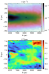 |
Fig. 6. Stellar number count in the plane of galactocentric radius and height, for data sample 2 < MG ≤ 3, averaged over the spatial volume within |Y|< 250 pc. The top panel shows the number count of the GP fit, while the bottom panel shows the ratio with respect to the symmetric analytic fit. The solar position is highlighted with a black plus marker. |
 |
Fig. 7. Phase-space spiral of the immediate solar neighbourhood (Rcyl < 500 pc). The three panels show: (a) the stellar number count density in the (Z, W) phase-space plane; (b) a ratio of this histogram with respect to a best-fit smooth and symmetric background distribution; (c) a ratio with respect to the same background distribution, but projected on the Z-axis. The over-densities at Z ≃ 200 pc and Z ≃ −400 pc have clear counterparts in Fig. 6. In panel b, we exclude regions far from the panel centre, where the total number count is low and the statistical noise is high. In panel c, we mask |Z|< 100 pc, where the Gaia radial velocity sample is dominated by strong selection effects due to stellar crowding. Further details are found in the text. |
Our discussion of number densities in this section has focused on the data sample defined by 2 < MG ≤ 3, which we consider to be most informative. The brighter data samples reach greater distances but it is more difficult to tease out clear stellar number density structures since the information gathered at these distances is plagued by poorer statistics and systematic issues that we have not been able to control for (e.g. degeneracies between dust extinction and distance). Conversely, the dimmest data sample has the greatest number of stars and yields robust and trustworthy results, but also covers a smaller spatial volume. The corresponding plots of these other data samples can be found in Appendix C. Overall, similar stellar number density structures are visible in all four stellar samples, although the perturbations at lower vertical energies are less pronounced for the dimmest data sample.
In Fig. 8 we show the mean vertical velocity distribution for our brightest data sample in the same volume cells that were used in Fig. 5. Because the statistics for the velocity information is poorer, we smoothed these maps in the (X, Y)-plane by convolving it with a 2D Gaussian with a standard deviation of 150 pc in both directions, corresponding to an effective area of 1.4 × 10⁵ pc2. The vertical velocity is offset by 7.25 km s−1 to account for the motion of the Sun with respect to the mid-plane. The corresponding plots for two other data samples can be found in Appendix C, although they are much more limited in distance. The two main stellar number density perturbations in Fig. 5 have clear counterparts in the vertical velocity field. First, the over-density that is close to the Galactic mid-plane at approximately (X, Y) = (−0.3, 0.8) kpc has a vertical velocity counterpart with a similar shape. The feature is seen most clearly in the fourth row of Fig. 8, with negative values for  in the third column, implying compression. Second, the large-scale asymmetries at greater heights have a corresponding structure in the vertical velocity field, as can be seen in the two bottom rows of Fig. 8; towards the Galactic anti-centre, both the north and south have a positive mean vertical velocity. As with the stellar number density perturbation, the feature is present at larger distances from the mid-plane.
 |
Fig. 8. Mean vertical velocities of the data sample with 0 < MG ≤ 1, in the same spatial volumes as in Fig. 5. The results of each bin in z are averaged over a larger area in the (X, Y)-plane for better visibility; the (X, Y)-grid is convolved with a 2D Gaussian with a standard deviation of 150 pc. The two right columns show the number count in the respective spatial volumes; these quantities account for the smoothing in the (X, Y)-plane and correspond to the effective number of stars that inform the |

In Figs. 9 and 10, we show joint contour plots of the stellar number density and vertical velocity perturbations in the spatial region where we saw an elongated perturbation at lower heights, in both n and W. The disk plane area covered in these two figures is determined by the distance limits of the respective data samples, mainly from the  field, which requires vRV measurements; for the same reason, the two dimmer data samples are too limited in distance to be informative of this spatial region. The figures highlight the relation between the two fields. By eye, the perturbations in density and vertical velocity have roughly the same orientation and the same width across the short axis, but they are out of phase by π/2. This general structure is present in both data samples and figures. Simultaneous measurements of a perturbation in n and W allow us to associate a timescale with the disturbance. The continuity equation can be written
 (12)
(12)
 |
Fig. 9. Joint stellar number density perturbation and vertical velocity perturbation in the disk plane, for the data sample with absolute magnitude in 0 < MG ≤ 1, integrated over |z|< 300 pc. The mean vertical velocity distribution is smoothed over 150 pc in X and Y for better visibility. The dotted lines correspond to the location of the Local Spiral Arm, according to Reid et al. (2014). |
 |
Fig. 10. Same as Fig. 9, but for the data sample with absolute magnitude in 1 < MG ≤ 2. The range in X and Y is slightly different in this figure, due to the distance limit imposed by vRV observations. |
which gives the timescale τ = (δn/n)/(ΔW/Δz). The perturbation described here, ΔW ≃ 3 km s−1 for Δz ≃ 600 pc and δn/n ≃ 0.4, which gives τ ≃ 80 Myr. We note that this calculation neglects a stellar source term, which could be significant for the star-forming region of a spiral arm, especially for more luminous stars; this is discussed further in Sect. 6. For a further discussion of the divergence of the local stellar velocity field, see Monari et al. (2015) and Nelson & Widrow (2022).
6. Discussion
The stellar number density and vertical velocity fields show clear evidence for perturbations across our local patch of the disk. The features that we associate with perturbations are present in all four samples, although they differ in amplitude and structure from one sample to the next. For example, the elongated feature centred on (X, Y)≃(−0.3, 0.8) kpc and at heights |z|≲300 pc is most prominent in the brighter samples. We have tentatively identified this feature with the Local Spiral Arm and so the magnitude dependence of the feature may reflect the observation that spiral structure is associated with recent star formation and hence stars at the bright end of the luminosity function (Binney & Merrifield 1998). The general statement is that perturbations in stellar number density n do not perfectly reflect those of the total stellar mass density, although they are clearly related.
To explore the possible connection of this feature with the Local Spiral Arm (Xu et al. 2013), we zoom into this region in Figs. 9 and 10. The n and  perturbations are offset by approximately a quarter wavelength. This suggests a breathing wave that is travelling in the direction of l ≃ 270 deg, roughly coincident with the position of the Local Spiral Arm found by Reid et al. (2014). The link between spiral structure and breathing modes has been established in an analytic study of the linearised Boltzmann equation by Monari et al. (2016a) and in an analysis of high-resolution simulations by Kumar et al. (2022). In a related work, Monari et al. (2016b) showed that a strong Galactic bar can alter and repress the phase offset between the n and
  perturbations; this scenario is disfavoured by our results.
The following toy model illustrates the breathing-mode hypothesis. For simplicity, we assumed that the local gravitational potential is additively separable in R and z and that the vertical component of the potential is harmonic with  . The vertical action-angle variables are then Jz = Ez/Ωz and θz = tan−1(Ωzz/w), where Ez = w2/2 + Φz(z) is the vertical energy. Vertical oscillations follow a clockwise path (i.e. increasing θz) in the (z, w)-plane. For definiteness, we imagine that the unperturbed system is isothermal in the vertical direction so that the equilibrium DF in the (z, w)-plane is
  . The simplest breathing-mode perturbation is proportional to cos(2θz − ωbt). At t = 0, the DF is squeezed in z and stretched in w, thereby increasing the density near the mid-plane. The perturbed DF then rotates in the clockwise sense with a pattern speed ωb/2. The complete model is
![Mathematical equation: $$ \begin{aligned} f(\mathbf{X},W) = f_0(E_z) \{1 + \epsilon E_z\cos [ 2\theta _z - \omega _b t - \chi (X,Y) ] \}, \end{aligned} $$](/articles/aa/full_html/2022/12/aa44453-22/aa44453-22-eq30.gif) (13)
(13)
where χ encodes the propagation of the wave in the plane of the disk. Although this model is purely phenomenological, its functional form is motivated by analytic studies of modes in an isothermal plane (Mathur 1990; Weinberg 1991; Widrow & Bonner 2015).
In Fig. 11 we present a chi-by-eye realisation of the model that captures qualitative features of Figs. 9 and 10. The function χ is chosen to correspond to an outward-propagating, trailing logarithmic spiral:
 (14)
(14)
 |
Fig. 11. Toy model perturbations to the disk. The bottom panel shows n and |

where R and ϕ are galactocentric polar coordinates, p is the tangent of the pitch angle, and the wavelength is 2πR0/k. For the figure, we set k and p so that the wavelength is 1 kpc and the pitch angle is 12°, as is the case for the Local Spiral Arm (Xu et al. 2013). We have also included an envelope function that serves to localise the perturbation about the point (X, Y) = (−200, 600) pc. The three top panels in Fig. 11 correspond to ωbt = {π, 3π/2, 2π}, respectively.
The density and velocity fields of this simple toy model capture the qualitative features seen in the data. However, as discussed in the previous section, the data exhibit a number density perturbation of about 40% and a velocity perturbation of a few km s−1. Our simple toy model predicts stronger perturbation for the velocity field relative to the number density field (where the overall strength is set by the free parameter ϵ). Evidently, an explanation of the observed relative strength of the velocity and density perturbations will require a more complicated model. An obvious extension would be to consider a superposition of modes. Furthermore, as mentioned in the beginning of this section, the observed perturbation in n is likely affected by recent star formation, especially for our brighter data samples. Hence, the over-density in n is likely inflated as compared to the relative over-density of the total matter density field in the same spatial location.
The large-scale bending mode feature is seen as a upward shift in the thicker disk component (roughly |z|> 300 pc), for stars in the direction of the Galactic anti-centre. The same structure is reflected in the vertical velocity distribution, where the corresponding northern and southern spatial volumes have a mean velocity towards the Galactic north, thus having the characteristic of a bending mode. However, the thinner disk component is less affected within the studied range in distance, remaining much more flat for both n and  . The structure can be interpreted as a mix of smaller-scale bending waves and the global Galactic warp as it extends into the solar neighbourhood. This interpretation is consistent with the analysis by Schönrich & Dehnen (2018), who measured
  as a function of Lz (the angular momentum about the z-axis) for the immediate solar neighbourhood stars in the Gaia-TGAS dataset. They found that the variations in
  could be modelled as small-scale oscillations of
  with R (with a wavelength of roughly 2.5 kpc) superimposed on a linear function that increases with R. This linear trend is also consistent with the results from Poggio et al. (2020), who modelled the large-scale Galactic warp and precession of the Milky Way’s stellar disk. In their model, even though the Sun lies just 17 deg from the line of nodes, constant W contours were roughly aligned with Galactic azimuth. We find a similar alignment, as shown in Fig. 8. The situation with n is more complicated. In the model by Poggio et al. (2020), the disk bends toward the south (negative z) in the solar neighbourhood. Thus, we expect that the north–south asymmetry in n should increase with R. Due to our close proximity to the line of nodes, the direction of steepest increase in the asymmetry will be in the direction of increasing R and decreasing ϕ (increasing X and decreasing Y.). This trend is consistent with what we found in Fig. 5 for the regions closest to the mid-plane. However, the sign reverses for greater |z|. This complicated structure in number density is also shown in Fig. 6.
Some structures in n, such as the horizontal bands in the bottom panel of Fig. 6, with |Z| in range 200–600 pc, are projections of the phase-space spiral. The properties of the phase-space spiral such as its phase and amount of winding in the (Z, W)-plane, varies slowly across the disk on scales of a few kiloparsecs in X and Y (e.g. Bland-Hawthorn et al. 2019; Widmark et al. 2021, 2022b; Hunt et al. 2022; also supported by simulations, e.g. Hunt et al. 2021). In Appendix D, we show how the spiral angle in the (Z, W)-plane vary with X and Y, which in turn translates into how the spiral perturbation projects onto the Z-axis. At lower heights (Z ≃ 200 pc), we see a clear correspondence between the spiral density perturbation’s projection in n(Z) and the north-south asymmetries seen in the fourth and fifth panel rows of Fig. 5. Conversely, the two main density perturbations that we have identified in this work, a small-scale breathing mode that we tentatively associate with the Local Spiral Arm and a large-scale bending mode, do not match the properties of a projected phase-space spiral; the first is much too localised in space and is symmetric, and the second is a very large relative perturbation found mainly at greater heights and does not match the azimuthal variation of the phase-space spiral in this spatial region. We refer to Appendix D for further details.
There are likely systematic effects that bias our results, especially at greater distances and in the general direction of the Galactic centre, where dust extinction and stellar crowding are more severe. In principle, there could be some confounding systematic that creates a spatially dependent distance bias, for example arising from dust clouds, which could affect both the n and  fields in the same spatial region. However, this is not likely to explain the two main perturbations that we have identified in this work. For the Local Spiral Arm, the structure in n and
  is elongated and close to the solar position, such that the viewing angle relative to its axis of elongation varies significantly. Despite this, we see a qualitatively similar structure over its axis of elongation. For the large-scale bending mode, its presence at greater heights makes it much less affected by stellar crowding and dust extinction, and we also see it over a large portion of the sky. Furthermore, we see both of these structures in all data samples, at least to the extent that they probe those spatial volumes.
7. Conclusion
We have mapped the stellar number density distribution (n) and the mean vertical velocity distribution ( ), as a function of spatial position in the Milky Way disk, out to a distance of a few kiloparsecs. We have done so in a fairly model-independent manner using GPs, which does not rely on any symmetry assumptions.
In addition to projections of the phase-space spiral, we identify two main perturbation features with respect to a fully symmetric background. First, we see an elongated over-density feature in n and corresponding breathing-mode compression in  at the spatial location of the Local Spiral Arm. The ridges of these n and
  structures are offset in the direction perpendicular to the spiral arm, indicating a travelling breathing mode. Second, we see a large-scale bending mode feature in both n and
  . We make the novel observation that within our studied spatial volume, out to a distance of at least 2 kpc in the direction of the Galactic anti-centre, this bending-mode feature affects the stellar number density at greater heights, while the thinner disk component (|z|≲300 pc) remains more flat in both n and
  .
.
An obvious extension of this work would be to combine a smooth model for the number density field with a model for the full three-dimensional velocity field. This would allow us to use the continuity and Jeans equations to more fully explore the connections between vertical motions and spiral arms as well as other examples of disequilibrium in the disk (Monari et al. 2015, 2016a,b; Nelson & Widrow 2022).
We have demonstrated that with a careful treatment of selection effects, the stellar number density distribution can be mapped even in fairly distant regions of the thin stellar disk. With more sophisticated and accurate complementary distance estimations, using photometric or spectroscopic information, in synergy with improved three-dimensional dust maps, we expect to reach even greater distances and depths in the near future.
Acknowledgments
We would like to thank Friedrich Anders and Giacomo Monari for useful discussions. We also want to thank the anonymous referee for a thorough and constructive report. A.W. acknowledges support from the Carlsberg Foundation via a Semper Ardens grant (CF15-0384). APN is supported by a Research Leadership Award from the Leverhulme Trust. L.M.W. acknowledges the financial support of the Natural Sciences and Engineering Research Council of Canada. This work made use of an HPC facility funded by a grant from VILLUM FONDEN (projectnumber 16599). This work has made use of data from the European Space Agency (ESA) mission Gaia (https://www.cosmos.esa.int/gaia), processed by the Gaia Data Processing and Analysis Consortium (DPAC, https://www.cosmos.esa.int/web/gaia/dpac/consortium). Funding for the DPAC has been provided by national institutions, in particular the institutions participating in the Gaia Multilateral Agreement. This research utilised the following open-source Python packages: MATPLOTLIB (Hunter 2007), NUMPY (Harris et al. 2020), GEORGE (Ambikasaran et al. 2015), HEALPY (Górski et al. 2005).
References
- Ambikasaran, S., Foreman-Mackey, D., Greengard, L., Hogg, D. W., & O’Neil, M. 2015, IEEE Trans. Pattern Anal. Machine Intell., 38, 252 [Google Scholar]
- Anders, F., Khalatyan, A., Queiroz, A. B. A., et al. 2022, A&A, 658, A91 [NASA ADS] [CrossRef] [EDP Sciences] [Google Scholar]
- Antoja, T., Helmi, A., Romero-Gómez, M., et al. 2018, Nature, 561, 360 [Google Scholar]
- Bennett, M., & Bovy, J. 2019, MNRAS, 482, 1417 [NASA ADS] [CrossRef] [Google Scholar]
- Binney, J., & Merrifield, M. 1998, Galactic Astronomy (Princeton University Press) [Google Scholar]
- Bland-Hawthorn, J., Sharma, S., Tepper-Garcia, T., et al. 2019, MNRAS, 486, 1167 [NASA ADS] [CrossRef] [Google Scholar]
- Boubert, D., & Everall, A. 2020, MNRAS, 497, 4246 [NASA ADS] [CrossRef] [Google Scholar]
- Cantat-Gaudin, T., Jordi, C., Vallenari, A., et al. 2018, A&A, 618, A93 [NASA ADS] [CrossRef] [EDP Sciences] [Google Scholar]
- Cantat-Gaudin, T., Fouesneau, M., Rix, H.-W., et al. 2022, A&A, in press, https://doi.org/10.1051/0004-6361/202244784 [Google Scholar]
- Carlin, J. L., DeLaunay, J., Newberg, H. J., et al. 2013, ApJ, 777, L5 [Google Scholar]
- Everall, A., & Boubert, D. 2022, MNRAS, 509, 6205 [Google Scholar]
- Everall, A., Belokurov, V., Evans, N. W., Boubert, D., & Grand, R. J. J. 2022a, MNRAS, 511, 3863 [NASA ADS] [CrossRef] [Google Scholar]
- Everall, A., Evans, N. W., Belokurov, V., Boubert, D., & Grand, R. J. J. 2022b, MNRAS, 511, 2390 [NASA ADS] [CrossRef] [Google Scholar]
- Friske, J. K. S., & Schönrich, R. 2019, MNRAS, 490, 5414 [Google Scholar]
- Gaia Collaboration (Prusti, T., et al.) 2016, A&A, 595, A1 [NASA ADS] [CrossRef] [EDP Sciences] [Google Scholar]
- Gaia Collaboration (Katz, D., et al.) 2018, A&A, 616, A11 [NASA ADS] [CrossRef] [EDP Sciences] [Google Scholar]
- Gaia Collaboration (Drimmel, R., et al.) 2022a, A&A, in press, https://doi.org/10.1051/0004-6361/202243797 [Google Scholar]
- Gaia Collaboration (Vallenari, A., et al.) 2022b, A&A, in presss, https://doi.org/10.1051/0004-6361/202243940 [Google Scholar]
- Górski, K. M., Hivon, E., Banday, A. J., et al. 2005, ApJ, 622, 759 [Google Scholar]
- Harris, C. R., Millman, K. J., van der Walt, S. J., et al. 2020, Nature, 585, 357 [NASA ADS] [CrossRef] [Google Scholar]
- Hunt, J. A. S., Price-Whelan, A. M., Johnston, K. V., & Darragh-Ford, E. 2022, MNRAS, 516, L7 [NASA ADS] [CrossRef] [Google Scholar]
- Hunt, J. A. S., Stelea, I. A., Johnston, K. V., et al. 2021, MNRAS, 508, 1459 [NASA ADS] [CrossRef] [Google Scholar]
- Hunter, J. D. 2007, Comput. Sci. Eng., 9, 90 [NASA ADS] [CrossRef] [Google Scholar]
- Kingma, D. P., & Ba, J. 2014, ArXiv e-prints [arXiv:1412.6980] [Google Scholar]
- Kordopatis, G., Schultheis, M., McMillan, P. J., et al. 2022, A&A, in press, https://doi.org/10.1051/0004-6361/202244283 [Google Scholar]
- Kumar, A., Ghosh, S., Kataria, S. K., Das, M., & Debattista, V. P. 2022, MNRAS, 516, 1114 [NASA ADS] [CrossRef] [Google Scholar]
- Laporte, C. F. P., Minchev, I., Johnston, K. V., & Gómez, F. A. 2019, MNRAS, 485, 3134 [Google Scholar]
- Li, H., & Widrow, L. M. 2021, MNRAS, 503, 1586 [CrossRef] [Google Scholar]
- Martinez-Medina, L., Pérez-Villegas, A., & Peimbert, A. 2022, MNRAS, 512, 1574 [NASA ADS] [CrossRef] [Google Scholar]
- Mathur, S. D. 1990, MNRAS, 243, 529 [NASA ADS] [Google Scholar]
- McMillan, P. J. 2016, MNRAS, 465, 76 [Google Scholar]
- Monari, G., Famaey, B., & Siebert, A. 2015, MNRAS, 452, 747 [NASA ADS] [CrossRef] [Google Scholar]
- Monari, G., Famaey, B., & Siebert, A. 2016a, MNRAS, 457, 2569 [Google Scholar]
- Monari, G., Famaey, B., Siebert, A., et al. 2016b, MNRAS, 461, 3835 [Google Scholar]
- Nelson, P., & Widrow, L. M. 2022, MNRAS, 516, 5429 [NASA ADS] [CrossRef] [Google Scholar]
- Oort, J. H. 1932, Bull. Astron. Inst. Neth., 6, 249 [NASA ADS] [Google Scholar]
- Poggio, E., Drimmel, R., Andrae, R., et al. 2020, Nature Astron., 4, 590 [NASA ADS] [CrossRef] [Google Scholar]
- Rasmussen, C. E., & Williams, C. K. I. 2005, Gaussian Processes for Machine Learning (Adaptive Computation and Machine Learning) (The MIT Press) [Google Scholar]
- Reid, M. J., Menten, K. M., Brunthaler, A., et al. 2014, ApJ, 783, 130 [Google Scholar]
- Reid, M. J., Menten, K. M., Brunthaler, A., et al. 2019, ApJ, 885, 131 [Google Scholar]
- Rybizki, J., Rix, H.-W., Demleitner, M., Bailer-Jones, C. A. L., & Cooper, W. J. 2021, MNRAS, 500, 397 [Google Scholar]
- Schönrich, R., & Dehnen, W. 2018, MNRAS, 478, 3809 [Google Scholar]
- Sellwood, J. A. 2013, in Planets, Stars and Stellar Systems. Volume 5: Galactic Structure and Stellar Populations, eds. T. D. Oswalt, & G. Gilmore, 5, 923 [Google Scholar]
- Titsias, M. 2009, J. Mach. Learn. Res. Proc. Track, 5, 567 [Google Scholar]
- Weinberg, M. D. 1991, ApJ, 373, 391 [NASA ADS] [CrossRef] [Google Scholar]
- Widmark, A., Laporte, C. F. P., de Salas, P. F., & Monari, G. 2021, A&A, 653, A86 [NASA ADS] [CrossRef] [EDP Sciences] [Google Scholar]
- Widmark, A., Hunt, J. A. S., Laporte, C. F. P., & Monari, G. 2022a, A&A, 663, A16 [NASA ADS] [CrossRef] [EDP Sciences] [Google Scholar]
- Widmark, A., Laporte, C. F. P., & Monari, G. 2022b, A&A, 663, A15 [NASA ADS] [CrossRef] [EDP Sciences] [Google Scholar]
- Widrow, L. M., & Bonner, G. 2015, MNRAS, 450, 266 [NASA ADS] [CrossRef] [Google Scholar]
- Widrow, L. M., Gardner, S., Yanny, B., Dodelson, S., & Chen, H.-Y. 2012, ApJ, 750, L41 [Google Scholar]
- Williams, M. E. K., Steinmetz, M., Binney, J., et al. 2013, MNRAS, 436, 101 [Google Scholar]
- Xu, Y., Li, J. J., Reid, M. J., et al. 2013, ApJ, 769, 15 [Google Scholar]
- Xu, Y., Newberg, H. J., Carlin, J. L., et al. 2015, ApJ, 801, 105 [Google Scholar]
- Yanny, B., & Gardner, S. 2013, ApJ, 777, 91 [Google Scholar]
Appendix A: Stellar ages
In Fig. A.1, we show the age distribution for stars within 400 pc of the Sun, which was the same as the distance range used in Fig. 1. The ages were taken from the catalogue by Kordopatis et al. (2022), which were inferred using spectroscopically derived atmospheric parameters in combination with 2MASS and Gaia photometry. The numbers of stars used for the four distributions were 19k, 13k, 74k, and 281k. Thus, this age distribution comes from a small subset of stars observed with Gaia, but nonetheless gives an idea about the age range of our respective data samples.
 |
Fig. A.1. Stellar age distribution for the four absolute magnitude cuts of our data samples based on stars within 400 pc of the Sun. The markers denote the mid-point of age bins with a width of 500 Myr in the range 0–13 Gyr. The vertical axis shows the relative fraction of stars in each bin, normalised such that the area below the curve is unity in these units. |
Appendix B: Symmetric analytic function-fitted parameters
The fitted free parameters of fsymm. can be found in Table B.1. We also performed fits with a smaller or larger number of disk components. Using more than three disk components did not produce noticeably better fits. Using only two disk components did in fact produce some artefacts, because in this case fsymm. could not replicate the heavy tails towards high |Z|. An exception is the very brightest data sample, for which two disk components have practically identical scale length and scale height values, such that only two disk component would suffice. The scale lengths and heights of the three disk components are increasing in unison, for all four data samples. The height of the Sun with respect to the disk mid-plane is found to be roughly 11 pc, with variations of a few parsec between the data samples.
Inferred parameters for fsymm., for our four data samples.
As an additional test, we modified the functional form of fsymm. to read
 (B.1)
(B.1)
This differs from Eq. 11 in that we have added the α and β parameters, which correspond to a potential inclination of the disk mid-plane, different from the plane defined by b = 0 deg in the Gaia catalogue. However, our results for the plane inclination are minimal; we infer (α, β) values of (0.00025, -0.00591), (-0.00001, -0.00612), (0.00176, -0.00725), and (0.00407, -0.00634) for our four data samples. These values mean that at a 2 kpc distance from the Sun, the disk mid-plane varies on the scale of roughly 10 pc as compared to the plane defined by b = 0 deg. We see slight evidence for a misalignment between these two planes, but this result could very well be affected by systematic errors. Either way, this misalignment is not strong enough to alter the general conclusions of this work.
Appendix C: Supplementary figures
In Figs. C.1–C.8, we show plots corresponding to Figs. 5, 6, and 8 in the main text, but for our other data samples (although the velocity plot for our dimmest data sample is excluded due to covering such a small spatial volume). For brighter data samples, in the (X, Y)-plane projections of Figs. C.1 and C.2, as well as the (R, z)-plane projections of Figs. C.4 and C.5, the distant regions (≳2 kpc) seem to suffer from strong systematic errors, especially close to the disk mid-plane.
Appendix D: Spiral angle plots
In Figs. D.1 and D.2, we show how the spiral angle varies in the (X, Y)-plane. The spiral angle, more specifically, is given by the location of the phase-space spiral over-density in the (z, w)-plane along the isocontour of vertical energy. In the two plots, this vertical energy is fixed to either Ez = Φ(200 pc) or Ez = Φ(500 pc). These results come from directly from Widmark et al. (2022b), although this figure was not included in that article; we refer to that article for further details.
 |
Fig. D.1. Angle of the phase-space spiral at the iso-energy contour Ez = Φ(200 pc) in the (z, w)-plane, as inferred in Widmark et al. (2022b). The colour bar is cyclical. If the angle is close to 0 (or 2π, equivalently), then the spiral perturbation corresponds to an over-density at the phase-space coordinates (Z, W) = (200 pc, 0 km s−1); conversely, if the angle is close to π, then the spiral corresponds to an under-density at (Z, W) = (200 pc, 0 km s−1). Area cells that are crossed over in white are marked as less trustworthy; we refer to Widmark et al. (2022b) for details. |
In Fig. D.1 and Ez = Φ(200 pc), an angle close to 0 (or 2π, equivalently), means that the spiral perturbation corresponds to an over-density when projected onto the Z-axis, at the height Z ≃ 200 pc. Because the spiral is single-armed and asymmetric, this also means that there is an under-density in n(Z) at Z ≃ −200 pc. This agrees well with the north-south asymmetry seen in the third and fourth rows of Figs. 5, C.1–C.3, which has a corresponding morphology in the (X, Y)-plane, for example in terms of an over-density region in the direction of positive Y. The projected perturbation of the spiral at greater heights is less clear. The projected spiral density perturbation at Z ≃ 500 pc, as seen in Fig. D.2, does not have a clear counterpart in the fourth or fifth rows of of Fig. 5, indicating a superposition of other significant asymmetries at these greater heights.
It is also evident from these figures that the spiral angle varies significantly with the azimuth over scales of a few kiloparsecs. The morphology of the phase-space spiral therefore does not match the two main perturbation features that we identify in this work (the small-scale breathing mode associated with the Local Spiral Arm, and the large-scale bending mode), whose properties vary on either much smaller or much larger scales in the (X, Y)-plane.
All Tables
All Figures
|
Fig. 1. Colour-magnitude diagram of stars in StarHorse within a distance of 400 pc. The panel on the right side shows the 1D absolute magnitude histogram. The dashed lines correspond to the magnitude cuts of our four data samples. The colour and absolute magnitude values are intrinsic and dust-corrected as given directly by the StarHorse catalogue. |
| In the text | |
|
Fig. 2. Upper distance limit, given by Eq. (4), as a function of angles l and b, for our four data samples. The centre of the map is in the direction of the Galactic centre, while positive b is pointing upwards and positive l is pointing to the right. |
| In the text | |
|
Fig. 3. Stellar number counts per area cell in the (X, Y)-plane, for our four data samples (specified in the top right corners), after masks have been applied. The arrows in the rightmost panel show the direction of the Galactic centre and the direction of Galactic rotation. The axis ranges are shared between all panels. |
| In the text | |
|
Fig. 4. GP fit for data sample with absolute magnitude cuts 2 < MG ≤ 3. Each panel corresponds to a 100-by-100 pc area cell in the (X, Y)-plane, labelled by indices i and j according to Eq. (6), thus centred on (X, Y) = (200, −600) pc. The horizontal and vertical axes show height with respect to the Sun and the normalised stellar number count as defined in Eq. (8). The solid lines correspond to the GP fits, with a smooth shaded region signifying its dispersion (mostly too small to see by eye). The jagged shaded region corresponds to the 1σ band of the data number count. The axis ranges are the same for all panels. |
| In the text | |
|
Fig. 5. Stellar number density variations in the (X, Y)-plane of the data sample with 2 < MG ≤ 3, for different bins in height. The left (middle) column shows the density variations north (south) of the mid-plane as the ratio of the GP and symmetric analytic fit (as described in Sects. 3.3 and 3.4, respectively). The right column shows the asymmetries between the north and south of the GP fits, where each row corresponds to a specific range in height with respect to the mid-plane location when fitting fsymm.. The arrows in the top right panel show the directions of the Galactic centre and Galactic rotation. The axes ranges are shared between all panels. |
| In the text | |
|
Fig. 6. Stellar number count in the plane of galactocentric radius and height, for data sample 2 < MG ≤ 3, averaged over the spatial volume within |Y|< 250 pc. The top panel shows the number count of the GP fit, while the bottom panel shows the ratio with respect to the symmetric analytic fit. The solar position is highlighted with a black plus marker. |
| In the text | |
|
Fig. 7. Phase-space spiral of the immediate solar neighbourhood (Rcyl < 500 pc). The three panels show: (a) the stellar number count density in the (Z, W) phase-space plane; (b) a ratio of this histogram with respect to a best-fit smooth and symmetric background distribution; (c) a ratio with respect to the same background distribution, but projected on the Z-axis. The over-densities at Z ≃ 200 pc and Z ≃ −400 pc have clear counterparts in Fig. 6. In panel b, we exclude regions far from the panel centre, where the total number count is low and the statistical noise is high. In panel c, we mask |Z|< 100 pc, where the Gaia radial velocity sample is dominated by strong selection effects due to stellar crowding. Further details are found in the text. |
| In the text | |
|
Fig. 8. Mean vertical velocities of the data sample with 0 < MG ≤ 1, in the same spatial volumes as in Fig. 5. The results of each bin in z are averaged over a larger area in the (X, Y)-plane for better visibility; the (X, Y)-grid is convolved with a 2D Gaussian with a standard deviation of 150 pc. The two right columns show the number count in the respective spatial volumes; these quantities account for the smoothing in the (X, Y)-plane and correspond to the effective number of stars that inform the |
| In the text | |
|
Fig. 9. Joint stellar number density perturbation and vertical velocity perturbation in the disk plane, for the data sample with absolute magnitude in 0 < MG ≤ 1, integrated over |z|< 300 pc. The mean vertical velocity distribution is smoothed over 150 pc in X and Y for better visibility. The dotted lines correspond to the location of the Local Spiral Arm, according to Reid et al. (2014). |
| In the text | |
|
Fig. 10. Same as Fig. 9, but for the data sample with absolute magnitude in 1 < MG ≤ 2. The range in X and Y is slightly different in this figure, due to the distance limit imposed by vRV observations. |
| In the text | |
|
Fig. 11. Toy model perturbations to the disk. The bottom panel shows n and |
| In the text | |
|
Fig. A.1. Stellar age distribution for the four absolute magnitude cuts of our data samples based on stars within 400 pc of the Sun. The markers denote the mid-point of age bins with a width of 500 Myr in the range 0–13 Gyr. The vertical axis shows the relative fraction of stars in each bin, normalised such that the area below the curve is unity in these units. |
| In the text | |
 |
Fig. C.1. Same as Fig. 5, but for the stellar sample with 0 < MG ≤ 1. |
| In the text | |
 |
Fig. C.2. Same as Fig. 5, but for the stellar sample with 1 < MG ≤ 2. |
| In the text | |
 |
Fig. C.3. Same as Fig. 5, but for the stellar sample with 3 < MG ≤ 4. |
| In the text | |
 |
Fig. C.4. Same as Fig. 6, but for the stellar sample with 0 < MG ≤ 1. |
| In the text | |
 |
Fig. C.5. Same as Fig. 6, but for the stellar sample with 1 < MG ≤ 2. |
| In the text | |
 |
Fig. C.6. Same as Fig. 6, but for the stellar sample with 3 < MG ≤ 4. |
| In the text | |
 |
Fig. C.7. Same as Fig. 8, but for the stellar sample with 1 < MG ≤ 2. |
| In the text | |
 |
Fig. C.8. Same as Fig. 8, but for the stellar sample with 2 < MG ≤ 3. |
| In the text | |
|
Fig. D.1. Angle of the phase-space spiral at the iso-energy contour Ez = Φ(200 pc) in the (z, w)-plane, as inferred in Widmark et al. (2022b). The colour bar is cyclical. If the angle is close to 0 (or 2π, equivalently), then the spiral perturbation corresponds to an over-density at the phase-space coordinates (Z, W) = (200 pc, 0 km s−1); conversely, if the angle is close to π, then the spiral corresponds to an under-density at (Z, W) = (200 pc, 0 km s−1). Area cells that are crossed over in white are marked as less trustworthy; we refer to Widmark et al. (2022b) for details. |
| In the text | |
 |
Fig. D.2. Same as Fig. D.1 but for the iso-energy contour Ez = Φ(500 pc). |
| In the text | |
Current usage metrics show cumulative count of Article Views (full-text article views including HTML views, PDF and ePub downloads, according to the available data) and Abstracts Views on Vision4Press platform.
Data correspond to usage on the plateform after 2015. The current usage metrics is available 48-96 hours after online publication and is updated daily on week days.
Initial download of the metrics may take a while.