| Issue |
A&A
Volume 667, November 2022
|
|
|---|---|---|
| Article Number | L9 | |
| Number of page(s) | 9 | |
| Section | Letters to the Editor | |
| DOI | https://doi.org/10.1051/0004-6361/202244642 | |
| Published online | 11 November 2022 | |
Letter to the Editor
The Great Flare of 2021 November 19 on AD Leonis
Simultaneous XMM-Newton and TESS observations
1
Institut für Astronomie & Astrophysik, Eberhard-Karls-Universität Tübingen, Sand 1, 72076 Tübingen, Germany
e-mail: This email address is being protected from spambots. You need JavaScript enabled to view it.
2
INAF – Osservatorio Astronomico di Palermo, Piazza del Parlamento 1, 90134 Palermo, Italy
3
Dipartimento di Fisica e Chimica, Università degli Studi di Palermo, Piazza del Parlamento 1, 90134 Palermo, Italy
Received:
30
July
2022
Accepted:
13
September
2022
Abstract
We present a detailed analysis of a superflare on the active M dwarf star AD Leonis. The event presents a rare case of a stellar flare that was simultaneously observed in X-rays (with XMM-Newton) and in the optical (with the Transiting Exoplanet Survey Satellite, TESS). The radiated energy in the 0.2 − 12 keV X-ray band (1.26 ± 0.01 × 1033 erg) and the bolometric value (EF, bol = 5.57 ± 0.03 × 1033 erg) place this event at the lower end of the superflare class. The exceptional photon statistics deriving from the proximity of AD Leo has enabled measurements in the 1 − 8 Å GOES band for the peak flux (X1445 class) and integrated energy (EF, GOES = 4.30 ± 0.05 × 1032 erg), which enables a direct comparison with data on flares from our Sun. From extrapolations of empirical relations for solar flares, we estimate that a proton flux of at least 105 cm−2 s−1 sr−1 accompanied the radiative output. With a time lag of 300 s between the peak of the TESS white-light flare and the GOES band flare peak as well as a clear Neupert effect, this event follows the standard (solar) flare scenario very closely. Time-resolved spectroscopy during the X-ray flare reveals, in addition to the time evolution of plasma temperature and emission measure, a temporary increase in electron density and elemental abundances, and a loop that extends into the corona by 13% of the stellar radius (4 × 109 cm). Independent estimates of the footprint area of the flare from TESS and XMM-Newton data suggest a high temperature of the optical flare (25 000 K), but we consider it more likely that the optical and X-ray flare areas represent physically distinct regions in the atmosphere of AD Leo.
Key words: stars: flare / stars: activity / stars: rotation / stars: coronae / stars: individual: AD Leo / X-rays: stars
© B. Stelzer et al. 2022
 Open Access article, published by EDP Sciences, under the terms of the Creative Commons Attribution License (https://creativecommons.org/licenses/by/4.0), which permits unrestricted use, distribution, and reproduction in any medium, provided the original work is properly cited.
This article is published in open access under the Subscribe-to-Open model. This email address is being protected from spambots. You need JavaScript enabled to view it. to support open access publication.
1. Introduction
Contemporaneous multiwavelength data during flares are crucial for understanding the physics of the flare process. Prominent characteristics expected from the standard solar flare scenario (the so-called CSHKP model) include a time lag between diagnostics for the impulsive and the gradual phase (see, e.g., Benz 2002) and a relation between nonthermal and thermal emission, the so-called Neupert effect (Neupert 1968), which was occasionally observed in large stellar flares as a correspondence between the profile of the radio luminosity and the time-derivative of the X-ray luminosity (e.g., Güdel et al. 2002; Osten et al. 2007).
Stellar flares are also known to be a major driver for the evolution of planet atmospheres (e.g., Owen et al. 2020). However, most exoplanet systems are too distant for a detailed characterization of the high-energy (X-ray and UV) emission of the host star. Therefore, models for the effects of stellar irradiation on planets are often based on the observed properties of individual well-known flare stars. Most notably, a prototypical flare on AD Leo, the so-called ‘Great Flare of 1985’ (Hawley & Pettersen 1991), has been the basis for seminal work on the impact of stellar variability on planetary chemistry (Segura et al. 2010; Tilley et al. 2019).
AD Leo is an M-type main-sequence star (SpT M3.5) at a distance of 4.966 ± 0.002 pc (Gaia Collaboration 2020). It has an effective temperature of Teff = 3414 ± 100 K and a radius of R* = 0.426 ± 0.049 R⊙ (Houdebine et al. 2016). Its rotation period of  d (measured on the MOST light curve; Hunt-Walker et al. 2012) and its X-ray luminosity of log LX [erg s−1] = 28.8 (Robrade & Schmitt 2005) place the star in the saturated regime of the rotation-activity relation, where the X-ray emission level does not depend on rotation. For M dwarfs, the spin-down and associated diminishing of activity last up to ∼1 Gyr (Magaudda et al. 2020; Johnstone et al. 2021). Therefore it is difficult to place an age constraint on AD Leo. While it appears to be a typical M dwarf star based on its rotation and X-ray emission level, it is certainly one of the most frequently studied stars in the northern hemisphere.
Its extraordinary brightness originates in its favorable sky position. It has caused AD Leo to become the prototype for M-type dwarf stars, which account for ∼75% of the stars in the Galaxy (e.g., Chabrier 2001). The number of planets known to orbit such stars has been estimated to be very high, especially for low-mass planets, which are the most suitable candidates for being habitable (Dressing & Charbonneau 2013; Sabotta et al. 2021). An entire space mission is dedicated to the discovery of planets around M dwarfs, the Transiting Exoplanet Survey Satellite (TESS; Ricker et al. 2014).
Using the observed UV spectrum of the 1985 AD Leo flare, Venot et al. (2016) simulated the effect of stellar flares onto exoplanet spectra and found that the stellar flare radiation can induce irreversible changes in the chemical composition of hot planets; see also Chen et al. (2021). The X-ray component of the flare was not considered in these studies as no contemporaneous data were taken in that energy band for the 1985 flare of AD Leo. However, X-ray photons penetrate deeper into the planetary atmosphere and have been shown to drive ionization and chemistry in gaseous exoplanets at layers inaccessible to UV radiation (see Locci et al. 2022, and references therein). AD Leo itself has been reported from a radial velocity study to host a hot-Jupiter planet (Tuomi et al. 2018), but the signal was later attributed to stellar activity (Carleo et al. 2020).
The studies discussed above have pointed out the importance of considering that flares are repetitive events. However, flare rates are poorly constrained in the crucial high-energy XUV band. While the planet transit search satellites Kepler and TESS have provided high-quality optical light curves for numerous flare stars, no instruments are available that are suitable for a systematic monitoring of X-ray and UV flares. This also hampers the full characterization of the dynamics and energy output of flares, which requires their simultaneous detection in different wavebands. That this is a difficult task can be assessed from the study of Namekata et al. (2020), for example, which was dedicated to optical and X-ray monitoring of AD Leo. In 8.5 observation nights, only one small flare was observed jointly in X-rays with NICER (Arzoumanian et al. 2014) and optical instruments.
This article is dedicated to the characterization of a large flare on AD Leo that was observed during a recent pointing of the X-ray satellite XMM-Newton. We detected the optical counterpart of this flare in the TESS light curve. In both wavebands the flare energy is above 1033 erg, the lower bound for the radiative energy release that defines a socalled superflare (Schaefer et al. 2000).
2. Analysis of the superflare
On November 18/19, 2021, AD Leo was observed for 86 ks with XMM-Newton through Director’s Discretionary Time. Due to the proximity of the bright star γ Leo (V = 1.98 mag), located about 4.8′ southeast of AD Leo, the X-ray pointing was performed in SMALL WINDOW MODE for the prime instrument EPIC, and the Optical Monitor had to be kept in closed position. The data reduction for EPIC/pn has been carried out with a standard procedure that is described in Appendix A.
The roughly one-day-long XMM-Newton observation is fully covered with TESS Sector 45, which covered the time span from November 6 to December 2, 2021. The most evident feature is a huge flare toward the end of the XMM-Newton exposure, which has a counterpart in the TESS data. The optical flare is barely visible in the TESS PDCSAP light curve and in the averaged target pixel file (TPF) available at the Barbara A. Mikulski Archive for Space Telescopes (MAST) Portal because of the high noise level induced by γ Leo. We therefore had to perform a customized data reduction (explained in Appendix B) to reduce the noise.
In Fig. 1 we present the simultaneous X-ray and optical light curves of the superflare together with the time derivative of the X-ray luminosity. In the remainder of this section, we describe how we extracted physical parameters from the X-ray and optical data of the flare.
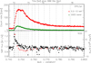 |
Fig. 1. Light curves of the superflare. Top panel: XMM-Newton EPIC/pn count rate in 0.2 − 12 keV (red) and in the GOES band (1.5 − 12.4 keV; green). The binning adapted to the TESS light curve in FAST cadence (20 s) is shown in the bottom panel (black circles), where it is overlaid with the time derivative of the X-ray luminosity (open diamonds). The thick dashed vertical line marks the time of the peak of the flare flux in the TESS light curve, and the dash-dotted lines mark the boundaries of the intervals used for the time-resolved spectral analysis of the X-ray data. For a better display of the main flare phase, a cut has been set to the abscissa values such that the tail of the flare is not shown. |
2.1. X-ray data
The time profile of the X-ray flare is shown in the top panel of Fig. 1 for the broad XMM-Newton energy band (0.2 − 12 keV) and for the GOES band (1 − 8 Å). In the XMM-Newton broad band, it displays a roughly linear (about 340 s long) rise phase, followed by a plateau (lasting about 400 s). The subsequent decay can be described by an exponential followed by a linear phase. We determined the transition between the exponential and the linear phase by fitting a decaying exponential function to the decreasing part of the light curve, starting with the first four bins after the end of the peak phase and successively adding data points until the minimum of  was reached. In this way we determine the exponential decay timescale to τexp = 724 ± 8 s. The subsequent linear phase lasts for the remaining roughly 6 ks until the end of the observation.
At the end of the observation, the count rate was still above the preflare level, suggesting that the underlying quiescent corona changed slightly during the flare. Despite this prolonged tail, the initial fast decay of the X-ray light curve indicates a short-duration event, hence likely occurring in a compact coronal structure.
2.1.1. X-ray spectral analysis
We divided the flare from the start of its rise (2021-11-19 05:48:50.816 UTC) to the end of the exponential phase (2021-11-19 07:08:50.816 UTC) into time intervals of about 10 000 EPIC/pn counts each. The 17 time bins obtained this way have different duration, but roughly the same photon statistics. We extracted an EPIC/pn spectrum from each of the 17 intervals and subtracted the out-of-time events.
Our goal of constraining the physical conditions in the corona of AD Leo during the flare requires an accurate assessment of the underlying quiescent, that is, nonflaring, X-ray emission. To this end, we identified all flare-free parts of the EPIC/pn light curve and combined them into one spectrum. We used this quiescent spectrum as background for the study of the spectral evolution during the X-ray flare. In this way, we obtained a series of flare-only spectra.
The spectrum of each of the 17 individual time slices of the flare was fitted in XSPEC v 12.11.1 (Arnaud 1996) with a two-temperature VAPEC model. To avoid an excessive number of free parameters, we tied the abundances of all elements (X) to that of iron according to the ratio AX/AFe determined for the quiescent state. The remaining elements considered in VAPEC (He, Ca, Al, and Ni), which have no significant emission lines in the spectral range examined, were fixed to the solar values. Because low-resolution X-ray spectra are notoriously affected by degeneracies between abundances and emission measure (EM), we derived the abundances of the quiescent emission of AD Leo from the high-resolution RGS spectrum that was extracted from the same time intervals as the quiescent EPIC/pn spectrum. We used the APED database (Smith et al. 2001) and the updated solar abundance table of Asplund et al. (2009). The full EM distribution analysis of the RGS data will be explained elsewhere. In Table C.1 we report the abundances obtained from the quiescent RGS spectrum because their ratios were used to restrict the spectral model for the flare state, as explained above. Free fit parameters for the 17 EPIC/pn flare spectra were thus the two temperatures and two EM and the abundance of Fe. The best-fit results are listed in Table C.2, where we also report the EM-weighted average temperature and the total EM for each time interval.
The resulting time evolution of the spectral parameters during the flare (EM-weighted average temperature T, sum of the EM of the two components EMtot, and iron abundance) is shown in Fig. 2. By definition of the spectral model, the variation of Fe includes the variation of the abundances of the other elements. Figure 2 shows that in the tail of the exponential decay phase, the flare Fe abundance falls below the quiescent value. This likely indicates a change of the underlying quiescent corona that is manifest also in the elevated count rate after the flare (see Fig. 1). This will be investigated in a future work.
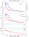 |
Fig. 2. Time evolution throughout the superflare for parameters derived from the XMM-Newton and TESS data. Upper panel: flaring plasma temperature and EM. Middle panel: flaring plasma abundances and electron density. The abundances of all elements are tied to the Fe abundance using the ratios determined for the quiescent state from the RGS spectrum that are listed in Table C.1. Lower panel: thermal energy in the flaring plasma, compared with the total radiated energy in the X-ray and optical bands. |
The top panel of Fig. 2 shows that the peak temperature is reached before the peak of the EM, as expected if the enhanced X-ray radiation is caused by a heating event. Second, the temperature rapidly drops at nearly constant EM (the plateau at the maximum in the light curve). At the onset of the decrease of the EM, the temperature has already decayed to about half its peak value.
Integrating over the fluxes in the 17 time slices, we determined the flare energy. For the GOES band, we found (4.30 ± 0.05) × 1032 erg (see also Table 1), and for the XMM-Newton X-ray band (0.2 − 12 keV), we found EF, XMM = (1.26 ± 0.01) × 1033 erg.
Parameters of the superflare extracted from the optical and X-ray light curves.
2.1.2. Physical conditions of the X-ray flare
The time-resolved spectroscopy during the flare decay can be used to determine the semi-length, L, of the flaring loop, making use of the prescription of Reale et al. (1997), who have performed hydrodynamic simulations to predict the X-ray spectral signature of decaying flare loops. Assuming that the flaring structure has a constant volume (V) with a uniform cross section (S) and that the loop has a half-torus shape (hence its volume is V = 2 ⋅ S ⋅ L), we can infer its semi-length by inspecting the evolution of plasma temperature and density during the decay phase. The hypothesis of constant volume implies that the plasma density, n, is proportional to  . The slope, ζ, of the trajectory traced by the flaring plasma in the log T versus log n space, shown in Fig. 3, then allows us to infer the amount of heat released into the loop during the decay. Combining this with the observed exponential decay time inferred from the light curve (724 ± 8 s) and the temperature at the peak of the flare (log Tpeak = 7.57 ± 0.05 K), we can estimate the loop semi-length. After the first rapid temperature decay at constant EM, the log T vs. log n evolution first displays a joint decrease of both quantities, followed by a minor reheating event. In the first phase of the decay (red points in Fig. 3), the flaring emission is still significantly higher than that of the background corona. This means that the inferred quantities are not significantly affected by the changes occurring in the underlying corona, which is not accounted for in our analysis. We therefore inferred the slope ζ by fitting only the first decay phase, and we obtained ζ = 0.8 ± 0.6. We note, however, that when the whole decay path is included in the fit (blue points and blue line in Fig. 3), a slope of 0.4 ± 0.2 is obtained, which is comprised within the errors in the value obtained for the reduced time-span. The loop semi-length obtained with the equations of Reale et al. (2004), where the procedure calibrated for the EPIC/pn detector was derived, is then L ≈ 4 × 109 cm. The equation that yields the loop length was derived by Reale et al. (1997) under a series of assumptions involving the loop geometry (see the beginning of this section) and heating (exponentially decaying). Therefore, the value of L and all other quantities we derive in the following from this parameter are order-of-magnitude estimates.
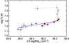 |
Fig. 3. Time evolution of the mean temperature and EM associated with the flare. The red line represents a linear least-squares fit to this first phase of the flare decay (when the flaring emission is still much higher than the slightly variable background corona). The blue line is the fit to the whole exponential decay. |
If the plasma density is known, combining it with the loop length the volume and cross-section of the flaring loop can be determined from the assumptions on the geometry and the definition of the EM. The electron density can be estimated from the high-resolution RGS spectrum, making use of the ratio of forbidden and intercombination lines of He-like triplets (Gabriel & Jordan 1969). To this end, we extracted an RGS spectrum considering the entire exponential flare duration (i.e., the time span that encompasses all the 17 intervals used for the EPIC/pn time-resolved analysis). Details on the RGS analysis will be provided in a forthcoming paper. For the purpose of the current work, we subtracted the RGS spectrum of the quiescent phase from the RGS flare spectrum to inspect the strongest triplets, those of O VII and Ne IX. The significant emission observed in the triplets for this net flare-phase RGS spectrum confirms that even if their formation temperatures are quite low (∼2 and ∼4 MK respectively), the flaring plasma significantly contributes to the emission in these lines. The O VII and Ne IX triplets indicate electron densities ne of  and
and  cm−3. To evaluate the geometric loop parameters, we considered the ne value of 8 × 1011 cm−3 because the higher formation temperature of Ne IX suggests that it probes the flaring plasma density better than the cooler O VII. By averaging the EMtot values of the 17 time intervals we find the total EM of the entire flare, (1.83 ± 0.03) × 1052 cm−3. Combining the electron density with this value and with the loop semi-length, and assuming nH/ne = 0.83 (proper for typical coronal temperatures and chemical compositions), we derive a volume of 3 × 1028 cm3 and a cross section S ≈ 5 × 1018 cm2 for the flaring loop.
After estimating the loop volume together with the detailed evolution of its T and EMtot during the flare, we have the unique opportunity of probing the physical conditions of the flaring plasma during the flare evolution. First, we can infer the evolution of the flaring plasma density ne, obtained as 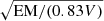 (Fig. 2, middle panel). We can also compute the evolution of the total thermal energy Eth = (3/2)(ne + nH) VkBT of the flaring plasma (Fig. 2, lower panel). In addition, the knowledge of plasma density and temperature allows us to probe the pressure experienced by the flaring plasma, that is, Pgas = (ne + nH)kBT. Because this plasma is magnetically confined, the highest value of Pgas provides a lower limit for the magnetic pressure, Pmag, min = B2/(8π), which in turn implies a minimum magnetic field strength (B) of 500 G and a minimum magnetic energy for the flaring loop of Emag, min = Pmag, min ⋅ V = 4 × 1032 erg (also plotted in the lower panel of Fig. 2).
2.2. Optical data
We searched for the rotational signal and for flares in the TESS light curve. Hereby, we followed our previous work, Stelzer et al. (2016) and Raetz et al. (2020), on data from the K2 mission, and Magaudda et al. (2022, period search adapted for TESS data) and Stelzer et al. (2022, flare search on TESS data).
2.2.1. Analysis of the rotation signal
A detailed description and a graphical illustration of our period search on AD Leo can be found in Appendix D. We found a rotation period of 2.194 ± 0.004, which is consistent with the period found by Hunt-Walker et al. (2012). The half-amplitude of the rotation signal is 0.00217 ± 0.00007. We estimated the spot coverage of AD Leo using the relations given by Notsu et al. (2019). With their Eq. (4), which they deduced from Berdyugina (2005), the spot temperature, Tspot, was computed from AD Leo’s effective temperature. With the computed value of Tspot = 2955 K, we found with Eq. (3) of Notsu et al. (2019) a spot filling factor of Aspot/Astar ≈ 1.0%, where Aspot is the spotted area and Astar is the total surface area of the star.
2.2.2. Flare analysis
We validated four flare candidates in the full light curves. They include the X-ray superflare that was clearly detected in the TESS light curve (see the bottom panel of Fig. 1). In Table 1 we provide all relevant flare properties for the superflare determined by our algorithm, namely the duration (Δt, the time between the first and last flare point), the relative peak flare amplitude (Apeak, the continuum flux level subtracted from the flux of the peak), the absolute peak flare amplitude (ΔL, multiplying Apeak by the quiescent stellar luminosity), and the equivalent duration (ED, integral under the flare). Following Davenport (2016), we calculated the flare energy, EF, by multiplying the ED with the quiescent stellar luminosity of AD Leo in the TESS band, which we determined from the TESS magnitude of AD Leo (T = 7.036) to be Lqui, T = 2.4 × 1031 erg s−1. This value is consistent within 5% with the luminosity that we obtain when we use AD Leo’s effective temperature and radius and integrate the blackbody function taking the TESS filter transmission into account. Assuming for the optical flare a blackbody emission at a constant temperature of 9000 K (as is typically observed for solar White-Light Flares, WLFs, Kretzschmar 2011), we can constrain the emitting area (assumed to be variable) to match the observed amplitude of the TESS light curve, LF, T(t)/Lqui, T. We found a maximum value for the area of 8.4 × 1019 cm2. Multiplying this by the flare surface flux yields the bolometric flare luminosity (LF, bol = 3.1 × 1031 erg s−1), and integration over the flare light curve gives the bolometric energy radiated by the flare (EF, bol = (5.57 ± 0.03) × 1033 erg).
3. Discussion
The energy of the November 2021 flare on AD Leo exceeds the canonical threshold for a superflare, 1033 erg, in both the TESS and the XMM-Newton band. It was stronger by a factor 30 than the largest solar flare observed to date, the Sepember 1859 Carrington event, which was of GOES class X45 (Hudson 2021), while for the AD Leo superflare, we measure a peak flux in the 1 − 8 Å band of (1.38 ± 0.03) × 10−10 erg cm−2 s−1, corresponding to an X1445 event on the GOES flux scale. It is a small event when compared with the largest superflares reported from main-sequence stars in the optical band, however (e.g., Schaefer et al. 2000; Maehara et al. 2012). In X-rays, on the other hand, observations of giant flares have mostly been limited to pre-main-sequence objects or interacting binaries (e.g., Preibisch et al. 1995; Grosso et al. 1997; Pandey & Singh 2012; Getman & Feigelson 2021).
The time profile of the event on AD Leo in November 2021 is similar to the profile of a standard solar flare, where optical emission, associated with the energy deposited by nonthermal high-energy particles in the lower layers of the stellar atmosphere, precedes the X-ray emission peak because of the subsequent chromospheric evaporation (see, e.g., Castellanos Durán & Kleint 2020). The brightness peak in the optical is observed about 300 s before the X-ray maximum in the GOES band. The optical light curve is strongly peaked, while the X-ray maximum is a plateau that transitions into an exponential decay, followed by a slow linear decrease. The chromospheric evaporation scenario (see, e.g., Benz 2017) is further corroborated by the increase in density and elemental abundances that is observed during the flare, which also provides new constraints on the metal depletion in coronal plasma. The higher abundance of the flaring (Fe/Fe⊙ ∼ 0.9) compared to the quiescent plasma (Fe/Fe⊙ ∼ 0.3) clearly proves that the quiescent corona is metal depleted with respect to the chromospheric material, which shows its higher metallicity in the X-rays during the initial phases of the flare. For the first time, we constrained the timescales of coronal metal depletion through the rapid decrease (in a few 100 s) in the elemental abundances after the chromospheric evaporation event.
In absence of data in the radio band, the WLF seen with TESS can be taken as a proxy for the nonthermal component because in the standard flare scenario (e.g., Benz 2017), it is produced by the bombardment of lower atmospheric layers with (nonthermal) electrons from the magnetic reconnection site. We have calculated the evolution of the time derivative of LX, shown as open diamonds in the bottom panel of Fig. 1, from the fluxes measured in the 17 time bins representing the exponential flare phase. The behavior follows that of the WLF, demonstrating the presence of the Neupert effect.
The TESS and XMM-Newton data have provided independent estimates for the surface coverage of the flare footprint. The time-averaged area of the optical flare, determined from the changing amplitude of the TESS light curve, is larger than the X-ray based area by about a factor of seven. A temperature of 25 000 K for the optical flare would reconcile this discrepancy. However, it is likely that the two measurements probe different emitting regions. The X-ray emission, produced by optically thin plasma, provides the cross-section of the coronal part of the loop, while the optical emission originates from the optically thick lower layers of the flaring structure. Hence, the area inferred from the optical flare might embrace both the horizontal extent and vertical structuring of the flaring loop footpoints. The TESS light curve displays a fairly regular sine-like rotational modulation (Fig. D.1). This means that at the epoch of the observation, AD Leo’s photosphere may have been dominated by a single spot group. The flare occurred at phase 0.78 of the rotational signal, with phase 0.0 corresponding to the minimum flux. This means the flare took place when the spotted part of the photosphere was located near the limb. If the flare was indeed spatially connected to the spot, as is typically seen in solar flares (e.g., Toriumi & Wang 2019), we had a lateral view onto the loop structure. We speculate that in such a geometry, the high observed flare area inferred from the TESS data can be accounted for if the optical flare region had a significant vertical extent.
Figure 4 shows that the AD Leo superflare is consistent with the extrapolation of the power-law relation between white-light energy and GOES peak flux derived for the solar flare sample of Namekata et al. (2017). The inclusion of AD Leo increases the range of values by several orders of magnitude, and allows, in contrary to Namekata et al.’s study, which was based solely on solar flares, to constrain the power-law relation.
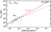 |
Fig. 4. Empirical relation of WLF energy and GOES flux for solar flares and power-law fits performed by Namekata et al. (2017) on them using a linear regression method and a linear regression bisector method (solid and dashed lines). The red line is our fit including the AD Leo superflare, which yields in the double logarithmic form (log EWLF = a + b ⋅ log FGOES), a slope b = 1.150 ± 0.005, and an axis-offset of a = 34.711 ± 0.007, where the uncertainties are the standard deviations of the fit. |
In the empirical relation of flare duration (tF) and energy (EF), the AD Leo WLF is placed among the smallest Kepler superflares on solar-type (i.e., G-type main-sequence) stars observed with similar cadence, that is, Kepler one-minute light curves (Namekata et al. 2017). The theoretical scaling laws presented by these authors predict the magnetic field strength and coronal loop length for a given tF and EF. For AD Leo, B ∼ 100 − 200 G is found, which is somewhat lower than the value we measured from the X-ray data (Bmin ≈ 500 G). This is consistent with the finding by Namekata et al. (2017) who showed by comparison to resolved solar flares that the scaling laws underpredict the field strength. The loop length obtained for the AD Leo superflare from the scaling laws is ≈1010 cm, which is about a factor two larger than the value derived from the X-ray analysis.
The energetic particle flux that reaches the planet (see, e.g., Tilley et al. 2019) is of the utmost importance for evaluating the impact of stellar flares on planets. For the Sun-Earth system, calibrations between the flux of protons with energy > 10 MeV (Ip) and the X-ray flux in the GOES band at the flare peak were recently updated by Herbst et al. (2019). We estimate a proton flux of Ip ∼ 0.1 × 106 cm−2 s−1 sr−1 (from Eq. (4) of Herbst et al. (2019)) and Ip ∼ 20.1 × 106 cm−2 s−1 sr−1 (from their Eq. (5)) for the X-ray superflare of AD Leo. An even larger possible range is obtained when the uncertainties of the solar empirical relations are folded in. Herbst et al. (2019) presented several stellar flares overlaid on the extrapolated solar relation between Ip and GOES flux, including Kepler superflares, and UV events on some benchmark M dwarfs. However, we stress that none of these events has an actual measurement of the X-ray peak flux, and the GOES class for all of them has been estimated using empirical relations to transform observed fluxes at lower wavelengths into the X-ray band, which introduces significant additional uncertainties.
4. Conclusions
The high-cadence simultaneous coverage throughout the full event in the optical and X-ray band makes this superflare on AD Leo a special calibrator for stellar flare physics and the stellar input to exoplanet atmospheres. The exceptionelly good signal at high energies enables evaluating the flare energetics in the GOES band, which provides the rare possibility of quantifying the relation of stellar X-ray superflares and the much larger data base of solar flares. The AD Leo flare exceeds the largest solar flare, the Carrington event, by a factor of 30 in peak X-ray flux and by a factor of 14 in energy. Stellar flares with energies up to about 1037 erg have been reported in the literature. However, in most cases, the radiative output in the X-ray band was estimated from empirical relations with optical or UV flare diagnostics, which are subject to order-of-magnitude uncertainties. The parameters inferred in such an indirect way are correspondingly ill determined. With its simultaneous WLF and GOES band measurements, we were able to verify that the energetics of the AD Leo flare, and therefore likely that of other stellar superflares, constitute a scaled-up version of solar flares. We also derived the soft proton flux that is expected to be associated with the event, which may be helpful for future exoplanet studies.
Fortran Version v2.3.01, released 2011-09-13 by Mathias Zechmeister
Acknowledgments
We wish to thank the anonymous referee. M. Caramazza is supported by the Bundesministerium für Wirtschaft und Energie through the Deutsches Zentrum für Luft- und Raumfahrt e.V. (DLR) under grant number FKZ 50 OR 2105. This research made use of observations obtained with XMM-Newton, an ESA science mission with instruments and contributions directly funded by ESA Member States and NASA. This paper includes data collected by the TESS mission, which are publicly available from the Mikulski Archive for Space Telescopes (MAST). Funding for the TESS mission is provided by NASA’s Science Mission directorate.
References
- Arnaud, K. A. 1996, in Astronomical Data Analysis Software and Systems V, eds. G. H. Jacoby, & J. Barnes, ASP Conf. Ser., 101, 17 [NASA ADS] [Google Scholar]
- Arzoumanian, Z., Gendreau, K. C., Baker, C. L., et al. 2014, in Space Telescopes and Instrumentation 2014: Ultraviolet to Gamma Ray, eds. T. Takahashi, J. W. A. den Herder, & M. Bautz, SPIE Conf. Ser., 9144, 914420 [NASA ADS] [Google Scholar]
- Asplund, M., Grevesse, N., Sauval, A. J., & Scott, P. 2009, ARA&A, 47, 481 [NASA ADS] [CrossRef] [Google Scholar]
- Benz, A. 2002, Plasma Astrophysics, 2nd edn. (Dordrecht: Kluwer Academic Publishers), 279 [Google Scholar]
- Benz, A. O. 2017, Liv. Rev. Sol. Phys., 14, 2 [Google Scholar]
- Berdyugina, S. V. 2005, Liv. Rev. Sol. Phys., 2, 8 [Google Scholar]
- Carleo, I., Malavolta, L., Lanza, A. F., et al. 2020, A&A, 638, A5 [NASA ADS] [CrossRef] [EDP Sciences] [Google Scholar]
- Castellanos Durán, J. S., & Kleint, L. 2020, ApJ, 904, 96 [CrossRef] [Google Scholar]
- Chabrier, G. 2001, ApJ, 554, 1274 [NASA ADS] [CrossRef] [Google Scholar]
- Chen, H., Zhan, Z., Youngblood, A., et al. 2021, Nat. Astron., 5, 298 [Google Scholar]
- Davenport, J. R. A. 2016, ApJ, 829, 23 [Google Scholar]
- Dressing, C. D., & Charbonneau, D. 2013, ApJ, 767, 95 [Google Scholar]
- Gabriel, A. H., & Jordan, C. 1969, MNRAS, 145, 241 [Google Scholar]
- Gaia Collaboration 2020, VizieR Online Data Catalog: I/350 [Google Scholar]
- Getman, K. V., & Feigelson, E. D. 2021, ApJ, 916, 32 [NASA ADS] [CrossRef] [Google Scholar]
- Gilliland, R. L., & Fisher, R. 1985, PASP, 97, 285 [CrossRef] [Google Scholar]
- Grosso, N., Montmerle, T., Feigelson, E. D., et al. 1997, Nature, 387, 56 [NASA ADS] [CrossRef] [Google Scholar]
- Güdel, M., Audard, M., Smith, K. W., et al. 2002, ApJ, 577, 371 [CrossRef] [Google Scholar]
- Hawley, S. L., & Pettersen, B. R. 1991, ApJ, 378, 725 [Google Scholar]
- Herbst, K., Papaioannou, A., Banjac, S., & Heber, B. 2019, A&A, 621, A67 [NASA ADS] [CrossRef] [EDP Sciences] [Google Scholar]
- Houdebine, E. R., Mullan, D. J., Paletou, F., & Gebran, M. 2016, ApJ, 822, 97 [NASA ADS] [CrossRef] [Google Scholar]
- Hudson, H. S. 2021, ARA&A, 59 [Google Scholar]
- Hunt-Walker, N. M., Hilton, E. J., Kowalski, A. F., Hawley, S. L., & Matthews, J. M. 2012, PASP, 124, 545 [NASA ADS] [CrossRef] [Google Scholar]
- Johnstone, C. P., Bartel, M., & Güdel, M. 2021, A&A, 649, A96 [EDP Sciences] [Google Scholar]
- Kretzschmar, M. 2011, A&A, 530, A84 [NASA ADS] [CrossRef] [EDP Sciences] [Google Scholar]
- Locci, D., Petralia, A., Micela, G., et al. 2022, PSJ, 3, 1 [NASA ADS] [Google Scholar]
- Maehara, H., Shibayama, T., Notsu, S., et al. 2012, Nature, 485, 478 [NASA ADS] [Google Scholar]
- Magaudda, E., Stelzer, B., Covey, K. R., et al. 2020, A&A, 638, A20 [NASA ADS] [CrossRef] [EDP Sciences] [Google Scholar]
- Magaudda, E., Stelzer, B., Raetz, S., et al. 2022, A&A, 661, A29 [NASA ADS] [CrossRef] [EDP Sciences] [Google Scholar]
- Namekata, K., Sakaue, T., Watanabe, K., et al. 2017, ApJ, 851, 91 [Google Scholar]
- Namekata, K., Maehara, H., Sasaki, R., et al. 2020, PASJ, 72, 68 [NASA ADS] [CrossRef] [Google Scholar]
- Neupert, W. M. 1968, ApJ, 153, L59 [NASA ADS] [CrossRef] [Google Scholar]
- Notsu, Y., Maehara, H., Honda, S., et al. 2019, ApJ, 876, 58 [Google Scholar]
- Osten, R. A., Drake, S., Tueller, J., et al. 2007, ApJ, 654, 1052 [NASA ADS] [CrossRef] [Google Scholar]
- Owen, J. E., Shaikhislamov, I. F., Lammer, H., Fossati, L., & Khodachenko, M. L. 2020, Space Sci. Rev., 216, 129 [Google Scholar]
- Pandey, J. C., & Singh, K. P. 2012, MNRAS, 419, 1219 [NASA ADS] [CrossRef] [Google Scholar]
- Preibisch, T., Neuhaeuser, R., & Alcala, J. M. 1995, A&A, 304, L13 [NASA ADS] [Google Scholar]
- Raetz, S., Stelzer, B., Damasso, M., & Scholz, A. 2020, A&A, 637, A22 [NASA ADS] [CrossRef] [EDP Sciences] [Google Scholar]
- Reale, F., Micela, G., Peres, G., Betta, R., & Serio, S. 1997, Mem. Soc. Astron. Ital., 68, 1103 [Google Scholar]
- Reale, F., Güdel, M., Peres, G., & Audard, M. 2004, A&A, 416, 733 [NASA ADS] [CrossRef] [EDP Sciences] [Google Scholar]
- Ricker, G. R., Winn, J. N., Vanderspek, R., et al. 2014, in Space Telescopes and Instrumentation 2014: Optical, Infrared, and Millimeter Wave, eds. J. Oschmann, M. Jacobus, M. Clampin, G. G. Fazio, & H. A. MacEwen, SPIE Conf. Ser., 9143, 914320 [Google Scholar]
- Robrade, J., & Schmitt, J. H. M. M. 2005, A&A, 435, 1073 [NASA ADS] [CrossRef] [EDP Sciences] [Google Scholar]
- Sabotta, S., Schlecker, M., Chaturvedi, P., et al. 2021, A&A, 653, A114 [NASA ADS] [CrossRef] [EDP Sciences] [Google Scholar]
- Schaefer, B. E., King, J. R., & Deliyannis, C. P. 2000, ApJ, 529, 1026 [NASA ADS] [CrossRef] [Google Scholar]
- Segura, A., Walkowicz, L. M., Meadows, V., Kasting, J., & Hawley, S. 2010, Astrobiology, 10, 751 [Google Scholar]
- Smith, R. K., Brickhouse, N. S., Liedahl, D. A., & Raymond, J. C. 2001, ApJ, 556, L91 [Google Scholar]
- Stelzer, B., Damasso, M., Scholz, A., & Matt, S. P. 2016, MNRAS, 463, 1844 [NASA ADS] [CrossRef] [Google Scholar]
- Stelzer, B., Bogner, M., Magaudda, E., & Raetz, S. 2022, A&A, 665, A30 [NASA ADS] [CrossRef] [EDP Sciences] [Google Scholar]
- Tilley, M. A., Segura, A., Meadows, V., Hawley, S., & Davenport, J. 2019, Astrobiology, 19, 64 [Google Scholar]
- Toriumi, S., & Wang, H. 2019, Liv. Rev. Sol. Phys., 16, 3 [Google Scholar]
- Tuomi, M., Jones, H. R. A., Barnes, J. R., et al. 2018, AJ, 155, 192 [NASA ADS] [CrossRef] [Google Scholar]
- Venot, O., Rocchetto, M., Carl, S., Roshni Hashim, A., & Decin, L. 2016, ApJ, 830, 77 [NASA ADS] [CrossRef] [Google Scholar]
- Zechmeister, M., & Kürster, M. 2009, A&A, 496, 577 [CrossRef] [EDP Sciences] [Google Scholar]
Appendix A: XMM-Newton EPIC/pn data extraction
We have analysed the XMM-Newton observation using the Science Analysis Software (SAS) version 19.1.0 developed for the satellite. By examining the high-energy events (≥ 10 keV) across the full EPIC/pn detector, which are representative of the overall background, we verified that the observation was not seriously affected by solar particle background. We filtered the data for pixel patterns (0 ≤ PATTERN ≤ 12), quality flag (FLAG = 0), and events channels (200 ≤ PI ≤ 15000). Source detection was performed in three energy bands: 0.2 − 0.5 keV (S), 0.5 − 1.0 keV (M), and 1.0 − 2.0 keV (H), after the out-of-time events were removed. For the spectral and temporal analysis, we allowed only pixel patterns with FLAG ≤ 4. We defined a circular photon extraction region with a radius of 30″ centered on the EPIC/pn source position. The background was extracted from an adjacent circular region with a radius of 45″. The background subtraction of the light curve was carried out with the SAS task EPICLCCORR, which also corrects for instrumental effects. We then corrected the photon arrival times for barycenter motion using the SAS tool BARYCEN.
Appendix B: TESS data reduction
Here we show how we obtained a light curve with a lower noise level than the PDCSAP light curve by removing the contribution of γ Leo from the flux in the pixels that we identified as the most contaminated pixels. We analyzed the FAST CADENCE TESS light curve to obtain the best possible time resolution.
An evaluation of the individual frames of the TPF showed that the contamination is strongest close to the so-called bleed trail of the saturated star γ Leo, which extends to the pixel column of the TESS pipeline mask for AD Leo. We examined the contamination of the TPF by γ Leo by monitoring the flux level of all pixels in that column for each frame of the TPF. Based on this inspection, we removed the flux of the most contaminated pixel (the lower right pixel of the pipeline mask; see Fig. B.1) from the light-curve extraction. As a second step, we fit a Gaussian to the flux in that column and removed the flux of γ Leo from the second most contaminated pixel, the pixel above the most contaminated pixel. With this procedure, we obtained a light curve with a lower noise level, which decreased the standard deviation of the normalized light curve from 0.053 to 0.033.
TESS assigns a quality flag to all measurements. We removed all flagged data points except for those called impulsive outlier and cosmic ray in collateral data (bits 10 and 11) while extracting the light curve. The final light curve has 92839 data points in two segments that are separated by the usual data downlink gap (the so-called low-altitude housekeeping operations, LAHO). We applied a detrending to our cleaned light curve by removing a third-order polynomial from the two light-curve segments individually. Then the light curve was normalized.
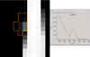 |
Fig. B.1. Single frame of the TESS target pixel file with the pipeline mask shown as a dashed red line. The so-called bleed trail of γ Leo contaminates the flux of AD Leo. The graph on the right shows the projection of the pixel column with the strongest contamination (shown as the green line in the TPF). We applied our own light-curve extraction using a customized mask (solid yellow line) and corrected the flux level of the second strongest contaminated pixel (see text). |
Appendix C: Parameters from the spectral analysis of XMM-Newton data
We provide the elemental abundances for the quiescent corona of AD Leo during the XMM-Newton observation derived from the RGS spectrum (Table C.1) and the evolution of the spectral parameters throughout the exponential flare phase obtained from the EPIC/pn spectra in time slices of roughly equal photon statistics (Table C.2) as explained in Sect. 2.1.1.
Coronal abundances derived from the quiescent RGS spectrum with respect to the solar photospheric abundances from Asplund et al. (2009) and first ionization potential.
Best-fit parameters of the time-resolved X-ray spectral analysis of the EPIC/pn data throughout the exponential phase of the flare.
Appendix D: Period search on the TESS light curve
Following our previous work that we cited in Sect. 2.2, we used three methods to search for the rotation period of AD Leo: We computed the generalized Lomb-Scargle periodogram (GLS; Zechmeister & Kürster 2009), we determined the autocorrelation function (ACF), and finally, we fit the light curve with a sine function. The GLS implementation we used1 can only process up to 10000 data points. Therefore, we had to bin the light curve by a factor of ten to a resolution of 200 s. The light curve was then phase-folded with the period found with each of the methods. The result of our period search is shown in Fig. D.1. Through visual inspection, we selected the best-fitting period. For the TESS Sector 45 light curve of AD Leo analyzed in this work, the GLS and the sine fitting resulted in periods that are consistent with each other and with values from the literature (see Sect. 2.2.1), while the ACF did not show an unambiguous periodic pattern and hence failed to identify the rotation period (see Fig. D.1). We thus adopted the average of the GLS and sine-fitting period, Prot = 2.194 ± 0.004. The error was calculated with the formulas given by Gilliland & Fisher (1985).
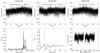 |
Fig. D.1. Results of the three period-search methods (GLS, ACF, and sine-fitting) for AD Leo observed in TESS Sector 45. The top panels show the light curve phase-folded with the periods obtained with the different methods. The bottom panel shows the GLS periodogram, the ACF, and the original detrended light curve with the sine fit. |
All Tables
Coronal abundances derived from the quiescent RGS spectrum with respect to the solar photospheric abundances from Asplund et al. (2009) and first ionization potential.
Best-fit parameters of the time-resolved X-ray spectral analysis of the EPIC/pn data throughout the exponential phase of the flare.
All Figures
|
Fig. 1. Light curves of the superflare. Top panel: XMM-Newton EPIC/pn count rate in 0.2 − 12 keV (red) and in the GOES band (1.5 − 12.4 keV; green). The binning adapted to the TESS light curve in FAST cadence (20 s) is shown in the bottom panel (black circles), where it is overlaid with the time derivative of the X-ray luminosity (open diamonds). The thick dashed vertical line marks the time of the peak of the flare flux in the TESS light curve, and the dash-dotted lines mark the boundaries of the intervals used for the time-resolved spectral analysis of the X-ray data. For a better display of the main flare phase, a cut has been set to the abscissa values such that the tail of the flare is not shown. |
| In the text | |
|
Fig. 2. Time evolution throughout the superflare for parameters derived from the XMM-Newton and TESS data. Upper panel: flaring plasma temperature and EM. Middle panel: flaring plasma abundances and electron density. The abundances of all elements are tied to the Fe abundance using the ratios determined for the quiescent state from the RGS spectrum that are listed in Table C.1. Lower panel: thermal energy in the flaring plasma, compared with the total radiated energy in the X-ray and optical bands. |
| In the text | |
|
Fig. 3. Time evolution of the mean temperature and EM associated with the flare. The red line represents a linear least-squares fit to this first phase of the flare decay (when the flaring emission is still much higher than the slightly variable background corona). The blue line is the fit to the whole exponential decay. |
| In the text | |
|
Fig. 4. Empirical relation of WLF energy and GOES flux for solar flares and power-law fits performed by Namekata et al. (2017) on them using a linear regression method and a linear regression bisector method (solid and dashed lines). The red line is our fit including the AD Leo superflare, which yields in the double logarithmic form (log EWLF = a + b ⋅ log FGOES), a slope b = 1.150 ± 0.005, and an axis-offset of a = 34.711 ± 0.007, where the uncertainties are the standard deviations of the fit. |
| In the text | |
|
Fig. B.1. Single frame of the TESS target pixel file with the pipeline mask shown as a dashed red line. The so-called bleed trail of γ Leo contaminates the flux of AD Leo. The graph on the right shows the projection of the pixel column with the strongest contamination (shown as the green line in the TPF). We applied our own light-curve extraction using a customized mask (solid yellow line) and corrected the flux level of the second strongest contaminated pixel (see text). |
| In the text | |
|
Fig. D.1. Results of the three period-search methods (GLS, ACF, and sine-fitting) for AD Leo observed in TESS Sector 45. The top panels show the light curve phase-folded with the periods obtained with the different methods. The bottom panel shows the GLS periodogram, the ACF, and the original detrended light curve with the sine fit. |
| In the text | |
Current usage metrics show cumulative count of Article Views (full-text article views including HTML views, PDF and ePub downloads, according to the available data) and Abstracts Views on Vision4Press platform.
Data correspond to usage on the plateform after 2015. The current usage metrics is available 48-96 hours after online publication and is updated daily on week days.
Initial download of the metrics may take a while.