| Issue |
A&A
Volume 667, November 2022
|
|
|---|---|---|
| Article Number | A116 | |
| Number of page(s) | 16 | |
| Section | Galactic structure, stellar clusters and populations | |
| DOI | https://doi.org/10.1051/0004-6361/202244070 | |
| Published online | 15 November 2022 | |
From ridges to manifolds: 3D characterization of the moving groups in the Milky Way disc
1
Departament de Física Quàntica i Astrofísica (FQA), Universitat de Barcelona (UB), C Martí i Franquès, 1, 08028 Barcelona, Spain
2
Institut de Ciències del Cosmos (ICCUB), Universitat de Barcelona (UB), C Martí i Franquès, 1, 08028 Barcelona, Spain
3
Institut d’Estudis Espacials de Catalunya (IEEC), C Gran Capità, 2-4, 08034 Barcelona, Spain
e-mail: This email address is being protected from spambots. You need JavaScript enabled to view it.
4
Université de Strasbourg, CNRS, Observatoire astronomique de Strasbourg, 11 rue de l’Université, 67000 Strasbourg, France
Received:
20
May
2022
Accepted:
25
July
2022
Abstract
Context. The details of the effect of the bar and spiral arms on the disc dynamics of the Milky Way are still unknown. The stellar velocity distribution in the solar neighbourhood displays kinematic substructures, which are possibly signatures of these processes and of previous accretion events. With the Gaia mission, more details of these signatures, such as ridges in the Vϕ − R plane and thin arches in the Vϕ − VR plane, have been revealed. The positions of these kinematic substructures, or moving groups, can be thought of as continuous manifolds in the 6D phase space, and the ridges and arches as specific projections of these manifolds.
Aims. Our aim is to detect and characterize the moving groups along the Milky Way disc, sampling the galactocentric radial and azimuthal velocities of the manifolds through the three dimensions of the disc: radial, azimuthal, and vertical.
Method. We developed and applied a novel methodology to perform a blind search for substructure in the Gaia EDR3 6D data, which consists in the execution of the wavelet transform in independent small volumes of the Milky Way disc, and the grouping of these local solutions into global structures with a method based on the breadth-first search algorithm from graph theory. We applied the same methodology to simulations of barred galaxies to validate the method and for comparison with the data.
Results. We reveal the skeleton of the velocity distribution, uncovering projections that were not possible before. We sample nine main moving groups along a large region of the disc in configuration space, covering up to 6 kpc, 60 deg, and 2 kpc in the radial, azimuthal, and vertical directions, respectively, extending significantly the range of previous analyses. In the radial direction we find that the groups deviate from the lines of constant angular momentum that one would naively expect from an epicyclic approximation analysis of the first-order effects of resonances. We reveal that the spatial evolution of the moving groups is complex and that the configuration of moving groups in the solar neighbourhood is not maintained along the disc. We also find that the azimuthal velocity of the moving groups that are mostly detected in the inner parts of the disc (Arcturus, Bobylev, and Hercules) is non-axisymmetric. For Hercules we measure an azimuthal gradient of −0.50 km s−1 deg−1 at R = 8 kpc. We detect a vertical asymmetry in the azimuthal velocity for the Coma Berenices moving group, which is not expected for structures originating from a resonance of the bar, supporting the previous hypothesis of the incomplete vertical phase mixing of the group. In our simulations we extract substructures corresponding to the outer Lindblad resonance and the 1:1 resonances and observe the same deviation from constant angular momentum lines and the non-axisymmetry of the azimuthal velocities of the moving groups in the inner part of the disc.
Conclusions. This data-driven characterization is a starting point for a holistic understanding of the moving groups. It also allows for a quantitative comparison with models, providing a key tool to comprehend the dynamics of the Milky Way.
Key words: Galaxy: disk / Galaxy: kinematics and dynamics / Galaxy: structure / Galaxy: evolution / methods: data analysis
© M. Bernet et al. 2022
 Open Access article, published by EDP Sciences, under the terms of the Creative Commons Attribution License (https://creativecommons.org/licenses/by/4.0), which permits unrestricted use, distribution, and reproduction in any medium, provided the original work is properly cited.
This article is published in open access under the Subscribe-to-Open model. This email address is being protected from spambots. You need JavaScript enabled to view it. to support open access publication.
1. Introduction
The stellar velocity distribution in the solar neighbourhood (SN) has long been a key element in our understanding of the structure of the Milky Way (MW) (Dehnen & Binney 1998; Skuljan et al. 1999; Famaey et al. 2005; Antoja et al. 2008). Historically, several overdensities in this velocity distribution have been identified and discussed (Pleiades, Hyades, Sirius). These moving groups, as they are usually called, can be related to the orbital resonances of the bar and spiral arms of the Galaxy (Kalnajs 1991; Dehnen 2000; Antoja et al. 2011; Fragkoudi et al. 2019; Monari et al. 2019a) and/or attributed to ongoing phase mixing related to external perturbations (Minchev et al. 2009; Gómez et al. 2012; Antoja et al. 2018; Ramos et al. 2018; Hunt et al. 2018a; Khanna et al. 2019; Laporte et al. 2019, 2020).
The latest releases of the Gaia mission (Gaia Collaboration 2018a, 2021a) have provided a full 6D phase-space catalogue of 7.2 million stars, increasing the size and precision of any previous survey by several orders of magnitude. This has been a game changer in many fields of astrophysics. In the SN the new high resolution velocity distribution has revealed a complex substructure with several thin arches never observed before (Gaia Collaboration 2018b). When extending the study to the entire disc, large ridges appeared in the R − Vϕ (respectively, galactocentric radius and azimuthal velocity) diagram covering several kiloparsecs (Antoja et al. 2018; Kawata et al. 2018; Fragkoudi et al. 2019).
Orbits in a barred potential can be trapped into resonances (Weinberg 1994). Dehnen (2000) showed that in a short–fast bar scenario (i.e. Ωb = 50 km s−1 kpc−1) the transition between two types of non-axisymmetric orbital families across the bar’s outer Lindblad resonance (OLR) can explain the bi-modality formed by Hercules and the rest of the velocity distribution in the SN if the Sun is placed just outside the OLR of the bar (ROLR ≈ 7.2 kpc). This scenario was consistent with the gas dynamics measurements of the inner MW at the time. Later on, studies of star counts and the kinematics of the inner MW suggested that the bar might be longer and slower than previously thought (Portail et al. 2017). In this case, the OLR would be placed further out (ROLR ≈ 10.5 kpc, perhaps matching other groups such as the Arch/Hat instead of Hercules) and co-rotation (CR) would be closer to the SN (RCR ≈ 6 kpc). Pérez-Villegas et al. (2017) and Monari et al. (2019a) then explained Hercules as the overdensity formed by the orbits trapped at the CR, librating around the Lagrangian points of a long–slow bar. This moving group created by CR seems to be less pronounced than the one produced by the OLR (Binney 2018; Hunt et al. 2018b). However, Hunt et al. (2018a) showed that the addition of spiral structure in combination with the CR might create a strong distinct Hercules, and Chiba et al. (2021) showed that a decelerating Galactic bar could enhance the occupation on resonances, being able to reproduce Hercules through the CR resonance. This shows that the value of the pattern speed (Ωb) of the MW bar and the exact link between substructures and resonances are still a matter of debate, and more observables are needed to obtain a final answer.
In this direction, Ramos et al. (2018, hereafter R18), used the wavelet transform (WT, Starck & Murtagh 2002; Chereul et al. 1999) to detect and characterize the kinematics of the moving groups along the disc. They matched the spatial evolution of the groups with the ridges in the R − Vϕ plane. They claimed that some of the arches follow lines of constant energy at a given volume, which could be related to phase mixing processes (Minchev et al. 2009; Gómez et al. 2012), and that others follow lines of common angular momentum in the radial direction, as expected approximately in the case of resonant kinematic substructures (e.g. Quillen et al. 2018a). They also claimed that the observed changes in the azimuthal direction for the Hercules moving group are consistent with being produced by the OLR of a short–fast bar (Dehnen 2000; Fux 2001; Antoja et al. 2014). The long–slow paradigm is relatively recent and there have been few analyses on the azimuthal variations of a substructure caused by CR. Monari et al. (2019b) found that the Hercules angular momentum changes significantly with azimuth as they predicted analytically for the co-rotation resonance of an old long–slow bar. They showed that the only way to obtain a similar change in azimuth for an OLR origin of Hercules would be if the orbits are still far from phase-mixed in the bar potential (bar perturbation younger than 2 Gyr; see also Trick et al. 2021).
The link between the moving groups across the neighbourhoods in R18 was made visually, using a scatter plot of two variables and colour as a third variable. Therefore, the analysis of the moving groups link was restricted to three variables. Since VR and Vϕ are compulsory to select the moving groups, this limitation restricted the analysis to one dimension in space (either radial or azimuthal). The vertical direction was not explored.
The correlation between the position of the moving groups (overdensities in VR − Vϕ) and the ridges (overdensities in R − Vϕ) indicate that both are projections of the same substructure in the 6D phase-space onto different planes. The positions of these kinematic substructures, also known as moving groups, can be described as continuous manifolds in 6D phase space, and the ridges and arches as specific projections of these manifolds. Our goal in this article is to extend the idea introduced in R18 by automatizing the n-dimensional link of the moving groups to avoid the limitation of projecting the data. Using this process, we intend to move from a ridge-moving group paradigm to a manifold paradigm, where we sample the position of these manifolds in the (R, ϕ, Z, VR, Vϕ) space for each moving group.
We present a novel methodology of detecting these manifolds in a dataset. It is based on the execution of the WT in independent small volumes, and the relation of these local solutions in global substructures with an algorithm based on the breadth-first search (BFS) algorithm from graph theory. With this methodology we processed the Gaia EDR3 6D data and detect the positions of the groups across the MW disc. We also sampled the manifolds of two test particle simulations with a fast (Ωb = 50 km s−1 kpc−1) and a slow (Ωb = 30 km s−1 kpc−1) bar, both to test our methodology and to compare it to the data.
The Gaia DR3 (Gaia Collaboration 2022a) catalogue includes a larger and updated sample of radial velocities (33 M of stars, Gaia Collaboration 2022b), which covers a larger region of the MW disc and increases the resolution (number of stars and precision) of Gaia EDR3. This provides finer observables to untangle the different contributions in the complex dynamics of the Galaxy. To exploit these data in their totality new strategies must be developed (e.g. Contardo et al. 2022), such as the one we present here, to avoid the current limitations of the analysis.
This paper is organized as follows. In Sect. 2 we describe the observational data we used. In Sect. 3 we introduce the methodology we developed. In Sect. 4 we show the results of the application of the method to Gaia EDR3 data. In Sect. 5 we present and analyse the simulations. In Sect. 6 we compare the results from the data and the simulations, and with previous results in the literature. Finally, in Sect. 7 we list the main conclusions of this work.
2. Data and sample preprocessing
The Gaia Early Data Release 3 (EDR3) consists of an updated and enlarged source list, with improved astrometry and photometry. About 7.2 million stars have proper motion and a radial velocity measurements in the Gaia DR2, most of which are transferred to EDR3 (Seabroke et al. 2021; Torra et al. 2021). For this section we use a subset of these stars with photo-geometric distances from Bailer-Jones et al. (2021), derived from a probabilistic approach including colour and apparent magnitude information.
Distance is a critical parameter in the computation of the motion and position of the star in the 6D study of the MW, and a major source of uncertainty. This is why, in order to improve the quality of the sample, we also apply a cut in relative parallax error:
 (1)
(1)
The resulting sample contains 6 059 648 sources.
In Appendix A, we study the errors that an overestimation or an underestimation of the distance could produce in our results. We determine that, in general, this error would be below 2 km s−1 for a distance bias of ±10%, and that it would not affect the overall trend of the groups.
We use a cylindrical galactocentric coordinate system, fixing the reference at the Galactic Centre with the radial direction (R) pointing outwards from it, the azimuthal (ϕ) negative in the direction of rotation, and the vertical component (Z) positive towards the north galactic pole. To transform Gaia observables to positions and velocities in this reference frame, we take the Sun to be at R⊙ = 8.178 kpc (GRAVITY Collaboration 2019), ϕ⊙ = 0° and Z⊙ = 0.0208 kpc (Bennett & Bovy 2019). For the solar motion, we use U⊙ = 11.1, vcirc + V⊙ = 248.5, W⊙ = 7.25 km s−1 (Schönrich et al. 2010; Reid & Brunthaler 2020).
3. Method
The data described in the previous section contains the 6D variables of position (R, ϕ, Z) and velocity (VR, Vϕ, VZ) of the stars. Inside small volumes, cuts in (R, ϕ, Z), the moving groups appear as well-defined overdensities in the velocity distribution VR − Vϕ (R18), which are easy to detect. However, we know that at large spatial scales the position of the overdensities in the velocity space changes (ridges in R − Vϕ). Therefore, if we use larger volumes to construct the velocity distribution, the overdensities will blur and become undetectable.
In this section we present the novel method that we developed to extract these large kinematic substructures from a dataset. It is divided into two steps: the execution of the WT in independent small volumes of the MW disc, and the relation of these local solutions in global substructures with an algorithm based on the BFS algorithm from graph theory (Moore 1959, described in Sect. 3.2).
3.1. Local wavelet transform
We partition the data in a dense grid of small volumes (hereafter pixels) in the spatial coordinates. We construct it as follows:
-
Radial direction (Ri): [5, 14] kpc in steps of 0.04 kpc,Rbin = ±0.24 kpc around each centre;
-
Azimuthal direction (ϕj): [ − 34, 34] deg in steps of 0.8 deg,ϕbin = ±2.4 deg around each centre;
-
Vertical direction (Zk): [ − 1, 1] kpc in steps of 0.08 kpc,Zbin = ±0.24 kpc around each centre.
This produces a dense grid of 2 700 000 pixels, with a maximum volume overlap between consecutive pixels of 83.3%. This bin size is bigger than that used in R18. When reaching regions far from the Sun, the statistical significance of the moving groups decreases and a bigger bin is the only way to obtain a robust determination of the group velocity. The drawback for this enlarged bin is that any inhomogeneity of the sample within a volume (e.g. due to the local extinction, the selection function, a change in the sampled populations) can bias the mean position of the stars, and therefore its kinematics. We tested this effect using a smaller bin, and we estimate the impact to be below 2 km s−1 for the bin size used.
For each pixel we construct the velocity distribution (VR, Vϕ) diagram of the stars in it as a 2D histogram with bins of 1 km s−1 (see background histogram in Fig. 1). R18 showed that the overdensities form thin arches elongated around large ranges of VR, with a small variation in Vϕ. The use of 2D peak detection algorithms (like the one in R18) is sub-optimal for arch-like structure detection. When analysing regions with few observations, the search for peaks is translated into a very noisy determination of VR, and uncontrollable correlations between VR and Vϕ (movement along the arch). To avoid this, we slice each VR − Vϕ diagram in vertical columns (bins in VR), and run a 1D WT in the Vϕ histogram of each column: radial velocity (VR): −100 – 100 km s−1 in steps of 10 km s−1, VR bin = ±15 km s−1 around each centre.
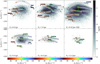 |
Fig. 1. Moving group detection in different neighbourhoods along the radial direction. For each moving group a parabolic fitting of the substructures associated with each group is included (highlighted in grey). Each moving group contains several structures, corresponding to different VR bins. The largest structure in each group is used as its representative (dots with larger black contours and the moving group name on top). There are two examples of bimodalities, which serve as evidence of the complex evolution of the arch morphology (Sirius at R = 8.16 kpc and Arch/Hat at R = 10.4 kpc). |
Since we are detecting each part of the arch separately, we avoid the movement along the arch of the overdensities, breaking the degeneracy between VR and Vϕ in the detection. To detect the peaks, we use the algorithm developed in Du et al. (2006) implemented in scipy (Virtanen et al. 2020) as find_peaks_cwt. This method performs the 1D WT in a range of length scales. A peak is then selected if it is present in enough scales consecutively. In our execution, we use a range of scales of [5, 10] km s−1, with steps of 1 km s−1. We keep the peak if it is present in more than two scales consecutively. With this configuration of scales, we lose the thin resolution that we could extract in regions with a large number of sources, but we gain robustness in the detection of the large structures in poorly sampled regions. Since the scope of this work is the large-scale behaviour of the groups, we consider this approach to be better.
At the end of the execution, the peak p inherits the spatial position from the pixel, VR from the position of the radial velocity bin, and Vϕ from the result of the WT detection. Therefore, a peak has the coordinates
 (2)
(2)
3.2. Breadth-first search resolution with online interpolator
We defined the pixels to have large overlaps; for example, two adjacent pixels will share 83.3% of their volume. Therefore, a given substructure in consecutive pixels will have an almost identical shape.
We consider a pair of peaks from consecutive pixels to be adjacent if they are in the same VR bin and if their distance in Vϕ is smaller than 4 km s−1. In R18, the maximum slope found in a moving group is 33 km s−1 kpc−1. In our grid the step is 0.04 kpc, which translates into a maximum change of ≈1 km s−1 between adjacent pixels. This 4 km s−1 limit in the adjacency is a compromise between including very steep groups (about 4 times that detected in R18) and reducing the number of adjacencies, which will determine the computational cost of the next step.
It sometimes occurs, especially in poorly sampled regions, that a peak from one pixel can be exactly in the middle of two peaks in the other pixel. In these cases we do not consider any of the peaks adjacent. With this consideration, two adjacent peaks are always strong candidates to belong to the same substructure.
This adjacency information constructs an enormous net of linked peaks. Ideally, substructures will be isolated subsets of peaks in this net. These are groups of peaks with no adjacencies to any peak outside their group.
In graph theory these nets of linked points are called graphs and the isolated groups are the connected components of a graph. A very common algorithm to extract these connected components is the BFS algorithm, which proceeds as follows:
-
Add (enqueue) the initial peak p to the queue1 Q;
-
Select (dequeue) the top peak ptop of the queue Q;
-
Visit all the peaks padj adjacent to ptop. For each adjacent peak, if we have already visited it, ignore the peak. If it is the first time we see the peak, enqueue it;
-
If there are still peaks in the queue, return to step 2;
-
If the queue is empty, our connected component is the list of visited peaks.
Given an initial peak p0, Algorithm 1 (see below) returns the entire substructure where it belongs. By repeating the process for all the non-matched peaks we can extract all the substructures.
1: queue Q
2: list V
3: add p0 to V and enqueue in Q
4: while Q not empty do
5: pit ← dequeue Q (remove and assign)
6: for all padj adjacent to pit do
7: if padj not in V then
8: add pad j to V, enqueue in Q
9: end if
10: end for
11: end while
12: return V
This solution would be enough in an ideal case, but in practice undersampling and Poisson noise especially in regions far from the Sun produce confusion and jumps between structures that a straightforward BFS implementation cannot filter out.
In order to avoid these jumps between structures, we include an extra step in the algorithm. While the BFS is running, the peaks already matched give us information about the structure. Therefore, in order to accept a new peak, we require it to be consistent with the current structure.
Let us suppose we have a group V of already-visited peaks (the current substructure we are extracting). To see if a peak p is consistent with this substructure we select all the peaks in V in a small subset S ⊂ V around p. With this local sample we can compute a linear fit
 (3)
(3)
of the subset S around p and predict the expected Vϕ of the substructure in a given position. This works under the assumption that the manifold that follows the substructure is derivable and we can compute its first-order approximation locally.
This prediction is already absorbing the offset in the structure position produced by its slope in a certain direction. Therefore, the criterion in the acceptance of a new peak should be stricter than that in the first adjacency step. Our limit in the resolution is the 1 km s−1 bin in the Vϕ histogram, and we include an extra tolerance of 0.5 km s−1. If the distance between the peak azimuthal velocity Vϕ, p (Eq. (2)) and the prediction is smaller than 1.5 km s−1, we consider the peak to be consistent with the structure. We encapsulate this in the is_consistent_with function (Algorithm 2). We provide a summary of the final algorithm in pseudocode (Algorithm 3).
1: S = V(|Rpadj – RV| < Rfit &
|ϕpad j – ϕV| < ϕfit &
|Zpadj| – ZV| < Zfit)
2: f (R, ϕ, Z) = Vϕ ← linear_fit(S|padj)
3: if |f((R, ϕ, Z)padj ) – Vϕ, padj < d then
4: return True
5: else
6: return False
7: end if
8: Rfit = 1 kpc, ϕf it = 4 deg, Zfit = 0.2 kpc, and d = 1.5 km s−1.
1: queue Q
2: list V
3: add p0 to V and enqueue in Q
4: while Q not empty do
5: pit ← dequeue Q (remove and assign)
6: for all padj adjacent to pit do
7: if padj not in V and is_consistent_with(padj, V) then
8: add padj to V, enqueue in Q
9: end if
10: end for
11: end while
12: return V
4. Results
Within the 3D grid the method extracted hundreds of structures, covering 2.5 to 6 kpc in R and 30 to 60 deg in ϕ. In R18 the arches in the SN and the radial direction were carefully characterized and matched to the groups previously studied in the literature. We rely on this matching to associate the results of our methodology with the different groups and arches.
We end up with a sample of 99 structures, each one associated with one of the nine main moving groups: Arcturus, Bobylev, Hercules, Horn, Hyades, Sirius, Coma Berenices, Arch/Hat (R18, and references therein), and AC (see Anti-Centre newridge 1 in Gaia Collaboration 2021b). Each structure traces the position of the moving group along the space at a given VR. Therefore, each group of structures traces the manifold of the position of the moving groups in the (R, ϕ, Z, VR, Vϕ) space. For each moving group we selected the largest structure as its representative. These representatives were used to study the behaviour of the groups in R − ϕ and R − Z projections, and are described in the following sections.
In Fig. 1 we show the selected groups in several neighbourhoods in the radial direction. In each arch we highlight its representative with a large black border. As explained in Sect. 3.1, our goal in this work is to be able to perform this analysis in a large extent of the disc, so we tuned the detection parameters to obtain a robust detection of the main structures in noisy regions (see R > 10 kpc in Fig. 1), and this required the use of larger spatial bins. Because of this, the thin arches observed in the Gaia velocity distribution in the SN are slightly washed out.
The methodology links the structures in a given VR, but does not provide the link of the arches in VR − Vϕ. The complex nature of the arches formed by the moving groups at different positions in the disc and the high level of noise result in a sub-optimal global link of the arches in the velocity distribution. Therefore, we only provide a tentative manual link of the structures, based on the study of R18. In the rest of the paper we use this arch link as a qualitative tool in the analysis, but the main conclusions are based on the properties of the individual parts of the arches, which are determined by the described methodology.
This linking procedure provides interesting results, different than in previous studies. For instance, the evident link of the Arch/Hat at R = 9.4 kpc creates an asymmetric arch shape for this structure at the SN. This could be an artefact of the detection of Arch/Hat at VR > 60 km s−1 or physical evidence of an unknown behaviour related to its origin. We note that tagging the groups in the SN and assuming that they remain united across the disc is a clear oversimplification. In the data we see that Sirius is formed by two arches at SN, but these arches merge into a single one at the outer parts of the disc (pannels R = 8.16, 9.4 kpc in Fig. 1). The same happens for Arch/Hat at R = 10.4 kpc. In the simulation (Sect. 5) we observe the same behaviour for the overdensities related to the OLR. So far, this simplification is useful for the discussion and comparison to the state of the art. Moreover, the lack of data far away from the SN does not allow a robust arch characterization. In future releases an automatized arch detection will be needed to disentangle the complex orbit distribution.
4.1. Radial direction
The first evidence of large-scale substructure in the dynamics of the disc was the presence of ridges in the R − Vϕ plane, directly related to the moving groups observed in the SN. Therefore, the first exercise we were able to do with the manifolds was to extract their subsets in the radial direction (i.e. ϕ = 0 deg, Z = 0 kpc) and plot them in R − Vϕ plane, coloured by VR (Fig. 2). In the top panel, we show the representative groups, tagged with their literature names. In the bottom panel, we show the rest of the structures as beams of lines that define the morphology of the corresponding moving groups. As expected, when tracing the different moving groups along R we observe diagonal lines in R − Vϕ, matching the already known ridges.
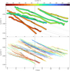 |
Fig. 2. Azimuthal velocity of the kinematic substructures in the radial direction, ϕ = 0°, Z = 0 kpc as a function of the radius and coloured by their radial velocity. Each dashed grey line corresponds to the best fit of a structure’s constant angular momentum line. Top: structures corresponding to the main peak of a moving group, tagged with the name from the literature. Bottom: secondary peaks of the moving groups. The usual way to observe this projection is using the number of stars or the mean VR in each bin (see Fig. 1 in Fragkoudi et al. 2019). The different lines delineate the skeleton of the distribution and its complexity. |
After comparison with R18, we detected the same moving groups, but we managed to extend their detection by several kiloparsecs. The results in the inner and outer part of the disc (R < 6.5 kpc and R > 10 kpc) are noisy due to Poisson noise. The Gaia DR3 release will improve the detection of groups in these regions, but even if we exclude this part the groups extend far beyond the range seen in other studies (see Fig. 6 in R18). This extension of the structures is due to a major improvement in the methodology and to the use of the updated astrometric Gaia EDR3 data. The lower error in proper motion and parallax increases the concentration of the moving groups in the undersampled regions.
In Fig. 2 we can see how the slope of the lines in radius is not constant across the different groups. In the top plot groups like Arcturus, Hercules, and Arch/Hat present slopes that are significantly steeper than Sirius and AC. However, this slope is not a common characteristic in all the parts of the arch of a group. For instance, in the bottom plot we can see that Arcturus is very steep at VR = 30 − 40 km s−1 (orange lines) and flattens for the negative part of the arch (VR = −20 km s−1, blue lines). We observe that secondary peaks have very different azimuthal and radial velocities when they start to show up at the inner radius, but end up having very similar azimuthal velocity at larger radii. This corresponds to a flattening of the arches in the velocity distribution as R increases. This is not observed in the simulations (Sect. 5), and could be an effect of the centroid of the distribution dominating in the case of undersampling in these regions.
As for the global shape of the lines, the resonant effects of the bar and spiral arms are expected to create kinematic substructures that, from an epicyclic approximation analysis of the first-order effects, have an almost constant vertical angular momentum LZ = RVϕ (Sellwood 2010; Quillen et al. 2018b). Thus, if the moving groups have a bar resonance origin, we might naively expect their azimuthal velocities to follow lines ∝R−1 (dashed grey lines in Fig. 2 top panel). In Ramos et al. (2018) (their Fig. 6), this trend is observed for Hercules and Hyades. When extending the analysis to a larger region, we find that the groups deviate from the lines of constant angular momentum. In Appendix B we compute the reduced chi-squared ( ) parameter for all the groups. The only group that is statistically well approximated globally by this Vϕ ∝ R−1 trend is Arch/Hat. We come back to this in Sect. 6.
The ridges are usually studied in R − Vϕ diagrams coloured by density or mean VR (see Fig. 1 in Fragkoudi et al. 2019). By doing these projections, the complexity of the moving groups (e.g. arch curvature, bi-modalities, arch disruption) is lost, offering only a partial understanding of the sample. With our methodology we can now visualize this complexity in a single plot. For instance, we can observe how the VR − Vϕ arch corresponding to the Arcturus moving group is a horizontal arch at R = 8 kpc (structures with different VR and common Vϕ), but that it curves towards the inner radius (the different structures fan out). This spreading clearly depends on the VR, which is a sign of a curved arch. Mixed with Arcturus, we are able to observe the morphology of Bobylev at VR > 50 km s−1. In the previously mentioned projections, the visualization of both structures is not possible since the mean VR blends the two contributions.
Beyond the detection and characterization of ridges in the radial direction, the main contribution of our method is the blind search of these kinematic structures in the three spatial dimensions at the same time. Next we focus on the representative of each moving group and study their kinematics in 3D space: the azimuth submanifold (Z = 0 kpc) in Sect. 4.2 and the vertical submanifold (ϕ = 0 deg) in Sect. 4.3.
4.2. Azimuth submanifold
We first do a cut in the structures around Z = 0 kpc (|Z|< 0.2 kpc) to observe the behaviour of the different moving groups as a function of R and ϕ. We obtain surfaces covering up to ±25 deg (≈3.5 kpc at solar radius). This is the first time that the moving groups are traced along the Z = 0 kpc plane with this completeness.
In Fig. 3, apart from the already studied decrease in Vϕ with R, we can see how the Arcturus, Bobylev, and Hercules moving groups present a slope in the azimuthal velocity along the azimuth, whereas the Horn, Sirius, and Arch/Hat moving groups present an axisymmetrical behaviour of the azimuthal velocity along the azimuth, as expected in an axisymmetric potential.
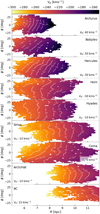 |
Fig. 3. Mean azimuthal velocity of the representative groups in the R − ϕ projection, for |Z|< 0.2 kpc. The contours of regions with the same velocity are shown for clarity (in white). The Arcturus, Bobylev, and Hercules moving groups present a constant slope in the variation of azimuthal velocity along azimuth, whereas the Horn, Sirius, and Arch/Hat moving groups present an axisymmetrical behaviour of the azimuthal velocity along azimuth. |
It is interesting to quantify the variation of Vϕ with ϕ for the structures. We evaluate this slope2 ∂Vϕ/∂ϕ at a given R by restricting the structure to this R value and doing a linear fitting of the surfaces in ϕ − Vϕ. We compute the slope in the radius that minimizes the error in the fitting. The resulting values are −0.40 km s−1 deg−1 at R = 7 kpc for Arcturus, −0.63 km s−1 deg−1 at R = 7 kpc for Bobylev, −0.50 km s−1 deg−1 at R = 8 kpc for Hercules, −0.04 km s−1 deg−1 at R = 10 kpc for Sirius, and −0.01 km s−1 deg−1 at R = 10 kpc for Arch/Hat.
In Monari et al. (2019b) they study the mean angular momentum evolution in ϕ for Hercules in an analytical model. In the case of a co-rotation origin, they predict that the angular momentum Jϕ of Hercules at the solar radius must significantly decrease with increasing azimuth. Their model predicts the slope to be around −8 km s−1 kpc deg−1, and they observe a similar trend in the Gaia DR2 data. Our equivalent value in angular momentum would be −4 km s−1 kpc deg−1, which is smaller than the predicted value.
In some parts of the disc the mean azimuthal velocity in the plane for the total 6D sample decreases with increasing azimuth at a constant radius (see Fig. 10 in Gaia Collaboration 2018b, R = 8 − 10 kpc). This is the behaviour that we observe for Arcturus, Bobylev, and Hercules. It would be worth investigating the relative contribution of each moving group to the total sample to understand the relation between these individual groups and the total average motion, but we will postpone this to a future study.
4.3. Vertical submanifold
We also studied the projection in the R − Z plane (|ϕ|< 10 deg, see Fig. 4). In all the structures but Coma Berenices (see below), we observe decreasing |Vϕ| values for increasing |Z|. In addition, Arcturus, Bobylev, and Hercules, the same structures that show steeper slope in azimuth, present a clear symmetry around Z = 0 kpc. Arch/Hat is also very symmetric in Z. Instead, Horn, Hyades, and Sirius present a steeper decrease in |Vϕ| for Z > 0 kpc with respect to the other moving groups, and a more constant value for Z < 0 kpc. Finally, AC does not have enough signal at this point to analyse it properly.
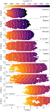 |
Fig. 4. Mean azimuthal velocity of the groups in the R − Z projection, for |ϕ|< 10 deg. The contours of regions with the same velocity are shown for clarity (in white). Coma Berenices clearly presents an increasing |Vϕ| with Z, and thus strong vertical asymmetry. We measure a constant vertical slope of ∂Vϕ/∂Z = −15 km s−1 kpc−1. The rest of the structures show vertical symmetry. |
Coma Berenices clearly presents an increasing |Vϕ| with Z, and thus strong vertical asymmetry. We note that outside the range of R = [7, 10] kpc, this moving group shows a change in behaviour in all the spatial projections (Figs. 2–4) possibly because our methodology is linking it to other close structures. Therefore, focusing only on the [7, 10] kpc range, we measure a constant vertical slope of ∂Vϕ/∂Z = −15 km s−1 kpc−1, clearly different to the other groups and to the predictions from models with vertical symmetry.
It would be interesting to obtain a measurement of the vertical curvature of the moving groups at each radius, as is done in the previous section with the slope in azimuth and with the vertical slope in Coma Berenices. With noisy data, each order of derivatives increases its uncertainty and the measurements we obtained were not significant enough. In the future, with better data and/or a robust analytical model to fit the curvature at all radii at the same time, this measurement could be produced.
5. Simulations
In this section we apply the same methodology to the simulations. This has two main goals: evaluating the performance of our method in a case where there are no selection effects, and allowing a comparison of the data to a model where a particular and known perturbation is present. In our case we used a series of test particle simulations with 60M particles. The initial conditions and the Galactic potential are described in Romero-Gómez et al. (2015). In particular, the disc has a local radial velocity dispersion of σVR = 30.3 km s−1 at the radius of 8.5 kpc. We integrated the initial conditions, first in the axisymemtric potential of Allen & Santillan (1991) for 10 Gyr; then we introduced the Galactic bar potential adiabatically during 4 bar rotations (2.46 Gyr for the slow bar and 1.47 Gyr for the fast bar), to finally integrate another 4 bar rotations. The Galactic bar consists of the superposition of two aligned Ferrers ellipsoids (Ferrers 1877), one modelling the triaxial bulge with semi-major axis of 3.13 kpc and the second modelling the long thin bar with semi-major axis of 4.5 kpc. We used two simulations, where the bar rotates as a rigid body with a constant pattern speed of 30 and 50 km s kpc−1. For the slow bar, the CR was located at 7.3 kpc and the OLR at 12.2 kpc. For the fast bar, the CR was located at 4.3 kpc and the OLR at 7.6 kpc. We used the final snapshot of the simulations, and assumed that the bar is 30 deg in azimuth with respect to the Sun in the direction of rotation, close to the estimations for the MW (Bland-Hawthorn & Gerhard 2016, references therein).
In these final snapshots we execute the methodology described in Sect. 3 and obtain an optimal detection of the moving groups in a large range of the sample. These robust results match the predictions from previous works, and validate the performance of our methodology in a known dataset. However, we found some substructures related to the centroid of the velocity distribution whose changes with azimuth, radius, and height are mostly related to the rotation curve of the model. In this section we only show the substructure related to bar resonances and ignore the rest of the groups extracted by the methodology.
The selected moving groups are shown in the VR − Vϕ projection in Fig. 5 (as done in Fig. 1 for the real data). In the simulation the moving groups also show arches in this projection, which we are able to detect at several radii. Again, we can show the groups projected in the radial direction (Fig. 6, compare Fig. 2). In Figs. 5 and 6, the top panels show the structures of the fast bar model (depicting the effects of the OLR and 1:1 resonance); the bottom panels show the structures of the slow bar model (only the effects of the OLR appear). In the following sections we analyse the fast bar model (Sect. 5.1) and the slow bar model (Sect. 5.2) in detail.
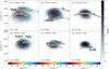 |
Fig. 5. Moving group detection in different neighbourhoods along the radial direction in the simulations (compare Fig. 1). Top row: fast bar model. Bottom row: slow bar model. |
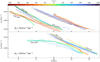 |
Fig. 6. Azimuthal velocity of the kinematic substructures in the radial direction (ϕ = 0°, Z = 0 kpc) for the test particle simulations as a function of the radius, and coloured by their radial velocity. We include dashed grey lines corresponding to constant angular momentum lines as a guide. Top: structures for the fast bar model. Bottom: structures for the slow bar model. The detections of the OLR (for both the fast and slow model) and the 1:1 (only detected for the fast case) are marked on top of the lines. Here the complex morphology of the arches appears in a single image. |
As explained in the introduction, a fast bar model places Hercules near the OLR of the bar. In this model Arch/Hat can be explained as the 1:1 resonance. Instead, the slow bar model places Hercules in the CR of the bar and Arch/Hat in the OLR. Therefore, in this paper we use the term ‘Hercules-like’ for structures in the simulation that can be related to Hercules in the data (i.e. generated by OLR for the fast bar model and by CR for the slow bar model), and ‘Arch/Hat-like’ for the structures that can be related to the Arch/Hat (i.e. induced by the 1:1 for the fast bar model and by the OLR for the slow bar model).
In Fig. 6 it is clear that the global position of the overdensities does not follow exactly the lines of constant angular momentum predicted for small epicyclic amplitudes (Vϕ ∝ R−1). In the radial direction the curvature of the OLR_bott structures is opposite in the two models. In addition, the fact that the structures merge at some radius is clear evidence that they follow a trend that is different from ∝R−1. The first-order prediction for resonances is suboptimal for Vϕ values far from the circular velocity. In Fig. 6 we observe how the radial slope of the structures differs more from the prediction at small and large Vϕ values.
5.1. Fast bar model
In the fast rotating bar simulation (Ωb = 50 km s−1 kpc−1) we are able to detect substructures related to the OLR and the 1:1 resonance with our methodology. As expected, both structures present an arch shape in the VR − Vϕ diagram (Fig. 5, top). The complete sampling and the simplicity of the simulation allows us to trace these arches unequivocally and observe their morphology in ranges up to 6 kpc in the radial and azimuthal directions, characterizing with strong robustness not only their position in the velocity space, but also the trend of the central and outer part of the arch separately. We note that the simulation has been integrated for 4 bar rotations, which places this model in the regime of a young fast bar, as defined in Monari et al. (2019b).
In the top part of Fig. 6, the bi-modality of the OLR and the 1:1 resonance are clearly observed. For the OLR, at R < 7 kpc we observe a Hercules-like arch (OLR_bott), extending to a maximum VR of 40 km s−1 (orange line at top). In this same region we also observe a symmetric arch at the top of the distribution labelled OLR_top, with a maximum in VR = 0 km s−1 (green line at top). At R between 7 and 8 kpc, the VR-negative part of the bottom arch (VR around −10 km s−1) continues to decrease in |Vϕ|, and the positive part of the arch (VR > 20 km s−1) merges with the top arch (OLT_top) to form a unique structure covering the whole radial velocity range. This unique arch, labelled OLR_comm, has its maximum at VR = −40 km s−1 (blue line at top). The arch configurations at R = 7, 9, and 11 kpc can also be seen in the top row of Fig. 5.
The signature of the 1:1 resonance (Arch/Hat-like structure) is less prominent than in the case of the OLR. In Fig. 5 (top row, R = 11 kpc) we observe a bi-modality in the histogram, with the upper part of the distribution being more prominent at negative VR values and the lower part more prominent in the positive VR range. In the R − Vϕ diagram (Fig. 6, top panel) we see that at the inner radius we mostly detect negative VR, and at the outer parts mostly positive VR, giving more evidence of this bi-modality. Due to the small prominence of the resonance, we are not able to detect it when it is located in the centre of the distribution.
As we did with the real data, we exploit the 3D extent of the structures and show their trends in the azimuth submanifold. In Fig. 7 we show the R − ϕ projection of the azimuthal velocity for different parts of the arches (compare Fig. 3). The black lines in these panels show the azimuthal slope of Vϕ in each radius (right vertical axes).
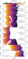 |
Fig. 7. Fast bar model. Mean azimuthal velocity of a selection of groups in the R − ϕ projection, for |Z|< 0.5 kpc. The contours of regions with the same velocity are shown for clarity (in white). The slope of the linear fitting (ϕ, Vϕ) is shown (in black) for every R column, in units of [km s−1 deg−1]. The 3σ error of the slope is shown in a translucent region around the line. |
The OLR_comm structures present a discontinuity around R = 8 kpc. In Fig. 6 this can be seen as the sudden drop in Vϕ in the green-turquoise lines at R ∼ 8 kpc (VR = −20, −10, 0 km s−1). A similar discontinuity is present in two panels of the OLR_bott structure in Fig. 7. The peak detection algorithm guarantees a minimum distance between peaks for robustness. Therefore, when two arches merge, the algorithm stops detecting one of them a short time before the merge. Even so, a few spurious detections can act as a bridge for the algorithm and and make it join the two structures. Since the arches are merging, the algorithm described in Sect. 3.2 (Algorithm 3) detects a continuity and the structures are detected together.
It is important to remember that Fig. 7 shows a young fast bar, which is known to introduce azimuth correlations, especially around the OLR (see Fig. A1 in Trick et al. 2021). For most of the structures, we see an azimuth slope of Vϕ that depends on radius. Interestingly, some structures have negative ∂Vϕ/∂ϕ, such as Hercules in the real data, and others have a positive slope. We observe three main structures with different patterns:
-
Rows 1–4, and 7. Upper part of the OLR bimodality. Before crossing the rotation curve (R ≈ 8 kpc), the ∂Vϕ/∂ϕ slope of the structure is constant along all the VR values. For R > 8 kpc, a correlation appears between ∂Vϕ/∂ϕ and VR. This is a sign that the OLR_comm arch shown in Fig. 5 (top row, R = 9 kpc) is moving to negative VR values in the VR − Vϕ diagram as ϕ increases (when VR is more positive, its |Vϕ| decreases faster with ϕ).
-
Rows 5–7 (R < 8 kpc). Hercules-like part of the distribution. The slope in azimuth decreases as R increases. The contour lines merge when approaching the bar’s long axis (ϕb = −30 deg).
-
Rows 8 and 9. Arch/Hat-like part of the distribution. The slope in azimuth is constant along the different detected parts of the arch, and tends to flatten for increasing R values.
5.2. Slow bar model
In the slow rotating bar simulation (Ωb = 30 km s−1 kpc−1), we are able to detect the Arch/Hat-like overdensity caused by the OLR along a wide range of radius values, covering up to 6 kpc (Figs. 5 and 6, bottom panels). In the radial direction we observe three different structures related with the OLR. Two of them have negative VR and the other has positive VR. The negative VR structures (OLR_top and OLR_bott) present a clear bi-modality in Vϕ. In the VR − Vϕ diagram (Fig. 5, bottom), the OLR_top forms a flat arch and the OLR_bott forms a curved arch. In the positive VR regime (orange-red lines), we observe one single structure (OLR_comm) compatible with OLR_top at R = 10 to 11 kpc, which continues to decrease its azimuthal velocity with R in a constant slope and merges OLR_bott from R = 12 kpc to the outer parts of the disc.
Again, we can exploit the 3D extension of the manifolds to study how these groups are evolving in the R − ϕ projection. In Fig. 8 (as in Fig. 7, but for the slow bar model) we observe two main structures, corresponding to the different parts of the OLR bi-modality (whose upper part corresponds now to the Arch/Hat-like group). Rows 1–3 are the top part of the OLR bi-modality. It presents a constant slope in azimuth (∂Vϕ/∂ϕ = −0.1 km s−1 deg−1 at R = 12 kpc), flattening as R increases, similar to the Arch/Hat-like part observed in Fig. 7 for the fast bar. Rows 4–7 show the bottom part of the bi-modality. The slope is less constant, and we observe the same decrease in R as in the Hercules-like part of the fast bar model.
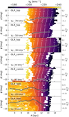 |
Fig. 8. Slow bar model. Mean azimuthal velocity of a selection of groups in the R − ϕ projection, for |Z|< 0.5 kpc (compare Fig. 7). In this simulation the shape of the arches is maintained along ϕ (same slope for all VR values), with a constant displacement to bigger |Vϕ| as ϕ increases. |
We do not detect overdensities caused by CR. In general, the expected Hercules-like moving group caused by CR is less prominent than when formed by the OLR (Binney 2018; Hunt et al. 2018b), especially if higher order modes are missing from the bar model. In addition, if the velocity dispersion of the disc is too large in this region, we could have less trapping and less resolution. Another explanation could be that the length of the bar in our models does not favour CR trapping. In the future, we aim to perform the same analysis with other models to analyse this effect (e.g. Sormani et al. 2022).
In Fig. D.1 we show the Vϕ − R projection coloured by mean VR. In this figure we observe a very faint red overdensity in the CR region, but much weaker compared to the rest of the detected resonances in the fast and the slow bar models.
6. Discussion
Simulations that contain only a bar perturber offer us the possibility to characterize its effects in a robust way. With this characterization, we can then compare the manifolds extracted from the simulation with those seen in the data. As explained in the introduction, one of our goals with the characterization of the manifolds is to search for kinematic observables that distinguish resonances from short/fast or long/slow bars.
Radial direction. First, we focus on the slope, shape, and evolution of the moving groups in the data and the simulation along the radial direction (Figs. 2 and 6).
The global gradient of the structures in the radial direction deviates from the first-order prediction for resonances (curves following Vϕ ∝ R−1) in the data and the simulations, as expected in more realistic cases, even if they have a resonance origin. In the simulations we see that the lines are less curved than the simple prediction and some parts of the OLR_bott have even the opposite curvature. This is also observed in the data, where all the moving groups are less steep in the inner parts of the disc than the prediction, and Hercules and Arcturus present the same opposite curvature pattern as the OLR_bott.
We see in the Vϕ − R projection coloured by mean VR of the slow bar scenario of our simulations (Fig. D.1) that the co-rotation overdensity is not significant enough. This is discussed in the Introduction and in the previous section, and could be related to the specificities of the model considered here. In the fast bar scenario a Hercules-like structure is formed at R = [6, 8] kpc, which shows an arch shape with a maximum in VR = 40 km s−1 (Fig. 5, top left panel), consistent with the Hercules moving group in the data. In this same radial region the top part of the OLR forms an arch in negative VR, which can be related to Horn. Finally, from R = 8 kpc towards the outer parts of the disc, the OLR forms a single arch with a maximum in VR = −20 km s−1. A similar arch, present at all the radial velocities, was already observed in the models by Bovy (2010). In the data this region (R > 9 kpc, Vϕ < −170 km s−1) contains very few stars, and we did not detect any group there.
The other feature commonly associated with bar resonances is the Arch/Hat moving group. For a fast bar, it can be explained by the 1:1 resonance trapping region, and for a slow bar it matches the position of the OLR. In the data, the number of stars with R > 10 kpc is low. Therefore, the quality of the shape characterization of the Arch/Hat moving group is poor. Even so, in the panel R = 10.4 kpc in Fig. 1 our method finds a tentative arch split around VR = 10 km s−1. This would match the split we detect between the OLR_comm and OLR_top structures in the slow bar model (Fig. 6, bottom panel at R = 11 kpc). In the fast bar simulation, the prominence of the 1:1 resonance is low and we can only detect it in regions far from the centroid of the distribution. Even with this limited detection, we do not observe a bi-modality in the negative VR region, which would be a way to discriminate between resonances.
Azimuth submanifold. In both simulation models, for the Arch/Hat-like moving groups we observe a constant positive slope of |Vϕ| in azimuth which tends to flatten (get closer to 0 km s−1 deg−1) as R increases. In these Arch/Hat-like groups, the slope of the azimuthal velocity in azimuth does not depend on VR (Figs. 7 and 8). In the data (Fig. 3), the Arch/Hat group is very noisy. Therefore, as discussed in the previous paragraph it is still complicated to use the Arch/Hat velocities for a final relation to a specific resonance.
In Fig. 7 we can observe the different parts of the OLR resonance in the fast bar. The Hercules-like overdensity (R = [6, 8] kpc) shows a constant positive slope of |Vϕ| in azimuth common along all VR. In opposition, the trapping region of the resonance OLR_comm has a slope that depends on the VR. This can be interpreted as the arch moving along VR in the VR-Vϕ diagram when moving in azimuth, which is observed at the OLR in other simulations of a young bar far from phase-mixed (Dehnen 2000; Bovy 2010; Trick et al. 2021). Since we have the complete information of the moving groups in the data, we can reproduce the same analysis of the moving group slope at different VR for some moving groups in the data. In Figs. C.1 and C.2, we show this slope for Hercules and Hyades, respectively. We do not observe this dependence in VR for any of the groups. In the velocity distribution this can be observed as the moving group arches increasing their |Vϕ| along the azimuth, but no displacement along VR.
Vertical submanifold. For the resonces of the bar, the vertical displacement of Vϕ should be dominated to first order by the vertical potential of the Galaxy (Al Kazwini et al. 2022). In our results the vertical curvature of all the moving groups (except for Coma Berenices) at a common radius is very similar, thus matching the analytical prediction. This means that this data is a good candidate to constrain the 3D structure of the potential. To second order, we could try to distinguish different curvatures of different resonances. In Al Kazwini et al. (2022) the displacement of the resonances at Z = 1 kpc with respect to the galactic plane is measured to be 8 km s−1 kpc−1 for the corotation, 6 km s−1 kpc−1 for the OLR, and 4 km s−1 kpc−1 for the 1:1 resonance. Our maximum resolution, given by the Vϕ histogram at each pixel, is 1 km s−1 kpc−1. Therefore, disentangling which resonances create each moving group with the vertical information is beyond our current capabilities.
In the vertical behaviour of the moving groups, a clear outlier is Coma Berenices. In Quillen et al. (2018b) (also Monari et al. 2018; Laporte et al. 2019), the Coma Berenices moving group is observed to be present only at negative galactic latitudes, showing evidence of incomplete vertical phase mixing. With the new EDR3 data and our methodology, we are able to detect the group in a larger extension and at positive and negative galactic latitudes, but it does show a clear vertical asymmetry in its azimuthal velocity. We measure a constant vertical slope of ∂Vϕ/∂Z = −15 km s−1 kpc−1. In the plots of a phase spiral coloured by Vϕ (Antoja et al. 2018), it is seen that there must be a correlation between Z and Vϕ (higher |Vϕ| values at positive Z). This slope in Coma Berenices could be a projection of this correlation.
7. Conclusions
We have sampled, with the Gaia EDR3 6D data, the manifolds tracing the main moving groups in the SN along the (R, ϕ, Z, VR, Vϕ) space, in an automatic way. We have revealed the skeleton of the velocity distribution in a multidimensional space that we can then explore along the radial direction, and characterize in the azimuth and vertical submanifolds. This methodology was successfully tested with two simulations of the effects of a dynamically young bar. We were able to observe and quantify the spatial evolution of the observed moving groups in a large range of about 3 kpc around the sun. Our main results and conclusions are the following:
-
The azimuthal velocity of the moving groups in the radial direction does not follow lines of constant angular momentum, deviating from our naive first-order prediction for resonances. In the simulations, resonant structures also deviate from this simple prediction, demanding more complex analytic predictions.
-
The spatial evolution of the moving groups is complex. The moving group configuration observed in the SN is not maintained throughout the disc. The relative position between the arches and their curvature changes across space, and the different moving groups split and merge several times. This is expected in a context of bifurcating orbital families, for example in the case of resonances.
-
In our slow bar simulation we observe a bi-modality created by the OLR in the outer parts of the disc. This bi-modality is also observed in the Arch/Hat moving group in the data. This intriguing agreement could favour the slow bar scenario, and opens the possibility of a test with future data.
-
The Arcturus, Bobylev, and Hercules moving groups present a positive slope of their Vϕ location with the azimuth. We measure this slope to be −0.50 km s−1 deg−1 at R = 8 kpc for Hercules.
-
The azimuthal velocity of the Horn, Sirius and Arch/Hat moving groups presents an axisymmetrical behaviour. In both our simulations we observed a small azimuthal gradient in Vϕ in the Arch/Hat-like structures, although it approches 0 as R increases. This could be related to the young bar model we are using.
-
The vertical curvature of the moving groups is similar at the same R. These curvatures are dominated by the gravitational potential to first order, independently of the observed resonance. However, we find that the Coma Berenices group deviates from this behaviour, which points to a different dynamical origin that deserves further investigation.
-
In the fast bar simulation a correlation between ∂Vϕ/∂ϕ and VR is observed for the OLR trapping region. The region where this correlation is observed in the simulation (R > 9 kpc, Vϕ < −170 km s−1) is poorly sampled in Gaia EDR3, but this could potentially be used to give information on the pattern speed of the bar with better data.
Spiral arms, resonances with the bar, accretion events, and possibly other effects can contribute to the present phase space distribution from which we obtain our observables. Disentangling all the contributions of these dynamical processes is difficult. In this work we have shown the complexity of the phase-space structure that even a single mechanism (namely the bar) can produce. Our methodology allows a quantitative and robust measurement of the observed phase space substructure to be extracted, which can be then compared and/or fit to different models.
In this paper we have developed the methodology for the study of the disc with the Gaia data, and its formulation is easily generalizable. The same approach can be exported to other substructures in astrophysics (e.g. blind search for streams and shells in the halo) and even to datasets outside this field.
In the following months Gaia DR3 will revolutionize once again our field of research. The new 6D sample contains about 33M stars, covering a significantly larger region of the disc. During the review process, this new data was already being used in Lucchini et al. (2022) to reveal four new moving groups candidates in the SN. With this work, we are ready to process the Gaia DR3 data and extract its full potential.
A queue is a data structure similar to an array with limited access to the positions. One end is always used to insert data (enqueue) and the other is used to remove data (dequeue). Queue follows a first-in-first-out methodology, such that the data item stored first will be accessed first.
In our reference system a negative ∂Vϕ/∂ϕ slope corresponds to an increase in |Vϕ| with ϕ (a moving group with negative ∂Vϕ/∂ϕ moves upwards in the velocity distribution with ϕ).
Acknowledgments
We thank the anonymous referee for her/his helpful comments. This work has made use of data from the European Space Agency (ESA) mission Gaia (https://www.cosmos.esa.int/gaia), processed by the Gaia Data Processing and Analysis Consortium (DPAC, https://www.cosmos.esa.int/web/gaia/dpac/consortium). Funding for the DPAC has been provided by national institutions, in particular the institutions participating in the Gaia Multilateral Agreement. This work was (partially) funded by the Spanish MICIN/AEI/10.13039/501100011033 and by “ERDF A way of making Europe” by the “European Union” through grant RTI2018-095076-B-C21, and the Institute of Cosmos Sciences University of Barcelona (ICCUB, Unidad de Excelencia ‘María de Maeztu’) through grant CEX2019-000918-M. MB acknowledges funding from the University of Barcelona’s official doctoral program for the development of a R+D+i project under the PREDOCS-UB grant. TA acknowledges the grant RYC2018-025968-I funded by MCIN/AEI/10.13039/501100011033 and by “ESF Investing in your future”. BF, GM and PR acknowledge funding from the “Agence Nationale de la Recherche” (ANR project ANR-18-CE31-0006 and ANR-19-CE31- 0017) and from the European Research Council (ERC) under the European Union’s Horizon 2020 research and innovation programme (grant agreement No. 834148).
References
- Al Kazwini, H., Agobert, Q., Siebert, A., et al. 2022, A&A, 658, A50 [NASA ADS] [CrossRef] [EDP Sciences] [Google Scholar]
- Allen, C., & Santillan, A. 1991, Rev. Mex. Astron. Astrofis., 22, 255 [NASA ADS] [Google Scholar]
- Anders, F., Khalatyan, A., Queiroz, A. B. A., et al. 2022, A&A, 658, A91 [NASA ADS] [CrossRef] [EDP Sciences] [Google Scholar]
- Antoja, T., Figueras, F., Fernández, D., & Torra, J. 2008, A&A, 490, 135 [NASA ADS] [CrossRef] [EDP Sciences] [Google Scholar]
- Antoja, T., Figueras, F., Romero-Gómez, M., et al. 2011, MNRAS, 418, 1423 [NASA ADS] [CrossRef] [Google Scholar]
- Antoja, T., Helmi, A., Dehnen, W., et al. 2014, A&A, 563, A60 [NASA ADS] [CrossRef] [EDP Sciences] [Google Scholar]
- Antoja, T., Helmi, A., Romero-Gómez, M., et al. 2018, Nature, 561, 360 [Google Scholar]
- Bailer-Jones, C. A. L., Rybizki, J., Fouesneau, M., Demleitner, M., & Andrae, R. 2021, AJ, 161, 147 [Google Scholar]
- Bennett, M., & Bovy, J. 2019, MNRAS, 482, 1417 [NASA ADS] [CrossRef] [Google Scholar]
- Binney, J. 2018, MNRAS, 474, 2706 [NASA ADS] [Google Scholar]
- Bland-Hawthorn, J., & Gerhard, O. 2016, ARA&A, 54, 529 [Google Scholar]
- Bovy, J. 2010, ApJ, 725, 1676 [NASA ADS] [CrossRef] [Google Scholar]
- Chereul, E., Crézé, M., & Bienaymé, O. 1999, A&AS, 135, 5 [NASA ADS] [CrossRef] [EDP Sciences] [Google Scholar]
- Chiba, R., Friske, J. K. S., & Schönrich, R. 2021, MNRAS, 500, 4710 [Google Scholar]
- Contardo, G., Hogg, D. W., Hunt, J. A. S., Peek, J. E. G., & Chen, Y.-C. 2022, AJ, submitted [arXiv:2201.10674] [Google Scholar]
- Dehnen, W. 2000, AJ, 119, 800 [NASA ADS] [CrossRef] [Google Scholar]
- Dehnen, W., & Binney, J. J. 1998, MNRAS, 298, 387 [NASA ADS] [CrossRef] [Google Scholar]
- Du, P., Kibbe, W. A., & Lin, S. M. 2006, Bioinformatics, 22, 2059 [CrossRef] [Google Scholar]
- Famaey, B., Jorissen, A., Luri, X., et al. 2005, A&A, 430, 165 [CrossRef] [EDP Sciences] [Google Scholar]
- Ferrers, N. 1877, QJ Pure Appl. Math., 14, 1 [Google Scholar]
- Fragkoudi, F., Katz, D., Trick, W., et al. 2019, MNRAS, 488, 3324 [NASA ADS] [Google Scholar]
- Fux, R. 2001, A&A, 373, 511 [NASA ADS] [CrossRef] [EDP Sciences] [Google Scholar]
- Gaia Collaboration (Brown, A. G. A., et al.) 2018a, A&A, 616, A1 [NASA ADS] [CrossRef] [EDP Sciences] [Google Scholar]
- Gaia Collaboration (Katz, D., et al.) 2018b, A&A, 616, A11 [NASA ADS] [CrossRef] [EDP Sciences] [Google Scholar]
- Gaia Collaboration (Brown, A. G. A., et al.) 2021a, A&A, 649, A1 [NASA ADS] [CrossRef] [EDP Sciences] [Google Scholar]
- Gaia Collaboration (Antoja, T., et al.) 2021b, A&A, 649, A8 [EDP Sciences] [Google Scholar]
- Gaia Collaboration (Vallenari, A., et al.) 2022a, A&A, accepted [Google Scholar]
- Gaia Collaboration (Drimmel, R., et al.) 2022b, A&A, accepted [Google Scholar]
- Gómez, F. A., Minchev, I., Villalobos, Á., O’Shea, B. W., & Williams, M. E. K. 2012, MNRAS, 419, 2163 [CrossRef] [Google Scholar]
- GRAVITY Collaboration (Abuter, R., et al.) 2019, A&A, 625, L10 [NASA ADS] [CrossRef] [EDP Sciences] [Google Scholar]
- Hunt, J. A. S., Hong, J., Bovy, J., Kawata, D., & Grand, R. J. J. 2018a, MNRAS, 481, 3794 [NASA ADS] [CrossRef] [Google Scholar]
- Hunt, J. A. S., Bovy, J., Pérez-Villegas, A., et al. 2018b, MNRAS, 474, 95 [NASA ADS] [CrossRef] [Google Scholar]
- Kalnajs, A. J. 1991, Dynamics of Disc Galaxies, ed. B. Sundelius, 323 [Google Scholar]
- Kawata, D., Baba, J., Ciucǎ, I., et al. 2018, MNRAS, 479, L108 [Google Scholar]
- Khanna, S., Sharma, S., Tepper-Garcia, T., et al. 2019, MNRAS, 489, 4962 [Google Scholar]
- Laporte, C. F. P., Minchev, I., Johnston, K. V., & Gómez, F. A. 2019, MNRAS, 485, 3134 [Google Scholar]
- Laporte, C. F. P., Famaey, B., Monari, G., et al. 2020, A&A, 643, L3 [EDP Sciences] [Google Scholar]
- Lucchini, S., Pellett, E., D’Onghia, E., & Aguerri, J. A. L. 2022, Moving Groups Across Galactocentric Radius with Gaia DR3 [Google Scholar]
- Minchev, I., Quillen, A. C., Williams, M., et al. 2009, MNRAS, 396, L56 [NASA ADS] [CrossRef] [Google Scholar]
- Monari, G., Famaey, B., Minchev, I., et al. 2018, Res. Notes Am. Astron. Soc., 2, 32 [Google Scholar]
- Monari, G., Famaey, B., Siebert, A., Wegg, C., & Gerhard, O. 2019a, A&A, 626, A41 [NASA ADS] [CrossRef] [EDP Sciences] [Google Scholar]
- Monari, G., Famaey, B., Siebert, A., et al. 2019b, A&A, 632, A107 [NASA ADS] [CrossRef] [EDP Sciences] [Google Scholar]
- Moore, E. F. 1959, Proc. Int. Symp. Switching Theor., 1959, 285 [Google Scholar]
- Pérez-Villegas, A., Portail, M., Wegg, C., & Gerhard, O. 2017, ApJ, 840, L2 [Google Scholar]
- Portail, M., Gerhard, O., Wegg, C., & Ness, M. 2017, MNRAS, 465, 1621 [NASA ADS] [CrossRef] [Google Scholar]
- Quillen, A. C., Carrillo, I., Anders, F., et al. 2018a, MNRAS, 480, 3132 [NASA ADS] [CrossRef] [Google Scholar]
- Quillen, A. C., De Silva, G., Sharma, S., et al. 2018b, MNRAS, 478, 228 [NASA ADS] [CrossRef] [Google Scholar]
- Ramos, P., Antoja, T., & Figueras, F. 2018, A&A, 619, A72 [NASA ADS] [CrossRef] [EDP Sciences] [Google Scholar]
- Reid, M. J., & Brunthaler, A. 2020, ApJ, 892, 39 [Google Scholar]
- Romero-Gómez, M., Figueras, F., Antoja, T., Abedi, H., & Aguilar, L. 2015, MNRAS, 447, 218 [CrossRef] [Google Scholar]
- Schönrich, R., Binney, J., & Dehnen, W. 2010, MNRAS, 403, 1829 [NASA ADS] [CrossRef] [Google Scholar]
- Seabroke, G. M., Fabricius, C., Teyssier, D., et al. 2021, A&A, 653, A160 [NASA ADS] [CrossRef] [EDP Sciences] [Google Scholar]
- Sellwood, J. A. 2010, MNRAS, 409, 145 [NASA ADS] [CrossRef] [Google Scholar]
- Skuljan, J., Hearnshaw, J. B., & Cottrell, P. L. 1999, MNRAS, 308, 731 [NASA ADS] [CrossRef] [Google Scholar]
- Sormani, M. C., Gerhard, O., Portail, M., Vasiliev, E., & Clarke, J. 2022, MNRAS, 514, L1 [NASA ADS] [CrossRef] [Google Scholar]
- Starck, J.-L., & Murtagh, F. 2002, Astronomical Image and Data Analysis (Berlin Heidelberg: Springer), 291 [Google Scholar]
- Torra, F., Castañeda, J., Fabricius, C., et al. 2021, A&A, 649, A10 [NASA ADS] [CrossRef] [EDP Sciences] [Google Scholar]
- Trick, W. H., Fragkoudi, F., Hunt, J. A. S., Mackereth, J. T., & White, S. D. M. 2021, MNRAS, 500, 2645 [Google Scholar]
- Virtanen, P., Gommers, R., Oliphant, T. E., et al. 2020, Nat. Methods, 17, 261 [Google Scholar]
- Weinberg, M. D. 1994, ApJ, 420, 597 [NASA ADS] [CrossRef] [Google Scholar]
Appendix A: Distance Bias
We should be more worried about systematic errors in distance than about random errors since random errors would in principle only blur the structures. Systematic errors in distance may arise from the conversion from parallax to distance and the use of priors in the Bayesian procedures, for example. While it is difficult to evaluate the systematics in the distances that we used, one can perform some simple tests. In order to estimate the impact of a systematic error in the distance estimation we regenerated the sample using two worst-case scenarios: an overestimation of all distances by +10% and an underestimation by −10%. When comparing distances from StarHorse (Anders et al. 2022) and the photogeometric distances from Bailer-Jones et al. (2021), we see that for 80% of the stars the distance differences are smaller than 4% at 2 kpc and smaller than 7% at 3 kpc. The error that we consider in this test is thus larger than this difference.
In Fig. A.1 we show the results of the peak detection part of our methodology in the radial, azimuthal, and vertical directions for the three samples (original, −10% bias, and +10% bias). In the figure we observe that introducing this bias produces a contraction or expansion of some dimensions of the phase-space, thus slightly modifying the position of the moving groups.
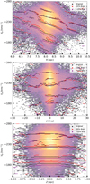 |
Fig. A.1. Peak detection of the methodology for the original, −10% bias, and +10% bias samples, in the radial, azimuthal, and vertical directions. |
Quantifying the difference in the position of the peaks, we can estimate the error that this bias could introduce. In general, the bias is more significant if the azimutal velocity of the group is far from the solar azimuthal velocity. For ridges in the |Vϕ|< |Vϕ, ⊙| region, an underestimate of the distance increases the |Vϕ| of the ridge, and a overestimate decreases the ridge |Vϕ|. For Hercules, this produces a bias of 3 km s−1 in the SN (Vϕ = −200 km s−1), for Arcturus the bias increases to 8 km s−1. The opposite effect is seen for stars in the |Vϕ|> |Vϕ, ⊙| region. For Arch/Hat, this bias is 5 km s−1 at R = 9 kpc (Vϕ = −280 km s−1). It is important to note that we only detect kinematic structures at these low and high azimuthal velocities close to the Sun, precisely in the region where a bias in the distance measurement is less likely, mitigating the possibility of a distance bias.
In the radial direction, both R and Vϕ are proportional to the distance. Therefore, when computing the slope ∂Vϕ/∂R the dependence on distance cancels out. This is why the slopes that we observe for the structures in the plane R-Vϕ (ridges) are maintained when the bias in the distance is introduced. In the azimuthal direction, an underestimation or overestimation of the distance produces a small negative or positive curvature of 2 km s−1 at |ϕ|=20 deg. In the vertical direction, an underestimate or overestimate of the distance produces a small positive or negative curvature of 2 km s−1 at Z = ±0.7 kpc.
Appendix B: Epicyclic approximation discrepancy
Here we test whether the structures in the radial direction (ridges) follow lines of constant angular momentum. To do this we use a reduced chi-squared ( ) test, considering a constant error in the detection of σ = 5 km s−1, which is half of the largest scale used in the wavelet. We compute the Lz which provides the best Vϕ = Lz/R fitting for each group (i.e. it minimizes the
  parameter). The best fitting curves are shown in Fig. 2. In Table B.1, we show the
  parameter for each group. With this parameter we can now compare the goodness of fit for each structure. There are three groups of results. In the first group the Arch/Hat is clearly well fitted by a line of constant angular momentum. A second group, formed by Arcturus, Bobylev, and AC, presents low chi-squared values, but is clearly incompatible with an optimal fitting. Finally, the shape of the rest of the structures is absolutely different from the lines of constant angular momentum.
Reduced chi-squared ( ) parameter for each group, from lowest to highest.
Appendix C: Azimuth submanifold along a group
In Figure 3 we show the azimuth submanifold of a representative for each group. In this appendix we extend this analysis and show how each part of the Hercules and Hyades arches is evolving. In addition, since we have already shown these plots, we include the extra information on the slope of Vϕ in azimuth at each radius. With this information, we can compare these groups to the resonances studied in the simulations (Figs. 7 and 8).
The Hercules moving group (Fig. C.1) presents a stable and constant slope of Vϕ in azimuth at the centre of the sample (R = [6.5, 8] kpc). In the limits of the sample, where the significance of the group is smaller compared to the sample, this slope tends to flatten for the regions with VR ≈ 0 and to become more steep in the large VR parts of the arch.
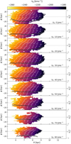 |
Fig. C.1. Mean azimuthal velocity of the groups in Hercules in the R − ϕ projection, for |Z|< 0.2 kpc. The contours of regions with the same velocity are shown for clarity (in white). The slope of the linear fitting (ϕ, Vϕ) is shown (in black) for every R column, in units of [km s−1 deg−1]. The 3σ error of the slope is shown in a translucent region around the line. The group has the same slope at all VR. This corresponds to a vertical displacement of the moving group in the VR-Vϕ diagram. |
The Hyades moving group (Fig. C.2) also presents a stable behaviour at all VR. In the negative VR end of the arch (top two rows in the figure) the group has a very low significance, thus leading to a noisy detection.
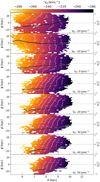 |
Fig. C.2. As in Fig. C.1, but for the mean azimuthal velocity of the groups in Hyades in the R − ϕ projection, for |Z|< 0.2 kpc. |
Appendix D: Extra projections of the simulations
This is the first time that a simulation has been studied using the projection shown in Fig. 6. In general, these studies are done in projections of ⟨VR⟩. In order to compare both results, in Fig. D.1 we show this projection for the simulation.
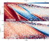 |
Fig. D.1. Mean radial velocity of the kinematic substructures in the radial direction (ϕ = 0°, Z = 0 kpc) for the test particle simulations as a function of the radius and the azimuthal velocity. Top: Fast bar simulation. Bottom: Slow bar simulation. |
In the top panel of Fig. D.1, in red, we see the Hercules-like overdensity, which steeply decreases in Vϕ around R = 8 kpc. The upper part of the OLR bi-modality continues to decrease in a less steep trend, with negative ⟨VR⟩ values above and positive values below the resonance. Finally, in the outer part of the disc we observe the effect of the 1:1 resonance, which shows a swap in ⟨VR⟩ sign when crossing the rotation curve.
In the bottom panel of Fig. D.1, CR should appear at R = 7.3 kpc, but we cannot see any significant structure in this region. In the outer parts of the disc we do observe the OLR placed at 12.2 kpc.
All Tables
All Figures
|
Fig. 1. Moving group detection in different neighbourhoods along the radial direction. For each moving group a parabolic fitting of the substructures associated with each group is included (highlighted in grey). Each moving group contains several structures, corresponding to different VR bins. The largest structure in each group is used as its representative (dots with larger black contours and the moving group name on top). There are two examples of bimodalities, which serve as evidence of the complex evolution of the arch morphology (Sirius at R = 8.16 kpc and Arch/Hat at R = 10.4 kpc). |
| In the text | |
|
Fig. 2. Azimuthal velocity of the kinematic substructures in the radial direction, ϕ = 0°, Z = 0 kpc as a function of the radius and coloured by their radial velocity. Each dashed grey line corresponds to the best fit of a structure’s constant angular momentum line. Top: structures corresponding to the main peak of a moving group, tagged with the name from the literature. Bottom: secondary peaks of the moving groups. The usual way to observe this projection is using the number of stars or the mean VR in each bin (see Fig. 1 in Fragkoudi et al. 2019). The different lines delineate the skeleton of the distribution and its complexity. |
| In the text | |
|
Fig. 3. Mean azimuthal velocity of the representative groups in the R − ϕ projection, for |Z|< 0.2 kpc. The contours of regions with the same velocity are shown for clarity (in white). The Arcturus, Bobylev, and Hercules moving groups present a constant slope in the variation of azimuthal velocity along azimuth, whereas the Horn, Sirius, and Arch/Hat moving groups present an axisymmetrical behaviour of the azimuthal velocity along azimuth. |
| In the text | |
|
Fig. 4. Mean azimuthal velocity of the groups in the R − Z projection, for |ϕ|< 10 deg. The contours of regions with the same velocity are shown for clarity (in white). Coma Berenices clearly presents an increasing |Vϕ| with Z, and thus strong vertical asymmetry. We measure a constant vertical slope of ∂Vϕ/∂Z = −15 km s−1 kpc−1. The rest of the structures show vertical symmetry. |
| In the text | |
|
Fig. 5. Moving group detection in different neighbourhoods along the radial direction in the simulations (compare Fig. 1). Top row: fast bar model. Bottom row: slow bar model. |
| In the text | |
|
Fig. 6. Azimuthal velocity of the kinematic substructures in the radial direction (ϕ = 0°, Z = 0 kpc) for the test particle simulations as a function of the radius, and coloured by their radial velocity. We include dashed grey lines corresponding to constant angular momentum lines as a guide. Top: structures for the fast bar model. Bottom: structures for the slow bar model. The detections of the OLR (for both the fast and slow model) and the 1:1 (only detected for the fast case) are marked on top of the lines. Here the complex morphology of the arches appears in a single image. |
| In the text | |
|
Fig. 7. Fast bar model. Mean azimuthal velocity of a selection of groups in the R − ϕ projection, for |Z|< 0.5 kpc. The contours of regions with the same velocity are shown for clarity (in white). The slope of the linear fitting (ϕ, Vϕ) is shown (in black) for every R column, in units of [km s−1 deg−1]. The 3σ error of the slope is shown in a translucent region around the line. |
| In the text | |
|
Fig. 8. Slow bar model. Mean azimuthal velocity of a selection of groups in the R − ϕ projection, for |Z|< 0.5 kpc (compare Fig. 7). In this simulation the shape of the arches is maintained along ϕ (same slope for all VR values), with a constant displacement to bigger |Vϕ| as ϕ increases. |
| In the text | |
|
Fig. A.1. Peak detection of the methodology for the original, −10% bias, and +10% bias samples, in the radial, azimuthal, and vertical directions. |
| In the text | |
|
Fig. C.1. Mean azimuthal velocity of the groups in Hercules in the R − ϕ projection, for |Z|< 0.2 kpc. The contours of regions with the same velocity are shown for clarity (in white). The slope of the linear fitting (ϕ, Vϕ) is shown (in black) for every R column, in units of [km s−1 deg−1]. The 3σ error of the slope is shown in a translucent region around the line. The group has the same slope at all VR. This corresponds to a vertical displacement of the moving group in the VR-Vϕ diagram. |
| In the text | |
|
Fig. C.2. As in Fig. C.1, but for the mean azimuthal velocity of the groups in Hyades in the R − ϕ projection, for |Z|< 0.2 kpc. |
| In the text | |
|
Fig. D.1. Mean radial velocity of the kinematic substructures in the radial direction (ϕ = 0°, Z = 0 kpc) for the test particle simulations as a function of the radius and the azimuthal velocity. Top: Fast bar simulation. Bottom: Slow bar simulation. |
| In the text | |
Current usage metrics show cumulative count of Article Views (full-text article views including HTML views, PDF and ePub downloads, according to the available data) and Abstracts Views on Vision4Press platform.
Data correspond to usage on the plateform after 2015. The current usage metrics is available 48-96 hours after online publication and is updated daily on week days.
Initial download of the metrics may take a while.