| Issue |
A&A
Volume 667, November 2022
|
|
|---|---|---|
| Article Number | A15 | |
| Number of page(s) | 24 | |
| Section | Planets and planetary systems | |
| DOI | https://doi.org/10.1051/0004-6361/202243436 | |
| Published online | 01 November 2022 | |
Impact of stellar flares on the chemical composition and transmission spectra of gaseous exoplanets orbiting M dwarfs
Institute of Astronomy,
KU Leuven, Celestijnenlaan 200D,
3001
Leuven, Belgium
e-mail: This email address is being protected from spambots. You need JavaScript enabled to view it.
Received:
28
February
2022
Accepted:
2
August
2022
Abstract
Context. Stellar flares of active M dwarfs can affect the atmospheric composition of close-orbiting gas giants, and can result in time-dependent transmission spectra.
Aims. We aim to examine the impact of a variety of flares, differing in energy, duration, and occurrence frequency, on the composition and transmission spectra of close-orbiting, tidally locked gaseous planets with climates dominated by equatorial superrotation.
Methods. We used a series of pseudo-2D photo- and thermochemical kinetics models, which take advection by the equatorial jet stream into account, to simulate the neutral molecular composition of a gaseous planet (Teff = 800 K) that orbits a M dwarf during artificially constructed flare events. We then computed transmission spectra for the evening and morning limb.
Results. We find that the upper regions (i.e. below 10 μbar) of the dayside and evening limb are heavily depleted in CH4 and NH3 up to several days after a flare event with a total radiative energy of 2 × 1033 erg. Molar fractions of C2H2 and HCN are enhanced up to a factor three on the nightside and morning limb after day-to-nightside advection of photodissociated CH4 and NH3. Methane depletion reduces transit depths by 100–300 parts per million (ppm) on the evening limb and C2H2 production increases the 14 μm feature up to 350 ppm on the morning limb. We find that repeated flaring drives the atmosphere to a composition that differs from its pre-flare distribution and that this translates to a permanent modification of the transmission spectrum.
Conclusions. We show that single high-energy flares can affect the atmospheres of close-orbiting gas giants up to several days after the flare event, during which their transmission spectra are altered by several hundred ppm. Repeated flaring has important implications for future retrieval analyses of exoplanets around active stars, as the atmospheric composition and resulting spectral signatures substantially differ from models that do not include flaring.
Key words: astrochemistry / planets and satellites: atmospheres / planets and satellites: composition / stars: flare
© T. Konings et al. 2022
 Open Access article, published by EDP Sciences, under the terms of the Creative Commons Attribution License (https://creativecommons.org/licenses/by/4.0), which permits unrestricted use, distribution, and reproduction in any medium, provided the original work is properly cited.
This article is published in open access under the Subscribe-to-Open model. This email address is being protected from spambots. You need JavaScript enabled to view it. to support open access publication.
1 Introduction
In the search for new exoplanets, M dwarfs are ideal targets due to their high abundance in the Galaxy (Bochanski et al. 2010). However, M-type stars are prone to high levels of stellar activity (Walkowicz et al. 2011; Loyd et al. 2016, 2018b) that can impact the radial velocity and/or transit signal of such systems through phenomena such as flaring (Tofflemire et al. 2012), star spots, plages and faculae (Boisse et al. 2011; Llama & Shkolnik 2015; Cauley et al. 2018; Roettenbacher et al. 2022; Bruno et al. 2022), and other activity-induced variability (Dumusque 2018; Rackham et al. 2019; Bellotti et al. 2022; Collier Cameron et al. 2021). Aside from the observational implications, the planet’s physical and chemical state can be altered by stellar activity as well due to, for example, coronal mass ejections (CMEs) and stellar particle events (SPEs) (Yamashiki et al. 2019; Atri 2017, 2020; Segura et al. 2010), winds (Vidotto et al. 2015; Vidotto & Cleary 2020; Chebly et al. 2022; Colombo et al. 2022), and stellar flares (Segura et al. 2010; Venot et al. 2016; Chadney et al. 2017; Tilley et al. 2019; Chen et al. 2021; Louca et al. 2022), the latter being sudden releases of radiative energy triggered by magnetic reconnection (Benz & Güdel 2010). Stellar flares result in a temporary increase in incident flux on the planet’s atmosphere, which in turn increases the photochemical reaction rates that can change the chemical composition. Photochemistry, and photolysis in particular, is a key driver of chemical disequilibrium in the atmospheres of close-orbiting, gaseous planets. Photolysis does not only deplete the upper layers from species such as CH4 and NH3, but it can enrich the middle regions with haze precursors such as HCN and C2H2 as well, particularly on cooler planets (Moses et al. 2011; Venot et al. 2012; Zahnle & Marley 2014; Agúndez et al. 2014; Moses 2014; Miguel & Kaltenegger 2014; Rimmer & Helling 2016; Drummond et al. 2016; Hobbs et al. 2019; Shulyak et al. 2020; Barth et al. 2021; Baeyens et al. 2022). Stellar flares thus have the potential to alter the chemical composition and, subsequently, alter the atmosphere’s signature in transmission spectra.
Several studies have been conducted that have used photo-and thermochemical kinetics models to study the effect of flares on exoplanetary atmospheres. Segura et al. (2010) tracked the water and ozone abundances of an Earth-like planetary atmosphere during a flare and SPE of its hypothetical M-type host star to address the consequences on the planet’s habitability. The authors constructed a time series from observations of the great flare event (GFE) of AD Leo, observed by Hawley & Pettersen (1991) on April 12, 1985. They found a strong depletion of water vapour at high altitudes and fluctuation in the ozone column depth of less than 1%, and thus concluded that a flare is insufficient to be a biological hazard. An accompanying proton event poses more danger as nitrogen oxides are formed at the cost of ozone, leaving the planetary surface unshielded from incident UV radiation. Tilley et al. (2019) performed a follow-up study considering repeated flaring. They found that multiple SPEs can reduce the initial ozone column depth of an Earth-like planet to 6% of its initial value in 10 yr time, while strictly radiative flaring overall has a limited impact. More recently, Chen et al. (2021) performed extensive three-dimensional coupled chemistry-climate model (CCM) simulations for rocky planets orbiting flaring G-, K-, and M-type stars. They found that recurring flares of K and M dwarfs drive the atmospheric composition into new equilibria that deviate from the pre-flare values (e.g. for various nitrogen and hydrogen oxides, ozone, and water vapour), but they find overall variations to the transmission spectra of less than 10 parts per million (ppm).
The impact of stellar flares has also been examined for H/He-dominated atmospheres of gas giants. Venot et al. (2016) studied the consequences of AD Leo’s GFE for a sub-Neptune (Teff = 1303 K) and super-Earth (Teff = 412 K). They found that prominent species in the atmosphere (such as H2O, OH, CO2, NH2, NO, and NH3) are affected. During the flare event, the transit depths of the super-Earth vary with less than 15 ppm, while the sub-Neptune experiences variations up to 150 ppm, situated in the CO/CO2 bumps at 4.6 and 14 μm. More interestingly, their post-flare compositions converge to a new steady-state after 1012 seconds (~30 000 yr) which results in transmission spectra that are different from their pre-flare state by up to 40 ppm and 500 ppm for the super-Earth and sub-Neptune, respectively. Additionally, Venot et al. (2016) explored the possibility of a repeated flaring every 5 h and found that this leads to variations up to 1200 ppm after only one day of such periodic flaring. Finally, taking into account the frequency of the flare’s occurrence as a function of its radiative energy could lead to accumulative changes in the chemical composition for both H2− and N2-dominated atmospheres, although the transmission spectra remain relatively unaffected (<12 ppm) (Louca et al. 2022).
Excluding Chen et al. (2021), the above studies are performed with one-dimensional photo- and thermochemical kinetics codes, thus ignoring longitudinal and latitudinal chemical exchange due to climate dynamics. Close-orbiting, tidally locked exoplanets are expected to host superrotating equatorial jet streams that reach velocities of several kilometres per second (Showman & Guillot 2002; Showman & Polvani 2011). Additional evidence for such a jet stream is inferred from many hot Jupiter phase curves where the brightest spot is shifted eastwards with respect to the substellar point (Knutson et al. 2007; Komacek et al. 2017; Zhang et al. 2018). When efficient enough, atmospheric dynamics can induce horizontal spatial variation in the distribution of chemical constituents (Cooper & Showman 2006; Mendonça et al. 2018; Drummond et al. 2020) and aerosols (Parmentier et al. 2013; Komacek et al. 2019; Steinrueck et al. 2019; Christie et al. 2021), which cannot be captured by one-dimensional codes. Subsequently, spatial asymmetries in the chemical and physical state of the atmosphere can give rise to differences between the morning and evening limb transmission spectra. For example, the evening limb is typically hotter (and thus more vertically extended) and resembles more the day-side composition, owing to eastwards transport from the dayside, while the morning limb is colder and polluted with nightside constituents (Baeyens et al. 2021). Taking into account these effects has been demonstrated to impact the final transmission spectrum (Caldas et al. 2019). Although flares only affect the dayside, vigorous circulation can redistribute chemical species throughout the atmosphere. Subsequently, this can affect the terminator regions which are probed with transmission spectroscopy. Therefore, we need to consider a multi-dimensional treatment when studying the atmosphere’s response to a flare event.
Stellar flares are known to span a wide range in energy, duration, emission line profile, occurrence frequency, peak flux, time evolution, etc. (Schaefer et al. 2000; Walkowicz et al. 2011; Davenport et al. 2012; Loyd et al. 2016, 2018a,b; Davenport 2016; Van Doorsselaere et al. 2017; Jackman et al. 2021a,b; Howard & MacGregor 2022). The GFE of AD Leo, used by Segura et al. (2010), Venot et al. (2016) and Tilley et al. (2019), is considered a superflare, with a total radiative output of ~1034 erg. These flares are thought to be rare, while lower-energy flares tend to occur much more frequently. As part of the MUSCLES Treasury Survey, Loyd et al. (2018a) used data of several M dwarfs to create an idealised flare model that has been used to study the effects of both rare high-energy and common low-energy flares on exoplanets (Chen et al. 2021; Louca et al. 2022).
In this paper, we aim to address how stellar flares of a M dwarf impact the neutral chemical composition of a close-orbiting, tidally locked gaseous planet (Teff = 800 K) with a superrotation-dominated circulation pattern. We explore a variety of stellar flares that differ in energy, duration and occurrence frequency. Additionally, we also investigate how the fluctuating composition alters the spectral signature of the planet in transmission. In Sect. 2, we discuss the general modelling strategy, including the chemical kinetics model with initial and boundary conditions and radiative transfer. Section 3 explains in more detail how the stellar flares are constructed. In Sect. 4, we present our results for different stellar flares and planets. We end with a discussion in Sect. 5, before concluding in Sect. 6.
2 Modelling tools
2.1 Pseudo-2D neutral disequilibrium chemistry
We use and slightly adapt the pseudo-2D chemical kinetics model of Agúndez et al. (2014) that takes into account photo- and thermochemistry, vertical mixing (by means of eddy diffusion) and horizontal transport induced by equatorial superrotation. In the model, the three-dimensional circulation pattern of the planet is approximated by a uniform zonal wind, described by a characteristic wind speed uwind, that advects chemical species eastwards around the equator. In practise, this is realised by a one-dimensional, rotating column that integrates the coupled continuity-transport equations for every species over a fixed longitude- and pressure-dependent thermal structure and pressure-dependent eddy diffusion profile. After an integration time of
 (1)
(1)
with wind period
 (2)
(2)
where nl is the number of longitudes and Rpl the planet radius, the column longitudinally shifts eastwards and again integrates the equations with updated initial conditions (advected chemical constituents, temperature structure and incident irradiation angle) specific for that longitude. Because the longitudinal spatial dimension is effectively time-dependent, this formalism is dubbed pseudo-2D. Although this model oversimplifies the complex three-dimensional dynamical structure of tidally locked exoplanets, it allows for relative computationally inexpensive use of chemical kinetics in a two-dimensional context. After several column rotations, the longitude- and pressure-dependent chemical composition converges to a periodic steady-state in which the molar fractions are constant with respect to longitude. We note that the wind period Pwind not only regulates the time it takes to complete one full column rotation but is in fact the same mathematical expression as τzonal, the zonal advection time-scale (e.g. Drummond et al. 2020), with a constant value for the otherwise pressure-dependent zonal wind speed u. However, τzonal should be considered an order-of-magnitude estimate for the zonal advection while Pwind is an exact quantity associated with the pseudo-2D chemistry model.
Several studies have used a pseudo-2D formalism to investigate the two-dimensional, periodic steady-state molecular distributions of exoplanet atmospheres (Agúndez et al. 2014; Venot et al. 2020b; Baeyens et al. 2021, 2022). However, in order to incorporate stellar flares into this framework, a time-dependent incident flux must be taken into account, and hence it is not guaranteed that a periodic steady-state will be reached. Instead, the chemistry model can be used to assess the dynamical response of the atmosphere to a perturbation of the incident radiation flux. Therefore, we have adjusted the initial implementation of Agúndez et al. (2014) such that the stellar flux can vary between column integrations. However, we note that all boundary conditions, including the stellar flux, remain fixed for the duration of one column integration (tcol).
By using the pseudo-2D chemistry code in a time-dependent manner, the time-longitude dependence puts a substantial constraint on the time sampling ∆t. Each longitude is only integrated every Pwind (= ∆t), which typically amounts to several days for Jovian-sized planets (e.g. Eq. (2) with uwind ~ km s−1). Such poor time sampling would heavily restrict us in probing the atmosphere’s response during and after a flare event. Therefore, we combine several pseudo-2D models and construct a fully two-dimensional, time-dependent atmosphere with higher time sampling. Our approach is illustrated in Fig. 1. The longitude which is integrated first (t = 0) in the pseudo-2D simulation was implemented by Agúndez et al. (2014) to coincide with the substellar point but in fact can be any arbitrary longitude. By starting the simulation on a different longitude, the time-longitude dependence ensures that we obtain information of different longitudes at the same time-steps as before. Therefore, we can run  pseudo-2D models with the same initial and boundary conditions but apply an offset to the starting longitude. By combining the information of all
  models on every time-step, we obtain a full two-dimensional time evolution of the atmosphere rather than the evolution of a single longitude as is the case for a single pseudo-2D model. Furthermore, the time-sampling of the combined atmosphere model, containing
  individual models, now becomes
  , which significantly improves the ability to study flare events on timescales shorter than several days. We note that the approach of combining separate models is justified because the very premise of the pseudo-2D formalism is that the chemical composition on longitude li at time ti can be computed from information of only li−1 at ti−1 and is thus independent from longitude li−1 at ti.
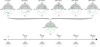 |
Fig. 1 Schematic diagram that illustrates how individual pseudo-2D chemistry models are combined into a single two-dimensional distribution. First, six |


2.2 Chemical network
To compute the production and loss rates in every integration, we have used the chemical network of Venot et al. (2020a) that involves 108 molecular species consisting of C, H, N, and O, linked by 1906 neutral-neutral reactions. Venot et al. (2020a) is an updated version of the network presented in Venot et al. (2012), which originated from the field of combustion chemistry and has been validated for temperatures and pressures relevant for hot Jupiters. The network is accompanied by 52 temperature-independent photoabsorption cross-sections (Venot et al. 2012; Hébrard et al. 2013; Dobrijevic et al. 2014). For further details regarding the chemical network such as lists of included molecules, reactions, and sources of the experimental data, we refer to Venot et al. (2012, 2020a).
2.3 Pre-flare thermal and chemical state
Baeyens et al. (2022; B22 hereafter) have computed climate and pseudo-2D photochemistry models for a grid of tidally locked gaseous exoplanets that covers a range of effective temperatures (Teff ∈ [400, 600,…, 2600 K]), surface gravities (g ∈ [l02, 103, 104] cm s−2), and spectral types of host stars (M5, K5, G5, F5). From their study, we use the two-dimensional thermal profile, pressure-dependent eddy diffusion coefficients Kzz, and zonal mean wind speed uwind of the model that corresponds to a Teff = 800 K, g = 103 cm s−2 planet orbiting a M5-type star. The temperature profile (lower panel, Fig. 2) was extracted from a three-dimensional general circulation model output between 200 and 10−4 bar. B22 considered an equatorial band between latitudes −20° < ϕ < 20°, from which they extracted a latitudinally weighted average that represents the equatorial thermal structure. From 10−4 bar down to 10−8 bar, the atmosphere is assumed isothermal with respect to pressure and adopts the temperature value of the layer with 10−4 bar. We refer to B22 for a discussion on the limitations of this isothermal extension.
We adopt the same pressure-dependent eddy diffusion coefficients (Kzz) as in B22 (upper panel, Fig. 2). The profile between 200 and 10−4 bar is computed by using the prescription of Komacek et al. (2019) (for more details, see Baeyens et al. 2021). For the upper layers (10−4 to 10−8 bar), B22 adopt a constant value of Kzz at 10−4 bar. The strength of the equatorial superrotating jet stream, that is the zonal mean wind speed uwind, is computed to be 1.529 km s−1 from the zonally averaged wind speeds by averaging between −20° < ϕ < 20° and 10 bar > p > 0.1 mbar.
For the pre-flare, periodic steady-state atmospheric composition, we repeat B22’s pseudo-2D simulation with a vertical resolution of 60 and an increased longitudinal resolution (nl = 180). We note that the elemental gas mixture is of solar metallicity and solar carbon-to-oxygen ratio (C/O = 0.55). We fix the orbital, stellar, and planetary parameters to the values used by B22. This encompasses the orbital separation of 0.01185 AU, planet mass Mpl = 0.74 Mpl, stellar radius R⋆ = 0.269 R⊙, and planet radius Rpl = 1.35 RJup. Together with uwind, the latter value leads to a wind period of Pwind 3.99 × 10⁵ s ≃ 4.6 days (Eq. (2)).
In order to construct the fully two-dimensional atmosphere model, we run  individual pseudo-2D models with each a longitudinal resolution of 180 (nl) for about one month (~2.4 × 10⁶ s) after the flare event and combine them following the method explained in Sect. 2.1 (see also Fig. 1). This implies that the actual integration time of a column (tcol) in an individual pseudo-2D model is twice as high as the time-sampling of the combined two-dimensional distribution
  . We note that the step of combining individual models is done in post-processing and does not affect the simulations themselves. We choose
  to strike a balance between the computational expense of
  runs and a sufficiently high longitudinal resolution (nl) of individual models. Furthermore,
  has to have a common denominator with nl in order to successfully apply the combing strategy explained in Sect. 2.1 as otherwise, the various pseudo-2D models would probe different longitudes at the fixed time-steps and cannot be combined to a full two-dimensional atmosphere model.
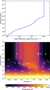 |
Fig. 2 Temperature and vertical mixing information of the Teff = 800 K planet that orbits a M5-type star considered in this work. Data generated by Baeyens et al. (2021). Upper: eddy diffusion coefficients Kzz with a constant value below 0.1 mbar. Lower: equatorial temperature structure with an isothermal upper atmosphere below 0.1 mbar. 0° denotes the substellar point. For pressure above 10 bar, the temperature increases with pressure to values above 1000 K so we have cut off the colourbar scale. |
2.4 Synthetic transmission spectra
We computed synthetic transmission spectra during and after the flare event between 0.5 μιm and 30 μm by using petitRADTRANS (Mollière et al. 2019) in low resolution mode (λ/∆λ = 1000). We include line absorption opacities of C2H2, CO2, CO, OH, HCN, NH3, CH4, H2O, and H2, Rayleigh scattering opacity of H2 and He, and continuum opacity from collision induced absorption by H2−H2 and H2−He. Because atomic species other than hydrogen, carbon, nitrogen, and oxygen do not participate in the chemical disequilibrium modelling, we do not include species such as sodium and potassium in the radiative transfer calculations, despite their observed presence in gaseous exo-planet atmospheres (e.g. Redfield et al. 2008; Charbonneau et al. 2002; Nikolov et al. 2015; Chen et al. 2018). We also omit aerosol opacity sources in the radiative transfer computations to isolate effects of the flare on the chemical composition.
We use petitRADTRANS to acquire one-dimensional transmission spectra of the evening and morning limb separately. This means that we extract a column from the longitude-temperature profile (Fig. 2) and chemical distribution at the relevant longitude, from which we compute the transit depths. We adopt a reference pressure of 0.01 bar for a planet radius Rpl (= 1.35 RJup), from which the transit depths are computed. We note that the adopted pseudo-2D formalism only represents the equatorial regions (−20° < ϕ < 20°) while the entire terminator contributes to the transmission spectrum. Our calculated spectra are therefore biased towards the chemical and physical state of the equator.
3 Stellar flares
B22 have used the quiescent spectral energy distribution (SED) of GJ 876 from the MUSCLES Treasury Survey (France et al. 2016; Youngblood et al. 2016, 2017; Loyd et al. 2016, 2018a) as an input for their atmospheric chemistry models with a M5-type host star. GJ 876 is a M5 dwarf located at 4.7 pc (France et al. 2016) with a temperature of Teff = 3300 K, surface gravity of log ɡ = 4.88 (cgs), and super-solar metallicity of [Fe/H] = 0.21 (Rosenthal et al. 2021). A total of four confirmed planets orbit GJ 876: two Jupiter-mass planets GJ 876b (Marcy et al. 1998) and GJ 876c (Marcy et al. 2001), a long-period Neptune GJ 876e (Rivera et al. 2005), and a super-Earth GJ 876d (Rivera et al. 2010). The star itself was initially considered to be inactive, based on the absorption rather than emission of the Ha line. However, additional observations have revealed high quiescent (X)UV emission (Poppenhaeger et al. 2010; Walkowicz et al. 2008) and frequent flaring (France et al. 2012, 2016; Loyd et al. 2018a), which points to high stellar activity. We use the same quiescent SED of GJ 876 as B22 and construct a flare with a model developed by Loyd et al. (2018a).
3.1 Flare spectrum
In context of the MUSCLES survey, Loyd et al. (2018a) have developed a Python package1 to generate fiducial UV flares, with the intent of creating a consistent input for models that require time-dependent spectra (e.g. Chen et al. 2021; Louca et al. 2022) and facilitate comparisons between them. The fiducial flare spectrum is constructed with a spectral energy budget of both observed and reconstructed line emissions and a continuum source of a 9000 K blackbody (Loyd et al. 2018a). Furthermore, the time evolution profile of the flux is split up in a boxcar portion that encapsulates multiple, sustained peaks, followed by an exponential decay. The spectral and temporal flare profile are normalised to the Si IV fluence such that one needs only the stellar quiescent Si IV flux to produce the flare in absolute units.
Given that tcol ≃ 2.2 × 10³ s ≃ 37 min (for nl = 180 and Pwind ≃ 4.6 days, see Eq. (1)) is comparable and even longer than a typical flare duration, we are limited by the applied chemistry model and thus cannot capture a time profile that decays to quiescence during this time-span tcol. Therefore, we use the fiducial flare code to generate flares of various energies but make two major adjustments to the default values for the flare parameters. First, we assume that all energy of the flare is contained in the boxcar portion of the model, thereby modifying the initial implementation where it is assumed that half of the flare energy is included in the exponential decay (Loyd et al. 2018a). Second, we adjust the scaling of the boxcar peak spectrum such that the time-span of the boxcar portion always equals tcol so that the time-profile does not evolve during a column integration tcol. We note that this time-span otherwise depends on the equivalent duration of the flare (e.g. Fig. 20 in Loyd et al. 2018a). The resulting flares considered in this work thus always have a duration of tcol and consist only of a long peak, followed by an abrupt decrease to quiescence. We explore the impact of a long exponential decay in Sect. 4.5.
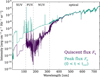 |
Fig. 3 Constructed flare event of Etot = 2 × 1033 erg, using the fiducial flare code of Loyd et al. (2018a) with δSi IV ≃ 105 s. We assume an instantaneous increase to the peak flux Fp (green) for the duration of tcol ≃ 2.2 × 10³ s, followed by an instantaneous decrease to the quiescent flux Fq (purple). |
3.2 Total flare energy
Flares cover a wide range of energies. The total radiative energy of a stellar flare can be evaluated by integrating the flux difference between the flaring and quiescent state over time and wavelength:
 (3)
(3)
Additionally, the equivalent duration δ gives the time interval it takes for the quiescent star to emit the same amount of energy as was released during the flare (Etot) and yields
 (4)
(4)
The GFE of AD Leo is estimated to have attained a total energy of ~1034 erg (Segura et al. 2010; Loyd et al. 2018b) across the entire measured wavelength domain. In this work, we first consider a flare that is roughly equally energetic in equivalent duration for GJ 876, which results in Etot = 2 × 1033 erg. Regarding radiative output in Si IV emission, the flare amounts to δSi IV ≃ 105 s. We show both the quiescent and peak SED of the Etot = 2 × 1033 erg flare in Fig. 3.
A well-established relation exists between the flare energy and frequency of occurrence. The flare frequency distribution (FFD) (e.g. Hawley et al. 2014; Davenport 2016) shows that high-energy flares are much less common than low-energy counterparts. Such a FFD is described by a power law
 (5)
(5)
where N(E) is the number of flares in a given time interval, E the flare energy, and α and k constants. Integrating this expression from E to infinity gives
 (6)
(6)
where ν denotes the flare frequency for flares with energies of E and higher. Loyd et al. (2018a) have found a striking similarity between the FFDs of inactive and active M dwarfs when computed with respect to equivalent duration instead of energy. The same conclusion is reached when differentiating M dwarfs with age (Loyd et al. 2018b). When converted to equivalent duration, the hypothetical 2 × 1033 erg flare of GJ 876, considered in this work, would occur roughly every 10 to 100 days. We note that a flare of 2 × 1033 erg, with an occurrence every 10 to 100 days, places this flare just in the superflare regime. We further explore the effects of repeated flaring and in Sects. 4.6 and 4.7.
4 Results
Throughout all the chemistry simulations performed in this study, we found that CH4, NH3, C2H2, and HCN are the best indicators of flare-induced photochemistry. This is in agreement with previous work that studied quiescent irradiation (e.g. Moses et al. 2011; Shulyak et al. 2020; Baeyens et al. 2022). Additionally, these constituents contribute substantially to the transmission spectrum. Therefore, we focus the discussion of our results on the evolution of the photochemically active species CH4, NH3, C2H2, and HCN to characterise the effects of the flare on the atmosphere. Other prominent constituents, such as H2O, CO2, and CO, are also affected but much less pronounced and are therefore only discussed briefly in Sect. 4.1 and appendices. We express abundances of species i in molar fraction, given by
 (7)
(7)
where n are number densities and N is the total number of atmospheric constituents.
4.1 Evolution of the chemical composition
Figure 4 shows the evolution of CH4, NH3, C2H2, and HCN at four longitudes (substellar and antistellar point, morning and evening limb) during the first ~2.3 days (Pwind/2) after the start of the flare event. The latter time interval is the time it takes for horizontal transport to advect the constituents of the flared dayside completely to the nightside in our model (Eq. (2)). Naturally, the substellar point shows the largest variations in response to the flare event. The upper atmosphere (p < 0.1 mbar) becomes depleted in NH3 and CH4 by several orders of magnitude with respect to the pre-flare steady-state. For example, at 1 μbar, φ (NH3) /φ(ss) (NH3) ≃ 6 × 10⁻³ and φ (CH4) /φ(ss) (CH4) ≃ 4 × 10⁻² where φ(ss) denotes the pre-flare, steady-state molar fraction. The dayside distribution of C2H2 is affected throughout almost the entire atmosphere by depletion (p < 1 μbar and 0.1 mbar < p < 0.1 bar) down to a factor 0.1 at ~0.1 μbar and by a slight enhancement (1 μbar < p < 0.1 mbar). Also HCN is photodissociated in the upper layers (p < 1 μbar), reducing φ(HCN) by a factor ~10 and slightly producing the constituent around ~10 μbar.
The evening limb distributions resemble the substellar point as a result of zonal advection that pollutes the terminator with the flared dayside. However, the evening limb only returns to it’s pre-flare composition after ~2.3 days, while the substellar point recovers much faster. Indeed, horizontal transport of un-flared nightside material reaches the substellar point after only ~28 h (Pwind/4) after which the periodic steady-state composition is again recovered. The evening limb remains in a perturbed state twice as long (Pwind/2) as it is supplied with flared dayside constituents from as far back as the morning limb. This also implies that the morning limb recovers very fast after the flare event. Indeed, the morning limb returns to its pre-flare distribution in merely ~2 h after the start of the flare event.
Although the flare event alters the molar fractions of above species by orders of magnitudes on the substellar point and evening limb, the antistellar point remains fairly unaffected. In a time interval of ~2.3 days, the substellar point constituents have been advected to the antistellar point. Upon entering the colder nightside, shielded from stellar irradiation, photodissociated methane and ammonia recombine and erase any traces of the initial depletion. The same does not hold for the molar fractions of acetylene and hydrogen cyanide, two species that are known to be produced from photodissociated CH4 and NH3 (Moses 2014). The nightside becomes slightly enriched with C2H2 and HCN up to a factor three, several days after the flare event.
Although during the first ~2.3 days after the start of the flare, the atmosphere’s response is most extreme, subtle leftovers can be seen long after the flare event. Figure 5 shows the molar fraction of C2H2 relative to its pre-flare value at different pressures in the atmosphere up to 2 weeks after the flare event. The nightside production of C2H2 persists within the first Pwind time interval throughout the entire vertical atmosphere, with the exception of the upper layers (0.1 μbar). As the enriched nightside is advected further eastwards, the substellar point becomes enhanced by a factor 2 (after ~4.6 days) and the evening limb by a factor 3 (after ~5.8 days) in the middle regions (10 μbar and 1 mbar). Furthermore, it is clear that the upper layers recover faster compared to regions of higher pressure. Indeed, the deep atmospheric layer at 0.1 bar experiences variations on the nightside distribution for over a week after the flare event.
We briefly mention the effect of the flare event on species other than NH3, CH4, C2H2, and HCN (see also Appendix A). In the upper layers (p < 1 μbar) of the dayside, H2, H2O, and CO2 become slightly depleted and CO marginally enhanced by less than an order of magnitude. The dayside hemisphere is enriched in atomic hydrogen by a factor ten up to pressures of ~ 1 bar and slowly regains its pre-flare molar fractions within a factor two after Pwind.
4.2 Evolution of the transmission spectra
In order to quantify the observational implications of variations in the chemical composition, we calculate transmission spectra during and after the flare event. Figure 6 shows the transmission spectrum of the evening and morning limb for the atmosphere with a pre-flare molecular composition. In Fig. 7, we compute spectra with atmospheric compositions perturbed by the flare (see Sect. 4.1) and subtract these from the pre-flare spectrum.
During the first few hours after the flare (0 < t ≲ 37 min), the evening limb transit depths decrease by less than 30 ppm for λ < 10 μm, mainly due to H2O depletion (with small contributions from depleted CH4 and NH3). At 14 μm, photodissociation of C2H2 reduces the transit depth by 100 ppm in a narrow spectral feature. Additionally, depletion of HCN leads to a broader region around 14 μm by less than 30 ppm reduction of the transit depth. This is in contrast to the morning limb, where acetylene production creates additional opacity and raises the 14 μm transit depth by 200 ppm. Furthermore, methane depletion decreases spectral features around 3.3 μm and 7.8 μm by 50-100 ppm while H2O (and NH3) affect the transmission spectrum with less than 20 ppm. As expected from the effects of horizontal transport, the evening limb does not show signs of recovery ~2 h after the start of the flare, while the morning limb has returned back to its pre-flare state in this time interval.
During the first Pwind time interval, a large discrepancy exists between the evening and morning limb evolution in time. As expected from the chemical response of the atmospheric constituents, the evening limb is perturbed up to ~2.3 days after the flare event. Methane depletion lowers the transit depths by up to 300 ppm (around 3.3 μm and 7.8 μm) while C2H2 production introduces additional opacity around 3 and 14 μm altering the spectrum up to 200 ppm. We note that the latter molecule now increases the transit depth on the evening limb, as opposed to the first few hours. The morning limb remains free from deviations during the first ~2.3 days, with the exception of the first hours after the flare. Afterwards, from ~2.3 to ~4.6 days, the roles reverse and the evening limb experiences no substantial deviations from the pre-flare state because, in this time interval, the constituents of the nightside are advected completely to the day-side again, crossing the morning limb. As shown in Sect. 4.1, C2H2 is produced substantially on the nightside. Subsequently, this enhancement is responsible for increasing the transit depths at 3 μm (~ 100 ppm) and 14 μπι (<350 ppm). The latter absorption feature consists of a broad band (~ 100 ppm) due to HCN production accompanied by the strong narrow peak of C2H2. Finally, for t > 4.6 days, C2H2 (and HCN) continues to temporarily enhance the transit depths, although by less than 20 ppm, when the flared dayside is again transported over the evening and morning limbs.
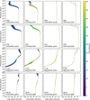 |
Fig. 4 Evolution of CH4, NH3, C2H2, and HCN (top to bottom) on the substellar point, evening limb, antistellar point and morning limb (left to right) during the first ~2.3 days (Pwind/2) after the flare event that started on t = 0. The pre-flare distributions are represented by the black dashed-dotted lines. |
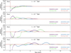 |
Fig. 5 Evolution of C2H2 in the first ~2 weeks after the flare event at different pressures in the atmosphere on four longitudes. By plotting different longitudes, we trace the advection of atmospheric constituents by the horizontal wind in time. |
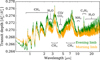 |
Fig. 6 Transmission spectra of the evening (green) and morning limb (orange) with the pre-flare molecular composition. The molecules that are predominantly responsible for certain absorption features are indicated on the relevant wavelength. |
4.3 Impact of different climates
Before exploring flares of different energies, we turn our attention to the factors that impact the climate of tidally locked gaseous exoplanets. In particular, the strength of equatorial superrotation and temperature structure play a crucial role in determining the spatial, steady-state distribution of molecular species (Baeyens et al. 2021). Therefore, we run two additional models with the same flare event of 2 × 1033 erg. First, we double uwind to 3.058 km s−1, while keeping other parameters fixed (run 1). Second, we consider another planet model of Baeyens et al. (2021) with Teff = 1600 K and set uwind = 1.529 km s−1 (run 2), the latter equalling the value adopted in previous runs (see Sects. 4.1 and 4.2). The model of run 2 has a two-dimensional temperature structure with a much stronger day-night gradient and also adopts different, generally higher, eddy diffusion coefficients. Additionally, the main carbon-bearing molecule in the pre-flare chemical composition is CO for models with Teff = 1600 K, compared to CH4 for Teff = 800 K. An effective temperature of 1600 K yields an orbital separation of 0.00296 AU, which affects the incident flux levels of stellar radiation. In this section, we refer to the nominal Teff = 800 K model with uwind = 1.529 km s−1, described in Sects. 4.1 and 4.2, as run 0. Additional differences between the set-ups of these runs are summarised in Table 1. For a detailed discussion on the differences between the pre-flare compositions of the models with Teff = 800 K (run 0 and run 1) and Teff = 1600 K (run 2), we refer to B22.
A selection of the results are shown in Figs. 8 and 9. In run 1, again two phases can be identified, before and after Pwind/2. There are only minor differences related to the amount of methane and ammonia depletion on the dayside (t < Pwind/2) and C2H2 and HCN production on the nightside (t > Pwind/2) (only C2H2 is shown). After multiple Pwind (which differs between run 0 and run 1, see Table 1) and thus multiple advection periods around the planet, the molar fractions of C2H2 also remain high compared to the pre-flare values. However, because  , this does not imply that the atmosphere in run 1 remained perturbed longer by the flare event. Instead, because horizontal transport is twice as fast, and the vertical mixing and chemical timescales remains fixed, more column rotations can be completed in the same time interval before the pre-flare distribution is recovered (Fig. 8). Therefore, we conclude that, in the case of a stronger zonal wind, the constituents of the flared dayside are circulated more times around the planet but the atmosphere’s response in time stays qualitatively the same.
For run 2 (Fig. 9), the atmosphere’s response to the flare event is predominately controlled by the differences with run 0 in orbital separation and planet temperature. Because this hypothetical planet is about four times closer than in run 0, the photochemical rates during the flare event are higher. Therefore, the depletion in the upper atmosphere of the dayside is much higher. More specifically; around ~1 μbar, φ (NH3) / φ(ss) (NH3) ≃ 10−3, φ (CH4) / φ(ss) (CH4) ≃ 3 × 10⁻⁴, φ (C2H2) / φ(ss) (C2H2) ≃ 2 × 10⁻⁴, and φ (HCN) / φ(ss) (HCN) ≃ 9 × 10⁻². Furthermore, a higher effective temperature of 1600 K implies that chemical equilibrium determines the composition down to a few mbar, while for Teff = 800 K (run 0) this was only the case for the deep layers (p > 1 bar). Given the short chemical timescales, the flare event does not substantially affect the middle/deep atmosphere in run 2. Aside from the differences originating in temperature and orbital separation, the atmosphere’s response to the flare event is qualitatively similar as in run 0 for the first ~2.3 days (Pwind/2) after the start of the flare. Although we do not show the evolution of the constituents after ~2.3 days, we report that the nightside becomes slightly enhanced in C2H2, as was also the case in run 0. However, we identify a striking difference in the evolution of the morning limb of run 2. When the constituents of the flared dayside are advected over the nightside towards the morning limb, we see little to no enhancement of C2H2 and HCN on the morning limb several days after the flare event. This is in contrast to the evolution of the model atmospheres with Teff = 800 K, where we find a substantial production of these species on the nightside that are subsequently advected several times across the planet. It thus seems that the hotter planet recovers its pre-flare composition in less than the Pwind time interval, and thus differs from the atmosphere’s response of the planet with Teff = 800 K. Although many aspects can contribute to this difference, we accentuate that the chemical timescales are shorter in warmer regimes, which supports a faster recovery after a perturbation such as a flare event. We discuss the evolution of the transmission spectra of run 2 in Appendix B.
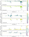 |
Fig. 7 Differences in the transmission spectra of the evening and morning limb with respect to the pre-flare state during the flare (lower), up to Pwind after the flare (middle) and up to 2 Pwind after the flare (upper). |
Parameters for the models with different climate conditions.
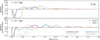 |
Fig. 8 Evolution of acetylene on different longitudes in the middle (1 mbar) and deep atmosphere (0.1 bar) for run 0 and run 1. We note that the horizontal axis is in units of Pwind, which differs between runs (see Table 1). |
4.4 Impact of total flare energy
We analyse the Teff = 800 K planet with uwind = 1.529 km s−1, and run the chemistry model with flares of different energies. We consider flares of energies Etot ∈ [2 × 1032,2 × 1033, 2 × 1034] erg, by scaling the peak flux Fp accordingly. The simulation with Etot = 2 × 1033 erg will be used as a baseline to compare other simulations with different Etot to, and we refer to Sects. 4.1 and 4.2 for a detailed discussion on this baseline model. Figure 10 shows the molar fractions of CH4, NH3, C2H2, and HCN throughout the ~ 1 month simulation domain. As expected, the overall impact of the 2 × 1032 erg flare is small, while the opposite holds for the 2 × 1034 erg flare. The latter causes more CH4 and NH3 depletion in the upper regions of the dayside and evening limb, as well as more production of HCN and C2H2 on the nightside and morning limb. For example, relative to the pre-flare composition, this quantifies as φ (NH3) φ(ss) (NH3) ≃ 10−5 and φ (CH4) /φ(ss) (CH4) ≃ 3 × 10⁻⁵ on the substellar point at 1 μbar. During the simulation with Etot = 2 × 1032 erg, the molar fractions of none of the species change by more than a factor 20 relative to their pre-flare values. Overall, variation of Etot results in a scaling of the depletion and enhancement patterns throughout the atmosphere compared to the case of Etot = 2 × 1033 erg. Thus the atmosphere’s response is qualitatively the same for flares of different energies. Also the spectral features that are affected in the evolution of the transmission spectra are qualitatively similar with respect to the case. The maximal variation in transit depth on the evening limb during 0 < t ≲ 2.3 days are 60 ppm and 800 ppm for flare energies of 2 × 1032 erg and 2 × 1034 erg respectively, compared to a value of 300 ppm for the baseline model of Etot = 2 × 1033 erg. For the morning limb during 2.3 days ≲ t ≲ 4.6 days, these numbers are 60 ppm and 700 ppm for flare energies of 2 × 1032 erg and 2 × 1034 erg, compared to 350 ppm for the baseline model.
4.5 Impact of flare duration
In Sect. 3.1, we adapted the fiducial flare code of Loyd et al. (2018a) such that all flares considered in this work last ~37 min (tcol) while in reality, the duration is correlated to the energy and can range from minutes to hours (e.g. Walkowicz et al. 2011; Hawley et al. 2014; Seli et al. 2021; Bourrier et al. 2021; Jackman et al. 2021b). Therefore, we aim to explore if the flare duration has a substantial impact on the atmosphere’s response by comparing the previous results to long duration flares. We follow Chadney et al. (2017) in taking a simplified approach for the time evolution by considering an instantaneous increase to the peak flux Fp, followed by an exponential decay towards quiescence Fq. The time-dependent stellar flux can then be expressed as
 (8)
(8)
with f(t) = exp(−ηt) and η a constant determined by the duration of the flare, assuming that the flare happens at t = 0. We note that the difference with the previous flare is that after the first column integration (0 < t < tcol), the flux decreases exponentially to quiescence rather that instantaneously, although the exponential decay still happens in time-steps of tcol. Following the duration of the GFE of AD Leo, we consider a duration of ~4h by setting η = 1.727 so that f(t = 4 h) = 10−3 (Eq. (8)). To conserve an integrated total energy of 2 × 1033 erg for a duration of 4 h, we scale the peak flux to ~65% of its initial value (shown in Fig. 3). This implies that the remaining ~35% is included in the exponential decay. Furthermore, we construct flares with a duration of 2 and 8 h for which we adopt a value for η of 3.454 and 0.863 respectively. This implies that the peak flux must be ~83% and ~40% of the initial value (Fig. 3) for the flares of 2 and 8 h respectively to amount to an energy of 2 × 1033 erg.
In Fig. 11, we show the evolution of CH4 and NH3 during the first ~2.3 days (PWind/2) after the start of the flare event in the upper atmosphere (1 μbar) of the evening limb. Although the differences between these runs are rather subtle, we find that the effect of the flare duration manifests itself in a number of ways. Firstly, the curves corresponding to long duration flares (e.g. 8 h) are elongated to the right on the horizontal time-axis, which results from a slower decrease to quiescence compared to shorter flares. Secondly, flares with longer duration seem to deplete the evening limb more in CH4 and NH3 than shorter flares after advection across the dayside from ~1 day onwards, although this effect seems limited to a factor two. Interestingly, the lower value of the peak flux for longer flares does not seem to play a significant role compared to the duration of the exponential decay. Due to the lack of diffusive mixing in the longitudinal direction in our models, the above effects do not dissipate and last throughout the entire simulation but remain relatively small.
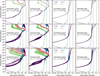 |
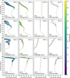
Fig. 10 Distributions of CH4, NH3, C2H2, and HCN during and ~1 month after a flare event of total energy 2 × 1032 erg (upper row), 2 × 1033 erg (middle row) and 2 × 1034 erg (lower row). From left to right: substellar point, evening limb, antistellar point and morning limb. The pre-flare distributions are represented by the black dotted lines. |
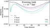 |
Fig. 11 Evolution of CH4 and NH3 during the first ~2.3 days (PWind/2) after the start of the flare event in the upper atmosphere (1 μbar) of the evening limb. Three simulations are shown that correspond to 2 × 1033 erg flares of 2 (dashed-dotted), 4 (dashed) and 8 (dotted) hours. The simulation discussed in Sects. 4.1 and 4.2, with a flare of tcol without exponential decay, is shown by the solid line. |
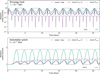 |
Fig. 12 Evolution in time during the entire ~1 month simulation span of CH4 and NH3 at 1 μbar on the evening limb (upper panel) and HCN and C2H2 at 1 mbar on the antistellar point (lower panel). Three runs are shown where a 2 × 1033 erg flare event occurs every 1 day (dashed), 2.3 days (Pwind/2; solid) and 4.6 days (Pwind; dotted). |
4.6 Impact of repeated flaring
Flares do not occur once in the lifetime of a star. Instead, exoplanetary atmospheres will be flared repeatedly with a frequency that correlates with the total radiative output of the flare (Etot). In this section, we explore the effects of repeated flaring in a simplified way by only considering 2 × 1033 erg flares, thereby omitting the inclusion of a FFD. However, we consider the possible effects of such a FFD later in this paper (Sect. 4.7). For now, we consider flare periods of 1 day, 2.3 days (PWind/2) and 4.6 days (Ρwind).
Figure 12 shows the evolution of CH4 and NH3 in the upper region (1 μbar) of the evening limb, and of HCN and c2h2 in the middle layers (1 mbar) of the antistellar point. When the flare period equals 4.6 days, the atmosphere fully recovers to its pre-flare molar fraction between consecutive flare events. This is, however, not the case when the flare period equals 1 day. Instead, the continuously flared atmosphere maintains a perturbed state after 2–3 events, around which the molar fractions fluctuate. For example, NH3 remains depleted by over an order of magnitude relative to its pre-flare value. Although initially it takes several days to reach this new state, there does not seem to be a cumulative effect over longer timescales to which the atmosphere is continuously evolving towards. The transition between these two regimes occurs when a flare period of 2.3 days is adopted. In our model, it takes 2.3 days or PWind/2 to horizontally transport the entire flared dayside to the nightside. In that same time interval, the unaffected nightside is now advected completely to the day-side. Therefore, a new flare hitting the dayside after 2.3 days does not build on the effects of its precursor. We nuance and discuss the validity of this result further in Sect. 5.2.5. Finally, we echo that a 2 × 1033 erg flare on GJ 876 would occur roughly every 10–100 days (Sect. 3.2) and that a flare period of less than a week is unlikely. However, we adopt the above flare periods to illustrate the boundary between lasting and non-lasting damage to the atmosphere, within the context of the adopted chemistry model.
4.7 Impact of a flare frequency distribution (FFD)
Finally, we consider a more realistic case of repeated flaring by considering a range of flare energies and occurrences that adhere to a FFD. We use the fiducial flare code of Loyd et al. (2018a) to generate such a FFD that is shown in Fig. 13. The constructed FFD lasts about 2 weeks and all individual flares have a duration Of tcol.
Figures 14 and 15 show the variation in molar fraction compared to the pre-flare composition for CH4, NH3, C2H2, and HCN on the substellar and antistellar point respectively. The results are in line with what we expect from the previous simulations, namely that mainly the upper atmosphere of the dayside is affected and the nightside become slightly enhanced with C2H2 and HCN. Interestingly, the combination of high- and low-energy flares seems to keep the atmosphere in a composition that differs from pre-flare values, although there are clear fluctuations around this post-flare state. To quantify these fluctuations, we can compute the median values for the abundances of certain molecules for different points in the atmosphere. At 1 μbar on the substellar point, the median molar fraction of CH4 is about a factor five lower than before the flaring and a factor ~15 for NH3. We show the evolution of other species in Appendix C.
The FFD clearly manages to drive the atmospheric composition away from its pre-flare, steady-state distribution. As shown in Sect. 4.2, we expect the perturbed composition to affect the transmission spectrum on different wavelengths, mainly due to CH4 depletion on the evening limb and C2H2 production on the morning limb. Figure 16 shows the transmission spectra on every time-step during the simulation with FFD flaring, superimposed onto each other. At several wavelengths, the transit depths do not return to the pre-flare values during the simulation. Around 2.2 μm, 3.3 μm, and 7.8 μm, CH4 decreases the median transit depth by 100 to 200 ppm on the evening limb, while C2H2 increases the median value up to 500 ppm at 3 μm and 14 μm on the morning limb. As will be discussed in Sect. 5.3.1, this result has important implications for future observations of similar close-orbiting planets around active stars.
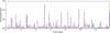 |
Fig. 13 Light-curve of the adopted FFD in the Si IV doublet line (1393 Å). The plotted flux is normalised to the quiescent value. |
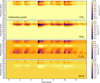 |
Fig. 14 Evolution of CH4, NH3, C2H2, and HCN throughout the vertical atmosphere on the substellar point during ~two weeks of continuous flaring according to a FFD. The colourbar denotes the logarithm of the ratio between the current (φ) and the pre-flare, steady-state composition (φ(ss)). |
5 Discussion
5.1 Comparison to previous work
5.1.1 Venot et al. (2016)
As mentioned in Sect. 1, Venot et al. (2016) (V16 hereafter) have studied the consequences of a stellar flare on a sub-Neptune (Teff = 1303 K) and super-Earth (Teff = 412 K). To describe the flare event, they used a time series based on the GFE of AD Leo that was constructed from observations by Segura et al. (2010). The synthetic flare event used in this work contains a similar radiative output, relative to the quiescent flux levels, so that both equivalent durations are comparable (Sect. 3.2). Therefore, the results of V16 can best be compared to the outcomes of our models where Etot ≃ 2 × 1033 erg. Additionally, V16 used a one-dimensional photo- and thermochemical model to study the neutral composition, in which they use the chemical network of Venot et al. (2012). Aside from differences in thermal background structure, vertical mixing coefficients, planetary and stellar input radii/masses, etc., we model the longitudinal dimension with Agúndez et al. (2014)’s pseudo-2D model and include the updated chemical network of Venot et al. (2020a). Taking into account these differences between our work and the study of V16, only a qualitative comparison of the atmosphere’s response can be drawn.
V16 found that the upper layers (<1 μbar) of the super-Earth are depleted in ammonia by up to a factor ~20 during the flare event, while the sub-Neptune becomes enriched by a factor ~15. For none of the different climates we considered (Sect. 4.3), do we find any compelling production of ammonia. Furthermore, we find that the initial depletion of NH3 on the dayside during the flare event ranges from a factor 200 (run 0, Sect. 4.3) to 1000 (run 2, Sect. 4.3). We thus generally find a higher ammonia depletion by at least on order of magnitude, compared to V16. For example, we note that our pre-flare compositions differ from V16 as both their planets are subjected to high quiescent (X)UV-flux from the extremely active AD Leo, which already deprives the upper layers from photochemically reactive species such as ammonia. Although we have focused mostly on four photochemically active molecules in this work, other species that are generally less affected such as CO, CO2, NH2, H, and OH are qualitatively impacted in similar ways (on the dayside) as in the models of V16.
V16 also addressed the implications on the transmission spectrum of the planet and found that mainly the co2 features at 4.6 and 14 μm are affected during the flare event. This is in stark contrast to what we find, namely that the CH4 and C2H2 opacities impact the morning and evening limb during the flare event. A possible explanation for this is the discrepancy in pre-flare spectra, as this determines the relative sensitivity of the transit depths during a perturbation such as a flare event. V16 found pronounced CO2 features in the pre-flare transmission spectra of both their models, while we do not reproduce this. The prevailing spectral feature of CO2 is likely a direct result of the high average molar fraction (~10−4) that they compute in their pre-flare composition. The pre-flare chemical state that we compute in this work and in B22 is much less rich in CO2 (φ ≃ 10−7). We note that V16 did not include C2H2 in their radiative transfer calculations (only H2O, CO2, OH, HCN, CH4, and CO).
Finally, V16 also found that a single flare event can force the atmosphere to a new, post-flare chemical composition that converges to anew steady-state after ~30000 yr. This renewed state of the atmosphere then differs in the transmission spectra around 4.6 and 14 μm (again CO2-features) by ~40 ppm and ~500 ppm for the super-Earth and sub-Neptune, respectively. The value for the latter planet can reach up to 1200 ppm when the atmosphere is flared every ~5 h. V16 explained this phenomenon by hypothesising that a flare permanently modifies the photochemical rates so that the upper atmosphere is effectively bleached by the flare. They further suggested that the lower layers maintain this new level of transparency long after the star returns to quiescence, which exposes the underlying layers to more intense radiation. Although we are not able to extend our models to ~30000 yr due to the linearity between physical and computation time (see Eq. (1)), we do not expect to find a post-flare composition that differs substantially from the pre-flare state. By considering horizontal transport in our work, we effectively introduce an additional degree of freedom that is not present in the models of V16. The fact that all of our single flare models have fully recovered their pre-flare composition by the end of our simulation time-domain (~ 1 month), and even recover within a factor five after one week, is in line with what we would expect from a realistic atmosphere when no other chemical sources or sinks are present compared to the pre-flare conditions. A quantitative comparison and chemical pathway analysis between two models could further clarify the discrepancy.
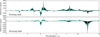 |
Fig. 16 Differences in transmission spectra with respect to the pre-fiare state on every time-step during the ~two weeks of flaring according to a FFD, superimposed onto each other in green. The median value of the transit depth on every wavelength is indicated in black. |
5.1.2 Louca et al. (2022)
Louca et al. (2022; L22 hereafter) considered three H2-dominated planet atmospheres of GJ 876c, GJ 832c, and GJ581c, with host stars that have been observed in the MUSCLES survey (France et al. 2016). They subsequently used the fiducial flare code of Loyd et al. (2018a) to generate FFDs and model the one-dimensional atmospheric composition. They find that the abundances of several species including CH4, CO, and H2O do not recover to pre-flare values in between subsequent flares and some even accumulate gradually over time. Based on the result presented in Sect. 4.7, we also find that several molecules (e.g. H, CH4) stay in a perturbed state with median molar fractions differing from the pre-flare values. However, for none of the species considered in this work, we see a clear trend that points to the accumulation in time. It can be argued that the horizontal transport prevents the atmosphere from accumulating flare effects by continuously replenishing the dayside with material from the nightside. Furthermore, L22 do not find that the changes in chemical composition affect the transmission spectra by more than several ppm, which is in contrast to what we find (see Fig. 16). Just like the discrepancy with V16, a more detailed comparison of the pre-flare conditions and model set-up is needed to further investigate these differences.
5.2 Model improvements and future work
5.2.1 Stellar particle events
Stellar flares are often accompanied by SPEs that eject (charged) energetic particles into space. Such SPEs can impact a planetary atmosphere by inducing additional photochemistry (Segura et al. 2010), enhancing ionization levels (Barth et al. 2021), and increasing mass-loss rates (Chadney et al. 2017). Because chemical models of planetary atmospheres that undergo SPEs have mainly been constructed to investigate the consequences on habitability (e.g. Segura et al. 2010; Tabataba-Vakili et al. 2016; Tilley et al. 2019; Atri 2020), little attention has been given to close-orbiting gaseous planets. A follow-up study, that assesses the combined effects of flares and SPEs on the chemical composition of such gas giants with a multi-dimensional kinetics model, would therefore be valuable.
5.2.2 Temperature structure
Throughout the chemistry simulations, we have fixed the thermal background to the two-dimensional distribution as was calculated for steady-state conditions by Baeyens et al. (2021). However, the temperature distribution might be affected during a flare event by the sudden increase of irradiation, change in chemical composition and even accompanying SPE. Although Segura et al. (2010) found that the temperature profile is perturbed by only a few Kelvin during and after a flare event of this magnitude, Venot et al. (2016) correctly argued that the radiative response of an atmosphere to a stellar flare will be much different for warmer, gaseous planets. More research is needed to properly assess the impact of a flare on the temperature structure of, for instance, an 800 K planet such as considered in this work.
5.2.3 Clouds and haze
We have neglected clouds and haze in our chemistry simulations and calculations of transmission spectra to isolate flare-induced changes to gas-phase molecules. However, aerosols are thought to be present in the bulk of exoplanet atmospheres (e.g. Marley et al. 2013; Gao et al. 2021). Therefore, we must place the findings presented in this work in the context of cloudy and hazy atmospheres.
Aerosols are likely to play an important role in the heat distribution of planets by back-warming the atmospheric layers below the cloud deck (greenhouse effect), and by increasing the albedo and thereby changing the incoming radiative energy (Helling 2019; Gao et al. 2021). The question then arises whether clouds can effectively lower photolysis rates on exoplanets by shielding the atmosphere from radiation, as has been shown for Earth’s atmosphere (Hall et al. 2018). Although it has not been modelled for exoplanet atmospheres, this effect could moderate the flare-impact on the molar fractions of photochemically active species.
Depending on the altitude of the aerosols, clouds and haze can also be responsible for flattening molecular absorption features in the transmission spectra of planets (e.g. Pont et al. 2008; Bean et al. 2010; Kreidberg et al. 2014). Although aerosols mainly affect the optical regime through Rayleigh scattering, the entire wavelength range can be affected depending on the particle size, composition and altitude of the aerosols (Gao et al. 2021). This could have implications on the values for flare-induced fluctuations in the transmission spectrum, reported in this work.
Finally, we have found that flares can increase molar fractions of hydro-carbons when photodissociated species from the dayside enter the nightside through horizontal transport. In particular, C2H2 is a precursor of more complex hydrocarbons and leads to haze formation. It is unclear how such a short-term perturbation to the gas-phase chemistry affects haze formation and whether this may introduce additional variations to the (optical) transit depths.
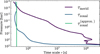 |
Fig. 17 Zonal (τzonal) and meridional (τmerid) advection timescale computed from the GCM outcome of the model planet corresponding to Teff = 800 K with a M dwarf host star, presented in Baeyens et al. (2021). An approximate zonal timescale |

5.2.4 Three-dimensional circulation
The climates of tidally locked, close-orbiting gaseous planets are three-dimensional, and aside from equatorial superrotation, their circulation pattern consists of a variety of flows. The equatorial middle layers (~1 bar to ~1 mbar) develop strong prograde winds, while a combination of pro- and retrograde flows is typically present at higher altitudes (≲0.1 mbar). The upper boundary of general circulation models typically ranges between 0.1 mbar and 1 μbar, to avoid numerical issues. Therefore, we are limited in information about the layers above these pressure values, which are generally of most interest for photochemistry. Some three-dimensional models of hot Jupiter exhibit jet streams that diminish in speed near the upper atmosphere (Cooper & Showman 2005, 2006; Rauscher & Menou 2010; Mayne et al. 2014), whereas other models sustain a superrotating jet stream up to the upper boundary of the simulation domain (Showman et al. 2009; Amundsen et al. 2016; Deitrick et al. 2020; Drummond et al. 2020; Schneider et al. 2022). Possible reasons for this discrepancy may be the radiative scheme (see discussion in Appendix D of Schneider et al. 2022) or the upper boundary treatment. In this work, we have assumed that horizontal winds dominate the entire equatorial band, including the upper layers down to 10−8 bar. To quantify the validity of this assumption, we use timescale arguments based on the GCM outcome of the model planet corresponding to Teff = 800 K with a M dwarf host star, presented in Baeyens et al. (2021). In particular, we compute the meridional advection timescale  with υ the meridional wind speeds and the zonal advection timescale
  with u the zonal wind speeds (Drummond et al. 2020). Both values are averaged over all longitudes and the equatorial latitudes (−20° < ϕ < 20°) and are shown in Fig. 17. The fact that τzonal ≪ τmerid for pressures above ~0.1 mbar illustrates that our assumption, that horizontal winds dominate the circulation pattern, is valid for the middle and deep atmosphere (down to ~0.1 mbar). Only in the uppermost regions does meridional advection become equally or more important than horizontal transport. However, the flare impacts these upper layers the most (e.g. Fig. 4) and it is possible that the inclusion of more detailed flows will impact our findings considerably.
At lower and higher latitudes (|ϕ| ≳ 50°) there can even be direct day-to-night flows over the poles at high altitudes. Both the equatorial meridional advection and polar day-to-night flows at high altitudes are likely to also impact the atmosphere’s recovery after a flare event by transporting and mixing material away from the flared dayside.
5.2.5 Superrotation as advection
The premise of the pseudo-2D chemistry model of Agúndez et al. (2014) is that equatorial superrotation can be approximated by a uniform zonal wind that acts as advection on the entire atmospheric column (solid-body rotation). Aside from reducing the complex three-dimensional circulation pattern to the dominating jet stream (see Sect. 5.2.4), the assumption of solid-body rotation with a fixed period Pwind (~4.6 days) is clearly a determining factor in our models for the evolution of the atmospheric composition after the flare event (e.g. Figs. 4, 5, 8). We found that the evening limb is perturbed in the first ~2.3 days (Pwind/2) after the start of the flare, while the morning limb remains unaffected several hours after the event. Between ~2.3 to ~4.6 days, the morning limb becomes affected while the evening limb fully recovers. However, this abrupt transition at Pwind/2 is an artefact of the chemistry model, and we do not expect such a time evolution in reality. Instead, additional processes such as small-scale turbulence and non-zonal mixing (see Sect. 5.2.4), will initiate further mixing of atmospheric layers. As such, we expect diffusion to modulate the patterns that we obtain from our purely advective models. Therefore, one should consider this transition value of Pwind/2 as an estimate, rather than a exact quantity. The same nuance holds for the results presented in Sect. 4.6, where we found that repeated flaring only manages to permanently perturb the atmosphere to a post-flare state when the flare period equals Pwind/2 or less.
5.2.6 Three-dimensional transmission spectroscopy
The transmission spectra presented in this work are computed with a thermal structure and molecular composition representative for the equator. However, transit spectroscopy probes the full terminator of the projected planetary disk, so the information from higher latitudes is missing from our models. Nevertheless, the equatorial region, which is generally hotter than the polar regions, is expected to dominate the spectral signature (e.g. Caldas et al. 2019; Baeyens et al. 2021).
Additionally, in this work, we focussed on flare-induced variations to the morning and evening limb separately, while both would contribute to the transmission spectra. The values reported in this work for flare-induced fluctuations on individual terminators are therefore likely upper limits as actual observations will be an average between the evening and morning limb contributions. We note that recently the ingress and egress of transiting exoplanets have been probed separately (Ehrenreich et al. 2020; Espinoza & Jones 2021), which provide unique insights on the three-dimensional structure of exoplanets. Finally, we note that recent studies which have researched asymmetries in three-dimensional transmission spectra indicate that the vertically extended evening limb contributes more than the less extended morning limb (Caldas et al. 2019; Falco et al. 2022; Pluriel et al. 2022; Lee et al. 2022; MacDonald & Lewis 2022; Nixon & Madhusudhan 2022).
5.3 Implications for observations
5.3.1 Additional uncertainty to JWST data
Considering our finding that repeated flaring according to a FFD can induce >50−100 ppm variations in the transmission spectra of the modelled close-orbiting gaseous planet(s), one can wonder what the implications are for the James Webb Space Telescope (JWST) that is estimated to achieve a similar precision (Barstow et al. 2015; Greene et al. 2016). In particular, repeated flaring could introduce an additional component of uncertainty to JWST data and may even result in measurable variability. Indeed, Fig. 16 indicated that the 3.3 μm CH4-feature and 14 μm C2H2-feature experience fluctuations of 100 to 300 ppm around a median transit depth. Such fluctuations could introduce an uncertainty to the observations of JWST, which in turn propagate into uncertainty on the retrieved abundances of CH4, C2H2, and potentially other species as well. Furthermore, the median transit depths of the before mentioned spectral features also differ by several hundreds of ppm from the values obtained when assuming stellar quiescence. This indicates that, if one does not account for flaring of the active host star during the analysis, one might bias the retrieved abundances. In order to quantify the above effects, one should perform retrievals on the computed transmission spectra, but this is out of scope for this work. In order to account for such changes in the modelling of planets around active stars, we consider it beneficial to monitor the planet’s host star in the UV up to several days before and during the scheduled planet observations.
In Sect. 4.6, we have also investigated repeated flaring for an extreme case of frequent high energy flares, and found that the atmosphere almost completely returns to its pre-flare state when the flare period is longer than a few days (i.e. Pwind/2 or 2.3 days for the considered model). The above conjecture heavily depends on Pwind, and by extension τzonal, which varies among planets with different climates, but is generally on the order of several days. Although we have nuanced the importance of the Pwind parameter in our chemistry models in Sect. 5.2.5, and investigated the effects of repeated flaring for a more realistic case by means of a FFD (Sect. 4.7), this result indicates that τzonal can be a valuable parameter in assessing how efficient the atmosphere recovers in between subsequent flare events.
Finally, Baeyens et al. (2022) have noted that photochemical processes have a limited impact on transit spectra in general, but high-resolution observations of exoplanet atmospheres are more likely to be affected by photochemistry. Therefore, we stress that any transmission-spectroscopic effects of flaring discussed in this work are potentially even more pronounced in high-resolution spectra.
5.3.2 High-cadence monitoring of active host stars
We have shown that both the flare’s total outputted radiative energy (Sect. 4.4) and exponential decay from peak to quiescence (Sect. 4.5) are important factors that control the impact on the planetary atmosphere. Current flare observations often have a poor time-sampling as a result of low-cadence monitoring, which can result in a degeneracy between sharply peaked and weakly peaked flares (Howard & MacGregor 2022), thereby losing critical information. Therefore, we advocate for high-cadence observations, such as the TESS 20-second cadence mode, for future monitoring of active host stars.
6 Conclusions
We have studied the effect of stellar flares on the chemical composition of a Teff = 800 K, tidally locked gaseous exoplanet. By combining a series of pseudo-2D chemistry models, we track the evolution of the two-dimensional molecular composition around the equatorial band, where the climate is dominated by a jet stream of ~1.5 km s−1 that advects an air parcel around the planet in ~4.6 days (Pwind). Simultaneously, we compute one-dimensional transmission spectra on both the evening and morning limb to assess the impact of fluctuations in the chemical composition. We have constructed a ~37 min flare of Etot 2 × 1033 erg from the SED of GJ 876 as a vantage point to explore flares that vary in total energy, duration, and occurrence frequency. We find that photochemically active and abundant species such as CH4, NH3, C2H2, and HCN are affected throughout the atmosphere. Furthermore, we show that, after a single flare event, the evening limb remains in a perturbed state until ~2.3 days (Pwind/2) after the start of the flare event, as then the flared dayside is completely advected to the nightside. Further advection from ~2.3 to ~4.6 days enhances the morning limb with C2H2 and HCN, which are produced by photodissociated ammonia and methane on the nightside (Moses 2014). We find that mainly methane depletion on the evening limb reduces transit depths by 100 to 300 ppm (t < 2.3 days) and acetylene production on the morning limb increases the 14 μm feature up to 300 ppm (2.3 days < t <4.6 days). After ~4.6 days, we see that C2H2 is advected with slightly enhanced molar fractions around the planet for up to two weeks after the flare event, mainly in the deeper layers (e.g. at 1 mbar), although this affects the spectra by less than 20 ppm. Because the three-dimensional circulation pattern of our hypothetical planet is simplified to a uniform zonal wind that advects an air parcel in exactly ~4.6 days, we argue that the above timeline, and in particular the transition on ~2.3 days, should be considered an estimate rather than an exact value.
A flared planet with effective temperature of 1600 K, that orbits closer to the star, experiences more depletion on the dayside in the upper atmosphere, is affected less deep in the vertical atmosphere due to shorter chemical timescales and recovers faster than the 800 K planet. After examining a variety of flares, we identify that flares of different energy change the atmosphere’s chemical response only quantitatively, and not qualitatively, and that longer duration flares seem to have a slightly larger impact due to their prolonged exponential decay. Both the importance of total radiative output and time evolution from peak to quiescence illustrate the need for high-cadence monitoring of active host stars. By considering multiple flare events following a FFD, we have shown that repeated flaring has the potential to permanently alter the chemical composition at several locations in the atmosphere. Furthermore, depletion of methane on the evening limb and production of acetylene on the morning limb can permanently alter the transit depth at wavelengths such as 3.3 and 14 μm by several hundreds of ppm, with fluctuations in the range from 100 to 300 ppm. We argue that the above effects have important implications for observations that will be acquired with JWST. Detectable variations in photochemically active molecules can be expected, and their retrieved abundances could be biased if flaring of the host star is not accounted for. Therefore, we recommend that transmission studies with JWST are accompanied and even preceded by simultaneous (UV) observations of the host star to further clarify the exoplanet’s atmospheric response to flaring.
Acknowledgements
The authors thank Marcelino Agundez for the use of the pseudo-2D chemistry code and Parke Loyd for creating the open source fiducial flare model. We also thank the referee for their insightful comments that highly improved this work. T.K., R.B., and L.D. acknowledge support from the KU Leuven IDN grant IDN/19/028. R.B. acknowledges funding from a PhD fellowship of the Research Foundation - Flanders (FWO). R.B. and L.D. acknowledge support from the FWO research grant G086217N.
Appendix A Evolution of constituents not discussed in Sect. 4.1
To provide full transparency regarding the behaviour of other prominent species that were not discussed in Sect. 4.1, we show the evolution of CO2, H2O, H, OH, and NH2 during the first ~2.3 days (Pwind/2) after the flare event in Fig. A.1.
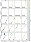 |
Fig. A.1 Same as Fig. 4, but for CO2, H2O, H, OH, and NH2. We note that the range on the horizontal axis is now extended to lower molar fractions. |
Appendix B Transmission spectra of run 2 (Sect. 4.3)
We briefly discuss the evolution of the transmission spectra during and after the flare event of run 2 (planet model with Teff = 1600 K and Pwind = 4.6 days; see Table 1) based on Fig. B.1. In contrast to the flare simulations on the Teff = 800 K planet, we see that mainly H2O affects the transmission spectrum in the first ~4.6 days after the flare. Additionally, production of OH impacts the spectrum above ~15 μm. After ~4.6 days (not shown), the spectrum is altered by less than ~20 ppm, which is in agreement with our finding that the chemical composition returns to its pre-flare values almost completely within the Pwind time interval.
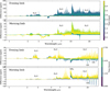 |
Fig. B.1 Differences in the transmission spectra of the evening and morning limb with respect to the pre-flare state during the flare (lower) and up to Pwind after the flare (upper) for run 2 of Sect. 4.3. |
Appendix C Evolution of constituents not discussed in Sect. 4.7
To provide full transparency regarding the behaviour of other prominent species that were not discussed in Sect. 4.1, we show the evolution of CO2 , H2O, H, OH, and NH2 throughout the vertical atmosphere on the substellar (Fig. C.1) and antistellar point (Fig. C.2) during ~two weeks of continuous flaring according to a FFD.
References
- Agúndez, M., Parmentier, V., Venot, O., Hersant, F., & Selsis, F. 2014, A&A, 564, A73 [Google Scholar]
- Amundsen, D. S., Mayne, N. J., Baraffe, I., et al. 2016, A&A, 595, A36 [NASA ADS] [CrossRef] [EDP Sciences] [Google Scholar]
- Atri, D. 2017, MNRAS, 465, L34 [NASA ADS] [CrossRef] [Google Scholar]
- Atri, D. 2020, MNRAS, 492, L28 [NASA ADS] [Google Scholar]
- Baeyens, R., Decin, L., Carone, L., et al. 2021, MNRAS, 505, 5603 [NASA ADS] [CrossRef] [Google Scholar]
- Baeyens, R., Konings, T., Venot, O., Carone, L., & Decin, L. 2022, MNRAS, 512, 4877 [NASA ADS] [CrossRef] [Google Scholar]
- Barstow, J. K., Aigrain, S., Irwin, P. G. J., Kendrew, S., & Fletcher, L. N. 2015, MNRAS, 448, 2546 [NASA ADS] [CrossRef] [Google Scholar]
- Barth, P., Helling, C., Stüeken, E. E., et al. 2021, MNRAS, 502, 6201 [Google Scholar]
- Bean, J. L., Miller-Ricci Kempton, E., & Homeier, D. 2010, Nature, 468, 669 [NASA ADS] [CrossRef] [Google Scholar]
- Bellotti, S., Petit, P., Morin, J., et al. 2022, A&A, 657, A107 [NASA ADS] [CrossRef] [EDP Sciences] [Google Scholar]
- Benz, A. O., & Güdel, M. 2010, ARA&A, 48, 241 [NASA ADS] [CrossRef] [Google Scholar]
- Bochanski, J. J., Hawley, S. L., Covey, K. R., et al. 2010, AJ, 139, 2679 [NASA ADS] [CrossRef] [Google Scholar]
- Boisse, I., Bouchy, F., Hébrard, G., et al. 2011, A&A, 528, A4 [NASA ADS] [CrossRef] [EDP Sciences] [Google Scholar]
- Bourrier, V., dos Santos, L. A., Sanz-Forcada, J., et al. 2021, A&A, 650, A73 [NASA ADS] [CrossRef] [EDP Sciences] [Google Scholar]
- Bruno, G., Lewis, N. K., Valenti, J. A., et al. 2022, MNRAS, 509, 5030 [Google Scholar]
- Caldas, A., Leconte, J., Selsis, F., et al. 2019, A&A, 623, A161 [NASA ADS] [CrossRef] [EDP Sciences] [Google Scholar]
- Cauley, P. W., Kuckein, C., Redfield, S., et al. 2018, AJ, 156, 189 [Google Scholar]
- Chadney, J. M., Koskinen, T. T., Galand, M., Unruh, Y. C., & Sanz-Forcada, J. 2017, A&A, 608, A75 [NASA ADS] [CrossRef] [EDP Sciences] [Google Scholar]
- Charbonneau, D., Brown, T. M., Noyes, R.W., & Gilliland, R. L. 2002, ApJ, 568, 377 [NASA ADS] [CrossRef] [Google Scholar]
- Chebly, J. J., Alvarado-Gómez, J. D., & Poppenhaeger, K. 2022, Astron. Nachr., 343, e10093 [NASA ADS] [CrossRef] [Google Scholar]
- Chen, G., Pallé, E., Welbanks, L., et al. 2018, A&A, 616, A145 [NASA ADS] [CrossRef] [EDP Sciences] [Google Scholar]
- Chen, H., Zhan, Z., Youngblood, A., et al. 2021, Nat. Astron., 5, 298 [Google Scholar]
- Christie, D. A., Mayne, N. J., Lines, S., et al. 2021, MNRAS, 506, 4500 [CrossRef] [Google Scholar]
- Collier Cameron, A., Ford, E. B., Shahaf, S., et al. 2021, MNRAS, 505, 1699 [NASA ADS] [CrossRef] [Google Scholar]
- Colombo, S., Pillitteri, I., Orlando, S., & Micela, G. 2022, Astron. Nachr., 343, e10096 [NASA ADS] [CrossRef] [Google Scholar]
- Cooper, C. S., & Showman, A. P. 2005, ApJ, 629, L45 [NASA ADS] [CrossRef] [Google Scholar]
- Cooper, C. S., & Showman, A. P. 2006, ApJ, 649, 1048 [CrossRef] [Google Scholar]
- Davenport, J. R. A. 2016, ApJ, 829, 23 [Google Scholar]
- Davenport, J. R. A., Becker, A. C., Kowalski, A. F., et al. 2012, ApJ, 748, 58 [NASA ADS] [CrossRef] [Google Scholar]
- Deitrick, R., Mendonça, J. M., Schroffenegger, U., et al. 2020, ApJS, 248, 30 [NASA ADS] [CrossRef] [Google Scholar]
- Dobrijevic, M., Hébrard, E., Loison, J. C., & Hickson, K. M. 2014, Icarus, 228, 324 [NASA ADS] [CrossRef] [Google Scholar]
- Drummond, B., Tremblin, P., Baraffe, I., et al. 2016, A&A, 594, A69 [NASA ADS] [CrossRef] [EDP Sciences] [Google Scholar]
- Drummond, B., Hébrard, E., Mayne, N. J., et al. 2020, A&A, 636, A68 [NASA ADS] [CrossRef] [EDP Sciences] [Google Scholar]
- Dumusque, X. 2018, A&A, 620, A47 [NASA ADS] [CrossRef] [EDP Sciences] [Google Scholar]
- Ehrenreich, D., Lovis, C., Allart, R., et al. 2020, Nature, 580, 597 [Google Scholar]
- Espinoza, N., & Jones, K. 2021, AJ, 162, 165 [NASA ADS] [CrossRef] [Google Scholar]
- Falco, A., Zingales, T., Pluriel, W., & Leconte, J. 2022, A&A, 658, A41 [NASA ADS] [CrossRef] [EDP Sciences] [Google Scholar]
- France, K., Linsky, J. L., Tian, F., Froning, C. S., & Roberge, A. 2012, ApJ, 750, L32 [Google Scholar]
- France, K., Loyd, R. O. P., Youngblood, A., et al. 2016, ApJ, 820, 89 [NASA ADS] [CrossRef] [Google Scholar]
- Gao, P., Wakeford, H. R., Moran, S. E., & Parmentier, V. 2021, J. Geophys. Res. (Planets), 126, e06655 [NASA ADS] [Google Scholar]
- Greene, T. P., Line, M. R., Montero, C., et al. 2016, ApJ, 817, 17 [NASA ADS] [CrossRef] [Google Scholar]
- Hall, S. R., Ullmann, K., Prather, M. J., et al. 2018, Atmos. Chem. Phys., 18, 16809 [NASA ADS] [CrossRef] [Google Scholar]
- Hawley, S. L., & Pettersen, B. R. 1991, ApJ, 378, 725 [Google Scholar]
- Hawley, S. L., Davenport, J. R. A., Kowalski, A. F., et al. 2014, ApJ, 797, 121 [Google Scholar]
- Hébrard, E., Dobrijevic, M., Loison, J. C., et al. 2013, A&A, 552, A132 [NASA ADS] [CrossRef] [EDP Sciences] [Google Scholar]
- Helling, C. 2019, Annu. Rev. Earth Planet. Sci., 47, 583 [CrossRef] [Google Scholar]
- Hobbs, R., Shorttle, O., Madhusudhan, N., & Rimmer, P. 2019, MNRAS, 487, 2242 [NASA ADS] [CrossRef] [Google Scholar]
- Howard, W. S., & MacGregor, M. A. 2022, ApJ, 926, 204 [NASA ADS] [CrossRef] [Google Scholar]
- Jackman, J. A. G., Shkolnik, E., & Loyd, R. O. P. 2021a, MNRAS, 502, 2033 [NASA ADS] [CrossRef] [Google Scholar]
- Jackman, J. A. G., Wheatley, P. J., Acton, J. S., et al. 2021b, MNRAS, 504, 3246 [NASA ADS] [CrossRef] [Google Scholar]
- Knutson, H. A., Charbonneau, D., Allen, L. E., et al. 2007, Nature, 447, 183 [NASA ADS] [CrossRef] [Google Scholar]
- Komacek, T. D., Showman, A. P., & Tan, X. 2017, ApJ, 835, 198 [NASA ADS] [CrossRef] [Google Scholar]
- Komacek, T. D., Showman, A. P., & Parmentier, V. 2019, ApJ, 881, 152 [Google Scholar]
- Kreidberg, L., Bean, J. L., Désert, J.-M., et al. 2014, Nature, 505, 69 [Google Scholar]
- Lee, E. K. H., Wardenier, J. P., Prinoth, B., et al. 2022, ApJ, 929, 180 [NASA ADS] [CrossRef] [Google Scholar]
- Llama, J., & Shkolnik, E. L. 2015, ApJ, 802, 41 [NASA ADS] [CrossRef] [Google Scholar]
- Louca, A. J., Miguel, Y., Tsai, S.-M., et al. 2022, MNRAS, submitted, [arXiv:2204.10835] [Google Scholar]
- Loyd, R. O. P., France, K., Youngblood, A., et al. 2016, ApJ, 824, 102 [NASA ADS] [CrossRef] [Google Scholar]
- Loyd, R. O. P., France, K., Youngblood, A., et al. 2018a, ApJ, 867, 71 [Google Scholar]
- Loyd, R. O. P., Shkolnik, E. L., Schneider, A. C., et al. 2018b, ApJ, 867, 70 [NASA ADS] [CrossRef] [Google Scholar]
- MacDonald, R. J., & Lewis, N. K. 2022, ApJ, 929, 20 [NASA ADS] [CrossRef] [Google Scholar]
- Marcy, G. W., Butler, R. P., Vogt, S. S., Fischer, D., & Lissauer, J. J. 1998, ApJ, 505, L147 [Google Scholar]
- Marcy, G. W., Butler, R. P., Fischer, D., et al. 2001, ApJ, 556, 296 [Google Scholar]
- Marley, M. S., Ackerman, A. S., Cuzzi, J. N., & Kitzmann, D. 2013, Clouds and Hazes in Exoplanet Atmospheres, eds. S. J. Mackwell, A.A. Simon-Miller, J. W. Harder, & M. A. Bullock, 367 [Google Scholar]
- Mayne, N. J., Baraffe, I., Acreman, D. M., et al. 2014, A&A, 561, A1 [NASA ADS] [CrossRef] [EDP Sciences] [Google Scholar]
- Mendonça, J. M., Tsai, S.-M., Malik, M., Grimm, S. L., & Heng, K. 2018, ApJ, 869, 107 [CrossRef] [Google Scholar]
- Miguel, Y., & Kaltenegger, L. 2014, ApJ, 780, 166 [Google Scholar]
- Mollière, P., Wardenier, J. P., van Boekel, R., et al. 2019, A&A, 627, A67 [Google Scholar]
- Moses, J. I. 2014, Philos. Trans. R. Soc. Lond. A, 372, 20130073 [NASA ADS] [Google Scholar]
- Moses, J. I., Visscher, C., Fortney, J. J., et al. 2011, ApJ, 737, 15 [Google Scholar]
- Nikolov, N., Sing, D. K., Burrows, A. S., et al. 2015, MNRAS, 447, 463 [NASA ADS] [CrossRef] [Google Scholar]
- Nixon, M. C., & Madhusudhan, N. 2022, ApJ, 935, 73 [NASA ADS] [CrossRef] [Google Scholar]
- Parmentier, V., Showman, A. P., & Lian, Y. 2013, A&A, 558, A91 [NASA ADS] [CrossRef] [EDP Sciences] [Google Scholar]
- Pluriel, W., Leconte, J., Parmentier, V., et al. 2022, A&A, 658, A42 [NASA ADS] [CrossRef] [EDP Sciences] [Google Scholar]
- Pont, F., Knutson, H., Gilliland, R. L., Moutou, C., & Charbonneau, D. 2008, MNRAS, 385, 109 [Google Scholar]
- Poppenhaeger, K., Robrade, J., & Schmitt, J. H. M. M. 2010, A&A, 515, A98 [NASA ADS] [CrossRef] [EDP Sciences] [Google Scholar]
- Rackham, B., Pinhas, A., Apai, D., et al. 2019, BAAS, 51, 328 [Google Scholar]
- Rauscher, E., & Menou, K. 2010, ApJ, 714, 1334 [NASA ADS] [CrossRef] [Google Scholar]
- Redfield, S., Endl, M., Cochran, W. D., & Koesterke, L. 2008, ApJ, 673, L87 [Google Scholar]
- Rimmer, P. B., & Helling, C. 2016, ApJS, 224, 9 [NASA ADS] [CrossRef] [Google Scholar]
- Rivera, E. J., Lissauer, J. J., Butler, R. P., et al. 2005, ApJ, 634, 625 [Google Scholar]
- Rivera, E. J., Laughlin, G., Butler, R. P., et al. 2010, ApJ, 719, 890 [Google Scholar]
- Roettenbacher, R. M., Cabot, S. H. C., Fischer, D. A., et al. 2022, AJ, 163, 19 [NASA ADS] [CrossRef] [Google Scholar]
- Rosenthal, L. J., Fulton, B. J., Hirsch, L. A., et al. 2021, ApJS, 255, 8 [NASA ADS] [CrossRef] [Google Scholar]
- Schaefer, B. E., King, J. R., & Deliyannis, C. P. 2000, ApJ, 529, 1026 [NASA ADS] [CrossRef] [Google Scholar]
- Schneider, A. D., Carone, L., Decin, L., et al. 2022, A&A, 664, A56 [NASA ADS] [CrossRef] [EDP Sciences] [Google Scholar]
- Segura, A., Walkowicz, L. M., Meadows, V., Kasting, J., & Hawley, S. 2010, Astrobiology, 10, 751 [Google Scholar]
- Seli, B., Vida, K., Moór, A., Pál, A., & Oláh, K. 2021, A&A, 650, A138 [NASA ADS] [CrossRef] [EDP Sciences] [Google Scholar]
- Showman, A. P., & Guillot, T. 2002, A&A, 385, 166 [NASA ADS] [CrossRef] [EDP Sciences] [Google Scholar]
- Showman, A. P., & Polvani, L. M. 2011, ApJ, 738, 71 [Google Scholar]
- Showman, A. P., Fortney, J. J., Lian, Y., et al. 2009, ApJ, 699, 564 [NASA ADS] [CrossRef] [Google Scholar]
- Shulyak, D., Lara, L. M., Rengel, M., & Nèmec, N. E. 2020, A&A, 639, A48 [NASA ADS] [CrossRef] [EDP Sciences] [Google Scholar]
- Steinrueck, M. E., Parmentier, V., Showman, A. P., Lothringer, J. D., & Lupu, R. E. 2019, ApJ, 880, 14 [Google Scholar]
- Tabataba-Vakili, F., Grenfell, J. L., Grießmeier, J. M., & Rauer, H. 2016, A&A, 585, A96 [NASA ADS] [CrossRef] [EDP Sciences] [Google Scholar]
- Tilley, M. A., Segura, A., Meadows, V., Hawley, S., & Davenport, J. 2019, Astrobiology, 19, 64 [Google Scholar]
- Tofflemire, B. M., Wisniewski, J. P., Kowalski, A. F., et al. 2012, AJ, 143, 12 [Google Scholar]
- Van Doorsselaere, T., Shariati, H., & Debosscher, J. 2017, ApJS, 232, 26 [NASA ADS] [CrossRef] [Google Scholar]
- Venot, O., Hébrard, E., Agúndez, M., et al. 2012, A&A, 546, A43 [NASA ADS] [CrossRef] [EDP Sciences] [Google Scholar]
- Venot, O., Rocchetto, M., Carl, S., Roshni Hashim, A., & Decin, L. 2016, ApJ, 830, 77 [NASA ADS] [CrossRef] [Google Scholar]
- Venot, O., Cavalié, T., Bounaceur, R., et al. 2020a, A&A, 634, A78 [NASA ADS] [CrossRef] [EDP Sciences] [Google Scholar]
- Venot, O., Parmentier, V., Blecic, J., et al. 2020b, ApJ, 890, 176 [NASA ADS] [CrossRef] [Google Scholar]
- Vidotto, A. A., & Cleary, A. 2020, MNRAS, 494, 2417 [Google Scholar]
- Vidotto, A. A., Fares, R., Jardine, M., Moutou, C., & Donati, J. F. 2015, MNRAS, 449, 4117 [NASA ADS] [CrossRef] [Google Scholar]
- Walkowicz, L. M., Johns-Krull, C. M., & Hawley, S. L. 2008, ApJ, 677, 593 [NASA ADS] [CrossRef] [Google Scholar]
- Walkowicz, L. M., Basri, G., Batalha, N., et al. 2011, AJ, 141, 50 [NASA ADS] [CrossRef] [Google Scholar]
- Yamashiki, Y. A., Maehara, H., Airapetian, V., et al. 2019, ApJ, 881, 114 [Google Scholar]
- Youngblood, A., France, K., Loyd, R. O. P., et al. 2016, ApJ, 824, 101 [Google Scholar]
- Youngblood, A., France, K., Loyd, R. O. P., et al. 2017, ApJ, 843, 31 [Google Scholar]
- Zahnle, K. J., & Marley, M. S. 2014, ApJ, 797, 41 [CrossRef] [Google Scholar]
- Zhang, M., Knutson, H. A., Kataria, T., et al. 2018, AJ, 155, 83 [Google Scholar]
All Tables
All Figures
|
Fig. 1 Schematic diagram that illustrates how individual pseudo-2D chemistry models are combined into a single two-dimensional distribution. First, six |
| In the text | |
|
Fig. 2 Temperature and vertical mixing information of the Teff = 800 K planet that orbits a M5-type star considered in this work. Data generated by Baeyens et al. (2021). Upper: eddy diffusion coefficients Kzz with a constant value below 0.1 mbar. Lower: equatorial temperature structure with an isothermal upper atmosphere below 0.1 mbar. 0° denotes the substellar point. For pressure above 10 bar, the temperature increases with pressure to values above 1000 K so we have cut off the colourbar scale. |
| In the text | |
|
Fig. 3 Constructed flare event of Etot = 2 × 1033 erg, using the fiducial flare code of Loyd et al. (2018a) with δSi IV ≃ 105 s. We assume an instantaneous increase to the peak flux Fp (green) for the duration of tcol ≃ 2.2 × 10³ s, followed by an instantaneous decrease to the quiescent flux Fq (purple). |
| In the text | |
|
Fig. 4 Evolution of CH4, NH3, C2H2, and HCN (top to bottom) on the substellar point, evening limb, antistellar point and morning limb (left to right) during the first ~2.3 days (Pwind/2) after the flare event that started on t = 0. The pre-flare distributions are represented by the black dashed-dotted lines. |
| In the text | |
|
Fig. 5 Evolution of C2H2 in the first ~2 weeks after the flare event at different pressures in the atmosphere on four longitudes. By plotting different longitudes, we trace the advection of atmospheric constituents by the horizontal wind in time. |
| In the text | |
|
Fig. 6 Transmission spectra of the evening (green) and morning limb (orange) with the pre-flare molecular composition. The molecules that are predominantly responsible for certain absorption features are indicated on the relevant wavelength. |
| In the text | |
|
Fig. 7 Differences in the transmission spectra of the evening and morning limb with respect to the pre-flare state during the flare (lower), up to Pwind after the flare (middle) and up to 2 Pwind after the flare (upper). |
| In the text | |
|
Fig. 8 Evolution of acetylene on different longitudes in the middle (1 mbar) and deep atmosphere (0.1 bar) for run 0 and run 1. We note that the horizontal axis is in units of Pwind, which differs between runs (see Table 1). |
| In the text | |
|
Fig. 10 Distributions of CH4, NH3, C2H2, and HCN during and ~1 month after a flare event of total energy 2 × 1032 erg (upper row), 2 × 1033 erg (middle row) and 2 × 1034 erg (lower row). From left to right: substellar point, evening limb, antistellar point and morning limb. The pre-flare distributions are represented by the black dotted lines. |
| In the text | |
|
Fig. 11 Evolution of CH4 and NH3 during the first ~2.3 days (PWind/2) after the start of the flare event in the upper atmosphere (1 μbar) of the evening limb. Three simulations are shown that correspond to 2 × 1033 erg flares of 2 (dashed-dotted), 4 (dashed) and 8 (dotted) hours. The simulation discussed in Sects. 4.1 and 4.2, with a flare of tcol without exponential decay, is shown by the solid line. |
| In the text | |
|
Fig. 12 Evolution in time during the entire ~1 month simulation span of CH4 and NH3 at 1 μbar on the evening limb (upper panel) and HCN and C2H2 at 1 mbar on the antistellar point (lower panel). Three runs are shown where a 2 × 1033 erg flare event occurs every 1 day (dashed), 2.3 days (Pwind/2; solid) and 4.6 days (Pwind; dotted). |
| In the text | |
|
Fig. 13 Light-curve of the adopted FFD in the Si IV doublet line (1393 Å). The plotted flux is normalised to the quiescent value. |
| In the text | |
|
Fig. 14 Evolution of CH4, NH3, C2H2, and HCN throughout the vertical atmosphere on the substellar point during ~two weeks of continuous flaring according to a FFD. The colourbar denotes the logarithm of the ratio between the current (φ) and the pre-flare, steady-state composition (φ(ss)). |
| In the text | |
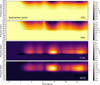 |
Fig. 15 Same as Fig. 14, but for the antistellar point. Mind the different units for the colourbar. |
| In the text | |
|
Fig. 16 Differences in transmission spectra with respect to the pre-fiare state on every time-step during the ~two weeks of flaring according to a FFD, superimposed onto each other in green. The median value of the transit depth on every wavelength is indicated in black. |
| In the text | |
|
Fig. 17 Zonal (τzonal) and meridional (τmerid) advection timescale computed from the GCM outcome of the model planet corresponding to Teff = 800 K with a M dwarf host star, presented in Baeyens et al. (2021). An approximate zonal timescale |
| In the text | |
|
Fig. A.1 Same as Fig. 4, but for CO2, H2O, H, OH, and NH2. We note that the range on the horizontal axis is now extended to lower molar fractions. |
| In the text | |
|
Fig. B.1 Differences in the transmission spectra of the evening and morning limb with respect to the pre-flare state during the flare (lower) and up to Pwind after the flare (upper) for run 2 of Sect. 4.3. |
| In the text | |
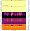 |
Fig. C.1 Same as Fig. 14, but for CO2, H2O, H, OH, and NH2. |
| In the text | |
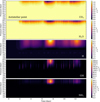 |
Fig. C.2 Same as Fig. 15, but for CO2, H2O, H, OH, and NH2. |
| In the text | |
Current usage metrics show cumulative count of Article Views (full-text article views including HTML views, PDF and ePub downloads, according to the available data) and Abstracts Views on Vision4Press platform.
Data correspond to usage on the plateform after 2015. The current usage metrics is available 48-96 hours after online publication and is updated daily on week days.
Initial download of the metrics may take a while.