| Issue |
A&A
Volume 667, November 2022
|
|
|---|---|---|
| Article Number | A78 | |
| Number of page(s) | 22 | |
| Section | Planets and planetary systems | |
| DOI | https://doi.org/10.1051/0004-6361/202243355 | |
| Published online | 08 November 2022 | |
Spherical harmonic decomposition and interpretation of the shapes of the small Saturnian inner moons★
1
IMCCE, CNRS, Observatoire de Paris, PSL Université, Sorbonne Université,
Université de Lille 1, UMR 8028 du CNRS, 77 Denfert-Rochereau
75014
Paris, France
e-mail: This email address is being protected from spambots. You need JavaScript enabled to view it.
2
Department of Physics and Astronomy, Queen Mary University of London,
Mile End Road,
London
E1 4NS, UK
3
Department of Computer Science, Jinan University,
Guangzhou
510632, PR China
Received:
17
February
2022
Accepted:
24
May
2022
Abstract
Context. The Cassini-Huygens space mission made a series of observations of Saturn’s small satellites during its grand finale stage. These measurements were performed in order to study the shape, geology, and surface composition of the small satellites as well as to study the impact of the environment, in particular the rings, on these small bodies.
Aims. The purpose of this study is to focus on the shape analysis of the small Saturnian satellites in order to describe their global figure and large-scale topography, as well as to deduce fundamental quantities, gravity field, and amplitude of the diurnal libration by assuming that the bodies are homogeneous.
Methods. We used two approaches in this study. On the one hand, we directly exploited the Cassini images of the small satellites by performing limb measurements and deducing a confidence interval on the shape measurements. On the other hand, we used previously published shape models which combine limb measurements and control points. These shape models were then decomposed and described in spherical harmonics.
Results. We found that the shape of the small satellites can be described with a confidence interval between 50 and 150 m. The low degree in spherical harmonics (degree 2) indicated that Telesto, Pandora, Pan, Janus, and Helene have a degree 2 shape close to the Omega sequence, which was defined recently, where the potential is constant along a meridian perpendicular to the longest axis. The degree 2 shape of Epimetheus, on the other hand, is close to the Roche sequence. In contrast, Prometheus, Calypso, and Atlas are in the Low-Brown region. The root mean square spectrum and spherical harmonic maps then allowed us to describe the topography of the satellites, and in particular to highlight equatorial ridges for some satellites including Daphnis. Finally, our estimates of the libration amplitude in the homogeneous case provide values in agreement with previously published librational measurements for Epimetheus while highlighting the proximity of the resonance for Epimetheus, Pandora, and Prometheus.
Conclusions. The high resolution images of the internal satellites have allowed us to describe the geology and the geophysics of these bodies. Future comparison of these amplitudes with new librational measurements deduced, for example, by the astrometric method, will allow us to obtain information on the internal structure of these bodies. Similar studies could be carried out on the internal satellites of Jupiter using images from the Europa Clipper (NASA) or JUICE (ESA) missions.
Key words: planets and satellites: fundamental parameters / planets and satellites: surfaces
Tables A.1–A.10 are only available in electronic form at the CDS via anonymous ftp to cdsarc.cds.unistra.fr (130.79.128.5) or via https://cdsarc.cds.unistra.fr/viz-bin/cat/J/A+A/667/A78
During the period of June-August 2020.
© N. Rambaux et al. 2022
 Open Access article, published by EDP Sciences, under the terms of the Creative Commons Attribution License (https://creativecommons.org/licenses/by/4.0), which permits unrestricted use, distribution, and reproduction in any medium, provided the original work is properly cited.
This article is published in open access under the Subscribe-to-Open model. This email address is being protected from spambots. You need JavaScript enabled to view it. to support open access publication.
1 Introduction
NASA’s Cassini-Huygens space mission explored the Saturn system from 2004 to 2017 and revealed the richness and diversity of Saturn’s satellites (Porco et al. 2007; Buratti et al. 2019). In particular, two families of satellites are classified according to their average radius: the satellites whose average radius R is greater than 100 km and the smaller satellites (R ≤ 100 km) often characterised as inner or small satellites. These satellites have irregular shapes and two mechanisms are proposed to explain them. These satellites either form from the rings (Charnoz et al. 2007; Porco et al. 2007) and their shape is acquired by the accretion of material from an initial core (Charnoz et al. 2007; Quillen et al. 2021) or, alternatively, they grow as a result of slow collisions (Leleu et al. 2018). These two scenarios differ by the size of the interacting bodies and would lead to a different distribution of mass and ridge surface morphologies (Quillen et al. 2021). An understanding of the formation of Saturn’s small satellites would allow for a better understanding of the general formation of giant planet satellites.
The small satellites of Saturn have been observed by the Cassini Narrow Angle Camera (NAC; Porco et al. 2004), and the series of papers by Porco et al. (2007); Thomas (2010); Thomas et al. (2013) and Thomas & Helfenstein (2020) presents the observations and descriptions on the topography, morphology, and geology of the surface of the small satellites. The measurements were used to derive digital terrain models with a representation in the tessellated plate model where the precision is given to about a hundred metres to a kilometre (Porco et al. 2007; Thomas 2010; Thomas et al. 2013; Thomas & Helfenstein 2020). In the family of these small satellites, we can distinguish – in increasing order of distance from Saturn – the following: the A-ring satellites Pan, Daphnis, and Atlas; the F-ring satellites Prometheus and Pandora; the co-orbitals Epimetheus and Janus; the embedded satellites Méthone, Anthe, and Pallene; the co-orbitals of Tethys, including Telesto and Calypso; and finally the co-orbitals of Dione, including Polydeuces and Helene. This paper deals with the satellites where a shape model is now available (Thomas & Helfenstein 2020) and it places special emphasis on Atlas, Prometheus, Pandora, Epimetheus, and Janus where the librational measurements are either accessible or actively sought (Tiscareno et al. 2009; Lainey et al. 2019).
The aim of this paper is to describe the topography of the small satellites from a spherical harmonic (SH) decomposition. This description, when compared to the shape model, allows us to distinguish large spatial structures related to the equilibrium figures (rotation and tides) from the smaller local structures (i.e. ridges) that arise due to endogenous or exogenous processes (e.g. Nimmo et al. 2011; Roberts et al. 2021). In addition, the SH decomposition can allow the extraction of the global shape of the body independently of the cratering surface that induces high degree terms. The SH decomposition acts as a low pass filter, as shown in the case of Phoebe (Rambaux & Castillo-Rogez 2020). In addition, the SH decomposition is useful to derive geophysical and dynamical quantities such as moments of inertia, Stokes coefficients of the gravity field, and libration amplitudes and the secular variation of the periapsis node of the orbits (Lainey et al. 2019), with some additional assumptions on the distribution of mass inside the body. In this paper, we assume that the interior is homogeneous. It would be useful to compare these models in a next step, with astrometrical observations of these satellites and the method can be used as a framework for future missions around giant planets.
This paper is divided into four parts. Section 2 describes the data and the shape model. Then, in Sect. 3, the spherical harmonic decomposition is presented and Sect. 4 presents the topographic surface coefficients derived from the SH decomposition. The last section discusses the interpretation of the data for the small satellites.
2 Observations and shape model data
2.1 Limb profiles
The Cassini-Huygens space mission recorded a large number of images of Saturn’s satellites. In this study, we focus on the small satellites, particularly Atlas, Pandora, Prometheus, Janus, and Epimetheus, whose astrometry has allowed us to constrain their orbital motion and to search for signatures of their librational motion (Lainey et al. 2019). The images of Saturn satellites that were used can be found at the Ring-Moon Systems Node of NASA’s Planetary Data Science, while we used the Caviar software to perform limb measurements. The Caviar software has been developed jointly by Queen Mary University of London and the Institut de Mécanique Céleste et Calcul des Éphémérides (IMCCE; Cooper et al. 2018). This software is dedicated to high accuracy astrometry on images from the Cassini-Huygens mission. The description of the shape models in spherical harmonics that we developed here can be used to improve the satellite astrometry analysis.
The limb measurements are used to study the global shape of bodies (Tajeddine et al. 2017; Thomas & Helfenstein 2020, and references therein), to infer the mean thickness of the elastic layer of some satellites (lithosphere; Nimmo et al. 2011), and also to improve the astrometric accuracy of satellites (Tajeddine et al. 2013; Cooper et al. 2014; Tajeddine et al. 2015). The limb measurement method consists of determining the edge of the satellite illuminated by the Sun or by Saturn, as seen by the Cassini Imaging Science Subsystem (ISS) Narrow-Angle Camera (NAC; see Porco et al. 2004). NASA SPICE routines have been used to reconstruct the geometry and a final translation has been applied in order to correctly centre the computed shape to the observed one. Figure 1 shows a selection of images from the Cassini ISS-NAC with the limb measurement in red and the shape model used and described below in green. This figure demonstrates the generally good agreement between the observed and computed limbs, with a rough agreement to within around a hundred metres.
2.2 Shape model data
Shape models of Saturn’s satellites have been developed over the past several years by Porco et al. (2007), Thomas (2010), Thomas et al. (2013) and recently by Thomas & Helfenstein (2020). These models are based on optical data from the Cassini ISS (see Porco et al. 2004; Thomas & Helfenstein 2020) and more particularly on two data sets: control point networks processed by stereophotogrammetry, and limb measurements which directly provide the satellite’s contours (e.g. Simonelli et al. 1993; Thomas 1993; Thomas et al. 2013). Finally, Thomas & Helfenstein (2020) provided the topography of satellites according to a shape model consisting of a longitude-latitude grid of 2° × 2°. Table 1 compares the models and provides information on the uncertainty of the representation and mean radius, taken from Thomas & Helfenstein (2020).
3 Spherical harmonic approach
The shape models provide the coordinates of points at the surface of the body. As in Rambaux & Castillo-Rogez (2020), we computed the surface coefficients An,m, Bn,m of degree n and order m corresponding to the coefficients of the spherical harmonic decomposition
 (1)
(1)
where r is the radius, λ is the longitude, φ is the latitude, and Pn,m are the un-normalised associated Legendre polynomial of degree n and order m.
The satellite’s SH coefficients and associated uncertainties were determined through two different fits. The first fit used, directly, the shape model provided by Thomas & Helfenstein (2020) as reference points whereas the second one used the limb measurements described in Sect. 2.
In the first approach, we associated an a priori error to each surface point of the shape model equal to the maximum value of the precision provided by Thomas & Helfenstein (2020) and listed in Table 1. Then, the final result of the SH was computed in two iterations. First, all SH coefficients were computed by a least square method up to degree 30. The uncertainties associated with each coefficient were computed by using the covariance matrix. Then we removed from the list all coefficients whose absolute value is smaller than the formal uncertainty. A second iteration, by the least-square method, was performed on the new list of coefficients. We uploaded on CDS website Tables A.1–A.10 of SH coefficients for each body to degree 14, as this is determined below. In this approach, the degree 1 terms are set to zero, which is equivalent to assuming that the origin of the reference frame coincides with the centre of mass.
The Tables of the SH solutions A.1–A.10 (available at the CDS) contain the formal uncertainties derived from the covariance matrix. These uncertainties are much smaller than the a priori uncertainty provided by the shape model (Table 1). This underestimation is due to the fact that the shape model contains a large number of points (13 497 points) related to the coverage steps of 2° by 2°. Such uncertainty is clearly too optimistic because, firstly, fixing the same a priori uncertainty to all points of the grid is too optimistic (some gaps should exist in the observational data set) and, secondly, the value of the formal uncertainties depends on the number of points and in this case there is an arbitrarily large number of points.
To solve the problem of the underestimated uncertainties, we applied the second method consisting of fitting the SH coefficients directly to the limb measurements deduced from Caviar (see Sect. 2). Figure 2 presents the spatial distribution of the limbs for the five selected bodies. These are well distributed on the surface even if not perfectly homogeneous. Then, we fitted the degree 5 SH coefficients to limb profiles by a least-square method. For higher degrees, the process does not converge. This prevents this approach from obtaining a robust determination of the SH coefficients because for irregular satellites it is necessary to go up to degree 14 (see the following paragraph and Fig. 4). However, the covariance matrix provides the uncertainty for degree 2 terms (A20 and A22), which was the objective of this part of the work. Table 2 presents the 3-σ uncertainty for the five satellites. The uncertainties are around a hundred metres, which is consistent with the raw estimation made directly from the images. For the following part of the work, we use these uncertainties.
In order to determine the truncation level required for the fit of the shape model, the limb measurements are used. The objective is to minimise a cost function (χ2) that reflects the amount of information contained in each image. For each satellite, the cost function required the computation of the residuals  for each i image. The index j is for the point of the limb. The O is the observed limb and C is the computed limb based on the SH fitted to the shape model at various maximum degrees. The
  represents the average value O–C for each image. The standard deviation for each image is then σi
 (2)
(2)
Ni is the number of points of the limb for the image i, and the final χ2 is normalised for the set of N images and limb profiles:
![Mathematical equation: ${\chi ^2} = {1 \over {\sum\nolimits_{i = 1}^N {{N_i}} }}\sum\limits_{i = 1}^N {\left[ {\sum\limits_{j = 1}^{{N_i}} {{{\left( {{{{\rm{OC}}_j^i} \over {{\sigma _i}}}} \right)}^2}} } \right]}$](/articles/aa/full_html/2022/11/aa43355-22/aa43355-22-eq5.png) (3)
(3)
The σi values are constant for each case and they are equal to the case where the shape was developed up to degree 20. Another choice could be to keep degree 30 as in our first iteration (see discussion above). However, many coefficients between degrees 20 and 30 are not valid and the choice of degree 20 allows the calculations to be optimised. Figure 3 shows that χ2 converges as a function of the degree to a constant value around degree 14 for all satellites. This behaviour indicates that after this degree, the shape model does not improve the residuals and thus there is no new information. This limits the highest degree. This means that we can use the truncated shape model at degree 14.
Nimmo et al. (2012) emphasise the importance of taking high degrees into account when determining low degrees. Figure 4 and Appendices B.1–B.4 present the estimation of the degree 2 coefficients (A0,0, A2,0, A2,2, and A2,1) for the five selected satellites as a function of the maximum degree. We note that from degree 10, the values of A0,0, A2,0 vary by less than 0.01%, A2,2 varies by less than 0.1%, and A2,1 by less than 3%, confirming the importance of including high-degree coefficients in the fit for irregular satellites.
Section 4.3 describes the gravity field of the internal satellites and the formula from Eq. (10) presents the definition of the Stokes coefficients. These coefficients depend on the mass and reference radius which can be the equatorial radius as in the case of the Earth (Chambat et al. 2010) or a mean radius (Park et al. 2016). Here we use the reference radius of the mean ellipsoid and the associated mass from Thomas & Helfenstein (2020). This choice makes it possible to preserve the average density proposed and described in Thomas & Helfenstein (2020).
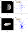 |
Fig. 1 Limb measurements for Atlas (Ia) and Prometheus (IIa). The background is an image coming from ISS (N1560303820 for Atlas and N1640506063 for Prometheus) and the yellow points represent the observed limb deduced from Caviar software and the red points are the shape model deduced from the SH analysis. The left panels (Ib) and (IIb) represent the residues between the observed limb and shape model expressed in kilometers. In the label, we note the root mean square (rms), the standard deviation σ and the scaling factor R. |
Characteristics of inner small satellites of Saturn.
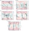 |
Fig. 2 Limbs profiles and Spherical Harmonics mappings for Atlas, Epimetheus, Janus, Pandora, Prometheus. |
Derived confidence interval for A20 and A22 of the five selected satellites.
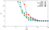 |
Fig. 3 Variation of χ2 as a function of the degree used to describe the shape. |
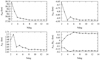 |
Fig. 4 Variation of the degree 2 surface coefficients as function of the degree maximum used in the determination for Epimetheus. |
4 Results and applications
4.1 Spherical harmonic solutions
We applied our methods to all small satellites. The maps shown in Figs. A.1 to A.10 present the topography as a function of the spherical harmonics. Maps (a) represent the topography between degree 0 and 2, (b) degree 0 to 3, (c) degree 3, (d) degree 4, (e) degree 0 to 14, and (f) degree 3 to 14.
Maps A.1 to A.10 (a) describe degrees 0 to 2. Assuming that the satellites form along a Roche ellipsoid and that the low degrees have been slightly modified during the migration of satellites, it should be possible to recover their original shape. To do this, we used the first-order relations between the semi-major axis of the ellipsoid (a1, b1, c1) and the low degrees (cf. Balmino 1994) to extract the semi-major axis ratio of the ellipsoid (b1/a1, c1/a1):
 (4)
(4)
 (5)
(5)
Figure 5 shows, in blue crosses, the semi-major axis ratio determined by the best fit of an ellipsoid to the shape model of Thomas & Helfenstein (2020), our estimation from degree 2 in red, the ideal case of the Roche ellipsoid in green, and the Omega sequence described in Dobrovolskis (2019) in yellow. The general behaviour is to shift the red solution towards the left (smaller b/a ratio), except for Atlas and Helene. For Epimetheus, the red solution is very close to the Roche sequence, whereas Telesto, Pandora, Pan, Helene, and Janus are close to the Omega sequence. Prometheus and Calypso are strongly displaced towards a small b/a ratio. Finally, the small satellites of Saturn seem to be distributed in the Roche sequence, Middle-Brown, close to the Omega sequence and Low-Brown families, following the description of ellipsoidal families by Dobrovolskis (2019).
The maps A.1 to A.10 (b-f) describe the surface variations due to higher degrees and highlight certain geological structures. (1) Maps (e) and (f) of Atlas and Pan show the presence of a pronounced equatorial ridge as noted by Thomas & Helfenstein ((2020). The width of the ridge is latitude ±20° for Atlas, which is (3) very elongated. This elongation is characterised by the strong gradient of slope visible in maps (e) and (f) of these satellites. It is important to note that Daphnis and Telesto are also elongated. (4) Helene and Telesto show a very strong high latitude equator offset of +40° and +15°, respectively. Such an offset could be due to a past pole motion (TPW) and a fossil shape for these two bodies. (5) Finally, Janus and Epimetheus do not show a clear pattern for the high degrees. This behaviour could be the result of an important craterisation of their surface as visible in the images of these two satellites.
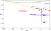 |
Fig. 5 Ratios bT/aT and cT/bT with their uncertainties for the small satellites of Saturn for which DTMs are available (Thomas & Helfenstein 2020). The values in blue represents the best-fit ellipsoids of Thomas & Helfenstein (2020) whereas the red values represent the ellipsoid shape deduced from degrees 2 of our spherical harmonics decomposition. The green curve represents the Roche sequence and yellow line is the Omega sequence defined in Dobrovolskis (2019). |
4.2 Spectrum shape law
This section is dedicated to the computation and interpretation of the topographic power spectrum. Here, we follow the notation and definition of Ermakov et al. (2018) to study the topographical power spectrum RMS  and gravity
  computed for each degree n defined by the following:
 (6)
(6)
 (7)
(7)
This power spectrum has been calculated for several bodies in the Solar System and it generally varies according to a power law close to an exponent of −2 (Vening Meinesz 1951; Ermakov et al. 2018). The recent study by Ermakov et al. (2018) exploits observations of planets, satellites, dwarf planets, and asteroids in the Solar System to suggest a law of the form
 (8)
(8)
where R, ρ, n are the radius, mean density, and degree and A′, α′R, α′ρ, α′n are parameters to fit.
Figures 6 and 7 show the power spectrum RMS for small satellites and the associated uncertainties 1-σ computed with the first approach (so overestimated). Here the fitted parameters derived by Ermakov et al. (2018) are applied. The spectrum and uncertainty lines intersect several times, meaning that the coefficients are not a monotonic function of the degree. Using the shape model, the intersection happens after degree 20 except for Daphnis and Calypso where the intersection is at degree 6 and 8, respectively. In the Daphnis and Calypso cases, it is below the degree 14 value deduced from the χ2 behaviour of our five selected bodies, suggesting its SH coefficients have to be used with caution.
The spectra of Figs. 6 and 7 broadly present a power law where the degree 2 term dominates, largely because of the flattened equatorial bulge and the elongation of the body in the direction of Saturn due to centrifugal and tidal potentials. The spectra of Atlas and Pan show very significant oscillations that are related to the presence of the equatorial ridge similar to the case of asteroids Ryugu and Bennu (Roberts et al. 2021). Daphnis and Calypso also show these very sharp oscillations, but with a smaller amplitude. Some spectra show a relatively large amplitude peak at a specific degree which indicates a prominent topography related to this degree: for example, Epimetheus at degree n = 8, Helene n = 7, Janus n = 5, 8, 14, Pandora n = 10, and Prometheus n = 9, 11. Finally, we see high degree plateaus for some satellites: Telesto (6–7 and 11–12), Helene (11–14), and Pandora (4–6). Such plateaus where the harmonics are no longer correlated with each other could be due to a large crater coverage on the surface of the body, in a similar way to Ryugu (Roberts et al. 2021).
Superimposed on the spectra, we have plotted the best fit of the power law (dashed line) and the interval of solutions proposed by Ermakov et al. (2018). Usually, the best fit power law curves are contained in the interval proposed by Ermakov et al. (2018) with two extreme cases, Atlas and Daphnis, and two cases outside the interval, involving Telesto and Pan. For Atlas, Pan, and slightly for Daphnis and Telesto, this gap is certainly due to the presence of the equatorial ridge. Figure 8 shows the variations of the power law parameters (Eq. (8)) as a function of radius. The distribution of points coincides well with the law proposed by Ermakov et al. (2018) for satellites with a radius greater than 40 km, except for the αn term where the power is in −2.18 and not in −1.88 (Ermakov et al. 2018). On the other hand, for satellites with a radius less than 20 km, no order seems to appear. There are no satellites of intermediate size and therefore the border between these two classes of satellites is very large, about 20 km.
The interpretation of the values of the a parameters remains delicate because several surface mechanisms may be at work. For example, for these small satellites, we can invoke a formation by slow accretion close to the rings, as in Charnoz et al. (2007), Quillen et al. (2021) or mergers during collision as suggested by Leleu et al. (2018). Future studies on this topic would be valuable to link the a values and formation models.
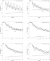 |
Fig. 6 RMS spectrum topography for small satellites of Saturn. The black curve with points represents the spectrum, the solid-black curve is the uncertainty deduced from the least-square fit of the spherical harmonics to the shape models. The dashed-black curve corresponds to the fit of the Vening Meinez-Ermakov laws with the values of the parameters (A, αR, αρ, αn) for all satellites. The gray filled area give the range of values provided in Ermakov et al. (2018). |
4.3 Homogeneous gravity coefficients and moments of inertia
This section discusses the estimation of the Stokes coefficients for an irregular homogeneous body. The objective is to provide reference values where any significant deviations in future observations would be interpreted as a signature of body heterogeneity. As already noted in previous studies, in the case of an irregular body, there is no direct – or simple – transformation between surface coefficients and Stokes coefficients of the gravity filed at a specific degree (e.g. Balmino 1994). It is therefore necessary to introduce surface coefficients of high degree to estimate the Stokes coefficients. In our case, the Stokes coefficients were computed from the moments of inertia, whose expressions are
 (9)
(9)
and the C20 and C22 are
 (10)
(10)
In order to make a link with the previous studies, we use masses and radii, as provided by Thomas & Helfenstein (2020) in their Tables 1 and 2, as references.
Here, we focus only on Atlas, Epimetheus, Janus, Pandora, and Prometheus, whose librations have been previously investigated (Tiscareno et al. 2009; Lainey et al. 2019). In order to obtain the range of possible values of C20 and C22 Stokes coefficients, we included the 3 − σ uncertainty of the surface coefficient deduced in Sect. 3 in our computation. To solve the integrals, Eq. (9) and then C20 and C22, we expanded the surface up to degree 14 and varied surface harmonics coefficients in error bars inside the 3 − σ uncertainty. We ran 500 computations and built the corresponding histogram and then deduced the mean value and standard deviation by fitting a Gaussian curve. The values are reported in Table 3 with the values from Lainey et al. (2019) and the nominal values computed with no variation of the surface coefficients.
The differences between our estimation and the estimation of Lainey et al. (2019) show the effect of using the full shape of the body. For the C20 of Atlas, we note a large difference (10%) between the nominal and mean value. This difference comes from the fact that during the random process, some solutions do not conserve the order of A/MR2 < B/MR2 < C/MR2, leading to an unphysical solution. These solutions are rejected and the resulting mean value of the Stokes coefficient are shifted with respect to the nominal value.
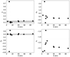 |
Fig. 8 Variation of the parameters A, αR, αρ, and αn for small satellites as function of the radius. The gray filled area/lines represent the values determined in Ermakov et al. (2018). |
Estimation of the degree 2 gravity coefficients C20 and C22 of the five inner small satellites selected.
4.4 Librational amplitude for homogeneous case
The amplitude of the forced libration for the homogeneous case was determined for the following five satellites: Atlas, Epimetheus, Janus, Pandora, and Prometheus. We distinguished the calculation of libration in longitude for the three satellites Atlas, Pandora, and Prometheus, and for the two co-orbitals satellites Janus and Epimetheus which are in horseshoe orbits. In all cases, we assumed that the satellites are in synchronous rotation such as most of the satellites in our Solar System (e.g. Rambaux & Castillo-Rogez 2013) and that the obliquity is negligible. The rotational motion has librations which are oscillations superimposed on the mean rotational motion (e.g. Rambaux 2014).
The approach used to calculate the libration of Atlas, Pandora, and Prometheus follows the classical one (e.g. Rambaux et al. 2010, 2012). In the present work, we have focussed on diurnal physical librations that are expected to be dominant if there is no resonance between the free libration period and an orbital period. As Atlas, Pandora, and Prometheus are very close to Saturn (at [2–2.5] radii from Saturn), we explicitly took the effect of Saturn’s flattening into account in the calculation of the proper mode following Rambaux et al. (2012):
 (11)
(11)
where n is the mean motion of the satellite,  is the triaxaility, J2 is the gravitational coefficient of Saturn, Rp is the Saturn’s radius, and a is the semi-major axis of Saturn-Satellite. We subsequently calculated the amplitude of the first-order libration for the three bodies, following the small libration angle τ and low-eccentricity e approximations:
 (12)
(12)
If the free frequency ω0 is small with respect to n, then the amplitude of the libration is at first order A = 6eγ. On the other hand, when ω0 is of the order of n, the amplitude increases because of the proximity with a resonance and the small angle approximation is no longer valid as shown in Fig. 9 computed for each satellite. It is interesting to note that the amplitudes of Epimetheus, Pandora, and – to lesser extent – Prometheus are particularly sensitive to the value of γ due to the proximity with the resonance. Such large amplitudes could lead to grooves at the surface of these bodies (Thomas & Helfenstein 2020).
The small satellite Epimetheus is in 1:1 orbital resonance with Janus, implying a horseshoe-shape orbit. This peculiar orbit presents a swap in semi-major axis of a few tens of kilometres that perturbs the librational motion. In order to describe the effect of the swap on the librational motion, Robutel et al. (2011) developed a quasi-periodic librational model where the librations A are decomposed as
![Mathematical equation: $\matrix{A \hfill & = \hfill & {\sum\limits_{1 \le q \le N} {{\beta _{\rm{q}}}\sin \left( {qvt + {\varphi _{\rm{q}}}} \right) + {{2e{{\bar \sigma }^2}{J_0}\left( {{\beta _1}} \right)} \over {\omega _0^2 - {n^2}}}\sin \left( {nt + {\ell _0}} \right)} } \hfill \cr{} \hfill & {} \hfill & { + 2e\omega _0^2\sum\limits_{{\rm{p}} \ge {\rm{1}}} {{J_{\rm{p}}}\left( {{\beta _1}} \right)} \left[ {{{\sin \left( {\left( {n + pv} \right)t + p{\varphi _1} + {\ell _0}} \right)} \over {\omega _0^2 - {{\left( {n + pv} \right)}^2}}}} \right.} \hfill \cr{} \hfill & {} \hfill & {\left. { + {{\left( { - 1} \right)}^p}{{\sin \left( {\left( {n + pv} \right)t - p{\varphi _1} + {\ell _0}} \right)} \over {\omega _0^2 - {{\left( {n - pv} \right)}^2}}}} \right].} \hfill \cr}$](/articles/aa/full_html/2022/11/aa43355-22/aa43355-22-eq18.png) (13)
(13)
The first sum represents the long-period term directly related to the swap motion. In this sum, βq are the coefficients of the quasi-periodic series from the variations of the mean longitude, v is the frequency of the swap, and φq is its phase. The short period librations are described by the second and third terms. Their frequencies are of the order of n, the geometrical mean motion, with harmonics in v. The constants Jp are the Bessel functions.
To estimate the libration amplitude, we used the triaxility extracted from the Monte Carlo runs calculated in the previous step, Sect. 4.3. As the relationship between the libration amplitude and triaxility is not linear, we constrained the uncertainty by computing the proportion of the ±0.33 quantile from the median value. Table 4 presents the resulting amplitude of the theoretical librations assuming that each body is homogeneous. The first line “La19 Theo” corresponds to the theoretical estimates of Lainey et al. (2019) where the moments of inertia were computed based on the ellipsoid assumption. Then, the line “La19 Obs” shows the astrometric results (Lainey et al. 2019) and “Ti09” presents the results for Epimetheus and Janus from Cassini s stereoscopic measurements (Tiscareno et al. 2009). The next four rows show our amplitude of librations where the nominal refers to the solution without a variation in the surface coefficients and solutions coming from our Monte Carlo estimation of uncertainties expressed here in quantiles. We also distinguished solutions without and with Saturnian J2. We note that our estimations for Epimetheus and Janus are fully consistent with the observations of Tiscareno et al. (2009), while confirming the disagreement obtained by Lainey et al. (2019). In this latter paper – which used ellipsoidal shapes for both astrometric reduction and libration amplitude calculation – the error bars were not 1 -sigma, but something way more conservative. The correction of the free frequency with the Saturnian J2 results in an increase in the librational amplitude of Epimetheus and Pandora. This effect is due to the proximity with the resonance as illustrated in Fig. 9. The amplitude of libration for Epimetheus is also closer to the observed value determined by Tiscareno et al. (2009). In the present paper, we establish the magnitude orders of Stokes coefficients and libration amplitude by taking the full shape models into account and by estimating thoroughly the uncertainties related to the observations.
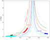 |
Fig. 9 Amplitude of librations A as function of triaxility γ for the eccentricities corresponding to small satellites: Atlas (cyan), Epimetheus (pink), Janus (green), Pandora (red), Prometheus (blue). The eccentricity values are indicated in the figure. |
Libration amplitude of the five inner small satellites selected.
5 Conclusion
This paper is dedicated to the study of the surfaces of the small Saturnian satellites using a spherical harmonic decomposition. The decomposition is based on a shape model provided by Thomas & Helfenstein (2020) and the uncertainties are directly deduced from the limb measurements obtained from images taken using the ISS camera of the Cassini-Huygens mission. We deduced the degree 2 global shape of the satellites and have shown that some satellites have shapes close to the Roche ellipsoids or the Omega sequence according to the classification of Dobrovolskis (2019). Following this, an analysis of the RMS spectrum and the SH maps allowed us to describe and confirm the presence of ridges, longitudinal structures, and strong gradient slopes. The analysis of the RMS spectrum highlights the minimum radius, 20–40 km, from which the bodies follow the Vening-Meinez law (Ermakov et al. 2018). Finally, we have estimated the fundamental quantities such as the gravity field at degree 2 and libration amplitude for a selection of five satellites for which astrometric or stereo-photogrammetric measurements are available today. We found that Epimetheus, Pandora, and Prometheus present large amplitudes due to their proximity with the resonance between free and forced librations. These large amplitudes could add constraints on the formation of grooves at the surface of these bodies (Thomas & Helfenstein 2020). These theoretical values of geodetical quantities deduced in the homogeneous case could be compared to the Cassini ISS measurements to provide information on the internal structure of these satellites, which are precursors of the larger icy satellites. The determination of the moments of inertia can provide information on the origin and morphological processes of these bodies. Indeed, at present, two scenarios are proposed for the morphology: the ornamental accretion (Charnoz et al. 2007; Quillen et al. 2021) for Atlas, Pan, and Daphnis, and a slow merger collision (Leleu et al. 2018) for all of them. In the first case, a seed composed of silicate is surrounded by ice coming from the rings by a heterogeneous accretion process or, if all silicate were depleted, the seed could be composed of ice (Charnoz et al. 2007, 2011). In the second case, the slow collision between the two progenitors would lead to a macroscopic homogenisation by mixing the two materials. These different internal structure scenarios can be tested by measuring the librations and gravity coefficients as proposed in the case of Phobos (Rambaux et al. 2012; Le Maistre et al. 2019). Finally, this work can be applied to the satellites close to Jupiter that will be observed by the Europa Clipper (NASA) and JUICE (ESA) missions.
Acknowledgements
We thank the Ring-Moon Systems Node of NASA’s Planetary Data Science to collect and open data science. We thank Peter Thomas and Sebastien Charnoz for fruitful discussions and the referee for his careful reading and helpful suggestions.
Appendix A SH maps
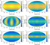 |
Fig. A.1 Topographic mapping of satellite Atlas. The figure (a) represents the distribution for degrees 0 to 2, (b) for degrees 0 to 3, (c) the degree 3, (d) the degree 4, (e) from degree 0 to 14 and (f) from degree 3 to 14. |
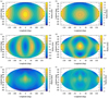 |
Fig. A.2 Topographic mapping of satellite Calypso. The figure (a) represents the distribution for degrees 0 to 2, (b) for degrees 0 to 3, (c) the degree 3, (d) the degree 4, (e) from degree 0 to 8 and (f) from degree 3 to 8. |
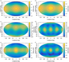 |
Fig. A.3 Topographic mapping of satellite Daphnis. The figure (a) represents the distribution for degrees 0 to 2, (b) for degrees 0 to 3, (c) the degree 3, (d) the degree 4, (e) from degree 0 to 6 and (f) from degree 3 to 6. |
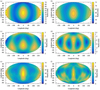 |
Fig. A.4 Topographic mapping of satellite Epimetheus. The figure (a) represents the distribution for degrees 0 to 2, (b) for degrees 0 to 3, (c) the degree 3, (d) the degree 4, (e) from degree 0 to 14 and (f) from degree 3 to 14. |
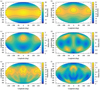 |
Fig. A.5 Topographic mapping of satellite Helene. The figure (a) represents the distribution for degrees 0 to 2, (b) for degrees 0 to 3, (c) the degree 3, (d) the degree 4, (e) from degree 0 to 14 and (f) from degree 3 to 14. |
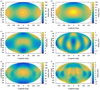 |
Fig. A.6 Topographic mapping of satellite Janus. The figure (a) represents the distribution for degrees 0 to 2, (b) for degrees 0 to 3, (c) the degree 3, (d) the degree 4, (e) from degree 0 to 14 and (f) from degree 3 to 14. |
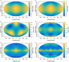 |
Fig. A.7 Topographic mapping of satellite Pan. The figure (a) represents the distribution for degrees 0 to 2, (b) for degrees 0 to 3, (c) the degree 3, (d) the degree 4, (e) from degree 0 to 14 and (f) from degree 3 to 14. |
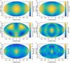 |
Fig. A.8 Topographic mapping of satellite Pandora. The figure (a) represents the distribution for degrees 0 to 2, (b) for degrees 0 to 3, (c) the degree 3, (d) the degree 4, (e) from degree 0 to 14 and (f) from degree 3 to 14. |
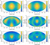 |
Fig. A.9 Topographic mapping of satellite Prometheus. The figure (a) represents the distribution for degrees 0 to 2, (b) for degrees 0 to 3, (c) the degree 3, (d) the degree 4, (e) from degree 0 to 14 and (f) from degree 3 to 14. |
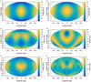 |
Fig. A.10 Topographic mapping of satellite Telesto. The figure (a) represents the distribution for degrees 0 to 2, (b) for degrees 0 to 3, (c) the degree 3, (d) the degree 4, (e) from degree 0 to 14 and (f) from degree 3 to 14. |
Appendix B Influence of low degree
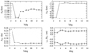 |
Fig. B.1 Variation of the degree 2 surface coefficients as function of the degree maximum used in the determination for Atlas. |
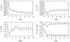 |
Fig. B.2 Variation of the degree 2 surface coefficients as function of the degree maximum used in the determination for Janus, Pandora, Prometeheus. |
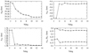 |
Fig. B.3 Variation of the degree 2 surface coefficients as function of the degree maximum used in the determination for Pandora. |
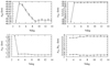 |
Fig. B.4 Variation of the degree 2 surface coefficients as function of the degree maximum used in the determination for Prometeheus. |
References
- Balmino, G. 1994, Celest. Mech. Dyn. Astron., 60, 331 [NASA ADS] [CrossRef] [Google Scholar]
- Buratti, B. J., Thomas, P. C., Roussos, E., et al. 2019, Science, 364, 6445 [CrossRef] [Google Scholar]
- Chambat, F., Ricard, Y., & Valette, B. 2010, Geophys. J. Int., 183, 727 [NASA ADS] [CrossRef] [Google Scholar]
- Charnoz, S., Brahic, A., Thomas, P. C., & Porco, C. C. 2007, Science, 318, 1622 [NASA ADS] [CrossRef] [Google Scholar]
- Charnoz, S., Crida, A., Castillo-Rogez, J. C., et al. 2011, Icarus, 216, 535 [NASA ADS] [CrossRef] [Google Scholar]
- Cooper, N. J., Murray, C. D., Lainey, V., et al. 2014, A&A, 572, A43 [NASA ADS] [CrossRef] [EDP Sciences] [Google Scholar]
- Cooper, N. J., Lainey, V., Meunier, L. E., et al. 2018, A&A, 610, A2 [NASA ADS] [CrossRef] [EDP Sciences] [Google Scholar]
- Dobrovolskis, A. R. 2019, Icarus, 321, 891 [NASA ADS] [CrossRef] [Google Scholar]
- Ermakov, A. I., Park, R. S., & Bills, B. G. 2018, J. Geophys. Res. (Planets), 123, 2038 [NASA ADS] [CrossRef] [Google Scholar]
- Lainey, V., Noyelles, B., Cooper, N., et al. 2019, Icarus, 326, 48 [Google Scholar]
- Le Maistre, S., Rivoldini, A., & Rosenblatt, P. 2019, Icarus, 321, 272 [NASA ADS] [CrossRef] [Google Scholar]
- Leleu, A., Jutzi, M., & Rubin, M. 2018, Nat. Astron., 2, 555 [NASA ADS] [CrossRef] [Google Scholar]
- Nimmo, F., Bills, B. G., & Thomas, P. C. 2011, J. Geophys. Res. (Planets), 116, E11001 [CrossRef] [Google Scholar]
- Nimmo, F., Faul, U. H., & Garnero, E. J. 2012, J. Geophys. Res. (Planets), 117, 9005 [Google Scholar]
- Park, R. S., Konopliv, A. S., Bills, B. G., et al. 2016, Nature, 537, 515 [NASA ADS] [CrossRef] [Google Scholar]
- Porco, C. C., West, R. A., Squyres, S., et al. 2004, Space Sci. Rev., 115, 363 [NASA ADS] [CrossRef] [Google Scholar]
- Porco, C. C., Thomas, P. C., Weiss, J. W., & Richardson, D. C. 2007, Science, 318, 1602 [NASA ADS] [CrossRef] [Google Scholar]
- Quillen, A. C., Zaidouni, F., Nakajima, M., & Wright, E. 2021, Icarus, 357, 114260 [NASA ADS] [CrossRef] [Google Scholar]
- Rambaux, N. 2014, in Journées 2013 “Systèmes de référence spatio-temporels”, ed. N. Capitaine, 235 [Google Scholar]
- Rambaux, N., & Castillo-Rogez, J. 2013, Tides on Satellites of Giant Planets, eds. J. Souchay, S. Mathis, & T. Tokieda, (Springer-Verlag Berlin Heidelberg), 861, 167 [NASA ADS] [Google Scholar]
- Rambaux, N., & Castillo-Rogez, J. C. 2020, A&A, 643, A10 [NASA ADS] [CrossRef] [EDP Sciences] [Google Scholar]
- Rambaux, N., Castillo-Rogez, J. C., Williams, J. G., & Karatekin, Ö. 2010, Geophys. Res. Lett., 37, 4202 [NASA ADS] [CrossRef] [Google Scholar]
- Rambaux, N., Castillo-Rogez, J. C., Le Maistre, S., & Rosenblatt, P. 2012, A&A, 548, A14 [NASA ADS] [CrossRef] [EDP Sciences] [Google Scholar]
- Roberts, J. H., Barnouin, O. S., Daly, M. G., et al. 2021, Planet. Space Sci., 204, 105268 [NASA ADS] [CrossRef] [Google Scholar]
- Robutel, P., Rambaux, N., & Castillo-Rogez, J. 2011, Icarus, 211, 758 [NASA ADS] [CrossRef] [Google Scholar]
- Simonelli, D. P., Thomas, P. C., Carcich, B. T., & Veverka, J. 1993, Icarus, 103, 49 [NASA ADS] [CrossRef] [Google Scholar]
- Tajeddine, R., Cooper, N. J., Lainey, V., Charnoz, S., & Murray, C. D. 2013, A&A, 551, A129 [NASA ADS] [CrossRef] [EDP Sciences] [Google Scholar]
- Tajeddine, R., Lainey, V., Cooper, N. J., & Murray, C. D. 2015, A&A, 575, A73 [NASA ADS] [CrossRef] [EDP Sciences] [Google Scholar]
- Tajeddine, R., Soderlund, K. M., Thomas, P. C., et al. 2017, Icarus, 295, 46 [NASA ADS] [CrossRef] [Google Scholar]
- Thomas, P. C. 1993, Icarus, 105, 326 [NASA ADS] [CrossRef] [Google Scholar]
- Thomas, P. C. 2010, Icarus, 208, 395 [NASA ADS] [CrossRef] [Google Scholar]
- Thomas, P., & Helfenstein, P. 2020, Icarus, 344, 113355 [NASA ADS] [CrossRef] [Google Scholar]
- Thomas, P. C., Burns, J. A., Hedman, M., et al. 2013, Icarus, 226, 999 [NASA ADS] [CrossRef] [Google Scholar]
- Tiscareno, M. S., Thomas, P. C., & Burns, J. A. 2009, Icarus, 204, 254 [NASA ADS] [CrossRef] [Google Scholar]
- Vening Meinesz, F. A. 1951, in Proceedings Koninklijke Nederlandse Academie van Wetenschappen Series B Physical Sciences, 54 [Google Scholar]
All Tables
Estimation of the degree 2 gravity coefficients C20 and C22 of the five inner small satellites selected.
All Figures
|
Fig. 1 Limb measurements for Atlas (Ia) and Prometheus (IIa). The background is an image coming from ISS (N1560303820 for Atlas and N1640506063 for Prometheus) and the yellow points represent the observed limb deduced from Caviar software and the red points are the shape model deduced from the SH analysis. The left panels (Ib) and (IIb) represent the residues between the observed limb and shape model expressed in kilometers. In the label, we note the root mean square (rms), the standard deviation σ and the scaling factor R. |
| In the text | |
|
Fig. 2 Limbs profiles and Spherical Harmonics mappings for Atlas, Epimetheus, Janus, Pandora, Prometheus. |
| In the text | |
|
Fig. 3 Variation of χ2 as a function of the degree used to describe the shape. |
| In the text | |
|
Fig. 4 Variation of the degree 2 surface coefficients as function of the degree maximum used in the determination for Epimetheus. |
| In the text | |
|
Fig. 5 Ratios bT/aT and cT/bT with their uncertainties for the small satellites of Saturn for which DTMs are available (Thomas & Helfenstein 2020). The values in blue represents the best-fit ellipsoids of Thomas & Helfenstein (2020) whereas the red values represent the ellipsoid shape deduced from degrees 2 of our spherical harmonics decomposition. The green curve represents the Roche sequence and yellow line is the Omega sequence defined in Dobrovolskis (2019). |
| In the text | |
|
Fig. 6 RMS spectrum topography for small satellites of Saturn. The black curve with points represents the spectrum, the solid-black curve is the uncertainty deduced from the least-square fit of the spherical harmonics to the shape models. The dashed-black curve corresponds to the fit of the Vening Meinez-Ermakov laws with the values of the parameters (A, αR, αρ, αn) for all satellites. The gray filled area give the range of values provided in Ermakov et al. (2018). |
| In the text | |
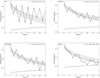 |
Fig. 7 Same as in Fig. 6. |
| In the text | |
|
Fig. 8 Variation of the parameters A, αR, αρ, and αn for small satellites as function of the radius. The gray filled area/lines represent the values determined in Ermakov et al. (2018). |
| In the text | |
|
Fig. 9 Amplitude of librations A as function of triaxility γ for the eccentricities corresponding to small satellites: Atlas (cyan), Epimetheus (pink), Janus (green), Pandora (red), Prometheus (blue). The eccentricity values are indicated in the figure. |
| In the text | |
|
Fig. A.1 Topographic mapping of satellite Atlas. The figure (a) represents the distribution for degrees 0 to 2, (b) for degrees 0 to 3, (c) the degree 3, (d) the degree 4, (e) from degree 0 to 14 and (f) from degree 3 to 14. |
| In the text | |
|
Fig. A.2 Topographic mapping of satellite Calypso. The figure (a) represents the distribution for degrees 0 to 2, (b) for degrees 0 to 3, (c) the degree 3, (d) the degree 4, (e) from degree 0 to 8 and (f) from degree 3 to 8. |
| In the text | |
|
Fig. A.3 Topographic mapping of satellite Daphnis. The figure (a) represents the distribution for degrees 0 to 2, (b) for degrees 0 to 3, (c) the degree 3, (d) the degree 4, (e) from degree 0 to 6 and (f) from degree 3 to 6. |
| In the text | |
|
Fig. A.4 Topographic mapping of satellite Epimetheus. The figure (a) represents the distribution for degrees 0 to 2, (b) for degrees 0 to 3, (c) the degree 3, (d) the degree 4, (e) from degree 0 to 14 and (f) from degree 3 to 14. |
| In the text | |
|
Fig. A.5 Topographic mapping of satellite Helene. The figure (a) represents the distribution for degrees 0 to 2, (b) for degrees 0 to 3, (c) the degree 3, (d) the degree 4, (e) from degree 0 to 14 and (f) from degree 3 to 14. |
| In the text | |
|
Fig. A.6 Topographic mapping of satellite Janus. The figure (a) represents the distribution for degrees 0 to 2, (b) for degrees 0 to 3, (c) the degree 3, (d) the degree 4, (e) from degree 0 to 14 and (f) from degree 3 to 14. |
| In the text | |
|
Fig. A.7 Topographic mapping of satellite Pan. The figure (a) represents the distribution for degrees 0 to 2, (b) for degrees 0 to 3, (c) the degree 3, (d) the degree 4, (e) from degree 0 to 14 and (f) from degree 3 to 14. |
| In the text | |
|
Fig. A.8 Topographic mapping of satellite Pandora. The figure (a) represents the distribution for degrees 0 to 2, (b) for degrees 0 to 3, (c) the degree 3, (d) the degree 4, (e) from degree 0 to 14 and (f) from degree 3 to 14. |
| In the text | |
|
Fig. A.9 Topographic mapping of satellite Prometheus. The figure (a) represents the distribution for degrees 0 to 2, (b) for degrees 0 to 3, (c) the degree 3, (d) the degree 4, (e) from degree 0 to 14 and (f) from degree 3 to 14. |
| In the text | |
|
Fig. A.10 Topographic mapping of satellite Telesto. The figure (a) represents the distribution for degrees 0 to 2, (b) for degrees 0 to 3, (c) the degree 3, (d) the degree 4, (e) from degree 0 to 14 and (f) from degree 3 to 14. |
| In the text | |
|
Fig. B.1 Variation of the degree 2 surface coefficients as function of the degree maximum used in the determination for Atlas. |
| In the text | |
|
Fig. B.2 Variation of the degree 2 surface coefficients as function of the degree maximum used in the determination for Janus, Pandora, Prometeheus. |
| In the text | |
|
Fig. B.3 Variation of the degree 2 surface coefficients as function of the degree maximum used in the determination for Pandora. |
| In the text | |
|
Fig. B.4 Variation of the degree 2 surface coefficients as function of the degree maximum used in the determination for Prometeheus. |
| In the text | |
Current usage metrics show cumulative count of Article Views (full-text article views including HTML views, PDF and ePub downloads, according to the available data) and Abstracts Views on Vision4Press platform.
Data correspond to usage on the plateform after 2015. The current usage metrics is available 48-96 hours after online publication and is updated daily on week days.
Initial download of the metrics may take a while.