| Issue |
A&A
Volume 684, April 2024
|
|
|---|---|---|
| Article Number | L3 | |
| Number of page(s) | 5 | |
| Section | Letters to the Editor | |
| DOI | https://doi.org/10.1051/0004-6361/202449639 | |
| Published online | 05 April 2024 | |
Letter to the Editor
Tidal frequency dependence of the Saturnian k2 Love number
1
IMCCE, Observatoire de Paris, PSL Research University, CNRS, Sorbonne Université, Univ. Lille, France
e-mail: This email address is being protected from spambots. You need JavaScript enabled to view it.
2
Canadian Institute for Theoretical Astrophysics, 60 St. George Street, Toronto, ON M5S 3H8, Canada
3
TAPIR, Mailcode 350-17, California Institute of Technology, Pasadena, CA 91125, USA
4
Department of Physics & Astronomy, Queen Mary University of London, Mile End Rd, London E1 4NS, UK
5
Department of Computer Science, Jinan University, Guangzhou 510632, PR China
Received:
16
February
2024
Accepted:
18
March
2024
Abstract
Context. Love numbers describe the fluid and elastic response of a body to the tidal force of another massive object. By quantifying these numbers, we can more accurately model the interiors of the celestial objects concerned.
Aims. We determine Saturn’s degree-2 Love number, k2, at four different tidal forcing frequencies.
Methods. To do this, we used astrometric data from the Cassini spacecraft and a dynamical model of the orbits of Saturn’s moons.
Results. The values obtained for k2 are 0.384 ± 0.015, 0.370 ± 0.023, 0.388 ± 0.006, and 0.376 ± 0.007 (1σ error bar) for the tidal frequencies of Janus–Epimetheus, Mimas, Tethys, and Dione.
Conclusions. We show that these values are compatible with a constant Love number formulation. In addition, we compared the observed values with models of dynamical tides excited in Saturn’s interior, also finding a good agreement. Future increases in the measurement precision of Love numbers will provide new constraints on the internal structure of Saturn.
Key words: astrometry / celestial mechanics / planets and satellites: dynamical evolution and stability / planets and satellites: fundamental parameters / planets and satellites: gaseous planets / planets and satellites: interiors
© The Authors 2024
 Open Access article, published by EDP Sciences, under the terms of the Creative Commons Attribution License (https://creativecommons.org/licenses/by/4.0), which permits unrestricted use, distribution, and reproduction in any medium, provided the original work is properly cited.
This article is published in open access under the Subscribe to Open model. This email address is being protected from spambots. You need JavaScript enabled to view it. to support open access publication.
1. Introduction
Among the most surprising results obtained with the Cassini probe concerning the orbital dynamics of Saturn’s moons was the quantification of tidal effects on Saturn. Using thousands of astrometric data points from the Cassini Imaging Science Subsystem (ISS) Narrow Angle Camera (NAC) images (Porco et al. 2004), Lainey et al. (2012) were able to measure the rapid orbital expansion of the moons. This is characterized by the tidal ratio k2/Q, where k2 is the degree-2 Love number and Q is the quality factor characterizing the dissipation of tidal energy in the planet. Using the motion of the four co-orbital moons of Tethys and Dione, Lainey et al. (2017) were able to independently quantify the two parameters, k2 and Q. In a later work, Lainey et al. (2020) even managed to quantify the quality factor Q at six different frequencies, corresponding to the tidal frequencies associated with Mimas, Enceladus, Tethys, Dione, Rhea, and Titan.
In the present work, we investigated whether it is also possible to quantify Saturn’s k2 Love number at different tidal frequencies. Using all the astrometric data currently available, we show that it can be quantified at four tidal frequencies associated with the action of the moons Janus and Epimetheus (being on a horseshoe orbit, both moons share the same tidal frequency), Mimas, Tethys, and Dione. We then compared the results obtained with the values predicted by modelling the dynamical tidal response of the planet, including its fundamental and gravito-inertial modes and inertial waves.
In Sect. 2 we present the dynamical modeling used, as well as the fitting of the orbital model to astrometric data from the Cassini probe. In Sect. 3 we briefly present how Saturn’s interior was modelled and compare the results obtained from astrometry with our model.
2. Orbital fit
We carried out orbital dynamical modelling and fitting to the observations in a similar way as Lainey et al. (2023, 2024), with the additional improvement of solving for an independent k2 for the frequency of each tide-raising moon. For convenience, we review our method and the relevant equations below, and refer the reader to Lainey et al. (2023, 2024) for further details.
2.1. Dynamical modelling
Using the NOE (Numerical Orbit and Ephemerides) gravitational N-body code (Lainey et al. 2007), we fitted the full equations of motion (see Eq. (1)) to the available astrometric observations (see Sect. 2.2), solving for the initial positions and velocities of: the eight main moons; the four co-orbitals Telesto, Calypso, Helen, and Polydeuces; the five inner moons Atlas, Prometheus, Pandora, Janus, and Epimetheus; and the small moons Methone, Anthe, and Pallene. In addition, global parameters, such as the masses, the Cnp and Snp gravity coefficients, and the Saturnian polar orientation, were simultaneously solved for. Following Lainey et al. (2023), the physical librations of Prometheus, Pandora, Janus, and Epimetheus were also considered. Lastly, the Saturnian Love number associated with each tide-raising moon was solved for, together with a supposedly constant Saturnian Love number, k3.
Our model included (i) gravitational interactions up to degree 2 in the expansion of the gravitational potential of the satellites (Table 2 from Lainey et al. 2019) and degree 10 for Saturn (Iess et al. 2019; ii) gravitational perturbations between all moons; (iii) the solar perturbation (where the masses of the inner planets and the Moon were incorporated into the solar mass) and the Jupiter perturbation based on the DE430 ephemeris; (iv) the precession of Saturn; (v) tidal effects based on the Love numbers k2 and k3, neglecting dissipation; and (vi) relativistic corrections.
Following Lainey et al. (2007), the equation of motion for a satellite Pi can be expressed as
 (1)
(1)
where ri and rj are the position vectors of satellite Pi and a perturbing body, Pj (another satellite, the Sun, or a planet) with mass mj, respectively, the subscript 0 denotes Saturn, and  is associated with the gravity field of body Pl at the position of body Pk (including planetary oblateness). In particular, we have
![Mathematical equation: $$ \begin{aligned} V_{\bar{k}\hat{l}}=\sum _{n=1}^\infty \frac{R^n}{r^{n+1}}\sum _{p=0}^nP_n^p(\sin \phi )[C_{np}\cos p \lambda +S_{np}\sin p \lambda ], \end{aligned} $$](/articles/aa/full_html/2024/04/aa49639-24/aa49639-24-eq3.gif) (2)
(2)
where R, Cnp, and Snp are the radius and gravity field coefficients of the oblate body, Pl, while r, ϕ, and λ are the spherical coordinates of the disturbed object, Pk. Moreover, GR are corrections due to general relativity (Newhall et al. 1983). The  is the force on Pl from the tides it raises on its primary body, and
  is the effect of tides raised by one moon on Saturn acting on another moon. In the absence of tidal dissipation, these last two forces are given by Lainey et al. (2007, 2017):
 (3)
(3)
![Mathematical equation: $$ \begin{aligned}&{\boldsymbol{F}}^T_{ij} = \frac{3k_2Gm_jm_iR^5}{2r^5_i r^5_j}\left[-\frac{5({\boldsymbol{r}}_i\cdot {\boldsymbol{r}}_j)^2{\boldsymbol{r}}_i}{r^2_i}+r^2_j{\boldsymbol{r}}_i+2({\boldsymbol{r}}_i\cdot {\boldsymbol{r}}_j){\boldsymbol{r}}_j\right]. \end{aligned} $$](/articles/aa/full_html/2024/04/aa49639-24/aa49639-24-eq7.gif) (4)
(4)
Here, the k2 Love number is defined as
 (5)
(5)
where δΦnp and Unp are coefficients associated with the angular dependence n, p in the perturbed and perturbing gravitational potentials. We assumed k2 = k20 = k21 = k22. A similar equation can be obtained with the third-order Love number, k3:
![Mathematical equation: $$ \begin{aligned} {\boldsymbol{F}}_{ij}^{T_{k_3}}=&\frac{Gm_jm_ik_3R^7}{2r_i^7r_j^7} \left\{ 5({\boldsymbol{r}_i}\cdot {\boldsymbol{r}_j})\left[3r_j^2-7 \frac{({\boldsymbol{r}_i}\cdot {\boldsymbol{r}}_j)^2}{r_i^2}\right]{\boldsymbol{r}}_i\right.\nonumber \\&\left.+3[5({\boldsymbol{r}_i}\cdot {\boldsymbol{r}}_j)^2-r_i^2r_j^2]{\boldsymbol{r}_j}\right\} . \end{aligned} $$](/articles/aa/full_html/2024/04/aa49639-24/aa49639-24-eq9.gif) (6)
(6)
The physical libration of the moon Pi arises implicitly in the expression of  and
and  in Eq. (1). For more details, the reader can refer to Eqs. (22) and (23) in Lainey et al. (2019).
Our fitting process involved solving the variational equations for an unspecified parameter, cl, of the model to be fitted (e.g. r(t0),dr/dt(t0),Q…; see Lainey 2016 for more details):
![Mathematical equation: $$ \begin{aligned} \frac{\partial }{\partial c_l}\left(\frac{d^2{\boldsymbol{r}}_i}{\mathrm{d}t^2}\right) = \frac{1}{m_i}\left[\sum _j\left(\frac{\partial {\boldsymbol{F}}_i}{\partial {\boldsymbol{r}}_j}\frac{\partial {\boldsymbol{r}}_j}{\partial c_l}+\frac{\partial {\boldsymbol{F}}_i}{\partial \dot{{\boldsymbol{r}}}_j} \frac{\partial \dot{{\boldsymbol{r}}}_j}{\partial c_l}\right)+\frac{\partial {\boldsymbol{F}}_i}{\partial c_l}\right]\cdot \end{aligned} $$](/articles/aa/full_html/2024/04/aa49639-24/aa49639-24-eq12.gif) (7)
(7)
In this expression, Fi is the right-hand side of Eq. (1) multiplied by mi. The partial derivatives of the solutions with respect to the initial positions and velocities of the satellites and the dynamical parameters were then computed via the simultaneous numerical solution of Eqs. (1) and (7), in a Saturn-centred frame with inertial axes based on the International Celestial Reference Frame.
To test the reliability of our fit, we considered extra perturbations. Among other effects, we considered the influence of Mimas’s extended gravity field, the Saturnian nutations from the SAT427 SPICE kernel (Acton 1996), the Saturnian polar orientation determined by French et al. (2017), and the influence of using different Cassini orbit kernels. All these perturbations were found to be negligible within the uncertainty of our measurements.
In summary, all our simulations involved simultaneously solving for the initial state vectors and masses of the moons, the mass and gravity field of Saturn, including zonal harmonics up to order 10, the orientation and precession of Saturn, and the physical librations for Prometheus, Pandora, Janus, and Epimetheus. No constraints were introduced in the fit, except for Saturn’s gravity field at the value estimated by Iess et al. (2019) assuming their published 1σ uncertainty. Last, we included the uncertainty on the tidal frequency dependence of the Saturnian Q parameter in the error bar of our measurements.
2.2. Fitting the data
We used all astrometric data available for the moons (Tajeddine et al. 2013, 2015; Cooper et al. 2014, 2018; Zhang et al. 2021; Lainey et al. 2023, 2024). Our astrometric residuals are given in Tables 1–3. To test the frequency sensitivity of the tidal frequency k2 Love number, we used a two-step method. In the first step we solved for a constant k2 and k3 and obtained k2 = 0.384 ± 0.004 and k3 = 0.005 ± 0.111 (1σ error bar). In the second step, we solved for the k2 at all of the moons’ frequencies. Only four tidal frequencies could be fairly well constrained: the tides associated with Janus and Epimetheus, Mimas, Tethys, and Dione. In this second approach, we eventually used the constant k3 and k2 solution from the first approach for the other tidal frequencies.
Mean (ν) and standard deviation (σ) of the sample and line residuals (in pixels) for each satellite (Cassini-ISS data).
Mean (ν) and standard deviation (σ) of the sample and line residuals (in pixels) for each satellite (Cassini-ISS data).
Statistics of the ISS-NAC astrometric residuals computed in km.
From our second approach (using a non-constant k2 Love number), we find that the Love number values obtained for the Janus–Epimetheus, Tethys, and Dione frequencies were obtained from cross tidal–tidal effects acting on the co-orbital moons. In other words, the tidal bulge of Saturn raised by one moon was measured through its effect on co-orbital moons in the exact same manner as described in Lainey et al. (2017). On the other hand, the signal at Mimas’s tidal frequency was determined thanks to its resonance with Pandora. Our measurements for the Saturnian k2 Love numbers are 0.384 ± 0.015, 0.370 ± 0.023, 0.388 ± 0.006, and 0.376 ± 0.007 at the Janus–Epimetheus, Mimas, Tethys, and Dione tidal frequencies, respectively.
3. Love number calculations
To compare our results with Love numbers fitted through dynamical modelling, we computed theoretical predictions using the numerical approach described in Dewberry (2023). Briefly, this method amounts to a direct solution of Navier-Stokes, continuity, energy, and Poisson equations that have been linearized around an equilibrium, rotationally flattened model of Saturn and subjected to a tidal force with a harmonic time dependence.
We computed Love numbers as a function of tidal frequency for two rigidly rotating, dilute core models of Saturn (preliminary calculations suggested that differential rotation from Saturn’s zonal winds has a marginal impact at the frequencies of interest): m23 is the best-fit model constrained by the ring seismological inference of Mankovich et al. (2023), and d21 is the model from Dewberry et al. (2021) with a dilute core extending over 72% of Saturn’s equatorial radius. Both internal structure models were constructed using a combination of the MH13-SCvH (Militzer & Hubbard 2013; Miguel et al. 2016) and ANEOS (Thompson 1990) equations of state applied to model mixtures of H, He, silicates, and ices. The theory of figures (Nettelmann et al. 2021) was used to compute the rotational flattening for these models of Saturn. In order to resolve peaks associated with resonant oscillation modes, which are formally infinite in the absence of dissipation, we included a purely constant kinematic viscosity, ν, and performed calculations for Ekman numbers  .
.
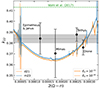 |
Fig. 1. Frequency variation in the Saturnian k2 Love number from astrometric data. Black points are the measurements that allow for different k2 values at each tidal forcing frequency, while the horizontal gray bar is the measurement found assuming a constant value of k2. The orange and blue lines are the dynamical tidal response for two different Saturn models, with thick and thin lines corresponding to higher and lower viscosities, respectively. The dashed green line shows the hydrostatic k22 = 0.4130 computed by Wahl et al. (2017). |
For the tidal driving, we approximated satellite tidal potentials as point-mass potentials expanded in spherical harmonics up to degree ℓ = 12 and computed k22 Love numbers as the real part of the ratio given in Eq. (5) (for ℓ = m = 2). Including multiple harmonic degrees in the expansion of the tidal potential leads to some ambiguity in the definition of a response function defined for oblate bodies since one spherical harmonic of the tidal potential can drive another in the response (Dewberry & Lai 2022), but this effect is minimal for sectoral (ℓ = m) harmonics.
Figure 1 compares the predicted k22 values to our measurements. Both models are compatible with the measured values within their uncertainties. The models predict a parabolic dependence of k22 on the tidal forcing frequency, with a minimum value near the forcing frequency of Mimas. This arises due to the Coriolis force on the tidal bulge, which is dominated by Saturn’s fundamental modes (see Dewberry et al. 2021; Idini & Stevenson 2021). This dynamical tidal effect is necessary to explain Juno measurements of Jupiter’s tidal bulge raised by Io (Lin 2023; Dewberry 2023; Dhouib et al. 2024) and should be present inside Saturn as well. Unfortunately, the substantial uncertainties of the measurements do not allow us to clearly detect this dynamical tidal effect. However, we note that the measured k22 is inconsistent with the value predicted by Wahl et al. (2017), who neglected dynamical tidal effects (i.e. they predicted the value of k22 at a tidal forcing frequency of zero). Similar to measurements for Jupiter, dynamical tidal effects likely explain the lower-than-expected value of k22 compared to predictions at a zero tidal forcing frequency.
In addition to the parabolic trend in k22, the models also predict sharp, localized variations in this trend at certain tidal frequencies. They correspond to resonances with gravito-inertial modes of the planet, which enhance the tidal response and alter the value of k22 near the mode frequencies. These resonant frequencies are sensitive to the planetary model (in particular the stable stratification and rotation profiles), so a detection of resonant variations in k22 would provide strong constraints on the internal structure of Saturn. For instance, both models in Fig. 1 predict a sharp variation in k22 near the frequency of Tethys, which could account for its higher k22 value compared to the other moons if it is in a resonance lock with one of Saturn’s gravito-inertial modes. The measurements are not yet precise enough to robustly detect these resonant effects, but measuring them in the future is an exciting prospect for constraining Saturn’s internal structure and understanding whether resonance locking is occurring (Luan et al. 2018). Characterizing not just the real but also the imaginary parts of tidal Love numbers computed for realistic Saturn interior models would also help answer this question. Such a characterization introduces complications (Pontin et al. 2024) that are beyond the scope of this Letter, however, and we defer it to future investigations.
4. Conclusion
Using astrometric measurements of Saturn’s moons, we were able to quantify Saturn’s k2 Love number at four different tidal frequencies. The measurement was facilitated by co-orbital moons, whose orbits are perturbed by the tidal bulge raised by the co-orbiting companion. Our Love number measurements are compatible with a constant value, within the error bars of the observations. They are also consistent with predictions from numerical models of the tidal response of Saturn, including contributions from fundamental modes, gravito-inertial modes, and inertial waves. Slightly more accurate future measurements will allow for the detection of dynamical tidal effects, including the possibility of resonantly excited gravito-inertial modes, which would allow us to place strong constraints on the internal structure of Saturn.
Acknowledgments
J.W. Dewberry is supported by the Natural Sciences and Engineering Research Council of Canada (NSERC), [funding reference # CITA 490888-16]. Q. Zhang was supported by the National Natural Science Foundation of China (No. 12373073, No. U2031104).
References
- Acton, C. H. 1996, Planet. Space Sci., 44, 65 [Google Scholar]
- Cooper, N. J., Murray, C. D., Lainey, V., et al. 2014, A&A, 572, A43 [NASA ADS] [CrossRef] [EDP Sciences] [Google Scholar]
- Cooper, N. J., Lainey, V., Meunier, L. E., et al. 2018, A&A, 610, A2 [NASA ADS] [CrossRef] [EDP Sciences] [Google Scholar]
- Dewberry, J. W. 2023, MNRAS, 521, 5991 [NASA ADS] [CrossRef] [Google Scholar]
- Dewberry, J. W., & Lai, D. 2022, ApJ, 925, 124 [NASA ADS] [CrossRef] [Google Scholar]
- Dewberry, J. W., Mankovich, C. R., Fuller, J., Lai, D., & Xu, W. 2021, Planet. Sci. J., 2, 198 [NASA ADS] [CrossRef] [Google Scholar]
- Dhouib, H., Baruteau, C., Mathis, S., et al. 2024, A&A, 682, A85 [NASA ADS] [CrossRef] [EDP Sciences] [Google Scholar]
- French, R. G., McGhee-French, C. A., Lonergan, K., et al. 2017, Icarus, 290, 14 [Google Scholar]
- Idini, B., & Stevenson, D. J. 2021, Planet. Sci. J., 2, 69 [NASA ADS] [CrossRef] [Google Scholar]
- Iess, L., Militzer, B., Kaspi, Y., et al. 2019, Science, 364, aat2965 [Google Scholar]
- Lainey, V. 2016, Celest. Mech. Dyn. Astron., 126, 145 [NASA ADS] [CrossRef] [Google Scholar]
- Lainey, V., Dehant, V., & Pätzold, M. 2007, A&A, 465, 1075 [NASA ADS] [CrossRef] [EDP Sciences] [Google Scholar]
- Lainey, V., Karatekin, Ö., Desmars, J., et al. 2012, ApJ, 752, 14 [Google Scholar]
- Lainey, V., Jacobson, R. A., Tajeddine, R., et al. 2017, Icarus, 281, 286 [Google Scholar]
- Lainey, V., Noyelles, B., Cooper, N., et al. 2019, Icarus, 326, 48 [Google Scholar]
- Lainey, V., Casajus, L. G., Fuller, J., et al. 2020, Nat. Astron., 4, 1053 [Google Scholar]
- Lainey, V., Rambaux, N., Cooper, N., Dahoumane, R., & Zhang, Q. 2023, A&A, 670, L25 [NASA ADS] [CrossRef] [EDP Sciences] [Google Scholar]
- Lainey, V., Rambaux, N., Tobie, G., et al. 2024, Nature, 626, 280 [NASA ADS] [CrossRef] [Google Scholar]
- Lin, Y. 2023, A&A, 671, A37 [NASA ADS] [CrossRef] [EDP Sciences] [Google Scholar]
- Luan, J., Fuller, J., & Quataert, E. 2018, MNRAS, 473, 5002 [Google Scholar]
- Mankovich, C. R., Dewberry, J. W., & Fuller, J. 2023, Planet. Sci. J., 4, 59 [NASA ADS] [CrossRef] [Google Scholar]
- Miguel, Y., Guillot, T., & Fayon, L. 2016, A&A, 596, A114 [NASA ADS] [CrossRef] [EDP Sciences] [Google Scholar]
- Militzer, B., & Hubbard, W. B. 2013, ApJ, 774, 148 [NASA ADS] [CrossRef] [Google Scholar]
- Nettelmann, N., Movshovitz, N., Ni, D., et al. 2021, Planet. Sci. J., 2, 241 [NASA ADS] [CrossRef] [Google Scholar]
- Newhall, X. X., Standish, E. M., & Williams, J. G. 1983, A&A, 125, 150 [NASA ADS] [Google Scholar]
- Pontin, C. M., Barker, A. J., & Hollerbach, R. 2024, ApJ, 960, 32 [NASA ADS] [CrossRef] [Google Scholar]
- Porco, C. C., West, R. A., Squyres, S., et al. 2004, Space Sci. Rev., 115, 363 [NASA ADS] [CrossRef] [Google Scholar]
- Tajeddine, R., Cooper, N. J., Lainey, V., Charnoz, S., & Murray, C. D. 2013, A&A, 551, A129 [NASA ADS] [CrossRef] [EDP Sciences] [Google Scholar]
- Tajeddine, R., Lainey, V., Cooper, N. J., & Murray, C. D. 2015, A&A, 575, A73 [NASA ADS] [CrossRef] [EDP Sciences] [Google Scholar]
- Thompson, S. L. 1990, ANEOS–Analytic Equations of State for Shock Physics Codes, Sandia Natl. Lab. Doc. SAND89-2951, http://prod.sandia.gov/techlib/access-control.cgi/1989/892951.pdf [Google Scholar]
- Wahl, S. M., Hubbard, W. B., & Militzer, B. 2017, Icarus, 282, 183 [NASA ADS] [CrossRef] [Google Scholar]
- Zhang, Q. F., Zhou, X. M., Tan, Y., et al. 2021, MNRAS, 505, 5253 [NASA ADS] [CrossRef] [Google Scholar]
All Tables
Mean (ν) and standard deviation (σ) of the sample and line residuals (in pixels) for each satellite (Cassini-ISS data).
Mean (ν) and standard deviation (σ) of the sample and line residuals (in pixels) for each satellite (Cassini-ISS data).
All Figures
|
Fig. 1. Frequency variation in the Saturnian k2 Love number from astrometric data. Black points are the measurements that allow for different k2 values at each tidal forcing frequency, while the horizontal gray bar is the measurement found assuming a constant value of k2. The orange and blue lines are the dynamical tidal response for two different Saturn models, with thick and thin lines corresponding to higher and lower viscosities, respectively. The dashed green line shows the hydrostatic k22 = 0.4130 computed by Wahl et al. (2017). |
| In the text | |
Current usage metrics show cumulative count of Article Views (full-text article views including HTML views, PDF and ePub downloads, according to the available data) and Abstracts Views on Vision4Press platform.
Data correspond to usage on the plateform after 2015. The current usage metrics is available 48-96 hours after online publication and is updated daily on week days.
Initial download of the metrics may take a while.