| Issue |
A&A
Volume 670, February 2023
|
|
|---|---|---|
| Article Number | L25 | |
| Number of page(s) | 6 | |
| Section | Letters to the Editor | |
| DOI | https://doi.org/10.1051/0004-6361/202244757 | |
| Published online | 24 February 2023 | |
Letter to the Editor
Characterising the interior of five inner Saturnian moons using Cassini ISS data⋆
1
IMCCE, Observatoire de Paris, PSL Research University, CNRS, Sorbonne Université, Univ. Lille, Paris, France
e-mail: This email address is being protected from spambots. You need JavaScript enabled to view it.
2
Department of Physics & Astronomy, Queen Mary University of London, Mile End Rd, London E1 4NS, UK
3
Department of Computer Science, Jinan University, Guangzhou 510632, PR China
Received:
17
August
2022
Accepted:
5
January
2023
Abstract
Context. The Cassini-Huygens space mission provided a huge amount of data for the Saturnian system. While the mission ended in September 2017, there is still much information to be retrieved from the data.
Aims. Here, from their orbital motion, we infer the interior of the five inner Saturnian moons, Atlas, Prometheus, Pandora, Janus, and Epimetheus. Our results benefit from a recent study of the shape of these moons, which provides a much better estimation of their 3D shape and volume.
Methods. Using Cassini Imaging Science Subsystem (ISS) astrometric data, we again reduced the Cassini ISS images with an improved shape modelling. We then integrated the orbital motion of the inner Saturnian moons and solved for a large set of physical parameters for this system, including the masses and physical libration amplitudes of the moons.
Results. We obtain a density value (in g cm−3 with a 1σ error bar based on the digital terrain models and spherical harmonics available today) of 0.3935 ± 0.0033, 0.4873 ± 0.0026, 0.5045 ± 0.0017, 0.6233 ± 0.0015, and 0.6413 ± 0.0002 for Atlas, Prometheus, Pandora, Epimetheus, and Janus, respectively. We were able to determine the physical libration amplitudes of Prometheus, Pandora, Epimetheus, and Janus to be 0.98 ± 0.08, −5.2 ± 0.7, −6.0 ± 0.6, and −0.39 ± 0.16 (degrees and 1σ error bar), respectively. Our solutions for Epimetheus and Janus are in full agreement with a former estimation performed directly from the measurement of the rotation of these two moons.
Conclusions. We confirm the large porosity of these five moons and their increase in density as a function of their size. Our estimations of the physical librations of Prometheus, Pandora, Janus, and Epimetheus are consistent with a homogeneous interior, but for Pandora a heterogeneous interior is also plausible.
Key words: astrometry / planets and satellites: interiors
Our new astrometric data sets are only available at the CDS via anonymous ftp to cdsarc.cds.unistra.fr (130.79.128.5) or via https://cdsarc.cds.unistra.fr/viz-bin/cat/J/A+A/670/L25
© The Authors 2023
 Open Access article, published by EDP Sciences, under the terms of the Creative Commons Attribution License (https://creativecommons.org/licenses/by/4.0), which permits unrestricted use, distribution, and reproduction in any medium, provided the original work is properly cited.
This article is published in open access under the Subscribe to Open model. This email address is being protected from spambots. You need JavaScript enabled to view it. to support open access publication.
1. Introduction
The five inner moons of Saturn were likely formed at the Saturnian Roche limit, close to the current outer edge of the A ring (Charnoz et al. 2010) by a gradual accretion process, which may explain their low densities (Thomas et al. 2013). Assessing potential heterogeneity inside these objects could be very informative, and would help us to characterise the relative velocity of potential collisions during their formation process, or orbital evolution history, as they progress further away from Saturn as a result of their dynamical interaction with the rings.
Lainey et al. (2019) tried to estimate the amplitudes of the physical librations of Prometheus, Pandora, Epimetheus, and Janus using Cassini Imaging Science Subsystem (ISS) astrometric data. While these authors were able to constrain the amplitudes, they could not determine them precisely because of large error bars, with the exception of Pandora. To solve this issue, Lainey et al. (2019) suggested that a significant improvement may be expected by reducing the data again using a more accurate shape modelling than ellipsoids during the astrometric reduction process of ISS data. Recently, Rambaux et al. (2022) analysed the shape of the small moons of Saturn, and provided a description of their shapes using spherical harmonics, which is a convenient form for considering a more complex shape than the ellipsoid.
Here, we first reprocess the ISS data using 3D shape models from Rambaux et al. (2022). In addition, we use the modified moment algorithm (Zhang et al. 2021) to measure the astrometric positions of moons whose apparent diameter is too small for shape modelling. We then give the results of a similar analysis to that performed by Lainey et al. (2019), but this time using the updated astrometric data. Last but not least, thanks to Rambaux et al. (2022) we have a much more precise estimation of the shape of the inner Saturnian moons, which we used to determine their respective volume and uncertainty. This allowed us to obtain a level of precision in the density of these moons that has never previously been achieved.
2. Astrometric observations
We implemented the 3D shape modelling from Rambaux et al. (2022) in the Caviar software package (Cooper et al. 2018). Following Lainey et al. (2019), the data set was split into different subsets depending on the technique used for the determination of the centre of figure of the moons in the images. When the apparent diameter of the moon was above typically 3–4 pixels, we were able to provide a position of the centre of figure of the satellite using the limb-fitting method and complex shape modelling (see Fig. 1). In total, we were able to recompute 2635 astrometric positions with the updated limb-fitting method. For Prometheus, Pandora, Epimetheus, and Janus, images taken from relatively large distances were not used. Indeed, a first analysis showed that they did not provide any useful signal on the dynamics of these moons, taking into account the great accuracy of limb-fitted data. On the other hand, Atlas is smaller and only one-third of the astrometric images could be reduced using the limb-fitting technique. Hence, we tried reprocessing all other Atlas images using the modified moment algorithm (Zhang et al. 2021), which is an improvement to the usual Gaussian fit for photocentre determination. In total, we were able to properly reduce about 333 images with this technique, resulting in only a slight improvement to the astrometric residuals. While Zhang et al. (2021) observed a large improvement in Anthe’s astrometric residuals, it seems that the larger apparent size of Atlas (typically a few pixels) makes a difference. In particular, the phase correction applied in Caviar assumed a perfectly spherical shape, which is generally far from the case with these small moons. This rough approximation is most likely to be the dominating source of error in our photocentre determinations.
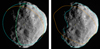 |
Fig. 1. Comparison between two methods to fit the centre of figure using Janus observation N1627319153_1 (resolution 0.6 km per pixel). On the left, we show the method used by Cooper et al. (2018). On the right, we show the new method relying on a complex 3D shape modelling. The vertical size of Janus on the image is about 325 pixels. The orange curve represents the equator of the moon. The cyan curve is the computed shape to be fitted to the image contour. |
3. Orbital fit
We carried out orbital dynamical modelling and fitting to the observations in a similar way to Lainey et al. (2019), with the additional improvement of including the Cassini Grand Finale estimate of the gravity field of Saturn (Iess et al. 2019). The gravity harmonics were still solved for, but were constrained to remain in agreement with the solution of Iess et al. (2019), within their given uncertainty. For convenience, we review our method and the relevant equations below, and refer the reader to Lainey et al. (2019) for further details.
3.1. Dynamical modelling
Using the NOE gravitational N-body code (Lainey et al. 2007, 2009; Lainey 2008), we fitted the full equations of motion (see Eq. (1)) to the astrometric observations described above, solving for the initial positions, velocities, and physical librations of Prometheus, Pandora, Janus, and Epimetheus, in addition to various global parameters, such as the masses, Cnp and Snp gravity coefficients, and polar orientation.
Our model included (i) gravitational interactions up to degree 2 in the expansion of the gravitational potential of the satellites (Table 2 from Lainey et al. 2019) and degree 10 for Saturn (Iess et al. 2019; (ii) gravitational perturbations from Mimas, Enceladus, Tethys, Dione Rhea, Titan, Hyperion, and Iapetus based on ephemerides from Lainey et al. (2020; (iii) the solar perturbation (where the masses of the inner planets and the Moon were incorporated into the solar mass), and Jupiter based on the DE430 ephemeris; (iv) the precession of Saturn; (v) tidal effects based on the Love number k2, neglecting dissipation; and (vi) relativistic corrections.
Following Lainey et al. (2007), the equation of motion for a satellite Pi may be expressed as
 (1)
(1)
where ri and rj are the position vectors of the satellite Pi and a perturbing body Pj (another satellite, the Sun, or Jupiter) with mass mj, respectively, subscript 0 denotes Saturn,  is the gravity field of body Pl at the position of body Pk (including planetary oblateness), GR are corrections due to general relativity (Newhall et al. 1983),
  is the force on Pl from the tides it raises on its primary body, and
  is the effect of tides raised by one moon on Saturn acting on another moon. In the absence of tidal dissipation, the latter two forces are given by Lainey et al. (2007, 2017):
 (2)
(2)
![Mathematical equation: $$ \begin{aligned}&\boldsymbol{F}^T_{ij} =\frac{3k_2Gm_jm_iR^5}{2r^5_i r^5_j}\left[-\frac{5(\boldsymbol{r}_i\cdot \boldsymbol{r}_j)^2\boldsymbol{r}_i}{r^2_i}+r^2_j\boldsymbol{r}_i+2(\boldsymbol{r}_i\cdot \boldsymbol{r}_j)\boldsymbol{r}_j\right]. \end{aligned} $$](/articles/aa/full_html/2023/02/aa44757-22/aa44757-22-eq6.gif) (3)
(3)
The physical libration of the moon Pi arises implicitly in the expression of  and
and  in Eq. (1). For more details, the reader may refer to Lainey et al. (2019), Eqs. (22) and (23).
The fitting process involved solving the variational equations for an unspecified parameter cl of the model to be fitted (e.g., r(t0),dr/dt(t0),Q…); see Lainey et al. (2012) for more details:
![Mathematical equation: $$ \begin{aligned} \frac{\partial }{\partial c_l}\left(\frac{\mathrm{d}^2\boldsymbol{r}_i}{\mathrm{d}t^2}\right)=\frac{1}{m_i}\left[\sum _j\left(\frac{\partial \boldsymbol{F}_i}{\partial \boldsymbol{r}_j}\frac{\partial \boldsymbol{r}_j}{\partial c_l}+\frac{\partial \boldsymbol{F}_i}{\partial \dot{\boldsymbol{r}}_j}\frac{\partial \dot{\boldsymbol{r}}_j}{\partial c_l} \right)+\frac{\partial \boldsymbol{F}_i}{\partial c_l}\right]. \end{aligned} $$](/articles/aa/full_html/2023/02/aa44757-22/aa44757-22-eq9.gif) (4)
(4)
In the above expression, Fi is the right-hand side of Eq. (1) multiplied by mi. The partial derivatives of the solutions with respect to initial positions and velocities of the satellites and dynamical parameters were then computed by the simultaneous numerical solution of Eqs. (1) and (4), in a Saturn-centred frame with inertial axes based on the Earth mean equator of J2000.
To test the reliability of our fit, we considered additional perturbations (see Tables 1 and 2). Among other effects, we considered the influence of Mimas’s extended gravity field, the Saturnian nutations from the SAT427 SPICE kernel (Acton 1996), the Saturnian polar orientation determined by French et al. (2017), the use of the SAT427 ephemerides for the main moons, and the influence of higher-order gravity parameters for the inner moons under the homogeneity assumption.
Estimation of Gm (km3 s−2) for the moons.
Estimation of physical libration amplitudes (in degrees).
In summary, all our simulations involved solving simultaneously for the initial state vectors and masses of the moons, the masses and gravity field of Saturn, including zonal harmonics up to order 10, the orientation and precession of Saturn, and the physical librations for Prometheus, Panodra, Janus, and Epimetheus. No constraints were introduced in the fitting, except for Saturn’s gravity field at the value estimated by Iess et al. (2019) assuming their published 1σ uncertainty.
3.2. Weighting the data
Each observed astrometric data value has an inherent uncertainty in pixel units originating from the centre-of-figure determination. The Caviar software makes an estimate of this uncertainty, but this estimate does not take into account the uncertainty in the camera pointing direction, and more importantly, the real meaning of the Caviar uncertainty as a standard deviation (i.e., 1σ) is unclear. As a consequence, we instead followed the method used by Lainey et al. (2019) to estimate a 1σ uncertainty for each data point as accurately as possible. In particular, we rescaled the Caviar uncertainties using a scalar chosen to distribute about 66% of astrometric residuals to within a 1σ level for each satellite and coordinate value.
An additional issue to be taken into account was the redundancy of information coming from some ISS observation sequences: often data points existed within a relatively small time interval of each other (in this case, less than 30 min). This presented a particular problem in the data-weighting step, where biases could be introduced. Following Lainey et al. (2019), in order to mitigate this, the data were de-weighted by a factor  with N being the number of observations in the series.
ISS data were finally weighted using the root mean square (rms) of the astrometric residuals, coming from a first estimate of the positions of the moons based on our model, as an a priori constraint when fitting the data.
4. Volume uncertainties
Here, we present our approach to deriving the volume uncertainties. The spherical harmonics (SH) decomposition presented by Rambaux et al. (2022) is based on the digital terrain models (DTMs) built by Thomas & Helfenstein (2020). These DTMs are proposed as tesselated plate models with a spatial distribution of 2° ×2°. Rambaux et al. (2022) provided a detailed discussion of the limitations and the uncertainties on the shape based on the DTM. Notably, these authors constructed confidence limits on the shape models using limb measurements of these satellites. These were used by Rambaux et al. (2022) to deduce the maximum relevant degree for the decomposition and establish a robust uncertainty on the second-degree coefficients, which was the focus of this latter study. Here, in the present study, to estimate the confidence limit on the volume, we use a Monte Carlo propagation (500 iterations) where the uncertainty on each spherical harmonic coefficient is obtained by scaling its formal uncertainty as a function of the uncertainty of the second-degree coefficient A20. The uncertainties on the volumes are of the order of 50 km3 for Atlas and 1000–2000 km3 for the other bodies. Our final volume and uncertainty estimate for each moon are given in Table 1.
5. Results
Table A.1 provides the post-fit astrometric residuals for the five moons. In comparison with Lainey et al. (2019), the residuals are clearly better for Epimetheus and Janus, which is to be expected as these moons are the largest of those studied in this work. As a consequence, they should be the most affected by the ellipsoidal shape errors. As an example, Fig. A.1 shows the comparison between the Janus astrometric residuals from Lainey et al. (2019) and those of the present work.
Table 1 provides the Gm estimations of the five inner Saturnian moons studied in this work. The error bars are given at the 1σ level. To test the reliability of our solution, we performed many tests using different modelling conditions. These included the influence of the extended gravity field of Mimas; Saturn’s nutations; forcing the orientation of Saturn’s pole from the French et al. (2017) solution; using older Cassini orbit determinations; using different ephemerides for the main moons (and their respective masses); and introducing higher-order gravity fields for the inner moons. One clearly sees from Table 1 that these different simulations are in full agreement within the error bars. The global Gm solution given in Table 1 is the 1σ envelope of former solutions given in the table.
Table 1 also provides an estimate of the densities computed by combining the masses obtained by the astrometric data with the volume deduced from the surface decomposed in spherical harmonics. The computation of the volume uncertainties is described in Sect. 4. The Table 1 shows good agreement with the determination of Thomas & Helfenstein (2020) and density uncertainties are of the same order of magnitude. In Fig. 2, we show the improvement in densities between Lainey et al. (2019) and the present work. To make a fair comparison, we multiplied our error bars in Fig. 2 by a factor of 3 (three sigmas), because Lainey et al. (2019) gave very conservative uncertainties. We clearly see that the densities increase with object size, as expected from the effect of gravity-driven self-compaction.
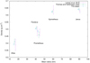 |
Fig. 2. Density variation of the inner Saturnian moons as a function of size. |
Table 2 provides our estimation of the physical librations of Prometheus, Pandora, Epimetheus, and Janus. Here again, the error bars are at the 1σ level, and our chosen solution is the envelope of all 1σ former solutions. The amplitudes of Epimetheus and Pandora are large, about 5 deg, while Prometheus presents a librational amplitude of 1 deg, and Janus 0.4 deg. The sign, or equivalently the libration phase, is positive for Prometheus and negative for the other satellites. The sign values depend on the values of the proper frequency with respect to the mean motion (e.g., Tiscareno et al. 2009; Rambaux et al. 2022). In addition, our solution for Janus and Epimetheus is in full agreement with the one obtained after directly measuring the rotation of these moons (Tiscareno et al. 2009). Moreover, they both stand well within 1σ of the homogeneous solution estimated by Rambaux et al. (2022). Our solution for Prometheus intersects with the homogeneous case at the 1.2σ level, which is reasonable and is consistent with the estimation from Thomas et al. (2018). On the other hand, the amplitude of libration for Pandora’s solution is well outside of the error bar given in Rambaux et al. (2022) or the value estimated in Thomas et al. (2018). Despite this large discrepancy, it is not possible to conclusively demonstrate the presence of heterogeneity in Pandora as discussed below.
6. Discussion
Rambaux et al. (2022) computed the libration amplitude of Saturn’s inner satellites taking into account the uncertainty on their shapes. Using a Monte Carlo approach, these authors calculated the Stokes coefficients C20 and C22, followed by the physical libration. The solutions reported in Rambaux et al. (2022) correspond to the 0.33 quantile around the median value. Figure A.2 shows the histogram of solutions for Pandora assuming a homogeneous interior. This histogram is strongly asymmetric and some solutions can even reach the large value of −7 deg, which is beyond the observed value. This behaviour is due to the strong non-linearity between the Stokes coefficients (calculated from the shape) and the amplitude of the libration when the physical libration is close to a resonance. This resonance is between the proper frequency and the mean motion. Now the solution for Pandora is high on the vertical asymptotic branch as shown in Fig. 9 of Rambaux et al. (2022). In addition, because of this proximity of resonance, very few heterogeneities are needed for the libration amplitude to increase rapidly (in absolute value) and reach the observed value. Thus, even if Pandora certainly shows a signature of heterogeneity, it is not possible to rule out the homogeneous solution, and a better precision in the shape would be necessary to clearly distinguish between these two possibilities.
7. Conclusion
We provide the most precise estimation of the densities of Atlas, Prometheus, Pandora, Epimetheus, and Janus obtained so far, confirming their very high porosity and the dependency of this quantity on the sizes of the moons. Moreover, we succeeded in inferring the amplitudes of the physical librations of the four largest inner moons. Our solutions are consistent with homogeneous interiors, although Pandora might present heterogeneity.
Acknowledgments
Q. Zhang was supported by the Joint Research Fund in Astronomy (grant no. U2031104) under cooperative agreement between the National Natural Science Foundation of China and Chinese Academy of Sciences.
References
- Acton, C. H. 1996, Planet Space Sci., 44, 65 [NASA ADS] [CrossRef] [Google Scholar]
- Charnoz, S., Salmon, J., & Crida, A. 2010, Nature, 465, 752 [NASA ADS] [CrossRef] [Google Scholar]
- Cooper, N. J., Lainey, V., Meunier, L. E., et al. 2018, A&A, 610, A2 [NASA ADS] [CrossRef] [EDP Sciences] [Google Scholar]
- French, R. G., McGhee-French, C. A., Lonergan, K., et al. 2017, Icarus, 290, 14 [Google Scholar]
- Iess, L., Militzer, B., Kaspi, Y., et al. 2019, Science, 364, aat2965 [Google Scholar]
- Lainey, V. 2008, Planet. Space Sci., 56, 1766 [NASA ADS] [CrossRef] [Google Scholar]
- Lainey, V., Dehant, V., & Pätzold, M. 2007, A&A, 465, 1075 [NASA ADS] [CrossRef] [EDP Sciences] [Google Scholar]
- Lainey, V., Arlot, J.-E., Karatekin, Ö., & van Hoolst, T. 2009, Nature, 459, 957 [Google Scholar]
- Lainey, V., Karatekin, Ö., Desmars, J., et al. 2012, ApJ, 752, 14 [Google Scholar]
- Lainey, V., Jacobson, R. A., Tajeddine, R., et al. 2017, Icarus, 281, 286 [Google Scholar]
- Lainey, V., Noyelles, B., Cooper, N., et al. 2019, Icarus, 326, 48 [Google Scholar]
- Lainey, V., Casajus, L. G., Fuller, J., et al. 2020, Nat. Astron., 4, 1053 [Google Scholar]
- Newhall, X. X., Standish, E. M., & Williams, J. G. 1983, A&A, 125, 150 [NASA ADS] [Google Scholar]
- Rambaux, N., Lainey, V., Cooper, N., Auzemery, L., & Zhang, Q. F. 2022, A&A, 667, A78 [NASA ADS] [CrossRef] [EDP Sciences] [Google Scholar]
- Thomas, P., & Helfenstein, P. 2020, Icarus, 344, 113355 [NASA ADS] [CrossRef] [Google Scholar]
- Thomas, P. C., Burns, J. A., Hedman, M., et al. 2013, Icarus, 226, 999 [NASA ADS] [CrossRef] [Google Scholar]
- Thomas, P. C., Tiscareno, M. S., & Helfenstein, P. 2018, in Enceladus and the Icy Moons of Saturn, eds. P. M. Schenk, R. N. Clark, C. J. A. Howett, A. J. Verbiscer, & J. H. Waite, 387 [Google Scholar]
- Tiscareno, M. S., Thomas, P. C., & Burns, J. A. 2009, Icarus, 204, 254 [NASA ADS] [CrossRef] [Google Scholar]
- Zhang, Q. F., Zhou, X. M., Tan, Y., et al. 2021, MNRAS, 505, 5253 [NASA ADS] [CrossRef] [Google Scholar]
Appendix A: Additional material
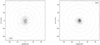 |
Fig. A.1. Astrometric residuals after a fit between the model and the ISS observations for Janus in sample and line coordinates rescaled in km. On the left are the residuals from Lainey et al. (2019). On the right are the residuals using reprocessed data. |
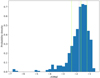 |
Fig. A.2. Histogram of the physical libration for Pandora. The mean value is the vertical grey line, the median value is the green line, and the 0.33 quantile range is represented by the green dotted lines. |
Mean (ν) and standard deviation (σ) on sample and line residuals from the calculated body centre in pixels for each satellite (Cassini-ISS data). N is the number of observations by satellite considered and for each coordinate. Observations with residuals higher than 2.5 pixels were discarded. NAC stands for the Narrow Angle Camera of the Cassini Imaging Science Subsystem.
All Tables
Mean (ν) and standard deviation (σ) on sample and line residuals from the calculated body centre in pixels for each satellite (Cassini-ISS data). N is the number of observations by satellite considered and for each coordinate. Observations with residuals higher than 2.5 pixels were discarded. NAC stands for the Narrow Angle Camera of the Cassini Imaging Science Subsystem.
All Figures
|
Fig. 1. Comparison between two methods to fit the centre of figure using Janus observation N1627319153_1 (resolution 0.6 km per pixel). On the left, we show the method used by Cooper et al. (2018). On the right, we show the new method relying on a complex 3D shape modelling. The vertical size of Janus on the image is about 325 pixels. The orange curve represents the equator of the moon. The cyan curve is the computed shape to be fitted to the image contour. |
| In the text | |
|
Fig. 2. Density variation of the inner Saturnian moons as a function of size. |
| In the text | |
|
Fig. A.1. Astrometric residuals after a fit between the model and the ISS observations for Janus in sample and line coordinates rescaled in km. On the left are the residuals from Lainey et al. (2019). On the right are the residuals using reprocessed data. |
| In the text | |
|
Fig. A.2. Histogram of the physical libration for Pandora. The mean value is the vertical grey line, the median value is the green line, and the 0.33 quantile range is represented by the green dotted lines. |
| In the text | |
Current usage metrics show cumulative count of Article Views (full-text article views including HTML views, PDF and ePub downloads, according to the available data) and Abstracts Views on Vision4Press platform.
Data correspond to usage on the plateform after 2015. The current usage metrics is available 48-96 hours after online publication and is updated daily on week days.
Initial download of the metrics may take a while.