| Issue |
A&A
Volume 667, November 2022
|
|
|---|---|---|
| Article Number | A152 | |
| Number of page(s) | 19 | |
| Section | Extragalactic astronomy | |
| DOI | https://doi.org/10.1051/0004-6361/202142779 | |
| Published online | 21 November 2022 | |
Reconstructing AGN X-ray spectral parameter distributions with Bayesian methods
I. Spectral analysis
Department of Astronomy, University of Geneva, ch. d’Écogia 16, 1290 Versoix, Switzerland
e-mail: This email address is being protected from spambots. You need JavaScript enabled to view it.
Received:
29
November
2021
Accepted:
10
May
2022
Abstract
X-ray spectra of active galactic nuclei (AGN) consist of several different emission and absorption components. To determine the spectral parameters, these components are often fitted manually with models chosen on a case-by-case basis. However, this approach has two problems. First, it becomes very hard for a survey with a large number of sources. Second, when the signal-to-noise ratio (S/N) is low, there is a tendency to adopt an overly simplistic model, biasing the parameters and making their uncertainties unrealistic. We developed a Bayesian method for automatically fitting AGN X-ray spectra obtained by XMM-Newton with a consistent and physically motivated model. Our model includes all spectral components, even when the data quality is low. We used a physical model for the X-ray background and an empirical model for the non-X-ray background. Noninformative priors were applied on the parameters of interest, the photon index (Γ) and the hydrogen column density (NH), while informative priors obtained from deep surveys were used to marginalize over the parameter space of the nuisance parameters. To improve speed, we developed a specific spectral extraction and fitting procedure. We tested this method using a realistic sample of 5000 spectra, which was simulated based on our source model, reproducing typical population properties. Spectral parameters were randomly drawn from the priors, taking the luminosity function into account. Well-constrained or meaningful posterior probability density distributions (PDFs) were obtained for the most relevant spectral parameters, for instance, NH, Γ, and LX, even at low S/N, but in this case, we were unable to constrain the parameters of secondary components such as the reflection and soft excess. As a comparison, a maximum-likelihood approach with model selection among six models of different complexities was also applied to this sample. We find clear failures in the measurement of Γ in most cases, and of NH when the source is unabsorbed (NH < 1022 cm−2). The results can hardly be used to reconstruct the parent distributions of the spectral parameters, while our Bayesian method provides meaningful multidimensional posteriors that will be used in a subsequent paper to infer the population.
Key words: galaxies: active / X-rays: galaxies / methods: data analysis / methods: statistical
© L. Ge et al. 2022
 Open Access article, published by EDP Sciences, under the terms of the Creative Commons Attribution License (https://creativecommons.org/licenses/by/4.0), which permits unrestricted use, distribution, and reproduction in any medium, provided the original work is properly cited.
This article is published in open access under the Subscribe-to-Open model. This email address is being protected from spambots. You need JavaScript enabled to view it. to support open access publication.
1. Introduction
Active galactic nuclei (AGN) are thought to be powered by accretion of galactic matter onto supermassive black holes (SMBHs) in the centers of galaxies. Extremely strong radiation is produced from the accretion power, rivaling and sometimes outshining the collective emission of all the stars in their host galaxy. The tremendous amount of energy released by AGN may also influence their surroundings, namely the host galaxies or galaxy clusters (for a review, see Fabian 2012). The co-evolution of AGN and host galaxies was first discovered in the tight correlation between the SMBH masses and the properties of the host galaxy bulges, such as the luminosity (Magorrian et al. 1998) or velocity dispersion (Gebhardt et al. 2000; Ferrarese & Merritt 2000), and was then further detected in the similar histories of AGN accretion and star formation, which both peak at a redshift around 1–2 (Hopkins et al. 2006; Silverman et al. 2008; Aird et al. 2015). However, the details of the interplay between AGN and galaxies are still unclear (Kormendy & Ho 2013). Therefore, much effort has been devoted to studying the demographics of AGN properties, such as the luminosity, accretion rate, and black hole mass, which can be used to reconstruct the mass accretion history of SMBHs in the Universe.
A reliable measurement of the cosmological build-up of SMBHs requires a complete census of AGN activities. However, this is very difficult to conduct due to the multifaceted AGN radiation properties at all wavelengths, which result from the large number of physical processes that produce the different components of the total AGN emission, and from the presence of obscuring material in the vicinity of AGN that strongly affects the direct observations by absorbing and reprocessing the primary radiation. A large fraction of AGN (up to about 70%, depending on luminosity) is obscured by the intervening gas and dust (Burlon et al. 2011; Ueda et al. 2014; Aird et al. 2015; Buchner et al. 2015; Ricci et al. 2015; Ananna et al. 2019); it is therefore very important to characterize the full distribution of the absorbing column density and its dependence on redshift and AGN luminosity to uncover the complete AGN population.
Each method of AGN detection and selection has different biases (Hickox & Alexander 2018). Among them, X-ray surveys are particularly efficient for three main reasons: first, X-ray emission is ubiquitous in AGN (Avni & Tananbaum 1986; Brandt et al. 2000; Gibson et al. 2008); second, X-rays are able to penetrate a large amount of obscuring gas and dust along the line of sight because the photoelectric cross-section decreases with increasing photon energy (Wilms et al. 2000); and last, X-ray emission from the host galaxies is usually much weaker than that of the AGN, therefore X-rays are less diluted by stellar light than optical or IR surveys, for instance (Maccacaro et al. 1988).
X-ray spectra of AGN are intrinsically very complex, including the X-ray power-law continuum, which is predominately produced by the inverse Compton scattering of disk UV/optical photons in a hot corona very close to the SMBH (Blandford et al. 1990; Zdziarski et al. 1995, 1996; Krolik 1999), an excess of soft X-ray emission below 1–2 keV (Arnaud et al. 1985; Singh et al. 1985), the reflection of the primary X-ray power law by circumnuclear material (Pounds et al. 1990; Nandra & Pounds 1994), the scattering by warm fully ionized gas, located at a relatively large distance to the center of AGN (Bianchi et al. 2006; Guainazzi & Bianchi 2007), and thermal emission from diffuse plasma in the host galaxy (Iwasawa et al. 2011). Therefore, they may show different characteristics in different cases, such as strong reflection in absorbed spectra or obvious soft excess in unabsorbed ones.
However, these features are very often difficult to detect or constrain in a wide survey; in a typical survey, most sources have low signal-to-noise ratios (S/N), so that we are most likely to detect only the main components. To cope with this difficulty, the classical approach attempts to adapt the chosen spectral model to the quality of the spectra at hand. One starts with the simplest model, and then visually inspects the residuals to assess if more components are needed. For example, Ricci et al. (2017) used more than 20 models to fit a set of about 800 individual sources. However, this approach is hardly applicable to survey data including a large number sources. For instance, the XXL survey has about 22 000 X-ray point sources (Pierre et al. 2016), and the eROSITA all-sky survey (eRASS; Merloni et al. 2012) will produce a sample of about three million X-ray selected AGN (Kolodzig et al. 2013). Moreover, in the case of low S/N, even an overly simplistic model may achieve statistically satisfactory fits (Tozzi et al. 2006; Corral et al. 2011). Adopting an unrealistic model may introduce biases and provide unrealistic errors in recovering the main parameters, for example, hydrogen column density (NH), photon index (Γ), and X-ray luminosity (LX). An example to illustrate this point is shown in Sect. 2.4. Therefore, a consistent, physically motivated model and an automatic fitting procedure are required to fit AGN spectra that are extracted from large X-ray surveys.
In this paper we develop a new approach to analyzing the AGN X-ray spectral properties based on Bayesian inference, which allows us to properly propagate the uncertainties of components that are difficult to measure by marginalizing over them. The posteriors are computed with a nested-sampling algorithm to correctly deal with multimodal posteriors. Our goal is to devise a method that is capable of fitting the AGN X-ray spectra from about 0.5 to 12 keV automatically with a consistent, physically motivated model without the need of model comparison and selection. At the same time, the method must be able to determine the most relevant spectral parameters (NH, Γ, and LX) without strong bias even at low S/N. The final goal of our study is to reconstruct the parent distributions of the spectral parameters from their posteriors, which is addressed in Ge et al. (2022; hereafter Paper II). Throughout the paper, we consider the case of XMM-Newton (Jansen et al. 2001), but the principles can be adapted to any other X-ray instrument with adequate changes.
2. AGN X-ray spectral modeling
2.1. Components of X-ray emissions in AGN
At least five components contribute to the total X-ray spectra of AGN: the primary emission, soft excess, reflection, scattering in a warm plasma, and emission from thermal plasma in the galaxy. The primary emission is usually the dominant component, while the others are less luminous and more difficult to detect. In addition, the emitted spectrum is usually absorbed by gas and dust along the line of sight, both within the AGN and in our own galaxy. The detectability of the components depends strongly on the distribution of circumnuclear material in the AGN, which affects reflection and scattering.
2.1.1. Primary emission
The intrinsic X-ray emission from AGN is thought to be due to optical and UV photons from the accretion disk that are inverse-Compton scattered by high-energy electrons in a hot (kT ∼ 100 keV), optically thin (τ ∼ 0.5) corona (Blandford et al. 1990; Zdziarski et al. 1995, 1996; Krolik 1999) in the vicinity of the SMBH. Some recent works suggest that the corona can be optically thick, although this depends on the assumed geometry (Lanzuisi et al. 2019; Baloković et al. 2020). We fit this component using a redshifted power-law component with a high-energy cutoff with zcutoffpl (xspec model; Arnaud et al. 1996). Here the cutoff energy was fixed arbitrarily to 300 keV (Baloković et al. 2020), but because we only considered X-ray emission below ∼10 keV the chosen energy is irrelevant. The free parameters of this component are the photon index (Γ) and the normalization (F), which is defined as the intrinsic flux of the cutoff power law in the 2 to 10 keV band.
2.1.2. Soft excess
An excess of X-ray emission below 1–2 keV, called soft excess, is widely detected in AGN X-ray spectra (Piconcelli et al. 2005; Bianchi et al. 2009; Scott et al. 2012), although its origin remains debated. Possible explanations include blurred ionization reflection (Crummy et al. 2006; Fabian et al. 2009) or inverse Comptonization of disk photons in a warm, optically thick plasma (Mehdipour et al. 2011; Done et al. 2012; Boissay et al. 2014). Regardless of the origin of this component, we modeled it using a redshifted Bremsstrahlung (zbrem), which provides a simple phenomenological representation of its smooth spectral shape. In addition, the same shape has been used in Boissay et al. (2016), which provides us with a distribution of the soft-excess strength in nearby sources. The soft-excess strength is defined as the flux ratio of the Bremsstrahlung in the 0.5–2 keV band and the primary power law in the 2–10 keV band (Boissay et al. 2016). We parameterized the soft-excess strength with a multiplicative constant (q), which links the normalization of zbrem to the normalization parameter of zcutoffplF. Ricci et al. (2017) used another phenomenological model with a black body to model the soft-excess component, and obtained a good measurement of its temperature: 0.110 ± 0.003 keV. We therefore fixed the temperature in our zbrem model at 0.204 keV, which gives the best fit to a black body at 0.110 keV in the considered energy range. q is then the only free parameter of the soft excess.
2.1.3. Reflection
The primary X-ray emission from the inner region of the AGN can be reprocessed by reflection on circumnuclear material, including the disk, broad-line region, and torus (Pounds et al. 1990; Nandra & Pounds 1994). We used pexmon (Nandra et al. 2007) to model the reflection component, assuming a disk geometry and reflection with self-consistently generated fluorescence lines Fe Kα, Fe Kβ, and Ni Kα, as well as the Fe Kα Compton shoulder (Nandra et al. 2007). The true reflection spectrum depends on the precise shape and gas content of the reflector, but the expectation is that reflection will peak above 10 keV in all reasonable geometries and densities. Constraining the true shape of the reflection component would require deep hard X-ray observations, which cannot be done with XMM-Newton alone. Hence, pexmon was used as a model-independent description of the reflected component. The photon index, normalization, and cutoff energy were linked to those of the primary power law, and the inclination angle and the metallicity were fixed to 60° and 1, respectively. Therefore the only free parameter of the reflection is the reflection fraction (R) relative to an infinite disk.
2.1.4. Scattering
Primary power law and soft-excess emission escaping from the central engine can be scattered by fully ionized, optically thin gas relatively far away from the center of the AGN (Bianchi et al. 2006; Guainazzi & Bianchi 2007). The fully ionized plasma acts as a mirror, and the shape of the scattered component remains essentially unchanged. Its flux is typically a few percent (< 10%) of the incoming radiation, however, because the gas is optically thin and intercepts only a small fraction of the line of sights (Ueda et al. 2007). We added a multiplicative constant fscatter to the sum of the scattered zcutoffpl and zbrem without absorption from the torus to renormalize the flux. fscatter is the only free parameter of this component.
2.1.5. Absorption
Intrinsic absorption of the X-ray radiation is caused by two effects: the photoelectric absorption modeled with zphabs, and Compton scattering modeled with cabs. We linked the hydrogen column density NH of these two absorption models, which is the only free parameter. The absorption only affects emission from the inner region of the AGN, therefore it was applied on the primary power law and on the soft excess alone.
2.1.6. Thermal emission
Thermal emission coming from diffuse plasma in the host galaxy of the AGN (Iwasawa et al. 2011), originating, for example, from star-forming regions, is modeled with a collisionally ionized plasma (apec). The free parameters were the temperature of the plasma (kT) and its intrinsic luminosity lumin in the 2–10 keV band. The default normalization parameter was converted into luminosity using the convolution model clumin.
2.1.7. Full model
The total AGN emission was then further absorbed by the gas in our galaxy. We modeled this absorption using TBabs (Wilms et al. 2000). Compared to phabs, which contains only the gas component, TBabs also includes dust, so it is a better model for absorption in our own galaxy. For a real survey, Galactic NH is fixed for each source to the value at its sky coordinates, for instance, using the HI4PI Map (HI4PI Collaboration 2016). In the end, the full model, which has eight free parameters, is expressed (in xspec notation) as follows:
TBabs × (zphabs × cabs × (zcutoffpl + q × zbremss) + clumin × apec + pexmon
+ fscatter × (zcutoffpl + q × zbremss)).
2.2. Classic spectral modeling
The complexity of X-ray spectra of AGN, as demonstrated by the number of free parameters, requires high data quality to fully characterize all the components. However, wide surveys designed to observe a large number of AGN to study their population properties are dominated in number by faint sources with modest S/N. For instance, more than 90% of the sources in the XXL survey have an S/N lower than 3 (3XLSS catalogue; Chiappetti et al. 2018). Consequently, the full physical model is too complex for most of the spectra obtained in wide surveys.
A common practice in the study of AGN X-ray spectra is to optimize some statistics, for instance, χ2 or C-stat (Cash 1979), that is linked to the likelihood of a given parameter set. The best-fit parameters are then obtained using a maximum-likelihood (ML) optimization. However, when the number of free parameters is large compared to the S/N, the likelihood function is relatively flat over a large fraction of the parameter space, such that the position of the likelihood peak is sensitive to statistical fluctuations, making the ML optimization unstable.
To address the conflict between complexity of the model and low quality of the data, the model is usually simplified to include only the main components. Depending on the quality and characteristics of the spectrum, more complex models can be adopted. For example, we selected two sources from the 1000 brightest point source catalog of the XXL survey (Fotopoulou et al. 2016) and fit them using xspec. The first source (3XLSS J022915.6-044217) has a simple spectrum with a medium to high S/N of 4.8 and an exposure time of 5.4 ks. When we take the pn spectrum as an example, which has 122 spectral data counts and at least five counts per bin, it can be well fit using a simple power-law model with acceptable statistics (32.27 χ2 and 29.42 C-stat using 39 bins), as shown in Fig. 1. The data do not require more parameters, so that parameters such as Γ and NH are obtained from this simple fit. The second spectrum, from the Seyfert 2 galaxy NGC 788 (3XLSS J020106.4-064859, exposure time 10.0 ks), has a much higher S/N (41) and shows many more spectral features, for example, a highly absorbed primary power law and a strong reflection with an iron emission line, as shown in the bottom panel of Fig. 1. This object is the brightest point source in the XXL north field (Chiappetti et al. 2018), with a 2–10 keV flux of 1.4 × 10⁻¹² erg s−1 cm−2. For this source, it is necessary to apply the full model (Sect. 2.1.7), and each free parameter can be well fit, with the exception of the soft excess, which is completely absorbed1.
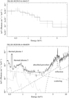 |
Fig. 1. Unfolded energy spectra (eufs) of two sources from the XXL-1000-AGN sample (Fotopoulou et al. 2016) that show very different spectral complexities. Top panel: 3XLSS J022915.6-044217. Bottom panel: 3XLSS J020106.4-064859 (NGC 788). The simple spectrum can be fit with a simple power-law model, while the complex spectrum requires the full model. In the bottom panel different components of the spectrum are shown by dashed lines. They are identified with text. |
Although it is able to describe the spectra of the sources of interest adequately, the model selection approach faces one important problem: a specific model for each source needs to be chosen. One can start with the simplest model and increase the model complexity depending on the improvement in the fit, as determined from an F-test, for instance, until the spectrum is well modeled. However, in a survey in which most sources have moderate fluxes, most sources are fitted with simple models (Tozzi et al. 2006; Corral et al. 2011). Consequently, the contributing but insignificant components are often ignored, resulting in a biased inference of the parameters (see an example in Sect. 2.4).
2.3. Bayesian approach
Instead of the classical approach described above, which requires model selection, a Bayesian X-ray spectral analysis approach can be adopted. The main differences with the ML approach are first, that each parameter is conditioned by prior knowledge, and second, that the result of the fitting process is a fully multivariate distribution, namely the posterior, and not just a best solution with errors.
A Bayesian model of the X-ray spectra consists of the determination of the posterior probability P(Θ|y), with Θ being the set of parameters and y the X-ray spectrum, using Bayes’ theorem,
 (1)
(1)
where P(Θ) is the prior probability of the set of parameters Θ, and P(y|Θ) is the likelihood of the observed data assuming the parameter set Θ. P(y) is the model evidence and can be ignored because all integrated probabilities give 1. We can then marginalize over the parameters of the less important components (i.e., sum the probabilities over all possible values of these parameters, e.g., all parameters except for Γ, NH , and F) to propagate the uncertainty on the exact spectral shape of the source to the posterior distributions of the parameters of interest, even if they have little effect on the likelihood,
 (2)
(2)
The Bayesian approach introduced here means that model selection is no longer required as long as meaningful priors are used, and we can apply a consistent model to all the spectra. This avoids the potential biases that may be introduced by an overly simplistic model (see Sect. 2.4 below).
2.4. Effect of the secondary components
To illustrate the effect of hidden parameters, we simulated a spectrum with XMM-Newton based on our full model (Sect. 2.1.7) using the xspec command fakeit. The input parameters were Γ = 2.1, F = 1.0 × 10⁻¹² ergs cm−2 s−1, NH = 1.0 × 1022 cm−2, q = 0.1, kT = 0.9 keV, lumin = 1039.5 erg s−1, R = 0.1, and fscatter = 0.08. We used the response and auxiliary files of a source in the XXL-1000-AGN sample (3XLSS J022915.6-044217; Fotopoulou et al. 2016) as a template, with 10 ks exposure time and 8.2 × 10⁻² ± 2.9 × 10⁻³ s−1 net count rate. The background was neglected in this case. The spectrum was fit with the full model and a simple model using xspec, as shown in the top two panels of Fig. 2. The simple model was a power law with photoelectric absorption (zphabs × zcutoffpl) and had only three free parameters: NH, Γ, and the normalization of the power law. The redshift was fixed to the chosen value (0.1) for both models. The minimum C-stat values of the two fits are close to one another. They are 138.7 for the full model and 152.0 for the simple one, using the same 148 data bins and hence 140 and 145 degrees of freedom (d.o.f), respectively.
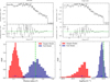 |
Fig. 2. Comparison between fits with models of different complexity. Top panels: best fit of a simulated spectrum using the full model (left) and the simple model (right). The residuals are plotted below. Bottom panels: posteriors of Γ (left) and NH (right) fitted with the full model (light purple) and the simple model (red). The dashed green lines show the input values. The blue points are medians of the posteriors with 68% credible intervals. |
We used the Bayesian information criterion (BIC; Schwarz 1978), as well as the Akaike information criterion (AIC; Akaike 1974), to compare these two models. The BIC values were calculated by  , where k is the number of free parameters, n is the number of data points, and
  is the maximum likelihood. As defined in Cash (1979),
  . We can find that the BIC of the full model is 178.7, while that of the simple model is 167.0, which means that the simple model is formally preferred. The AIC gives 154.7 and 158.0, respectively, as calculated by
  , which are not statistically different. We might conclude that fitting with the simple model is adequate based on these results.
However, in this case, but also in reality, we know that the real model does contain secondary components such as soft excess and reflection. The bottom panels of Fig. 2 show marginalized posteriors of Γ and NH obtained using MultiNest (see Sect. 3.4.2) with the two models. Noninformative priors were applied for the two main parameters, and the priors of other parameters for the full model are presented in Sect. 3.4.1. The simple model fails to recover the true parameters, fitting an absorbed soft spectrum with an unabsorbed hard solution. The full model, on the other hand, is able to retrieve the correct parameters. In the Bayesian framework, applying the simple model can be interpreted as applying the full model with very strong but incorrect priors that restrict secondary components to be zero. These strong assumptions bias the measurements and induce unrealistically small error bars on the parameters of interest. We conclude that it is necessary to analyze every AGN spectrum with the full model, even when the spectrum does not show clear evidence of the presence of additional components.
3. Spectral analysis
To be able to treat AGN spectra with their full complexity, we developed an alternative fitting approach based on Bayesian statistics. Because a Bayesian analysis can be very computationally expensive, we adapted the whole spectral analysis process, which we describe here in detail. In an analysis of real data, we assume that clean event lists are already available.
3.1. Spectral extraction
The standard way of extracting AGN X-ray spectra is to directly extract from the event files. Redistribution matrix file (RMF) and ancillary response file (ARF) are computed individually for each source to take the vignetting and detector nonuniformities into account. However, this approach leads to a very complex likelihood function because it requires the extraction and separate fitting of several spectra of the same source, which are taken in different exposures with different instruments on board XMM-Newton. For efficiency reasons, we simplified the process by stacking images of all the pointings for a given instrument to make mosaics in different energy bands, depending on the spectral resolution we want. The energy bands we used are listed in Table 1. They can be adjusted. We selected this binning because it is close to a uniform distribution in log-scale, except for two bins, which were intentionally set to 1.3–1.9 keV and 7.2–9.2 keV because of the Al K and Si K fluorescence emission lines at 1.5 and 1.7 keV for both pn and MOS, and those of Cu Kα, Ni Kα, and Zn Kα around 8 keV for pn (see the XMM-Newton User Handbook2).
Energy bands used for imaging and spectral extraction.
Spectral extraction was then performed directly on the mosaics by applying aperture photometry on the narrow-band images listed in Table 1. The MOS1 and MOS2 instruments are considered to be identical, which means that we worked with one pn mosaic and one MOS mosaic. The source spectra were extracted by counting the number of photons within a circular region around each source, and the background spectra were extracted from an annulus located outside of the source region. The neighboring catalog sources were masked to avoid contaminating the background region. The vignetting-corrected exposure maps were used to determine the local effective exposure time, which allowed us to use on-axis RMF and ARF files for all sources. The on-axis response files for pn and MOS were rebinned to match the energy band definition listed in Table 1 and then multiplied in each band by the local effective exposure time to take the dependence of the vignetting curve on energy into account. The C++ code implementing our spectral extraction technique is entitled xphot, and it is publicly distributed alongside this series of papers3.
The first advantage of this approach is that it is much more efficient to create only one consistent set of RMF and ARF than to create many local ones, especially when multiple pointings are combined. Second, it gives us a consistent energy binning for all the spectra, which, together with the constant RMF and ARF, enables us to perform the spectral fitting without xspec by constructing a single redistribution matrix. This accelerates the fitting process by a large factor. Details are presented in Sect. 3.4.2. The use of this technique comes at the price of losing some information because of the relatively coarse spectral binning. However, the loss of information is relevant only for the brightest sources because in faint sources, the uncertainties on the parameters become large and will hide any difference. Moreover, we show in Sect. 3.4.3 that the impact is minimum even for bright sources. In the typical situation of a survey, most sources have a relatively low S/N, such that the loss of information is negligible.
3.2. Background modeling
An important feature of X-ray spectra is that spectral bins typically contain a small number of counts and therefore follow Poisson statistics. To take the properties of the background into account in the fits, most previous works used background spectra obtained from source-free regions and subtracted the rescaled background spectra from the source spectra. However, the difference between two Poisson variables is no longer distributed like a Poisson variable, which can lead to severe biases. Instead of subtracting the background, we describe the background spectrum using a physically motivated model and fit the total spectra of the source and of the background simultaneously using both the source and background components in the former case and only the background components in the latter, preserving the Poisson statistics. We separately model the X-ray background (XB) and the non-X-ray background (NXB), and our background model is described in the following.
3.2.1. X-ray background
The XB was generated by photons from X-ray sources other than the source of interest. We modeled it with three components that represent the Local Bubble, the Galactic halo, and the cosmic X-ray background (CXB) as follows (in xspec notation):
constant × (apec + TBabs × (apec + constant × powerlaw)).
The first constant is a scaling factor that takes the different extraction areas for the source and background spectra into account. It was fixed for each source. The photoelectric absorption caused by our Galaxy was modeled using TBabs, as in the source model (see Sect. 2.1.7). The first apec model was the emission from the Local Bubble; its temperature was fixed to 0.11 keV (McCammon et al. 2002) and, being local, was unabsorbed. The other two components were absorbed by the same galactic NH column density as the source. The emission from the Galactic halo was taken into account by an absorbed apec with the temperature fixed to 0.22 keV (McCammon et al. 2002). The absorbed power law represents the cosmic X-ray background, which is thought to result from the unresolved AGN population (Moretti et al. 2003; Lehmer et al. 2012). The photon index of this power law was fixed to 1.46 following De Luca & Molendi (2004). While the shapes of these three components were fixed, their normalization parameters can be determined for each source using ROSAT data. We extracted the ROSAT spectrum in the survey field, using the HEASARC X-ray background tool4 (Sabol & Snowden 2019), and fit it with the model above. The normalization parameters of the Local Bubble and Galactic halo were then fixed to the best-fit values. The CXB can vary on small scales, however, so that its normalization (the second constant) remained free in subsequent fits to the source spectrum, but was constrained to be close to the best-fit value (see Sect. 3.4.1), which is the only free parameter of the XB model.
3.2.2. Non-X-ray background
The NXB consists primarily of secondary electrons caused by the interaction of charged high-energy particles with the spacecraft. Because the high-energy particles are going through the structure, the spatial distribution of this component is almost uniform. We used filter-wheel-closed (FWC) EPIC data to create model images of the NXB. We used the corners of the EPIC detectors, which are located outside of the telescope field of view, to estimate the appropriate particle background levels of each observation. To model the time variation of the NXB, the model NXB images were rescaled to match the count rates measured in the unexposed corners of each pointing. All the resulting images were then stacked to create mosaics from which NXB spectra were extracted in both the on-source and off-source regions. The spectral shape of the NXB was fixed to the prediction of the aforementioned model. Its normalization was left free during the fitting procedure, however, to account for possible variations, in particular those induced by residual soft protons. In addition, bright fluorescence lines (Al and Si at 1.5 and 1.7 keV in pn and MOS; Cu, Ni, and Zn around 8 keV in pn) are known to be time variable and hard to model. The corresponding energy bins therefore contain additional variable components, and the NXB in the corresponding energy ranges was allowed to vary independently of the NXB continuum. We parameterized the variations by adding one multiplicative parameter fnxblines for each of the three lines (Al, Si, and Cu–Ni–Zn).
3.3. Likelihood
We took the selection effects on the spectral analysis into account by incorporating the selection function into the likelihood function. Following Kelly (2007), we introduced an indicator I that denotes whether a source is detected or not. I = 1 when the detection is successful, otherwise I = 0. We assumed here that the selection only depends on the observed count rate (CR) in the detection band, so that the selection function can be expressed as P(I = 1|CR). Different or more complex selection functions can be applied in a similar way (see Sect. 5 of Kelly 2007). We assumed that the shape of the selection function is an error function parameterized as follows:
 (3)
(3)
where a and b are parameters that need to be fitted in different cases (see an example in Sect. 4.1), and erf is the error function. When this selection function is taken into account, the complete likelihood function can be written as
 (4)
(4)
in which P(CR|y) can be neglected because P(CR|y)=1. Considering that we have Poisson-distributed data, P(y|Θ) can be expressed as
 (5)
(5)
where Si and mi are the observed count and the predicted count rate of each data point, while t is the exposure time. Similarly to the xspec C-stat statistics, the final log-likelihood can be expressed as
 (6)
(6)
For each source, we computed the joint likelihood of the pn source+background, pn background, MOS source+background, and MOS background spectra. The selection effect must be included to prevent the model from converging to a source that would not be detected. This can happen when sources are selected in a given energy range, but fitted over a broader energy range, for example, when source detection is carried out in the 2–7 keV band and the spectra are fitted in the entire 0.5–10 keV band. Without this complete likelihood, the fit could prefer a solution that works better in the 0.5–10 keV band, even if it results in an undetectable solution in the 2–7 keV band. The complete likelihood effectively removes these spurious solutions.
3.4. Bayesian approach
3.4.1. Model priors
The parameter set Θ is composed of a number of parameters θi. If all parameters are independent, Eq.(1) becomes
 (7)
(7)
The priors we used are listed in Table 2, and those of the source model are plotted in Fig. 3. We applied noninformative priors for Γ and NH because they are the main parameters that we wish to determine. The prior on Γ is flat between 1.5 and 2.5 with two Gaussian cuts with σ = 0.1 at both ends in order to avoid boundary effects. A Jeffreys prior (flat in log-scale) was used for NH between 5 × 10¹⁹ to 5 × 1024 cm−2. Outside of this range, the 0.5 to 10 keV X-ray spectra are very insensitive to the absorption because the impact of absorption is negligible when NH is too low, while the spectra are totally absorbed when NH is too high.
Model priors.
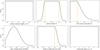 |
Fig. 3. Priors of NH, Γ, q, kT, R, and fscatter. The dashed orange lines point out the locations where the priors switch to different analytical expressions. See Table 2 for details. |
Informative priors were used for the parameters of the secondary components that are difficult to measure. The priors of fscatter, R and kT were taken from Ricci et al. (2017, see their Figs. 21, 30 and 31). In the case of fscatter , we set a Jeffreys prior with an upper limit of 10% and a lower limit of 0.01%. The prior on R is flat between 0 to 1.5 with a smooth Gaussian cut extending farther to 2.55. The prior on the temperature (kT) of the thermal component is written as a Gaussian prior centered at 0.5 keV with σ = 0.4 keV, and its intrinsic 2–10 keV luminosity (lumin) is constrained by a Jeffreys prior in the range from 1038 to 1041 erg s−1. The prior on the soft-excess strength q was derived from the distribution of the soft-excess strength from Boissay et al. (2016, see their Table A.2). It was fit with a flat distribution below 0.5 and a skew-normal distribution above, which was parameterized by  , where norm is the normal distribution, μ = 0.16, σ = 0.5, and α = 5.0. Its upper boundary was set to 1.8. The skew-normal distribution was implemented with the Python package scipy (Virtanen et al. 2020).
The XB model has just one free parameter, which is the normalization of the CXB, and we constrained it with a Jeffreys prior from 0.4 to 2.5 because it is a relative variation with respect to the average value we measure using ROSAT data (see Sect. 3.2). The priors on NXB continuum normalization parameters were obtained from an analysis of about 500 archival XMM-Newton extragalactic blank-field observations (Ghirardini et al. 2018). The multiplicative factor for the MOS NXB spectra was found to have an average value of 1.2 and a skewed distribution toward a higher value. We describe it as a Gaussian with positive skewness, which is skewnorm(x;μ,σ,α) as defined above, where μ = 1.08, σ = 0.27 and α = 9.14. In the case of the pn, the multiplicative factor is symmetric and centered on unity. We therefore describe it as a simple Gaussian, where μ = 1.04, σ = 0.06. We used Jeffreys priors for the multiplicative parameters of the fluorescence lines (fnxblines), which are bounded between 0.1 and 10.
3.4.2. Posterior sampling
The posterior was computed by applying the priors on the likelihood following Eq. (1). We sampled the posterior using MultiNest (Feroz & Hobson 2008; Feroz et al. 2009, 2019), which is an implementation of the nested-sampling algorithm (Skilling et al. 2004). The main advantages of MultiNest over more common sampling approaches such as a Markov chain Monte Carlo (MCMC) method are the capabilities to sample multimodal posteriors and compute the Bayesian evidence for model selection.
Our choice of extracting spectra from mosaics in fixed energy bins allowed us to implement the computation of the posterior much more efficiently, without using xspec. Because all objects have the same ARF and the same RMF (for a given instrument, pn or MOS), we can convolve the models once for all and create a large model grid, from which counts can be predicted using interpolations without additional convolution. We find an improvement in speed for our Python interpretation by a factor of 10 compared to using the BXA Python interface to MultiNest and xspec (Bayesian X-ray Analysis; Buchner et al. 2014).
We tabulate each spectral component used in our full model with the parameters described in Sect. 2.1. The details of the parameters of the grid are listed in Table 3. The model count rates for each set of parameters in the grid were computed using the xspec command fakeit with the proper ARF and RMF. The whole fitting process is implemented in Python using PyMultinest (Buchner et al. 2014), which provides a Python interface to the MultiNest library.
Intervals of spectral parameters.
3.4.3. Spectral analysis of NGC 788
We tested our spectral analysis method on the bright source NGC 788 (lower panel of Fig. 1) and compared the results with what was obtained using a standard fit to the full spectrum (see Sect. 2.2). Raw data (Obs. ID: 0601740201) were downloaded from the XMM-Newton Science Archive. Following the data analysis pipeline described in detail in Sect. 2.2 of Ghirardini et al. (2019), we used emchain and epchain of XMMSAS v13.5 to extract calibrated event files, and then applied the executables mos-filter and pn-filter to filter out time periods affected by soft-proton flares. Vignetting-corrected exposure maps were generated with eexpmap and count images were extracted from the three EPIC detectors in ten energy bins. The on-axis RMF and ARF files were generated with rmfgen and arfgen. The 10-bin source and background spectra of pn and MOS were then extracted from the images as described in Sect. 3.1. The radius of the source region is 40 arcsec and the inner and outer radii of the background region are 40 and 70 arcsec. Full-resolution spectra of pn and MOS were extracted following the standard SAS procedure to extract spectra of point-like sources using evselect. The same source and background regions were applied in both analysis.
We first fit the full spectra and the 10-bin spectra of both pn and MOS simultaneously in xspec using our full model. We added a second apec in the source model in this case to model residuals that are clearly detected in the spectra because of the high-S/N of this source. We were unable to generate our NXB models for the full-resolution spectra because they require binned images. We therefore modeled them using a power law plus two Gaussians centered on 1.6 and 8.0 keV, and then fit them to the 10-bin NXB. When we fit the full-resolution source+background spectra, parameters of this model were fixed to the best-fit values, and the same parameters of NXB as described in Sect. 3.2 were added to the fixed model and left free to vary. Figure 4 shows the simultaneous fit to the full pn and MOS spectra and to the 10-bin pn and MOS spectra. For clarity, only the full-resolution pn and the 10-bin MOS spectra are shown. The two spectra can be simultaneously fit with the same model and same parameter values, although the high-resolution spectrum shows complex residuals around the Fe Kα line.
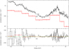 |
Fig. 4. Joint fitting of the spectra of NGC 788 extracted in two ways. The pn spectrum that is directly extracted in a standard way from event files, which has the full resolution, is shown in black, and the MOS spectrum extracted from aperture photometry in ten bins is shown in red. Together with the 10-bin pn spectrum and full-solution MOS spectrum, they are simultaneously fit to our source plus background model. |
To compare the results of the fitted parameters and their uncertainties, we used MultiNest to fit the two sets of spectra separately. For the full spectra, we used BXA to perform the spectral analysis in the xspec environment, while for the 10-bin spectra, we followed our method presented above and precomputed the model grid. The priors used for the parameters were the same in both cases (identical to Sect. 3.4.1). Marginalized posteriors of the two approaches are shown in Fig. 5. The two methods obtain consistent results. Although the PDFs of the full spectra are more narrowly distributed than those of the 10-bin ones, which is expected because of the small loss of information due to rebinning, our method using the 10-bin spectra is able to obtain similar measurements and even good constraints for parameters of secondary components, such as the reflection and thermal-emission components. Ricci et al. (2017) used a model (B3) very similar to our full model to fit the spectra of NGC 788. They found in general comparable results with our fitted values, for instance, log(NH)=23.77 ± 0.05, which agrees in general with our results. On the other hand, they find Γ = 1.64 ± 0.26, which is slightly lower than our fitted values. However, this difference can be explained by the fact that Γ has been determined using a fit that also makes use of Swift/BAT data and a free cutoff energy that is found to be around 70 keV. When the cutoff energy was fixed to 500 keV, Ricci et al. (2017) obtained Γ = 1.86 ± 0.08, which is consistent with our results.
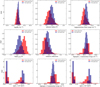 |
Fig. 5. Marginalized posteriors of the spectral parameters sampled using the 10-bin spectra (red) and the full spectra (purple). Error bars are the medians of the PDFs with 68% credible interval. |
This example shows that even at high S/N, the results of our spectral analysis method match those of the standard method, and the loss of information due to the binning of the spectra is minimum. The computation efficiency of our method is also demonstrated by this example: the sampling of the posterior using BXA for the full spectra takes more than 6 hours, but only takes about 20 minutes using our method. It is extremely expensive to use the full model, and it is much more difficult to apply it to very large samples.
3.5. Maximum-likelihood approach
For comparison, we present a spectral analysis method using the classical ML approach. In order to maintain high computation efficiency, we used our table models to calculate model spectra. Source plus background and background spectra extracted from the mosaics were fit together in order to preserve the Poisson statistics. The same likelihood function as shown in Sect. 3.3 was applied here.
To fit low-S/N data with a ML approach, there are two common practices. The first is to simply apply an absorbed power law for all the sources (Perola et al. 2004; Tajer et al. 2007). The second is to start with a simple power law, and then, depending on the quality of the fit, decide to apply a more complex model or not. The more complex model is selected depending on the characteristics of the spectra. However, because there is no direct estimate of the goodness-of-fit (GoF) for C-stat, it is not trivial how to assess when a more complex model is needed. Some authors bin the spectra such that each energy bin has more than 10–30 counts to approximate a χ2 distribution, for which a GoF exists, and a model selection can be made with an F-test (Mateos et al. 2005; Corral et al. 2011; Brightman & Nandra 2011). Others simply rely on a qualitative assessment, such as a visual inspection of the residues and of the deviations from the simple best fit (Tozzi et al. 2006; Shinozaki et al. 2006).
We propose here a statistically sound approach that can be applied automatically. We implement a ML approach as follows: we first define six different source models, using the components defined in Sect. 2.1, with different complexities as M1 to M6 listed in Table 4. The six models have 27, 26, 26, 25, 24, and 22 free parameters. We fit the spectra with all the models, and find the best-fit parameters for each of them. The optimization is performed using the MINUIT library (James & Roos 1975) via its iminuit Python interface. The best model for each source is then selected using the corrected Akaike information criterion (AICc; Cavanaugh 1997), which is the modified AIC for small sample sizes and calculated by AICc = AIC + (2k2 + 2k)/(n−k−1), where  .
.  is the maximum likelihood value of the model; k and n denote the number of parameters and the sample size, which is the number of data points of the spectra, respectively. We then simply select the model with the lowest AICc value.
Additive models used in the six models with different complexities in the ML approach.
4. Simulations
We compared the results of the Bayesian analysis we have described above with those obtained with the ML approach. For this purpose, we simulated a realistic sample of AGN and created representative source and background spectra. Finally we applied both our Bayesian spectral-analysis method and the classical ML spectral-analysis approach on them. We describe below the simulations and the results in detail.
4.1. Simulated sample
We first built a sample of 5000 AGN to a relatively deep depth, and created for each of them pn and MOS spectra with background. The exposure time was randomly drawn from a log-normal distribution 10t ks, with  , where 2 is the mean and 0.225 is the variance. Our full model (Sect. 2.1) was used to simulate the source spectra. Γ was drawn from a Gaussian distribution with mean μ = 1.95 and standard deviation σ = 0.15 (Nandra & Pounds 1994; Buchner et al. 2014). NH, F, q, kT, lumin, R, and fscatter were drawn from their priors described in Sect. 3.4.1. The galactic hydrogen column density was fixed at 1.74 × 1020 cm−2. The redshift was converted from the comoving distance, which was randomly drawn in the comoving volume up to redshift 4, assuming AGN are uniformly distributed in space. The cosmology we assumed is the WMAP9 ΛCDM: H0 = 69.3 km/s/Mpc, ΩΛ = 0.72, Ωm = 0.28, and σ8 = 0.82 (Hinshaw et al. 2013). To calculate the intrinsic rest-frame 2–10 keV luminosity (LX), we only considered the unabsorbed primary power law and reflection, as the other components contribute mostly below 2 keV, for example, soft excess, or are much smaller than the primary power law when there is no absorption, for example, scattering. Simulated objects were then selected so that LX follows the X-ray luminosity function (LXF) of Aird et al. (2015). We used the flexible double power-law model parameterized in the hard band.
XB was simulated based on the XB model defined in Sect. 3.2, and NXB was simulated using a random NXB spectrum of the XMM-COSMOS sample described in Paper II as a template. Background parameters were also randomly drawn from their priors. With the source and background spectra and the exposure time, we calculated the photon counts in the 2–7 keV band as well as the S/N, defined as  , where Ns is the total number of counts in the source region, Nb is that in the background region, and r is the ratio of the background and the source area. We applied a simple selection at S/N > 3 to reject undetectable source. The final count rate and S/N distributions of the simulated sample are shown in Fig. 6. We measured the fraction of selected sources after applying the S/N cut as a function of count rate, and fit it using the selection function presented in Sect. 3.3. We obtain the parameters a = 5.2 ± 0.9 and b = 3.42 ± 0.02. The fitted selection function is shown in Fig. 7.
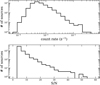 |
Fig. 6. Histograms of count rate (top) and S/N (bottom) of the simulated sample in the 2–7 keV band. |
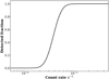 |
Fig. 7. Selection function of the simulated sample based on count rate (s−1) . |
Due to the strong selection effect for highly absorbed sources, there are not enough Compton-thick (CT; i.e., sources with NH ≥ 1.6 × 1024 cm−2) sources in the simulated sample above. To better compare the performance of different spectral fitting methods in the CT regime, we simulated another sample of 500 CT AGN by drawing NH between 1024 and 5 × 1024 cm−2, everything else being unchanged.
4.2. Results
We applied both our Bayesian method and the ML method on the simulated sample. For the ML approach, we find after the model selection that the majority of the sample (3590) prefers M3 (power law plus reflection), while 385, 22, 1022, 472, and 9 sources require M1, M2, M4, M5, and M6 respectively. Figure 8 shows the improvement of three estimators after the model selection. The first two are the Pearson-reduced  , which is the χ2 used for Poisson data with finite counts, and the C-stat divided by the number of d.o.f. These two estimators are not accurate enough for a model selection because they would be valid in the limit of a large number of counts or data points; we can nevertheless qualitatively see the improvement in the fit. All objects with
  or reduced C-stat higher than 3 obtain a better fit after model selection than the results with M1 alone, which shows that more complex models fit these spectra significantly better. The plot in the right panel of Fig. 8 shows the distribution of AICc, which is largely reduced after model selection. This shows that despite the low-to-moderate S/N, the spectra of most objects require not only an absorbed power law, but also a reflection component and sometimes a soft excess as well. On the other hand, models with high complexity (M5 and M6) are rarely required by the data, even though M6 is the correct model. By contrast, the Bayesian method does not require any selection.
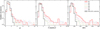 |
Fig. 8. Reduced |

We compare the results of the fitting of spectral parameters, especially the primary parameters, for example, NH, Γ and the rest-frame 2–10 keV intrinsic X-ray luminosity (LX). We show the results of ML with AICc model selection, as well as M1 alone, because M1 is usually applied to low-S/N data in the literature. The main difference between the ML and Bayesian analysis results is that the ML provides single values for these parameters, while Bayesian analyses provide posterior distributions. For a fair comparison, we therefore computed the two-dimensional histograms of the best-fit ML values versus the true input values for the ML measurements, while we stacked the PDFs for the Bayesian posteriors in each bin. Then we compared the resulting 2D histograms with the 2D stacked PDFs, as shown in Fig. 9.
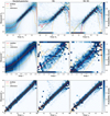 |
Fig. 9. Stacked probability density plots of NH, Γ, and LX obtained with the different fitting approaches. Left column: Bayesian method. Middle: ML method. Right: M1 model. The true values are binned to 30 bins. The red line shows the medians of the distribution in each bin, and the dashed orange lines are the 16% and 84% percentiles. The dashed green line shows the reference where the fitted value equals the true one. |
4.2.1. Hydrogen column density NH
The results of the fitting of NH are shown in the first row of Fig. 9. An obvious characteristic shared by both methods is that NH is very well constrained for non-CT absorbed sources, defined as NH between 1022 and 1024 cm−2, while it is poorly constrained for unabsorbed sources. This is mainly due to the loss of sensitivity of the soft X-ray spectrum to the change of NH when NH becomes too small. Although we are not able to provide a good estimate of the actual NH for unabsorbed sources, we can still say with high confidence that they are unabsorbed. In the CT regime, the increased noise and bias is due to the limited information present in the XMM-Newton spectra of these objects.
For non-CT absorbed sources, the results of the Bayesian method and ML with selection are comparable in terms of the average bias and dispersion, which are both very small. The measurements of ML using M1 alone, which is the simplest model, are also quite good, but NH is biased toward lower values. The reason is that M1 ignores soft excess, thermal emission, and the scattered component, which is compensated for by the smaller absorption of the fit. As shown in the middle left panel of Fig. 10, the Bayesian approach underestimates NH from 1022 to 1022.5 cm−2 while it overestimates it from 1022.5 to 1023.5 cm−2. The reason is that the likelihood changes very little for either very low values or for very high values of NH, therefore the posterior extends more to the lower or higher limit of NH. This systematic bias is small, however.
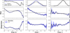 |
Fig. 10. Parent distributions of NH, Γ, and LX (from left to right). Top row: parent distributions of the main parameters (dashed blue) compared to those after selection (black). The parent distribution of LX is not shown because it was computed based on other spectral parameters and then selected by the XLF (see Sect. 4.1). Middle and bottom rows: average bias and dispersion with 1σ uncertainties (blue area) of the Bayesian method with respect to the true values. In each bin we randomly drew one value from each PDF and then computed the bias and dispersion, and this procedure was repeated for 1000 times to obtain the average bias and dispersion, together with their uncertainties. |
NH of CT sources is not well determined by any method. However, Fig. 9 shows that the median line of the stacked PDFs remains around 1024 cm−2, while many results of ML methods are highly biased to much lower values. This shows that our Bayesian method is able to constrain most of the CT sources to lie in the vicinity of the CT regime, while the ML methods quickly lose their constraining power of NH.
Although neither the ML nor the Bayesian methods are able to constrain NH very well, there are still significant differences in the results for unabsorbed sources. For ML with M1 alone, the vast majority of sources are accumulating at the lower boundary, and the others are randomly scattered up to about 1022.5 cm−2, which is caused by the fact that we ignored the secondary components. The average bias for ML with selection appears to be largely reduced, but this is just an average effect of two clusters of the fits, one hitting the lower boundary and the other accumulating around 1022cm−2. A few sources are also fit with very large NH up to 1024 cm−2. In reality, very few ML fits provide a correct value for NH when NH < 1022 cm−2. The reason is that more complex models are selected with our model selection approach, which introduces degeneracies between NH and the other parameters. By contrast, the stacked NH posterior given by the Bayesian analysis is mostly flat and concentrated below 1022 cm−2. This means that even though NH is not well constrained, the classification of the sources between the absorbed and unabsorbed categories is accurate. The loss of sensitivity of the data to NH blurs the posterior, but does not introduce a strong bias.
To show the different performances of the approaches on unabsorbed sources better, we plot the measured NH distributions of the unabsorbed subsample in Fig. 11. It is clear that both ML approaches fail at reproducing the expected NH distribution, which is flat. Very few sources with NH between 1020 to 1021 cm−2 are recovered by ML, and the false impression arises that this distribution is bimodal. On the other hand, our Bayesian method returns mostly flat PDFs in this range, which mostly follow the prior. However, even though the NH of individual sources is not well constrained, the PDFs still contain some information, for instance, the maximum allowed NH, unlike the ML results, for which a large fraction of sources hit the lower boundary of the allowed range. The method that we devised to infer the properties of the parent population from the output PDFs is presented in Paper II.
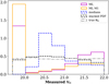 |
Fig. 11. Distributions of NH in the unabsorbed subsample (NH < 1022 cm−2). The result with the ML approach using AICc selection is shown by the solid magenta line, and the approach using M1 alone is shown by the solid orange line. The results with the Bayesian method using medians and stacked PDF are shown by the dashed blue and black lines, respectively. The gray line shows the parent distribution. |
4.2.2. Spectral index Γ
The results of the fitting of the photon index Γ using the two methods are shown in the second row of Fig. 9. There are clearly significant biases in the ML fit, where the fitted photon indices for many sources hit the fit boundaries at Γ = 1.4 and 2.6, and the formal error on Γ is very small and largely underestimated. In addition, the photon indices obtained with ML with model selection show a constant bias toward larger Γ, while the fits for ML with M1 alone show a constant negative bias. The negative bias when M1 alone is applied is mostly caused by the presence of the reflection component, which is ignored by the simplest model, while the positive bias of the other is due to the overfitting of secondary components, for instance, fitting the reflection parameter to the maximum value (see Sect. 4.2.4).
By contrast, the Bayesian method shows a more reasonable systematic bias and very few outliers. In the range of 1.8 to 2.2 where most of the photon indices are expected (Nandra & Pounds 1994; Buchner et al. 2014), the Bayesian method has a very small bias and dispersion, as shown in the middle column of Fig. 10. The bias becomes larger when Γ approaches the boundaries, mainly because the edges of the prior (see Sect. 3.4.1) cut the low- or high-Γ extension of the posteriors. In addition, only a few sources lie in this range in our simulation because we drew our true Γ from a Gaussian distribution centered at 1.95 (see Sect. 4.1). The results can therefore be affected by small-number statistics. These values are not really expected in reality, however (Buchner et al. 2014). If the true Γ really follows the distribution of Buchner et al. (2014), our method would be able to recover Γ for the vast majority of the objects with little bias and dispersion. The average bias of the ML methods is very misleading. The average bias of the ML methods with model selection for sources with true Γ around 2 would indeed be very small, even though most of the measurements are very poor, as shown in Fig. 9, and they are randomly scattered to the two boundaries, so that the average value happens to be very close to the true value. The dispersion is also meaningless in these cases because it mostly depends on where the boundaries of the fits are defined.
Because NH strongly affects the measurement of Γ, we divided our simulated sample into absorbed and unabsorbed subsamples with the boundary set at NH = 1022 cm−2. We plot the results of ML with model selection and our Bayesian method in Fig. 12. The constraints on Γ with both methods are much better for unabsorbed sources than for absorbed sources, as expected. However, there are still some catastrophic failures of ML even in the unabsorbed subsample, while the Bayesian method gives smooth stacked PDFs with very small bias and dispersion. For the absorbed sub-sample, both approaches are unable to measure Γ correctly, but unlike our Bayesian method, which gives smooth PDFs, ML severely biases the measurements of Γ to extreme values, often reaching the fit boundaries. Again, the median of ML is misleading because very few measurements of Γ using ML are meaningful (i.e., do not hit the fit boundaries). As also shown in Fig. 13, more than 40% of the absorbed sources are fit by ML with Γ around 1.4 or 2.6. By contrast, in the Bayesian approach, the medians of the Γ posteriors roughly recover a correct Γ distribution, which in our case is a Gaussian around 1.95 (see Sect. 4.1). The posteriors are close to the flat prior from 1.5 to 2.5, however, which can be seen from the stacked PDF. With a flat posterior the median of the posterior is equal to the central value of the range, which is arbitrary, and in fact, neither the medians nor the stacked PDF provides a correct reconstruction of the parent population; we address this point in Paper II. This also shows that when there is little information in the data to constrain a parameter, ML is very unstable and tends to adopt highly biased values, while in the Bayesian approach, the values of the parameter remain constrained by the prior to a range of acceptable values according to our previous knowledge.
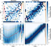 |
Fig. 12. Measured Γ with ML with AICc model selection (top row) and stacked posteriors (bottom row) against the true value for different subsamples: NH > 1022 cm2 (absorbed, left column), NH ≤ 1022 cm2 (unabsorbed, right column). The red line shows the medians of the distribution in each bin, and the dashed orange lines are the 16% and 84% percentiles. The dashed green line shows the reference where the fitted value equals the true one. |
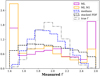 |
Fig. 13. Distributions of Γ in the absorbed subsample (NH > 1022 cm−2). The result with the ML approach using the AICc selection is shown by the solid magenta line, and the result using M1 alone is shown by the solid orange line. The results with the Bayesian method using medians and stacked PDF are shown by the dashed blue and black lines, respectively. The gray dot-dashed line shows the parent distribution. |
4.2.3. X-ray luminosity LX
We compared the intrinsic 2–10 keV LX recovered with the different fitting approaches with the true LX. In the case of the ML methods, LX was computed using the best-fit parameters. In the Bayesian analysis, a PDF of LX was obtained by randomly drawing many sets of spectral parameters from the corresponding posteriors and then computing LX for each of them.
Figure 9 shows that all methods are able to constrain LX well, but there are still significant differences in their performances. First of all, for some sources the ML method with model selection biases LX to much higher values, some as high as 1046 erg s−1 , while the true LX is only about 1043 erg s−1. Even though these outliers only amount to about 3% of the total sample, the biased measurements of LX might affect the computation of the luminosity function at the bright end strongly because there are intrinsically few very luminous sources in the sample. This bias is mostly due to the degeneracy between unabsorbed power law and absorbed power law plus scattering: if the source is intrinsically faint, we can fit it with a source with a much higher luminous, but highly absorbed, together with a scattering component. The scattering, although its luminosity is lower than 10% of that of the primary power law, is still enough to compensate for the soft X-ray part of the spectrum. When the ML method is used with M1 alone, it appears to be able to measure LX with a small bias and only a few outliers, even though its measurements of NH and Γ are often strongly biased. However, this is simply because in the 2–10 keV band, where NH has a smaller impact, a simple power law with harder photon index can be still a good fit of a spectrum, which is intrinsically a softer power law plus reflection.
By contrast, the Bayesian approach is able to constrain LX throughout most of the range, without obvious bias and dispersion. The degeneracy observed with the ML method is largely removed by the use of strong priors on secondary components. This shows that, on one hand, the measurement of the hard-band LX is mostly robust, even when the column densities and photon indices are not measured accurately; on the other hand, the Bayesian method is still more robust than the ML one, with or without model selection.
4.2.4. Secondary parameters
The typical S/N in our simulated sample does not allow us to constrain the secondary spectral parameters such as reflection and soft excess. Figure 14 shows the corresponding posteriors, which simply follow their priors, meaning that we do not gain any information from the data for these parameters of most sources. We also show the ML measurements of secondary parameters in Fig. 14, except for those of the thermal component because they are most often ignored in the ML analysis (see Sect. 3.5).
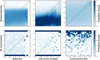 |
Fig. 14. Two-dimensional stacked posteriors of secondary spectral parameters, the reflection R, soft excess strength q, and scattering fraction fscatter, which are shown from left to right. Top row: results of the Bayesian method, and the bottom row shows those of the ML method. When an ML model does not include one of these secondary components, the corresponding parameter is fixed to 0. The dashed green line shows the reference where the fitted value equals the true one. |
Although both methods are unable to constrain these parameters, there are still significant differences in the results. The ML approach results in extreme values for most of the sources. For example, R is mostly fit with either the maximum value 2.5 or 0 (ignored), even though the values at the boundaries are unlikely to exist in reality. These results give us incorrect information on the parameters and bias the measurements of the other parameters. On the other hand, the stacked PDFs of the Bayesian method are smoothly distributed in the areas that are constrained by the priors. This clearly shows that the data are not able to constrain these parameters, but their errors are correctly propagated into the posteriors of the main parameters.
5. Discussion
5.1. Bayesian versus ML approaches
The ML approach shares some common features with the Bayesian approach in the sense that they both use the same likelihood function as an essential ingredient to estimate their parameters. However, there are also fundamental differences between the two methods that strongly impact the results when they are applied them to a large number of AGN X-ray spectra with low to moderate data quality, as is typical of surveys.
The first difference is that the ML approach does not allow the use of priors to place constraints on secondary parameters, so that fitting complex models to data with a low S/N results in very unstable ML parameters. As we have shown in Figs. 13 and 14, when the data contain little information on parameters such as R, the value recovered by the ML approach tends to hit the boundaries of the allowed range. When this approach is applied blindly, it might naively be thought that the parameters are well constrained. Because some of the parameters of the model are correlated, these highly biased measurements can affect those of some of the parameters of interest (NH, Γ, LX).
The ML M1 and ML methods that we have presented mimic the approach followed in most of the literature when Bayesian methods are not used. The first approach, ML M1, ignores secondary components, which can bias some spectra that appear very simple but are actually complex (see Sect. 2.4), due to the degeneracy between the primary and secondary parameters. The application to the simulated sample shows that ML M1 biases NH toward lower values and quickly loses its constraining power when the absorption is lower than 1022 cm−2 (see Fig. 9). It also constantly biases Γ to harder values, as shown in Fig. 10. Therefore the simple model is not able to recover sensible parameters even though the fit appears reasonable, so that more complex models are required.
We tested an objective and automatic model selection procedure based on six models with increasing complexity. Model selection was performed using the AICc estimator. Somewhat surprisingly, the simplest model is always excluded. Instead, moderately complex models, most often with reflection (M3), but sometimes with soft excess (M2), are preferred. Buchner et al. (2014) also found that reflection is usually needed (see details in Sect. 5.2). The overall improvement of the fits is demonstrated in Fig. 8 with approximate estimators of GoF that are largely reduced after model selection. NH is relatively well measured for non-CT absorbed sources with smaller bias than when M1 is used alone. However, the measured NH for unabsorbed sources are still unusable, as shown in Fig. 11, and the ML method with model selection is still unable to provide a reliable estimate of the photon index Γ, as most of the fitted values hit the upper and lower boundaries of the allowed range (see Figs. 9 and 13). While all methods (including M1) can accurately retrieve the intrinsic luminosity of the source, when we account for about 3% of the sources in our sample, there is a small cluster of sources with highly biased LX, which is probably due to the strong degeneracy with some secondary parameters (see Fig. 14). Therefore it is still not sufficient to apply ML with more complex models to constrain the main spectral parameters without obvious bias.
By contrast, our Bayesian approach is able to apply the full model (M6) to all the sources and still obtain mostly unbiased fits for the main parameters of interest, namely NH, Γ , and LX. The main reason is that the Bayesian approach uses informative priors to constrain secondary parameters, avoiding the impact of secondary components being fitted with unrealistically extreme values, as discussed above. In the end, it marginalizes over the secondary parameters that are unconstrained, as well as over the nuisance parameters of the background models, to obtain the PDFs of the main parameters. This propagates the uncertainties correctly. Another reason is that our Bayesian approach samples the entire parameter space with MultiNest, while ML approaches are prone to ending up in local maxima, especially when the models are very complex and the parameter space is highly dimensional.
Another main difference is that the Bayesian approach produces PDFs that contain the full posterior probability information, while ML only provides point estimates. In some case, the PDFs may still be biased, for instance, those of NH for unabsorbed sources. However, even when they are biased, the PDFs practically always cover the true values, so that it can still help to reproduce the parent parameter distributions, which is the main goal of this analysis. In contrast, the ML approach leads to many catastrophic failures, in which case it is impossible to reconstruct the parent population, for example, in the two cases shown in Figs. 11 and 13. In Paper II we propose a method for recovering the parent distribution in the presence of biased PDFs.
5.2. Comparison with other Bayesian methods
Three groups have already pioneered Bayesian analysis of AGN X-ray spectra: Buchner et al. (2014), Fotopoulou et al. (2016), and Ruiz et al. (2021). A common feature of the spectral analysis methods in these works, as well as ours, is that a nested-sampling algorithm such as MultiNest is applied to sample the full parameter space.
Fotopoulou et al. (2016) adopted a similar but much simpler approach to ours to fit the XXL-1000-AGN sample. The background spectra and source plus background were fit simultaneously in order to preserve the Poisson statistics. The background spectra were modeled with the same XB model as we used. However, the NXB was modeled with a combination of several emission lines and continuum components, which are phenomenologically represented by blackbodies and/or power laws, while we used the FWC data as described in Sect. 3.2.2. The most important difference between our method and that of Fotopoulou et al. (2016) is that they adopted a simple absorbed power-law model for all the sources. Even though noninformative priors were used for Γ and NH, ignoring secondary components such as reflection and soft excess could bias the PDFs. For example, we have shown in Sect. 2.4 that even when the data appear to be simple, the spectrum may be intrinsically complex.
Buchner et al. (2014) analyzed the X-ray spectra of about 350 AGN in the four Ms Chandra Deep Field South using a Bayesian method to select among ten physically motivated models with different complexities, from a simple power law to a complex model including secondary components. The components considered in the models include the primary power law, absorption, reflection, and scattering. Soft excess was neglected because it lies outside of the observed energy range of most of the sources because of the redshift. Background and source plus background spectra were fit separately, with the background fit first using a Gaussian mixture model and then fixed in the fitting of the source plus background spectra. This is a common approach to model background in general, but our NXB model represents the most advanced modeling of the XMM background (Ghirardini et al. 2018). A Jeffreys prior was also applied to NH, but a strong Gaussian prior with a mean 1.95 and a standard deviation 0.15 was adopted for Γ. In general, our simulations have shown that measuring Γ is difficult, especially for absorbed sources, thus they only marginalized over it. In addition, noninformative priors were applied on secondary components, while we used informative priors obtained from deep surveys to constrain the complex models. Another difference is that we included the selection function into our likelihood function, in order to exclude undetectable fits in the source detection band.
A further difference between Buchner et al. (2014) and our work is that they employed model selection among many models with different complexities, while we consistently used the most complex model for all the sources. However, their overall best model after model selection ends up with powerlaw+torus+pexmon+scattering, where powerlaw is the primary emission, torus is the absorber, pexmon is the reflection, and the last item is the scattering. This is also a complex model and very similar to ours, especially considering that soft excess and thermal emission do not apply to their mostly high-z sources. For the low-z universe, however, soft excess and thermal emission are present in the soft X-ray band. General criteria are used in Buchner et al. (2014) for model selection, such as the Bayes factor and BIC and AIC values. We propose in this paper a generalization that is valid for sources at all redshifts, more advanced NXB background modeling for XMM-Newton, and, most importantly, the use of informative priors for the secondary components, as well as a complete likelihood that takes the selection function into account. Similar approaches were used in Liu et al. (2016, 2022) to analyze the point-like X-ray sources in the northern field of the XMM-XXL survey and those in the eROSITA final equatorial-depth survey (eFEDS), respectively, except that Liu et al. (2016) applied the best model of Buchner et al. (2014) for all the sources, while Liu et al. (2022) applied simpler models, including the primary power law, with NH or Γ fixed in some cases, and sometimes a soft-excess component.
Ruiz et al. (2021) also used a similar approach to Buchner et al. (2014) to analyze about 22’700 sources in the 3XMM catalogue to search for obscured sources. Four phenomenological models were considered, including an absorbed power-law model, an absorbed thermal model, an absorbed thermal plus power-law model, and an absorbed double power-law model. Other secondary components, such as reflection and soft excess, were neglected. Similarly to Buchner et al. (2014), noninformative priors were applied on secondary components, which makes it more difficult to constrain complex models. The best model was selected using the Kolmogorov-Smirnov (KS) statistics and the corresponding p-value, and the evidence provided by MultiNest for each model. As a result, the simple absorbed power-law model was accepted or preferred for most the sample (90%). Another difference is that Ruiz et al. (2021) used the W statistics in xspec to take the Poisson background into account, but this is not exact and will lead to biases for weak sources and small numbers of counts in the background spectrum (see Appendix B of the Xspec User Guide6). In our work, we modeled the source plus background and background simultaneously, fully preserving the Poisson statistics.
A final difference in the different approaches is that the whole fitting process is done outside of the usual X-ray spectral fitting softwares such as xspec. All spectra are binned in the same way and extracted in a way to have a single response (for each instrument), and models are preconvolved with the response once for all in large model matrices. This results in a large gain in the computing efficiency of the spectral analysis.
5.3. Effect of the redshift on NH
The constraint on NH is highly dependent on the redshift, as shown in Fig. 15. We divided the total sample into four redshift bins: [0, 0.6], [0.6, 1.0], [1.0, 1.5], and [1.5, 4], so that the number of sources in each bin is roughly the same. In the first redshift bin, there is a very clear transition point around 1021.5 cm−2, above which the measurements of NH are very well constrained, while the measurements fail below it and the posterior becomes uniformly redistributed, but still remaining in the unabsorbed region. As redshift increases, this transition point moves towards higher absorption. Despite the increased noise in the plot of the highest redshift bin due to the decreased S/N on average, a transition point can be clearly identified above 1022 cm−2. The reason is that the information for NH ∼ 1022 cm−2 is concentrated below about 2 keV in the rest frame, and that the redshift moves the informative part of the spectrum to lower energies outside of the considered spectral range.
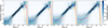 |
Fig. 15. Two-dimensional stacked PDFs of NH of subsamples in different redshift bins: [0,0.6], [0.6,1.0], [1.0,1.5], and [1.5,4], from left to right. The red line shows the medians of the distribution in each bin, and the dashed orange lines are the 16% and 84% percentiles. The dashed green line shows the reference where the fitted value equals the true one. |
There is also a similar effect for CT sources. In the first redshift bin, the uncertainties in NH increase very rapidly above 1024 cm−2. However, at higher redshifts, the uncertainty in the NH of CT sources becomes clearly smaller, with more probability constrained to the CT regime and its vicinity. This can be also naturally explained by the fact that the absorption feature and Compton hump are redshifted to lower energies, which gives the soft X-ray spectrum stronger constraining power over NH.
5.4. Effect of uncertainties in the redshift
The redshift is obviously also an important parameter in the fitting of AGN X-ray spectra in large surveys. Because it is time consuming to obtain spectroscopic redshifts (spec-z) for each source, photometric redshifts (photo-z) must be used for some of the sources. Many photo-z codes today produce probability distribution function (PDZ) using template fitting (Benítez 2000) or machine learning (Carrasco Kind & Brunner 2013), as well as many other subsequent works.
In principle, the PDZs can be used as a prior on a redshift parameter that we can fit using our approach without any modification, and in fact, in the model presented above, the redshift is already a free model parameter with a very strong prior. In the end, the photo-z is marginalized to propagate its uncertainty into the posterior distribution of the main parameters, similarly to the secondary and nuisance parameters. However, considering that our model is already very complicated and the fit of soft X-ray spectrum is quite sensitive to redshift, especially for low-S/N data, in this paper we assumed that a spec-z, or an excellent quality photo-z, is available, such that the prior on the redshift is effectively a Dirac distribution. In addition, photometric redshifts are subject to catastrophic failure, such that the PDZs do not necessarily represent the true posterior probabilities of the redshift. Thus we consider that including the full PDZs, while technically perfectly feasible within our analysis framework, would uncover problems that are not directly related to the analysis of X-ray data, and thus are beyond the scope of this work.
6. Conclusion
We developed a novel Bayesian method using nested sampling to automatically fit a large number of AGN X-ray spectra at low-S/N level. A single physically motivated model was adopted for all the sources, including the primary power law, soft excess, reflection, scattering, and emission from thermal plasma. We applied noninformative priors for the most relevant spectral parameters, for instance, NH and Γ, aiming at constraining their distributions from the data, and informative priors derived from deep observations on the other parameters that are difficult to constrain with low-S/N data, to properly propagate their uncertainties by marginalizing over them. We implemented the survey selection function directly into our Bayesian model by modifying the likelihood to discard sources whose count rates in the detection band were below the detection threshold. This complete likelihood was used to penalize undetectable solutions due to the difference between the source detection band and the spectral fitting band. We modeled source and background spectra simultaneously to preserve Poisson statistics, and the NXB model was derived with filter-wheel-closed data. The spectra were extracted from aperture photometry with consistent energy binning, which allowed us to tabulate xspec models by convolving the theoretical models with the constant redistribution matrix, largely speeding up both the spectral extraction and model fitting.
We tested our method on a realistic sample of 5000 simulated spectra (plus about 500 CT objects), most of which have low S/N (3–5). Based on the results in Sect. 4, our Bayesian method is able to constrain the main spectral parameters, namely NH and Γ, and to recover the intrinsic X-ray luminosity even at low-S/N level. The NHs of absorbed sources are accurately recovered, and for unabsorbed sources, we obtain a correct upper limit of NH. Γ was fit with relatively large uncertainties for absorbed sources, but for unabsorbed sources, we were able to obtain a good constraint. The intrinsic X-ray luminosity is very well recovered for the whole sample, which is important for studying the demographics of AGN population. On the other hand, parameters of secondary components such as reflection and soft excess are poorly constrained, but this is expected. Applying informative priors allowed us to marginalize over the range of acceptable model parameters and to propagate the uncertainties to the parameters of interest.
The advantages of our new approach of AGN X-ray spectral fitting can be summarized as follows:
-
Consistent physical model: A comprehensive physics-driven model was applied to all sources without model selection and regardless of the S/N. It overcomes the bias introduced by selecting models based on the apparent model complexity.
-
Background modeling: Source and background spectra were modeled simultaneously to preserve the Poisson statistics. The background was modeled using a theoretical model for XB and normalized filter-wheel-closed data for NXB.
-
Automatic and fast analysis: The whole spectral analysis process is fully automatic from spectral extraction to parameter estimation, and it is computationally very efficient based on a pure Python code that bypasses the need to use software such as xspec. This is a key requirement of large X-ray surveys.
-
Bayesian parameter estimation: The Bayesian analysis using nested sampling allowed us to fully explore the high dimensional parameter space and to obtain the full posterior distribution of each parameter. The uncertainties of secondary and nuisance parameters were correctly taken into account by marginalizing over them, which gives us a mostly unbiased estimation of parameters of interest, such as NH, Γ and LX.
In Paper II we expand the Bayesian spectral analysis to determine the properties of the parent population using a fully Bayesian approach. We take full advantage of the posteriors of the parameters derived using the method proposed here.
This object even requires two apec at different temperatures because its S/N is very high.
In this paper, R is the physical property and is always positive, but −R is passed to the xspec model to ignore the direct emission in pexmon.
Acknowledgments
L.G. acknowledges partial support from the Swiss National Science Foundation.
References
- Aird, J., Coil, A. L., Georgakakis, A., et al. 2015, MNRAS, 451, 1892 [Google Scholar]
- Akaike, H. 1974, IEEE Trans. Autom. Control, 19, 716 [Google Scholar]
- Ananna, T. T., Treister, E., Urry, C. M., et al. 2019, ApJ, 871, 240 [Google Scholar]
- Arnaud, K. A. 1996, ASP Conf. Ser., 101, 17 [Google Scholar]
- Arnaud, K. A., Branduardi-Raymont, G., Culhane, J. L., et al. 1985, MNRAS, 217, 105 [NASA ADS] [CrossRef] [Google Scholar]
- Avni, Y., & Tananbaum, H. 1986, ApJ, 305, 83 [Google Scholar]
- Baloković, M., Harrison, F. A., Madejski, G., et al. 2020, ApJ, 905, 41 [Google Scholar]
- Benítez, N. 2000, ApJ, 536, 571 [Google Scholar]
- Bianchi, S., Guainazzi, M., & Chiaberge, M. 2006, A&A, 448, 499 [NASA ADS] [CrossRef] [EDP Sciences] [Google Scholar]
- Bianchi, S., Guainazzi, M., Matt, G., Fonseca Bonilla, N., & Ponti, G. 2009, A&A, 495, 421 [NASA ADS] [CrossRef] [EDP Sciences] [Google Scholar]
- Blandford, R. D., Netzer, H., Woltjer, L., Courvoisier, T. J. L., & Mayor, M. 1990, Active Galactic Nuclei (Springer) [CrossRef] [Google Scholar]
- Boissay, R., Paltani, S., Ponti, G., et al. 2014, A&A, 567, A44 [NASA ADS] [CrossRef] [EDP Sciences] [Google Scholar]
- Boissay, R., Ricci, C., & Paltani, S. 2016, A&A, 588, A70 [NASA ADS] [CrossRef] [EDP Sciences] [Google Scholar]
- Brandt, W. N., Laor, A., & Wills, B. J. 2000, ApJ, 528, 637 [CrossRef] [Google Scholar]
- Brightman, M., & Nandra, K. 2011, MNRAS, 413, 1206 [NASA ADS] [CrossRef] [Google Scholar]
- Buchner, J., Georgakakis, A., Nandra, K., et al. 2014, A&A, 564, A125 [NASA ADS] [CrossRef] [EDP Sciences] [Google Scholar]
- Buchner, J., Georgakakis, A., Nandra, K., et al. 2015, ApJ, 802, 89 [Google Scholar]
- Burlon, D., Ajello, M., Greiner, J., et al. 2011, ApJ, 728, 58 [Google Scholar]
- Carrasco Kind, M., & Brunner, R. J. 2013, MNRAS, 432, 1483 [Google Scholar]
- Cash, W. 1979, ApJ, 228, 939 [Google Scholar]
- Cavanaugh, J. E. 1997, Stat. Probab. Lett., 33, 201 [CrossRef] [Google Scholar]
- Chiappetti, L., Fotopoulou, S., Lidman, C., et al. 2018, A&A, 620, A12 [NASA ADS] [CrossRef] [EDP Sciences] [Google Scholar]
- Corral, A., Della Ceca, R., Caccianiga, A., et al. 2011, A&A, 530, A42 [NASA ADS] [CrossRef] [EDP Sciences] [Google Scholar]
- Crummy, J., Fabian, A. C., Gallo, L., & Ross, R. R. 2006, MNRAS, 365, 1067 [Google Scholar]
- De Luca, A., & Molendi, S. 2004, A&A, 419, 837 [NASA ADS] [CrossRef] [EDP Sciences] [Google Scholar]
- Done, C., Davis, S. W., Jin, C., Blaes, O., & Ward, M. 2012, MNRAS, 420, 1848 [Google Scholar]
- Fabian, A. C. 2012, ARA&A, 50, 455 [Google Scholar]
- Fabian, A. C., Zoghbi, A., Ross, R. R., et al. 2009, Nature, 459, 540 [Google Scholar]
- Feroz, F., & Hobson, M. P. 2008, MNRAS, 384, 449 [NASA ADS] [CrossRef] [Google Scholar]
- Feroz, F., Hobson, M. P., & Bridges, M. 2009, MNRAS, 398, 1601 [NASA ADS] [CrossRef] [Google Scholar]
- Feroz, F., Hobson, M. P., Cameron, E., & Pettitt, A. N. 2019, Open J. Astrophys., 2, 10 [Google Scholar]
- Ferrarese, L., & Merritt, D. 2000, ApJ, 539, L9 [Google Scholar]
- Fotopoulou, S., Pacaud, F., Paltani, S., et al. 2016, A&A, 592, A5 [NASA ADS] [CrossRef] [EDP Sciences] [Google Scholar]
- Ge, L., Paltani, S., & Eckert, D. 2022, A&A, 667, A153 (Paper II) [NASA ADS] [CrossRef] [EDP Sciences] [Google Scholar]
- Gebhardt, K., Bender, R., Bower, G., et al. 2000, ApJ, 539, L13 [Google Scholar]
- Ghirardini, V., Ettori, S., Eckert, D., et al. 2018, A&A, 614, A7 [NASA ADS] [CrossRef] [EDP Sciences] [Google Scholar]
- Ghirardini, V., Eckert, D., Ettori, S., et al. 2019, A&A, 621, A41 [NASA ADS] [CrossRef] [EDP Sciences] [Google Scholar]
- Gibson, R. R., Brandt, W. N., & Schneider, D. P. 2008, ApJ, 685, 773 [NASA ADS] [CrossRef] [Google Scholar]
- Guainazzi, M., & Bianchi, S. 2007, MNRAS, 374, 1290 [Google Scholar]
- HI4PI Collaboration (Ben Bekhti, N., et al.) 2016, A&A, 594, A116 [NASA ADS] [CrossRef] [EDP Sciences] [Google Scholar]
- Hickox, R. C., & Alexander, D. M. 2018, ARA&A, 56, 625 [Google Scholar]
- Hinshaw, G., Larson, D., Komatsu, E., et al. 2013, ApJS, 208, 19 [Google Scholar]
- Hopkins, P. F., Somerville, R. S., Hernquist, L., et al. 2006, ApJ, 652, 864 [NASA ADS] [CrossRef] [Google Scholar]
- Iwasawa, K., Sanders, D. B., Teng, S. H., et al. 2011, A&A, 529, A106 [NASA ADS] [CrossRef] [EDP Sciences] [Google Scholar]
- James, F., & Roos, M. 1975, Comput. Phys. Commun., 10, 343 [Google Scholar]
- Jansen, F., Lumb, D., Altieri, B., et al. 2001, A&A, 365, L1 [NASA ADS] [CrossRef] [EDP Sciences] [Google Scholar]
- Kelly, B. C. 2007, ApJ, 665, 1489 [Google Scholar]
- Kolodzig, A., Gilfanov, M., Sunyaev, R., Sazonov, S., & Brusa, M. 2013, A&A, 558, A89 [NASA ADS] [CrossRef] [EDP Sciences] [Google Scholar]
- Kormendy, J., & Ho, L. C. 2013, ARA&A, 51, 511 [Google Scholar]
- Krolik, J. H. 1999, Active Galactic nuclei : from the Central Black Hole to the Galactic Environment (American Journal of Physics) , 68, 489 [Google Scholar]
- Lanzuisi, G., Gilli, R., Cappi, M., et al. 2019, ApJ, 875, L20 [Google Scholar]
- Lehmer, B. D., Xue, Y. Q., Brandt, W. N., et al. 2012, ApJ, 752, 46 [NASA ADS] [CrossRef] [Google Scholar]
- Liu, T., Buchner, J., Nandra, K., et al. 2022, A&A, 661, A5 [NASA ADS] [CrossRef] [EDP Sciences] [Google Scholar]
- Liu, Z., Merloni, A., Georgakakis, A., et al. 2016, MNRAS, 459, 1602 [Google Scholar]
- Maccacaro, T., Gioia, I. M., Wolter, A., Zamorani, G., & Stocke, J. T. 1988, ApJ, 326, 680 [NASA ADS] [CrossRef] [Google Scholar]
- Magorrian, J., Tremaine, S., Richstone, D., et al. 1998, AJ, 115, 2285 [Google Scholar]
- Mateos, S., Barcons, X., Carrera, F. J., et al. 2005, A&A, 433, 855 [NASA ADS] [CrossRef] [EDP Sciences] [Google Scholar]
- McCammon, D., Almy, R., Apodaca, E., et al. 2002, ApJ, 576, 188 [NASA ADS] [CrossRef] [Google Scholar]
- Mehdipour, M., Branduardi-Raymont, G., Kaastra, J. S., et al. 2011, A&A, 534, A39 [NASA ADS] [CrossRef] [EDP Sciences] [Google Scholar]
- Merloni, A., Predehl, P., Becker, W., et al. 2012, ArXiv e-prints [arXiv:1209.3114] [Google Scholar]
- Moretti, A., Campana, S., Lazzati, D., & Tagliaferri, G. 2003, ApJ, 588, 696 [NASA ADS] [CrossRef] [Google Scholar]
- Nandra, K., & Pounds, K. A. 1994, MNRAS, 268, 405 [Google Scholar]
- Nandra, K., O’Neill, P. M., George, I. M., & Reeves, J. N. 2007, MNRAS, 382, 194 [NASA ADS] [CrossRef] [Google Scholar]
- Perola, G. C., Puccetti, S., Fiore, F., et al. 2004, A&A, 421, 491 [NASA ADS] [CrossRef] [EDP Sciences] [Google Scholar]
- Piconcelli, E., Jimenez-Bailón, E., Guainazzi, M., et al. 2005, A&A, 432, 15 [NASA ADS] [CrossRef] [EDP Sciences] [Google Scholar]
- Pierre, M., Pacaud, F., Adami, C., et al. 2016, A&A, 592, A1 [NASA ADS] [CrossRef] [EDP Sciences] [Google Scholar]
- Pounds, K. A., Nandra, K., Stewart, G. C., George, I. M., & Fabian, A. C. 1990, Nature, 344, 132 [NASA ADS] [CrossRef] [Google Scholar]
- Ricci, C., Ueda, Y., Koss, M. J., et al. 2015, ApJ, 815, L13 [Google Scholar]
- Ricci, C., Trakhtenbrot, B., Koss, M. J., et al. 2017, ApJS, 233, 17 [Google Scholar]
- Ruiz, A., Georgantopoulos, I., & Corral, A. 2021, A&A, 645, A74 [NASA ADS] [CrossRef] [EDP Sciences] [Google Scholar]
- Sabol, E. J., & Snowden, S. L. 2019, sxrbg: ROSAT X-Ray Background Tool, Astrophysics Source Code Library [ascl:1904.001] [Google Scholar]
- Schwarz, G. 1978, Ann. Stat., 6, 461 [Google Scholar]
- Scott, A. E., Stewart, G. C., & Mateos, S. 2012, MNRAS, 423, 2633 [NASA ADS] [CrossRef] [Google Scholar]
- Shinozaki, K., Miyaji, T., Ishisaki, Y., Ueda, Y., & Ogasaka, Y. 2006, AJ, 131, 2843 [NASA ADS] [CrossRef] [Google Scholar]
- Silverman, J. D., Green, P. J., Barkhouse, W. A., et al. 2008, ApJ, 679, 118 [NASA ADS] [CrossRef] [Google Scholar]
- Singh, K. P., Garmire, G. P., & Nousek, J. 1985, ApJ, 297, 633 [NASA ADS] [CrossRef] [Google Scholar]
- Skilling, J. 2004, AIP, Conf. Ser., 735, 395 [NASA ADS] [CrossRef] [Google Scholar]
- Tajer, M., Polletta, M., Chiappetti, L., et al. 2007, A&A, 467, 73 [NASA ADS] [CrossRef] [EDP Sciences] [Google Scholar]
- Tozzi, P., Gilli, R., Mainieri, V., et al. 2006, A&A, 451, 457 [NASA ADS] [CrossRef] [EDP Sciences] [Google Scholar]
- Ueda, Y., Eguchi, S., Terashima, Y., et al. 2007, ApJ, 664, L79 [Google Scholar]
- Ueda, Y., Akiyama, M., Hasinger, G., Miyaji, T., & Watson, M. G. 2014, ApJ, 786, 104 [Google Scholar]
- Virtanen, P., Gommers, R., Oliphant, T. E., et al. 2020, Nat. Methods, 17, 261 [Google Scholar]
- Wilms, J., Allen, A., & McCray, R. 2000, ApJ, 542, 914 [Google Scholar]
- Zdziarski, A. A., Johnson, W. N., Done, C., Smith, D., & McNaron-Brown, K. 1995, ApJ, 438, L63 [NASA ADS] [CrossRef] [Google Scholar]
- Zdziarski, A. A., Johnson, W. N., & Magdziarz, P. 1996, MNRAS, 283, 193 [NASA ADS] [CrossRef] [Google Scholar]
All Tables
Additive models used in the six models with different complexities in the ML approach.
All Figures
|
Fig. 1. Unfolded energy spectra (eufs) of two sources from the XXL-1000-AGN sample (Fotopoulou et al. 2016) that show very different spectral complexities. Top panel: 3XLSS J022915.6-044217. Bottom panel: 3XLSS J020106.4-064859 (NGC 788). The simple spectrum can be fit with a simple power-law model, while the complex spectrum requires the full model. In the bottom panel different components of the spectrum are shown by dashed lines. They are identified with text. |
| In the text | |
|
Fig. 2. Comparison between fits with models of different complexity. Top panels: best fit of a simulated spectrum using the full model (left) and the simple model (right). The residuals are plotted below. Bottom panels: posteriors of Γ (left) and NH (right) fitted with the full model (light purple) and the simple model (red). The dashed green lines show the input values. The blue points are medians of the posteriors with 68% credible intervals. |
| In the text | |
|
Fig. 3. Priors of NH, Γ, q, kT, R, and fscatter. The dashed orange lines point out the locations where the priors switch to different analytical expressions. See Table 2 for details. |
| In the text | |
|
Fig. 4. Joint fitting of the spectra of NGC 788 extracted in two ways. The pn spectrum that is directly extracted in a standard way from event files, which has the full resolution, is shown in black, and the MOS spectrum extracted from aperture photometry in ten bins is shown in red. Together with the 10-bin pn spectrum and full-solution MOS spectrum, they are simultaneously fit to our source plus background model. |
| In the text | |
|
Fig. 5. Marginalized posteriors of the spectral parameters sampled using the 10-bin spectra (red) and the full spectra (purple). Error bars are the medians of the PDFs with 68% credible interval. |
| In the text | |
|
Fig. 6. Histograms of count rate (top) and S/N (bottom) of the simulated sample in the 2–7 keV band. |
| In the text | |
|
Fig. 7. Selection function of the simulated sample based on count rate (s−1) . |
| In the text | |
|
Fig. 8. Reduced |
| In the text | |
|
Fig. 9. Stacked probability density plots of NH, Γ, and LX obtained with the different fitting approaches. Left column: Bayesian method. Middle: ML method. Right: M1 model. The true values are binned to 30 bins. The red line shows the medians of the distribution in each bin, and the dashed orange lines are the 16% and 84% percentiles. The dashed green line shows the reference where the fitted value equals the true one. |
| In the text | |
|
Fig. 10. Parent distributions of NH, Γ, and LX (from left to right). Top row: parent distributions of the main parameters (dashed blue) compared to those after selection (black). The parent distribution of LX is not shown because it was computed based on other spectral parameters and then selected by the XLF (see Sect. 4.1). Middle and bottom rows: average bias and dispersion with 1σ uncertainties (blue area) of the Bayesian method with respect to the true values. In each bin we randomly drew one value from each PDF and then computed the bias and dispersion, and this procedure was repeated for 1000 times to obtain the average bias and dispersion, together with their uncertainties. |
| In the text | |
|
Fig. 11. Distributions of NH in the unabsorbed subsample (NH < 1022 cm−2). The result with the ML approach using AICc selection is shown by the solid magenta line, and the approach using M1 alone is shown by the solid orange line. The results with the Bayesian method using medians and stacked PDF are shown by the dashed blue and black lines, respectively. The gray line shows the parent distribution. |
| In the text | |
|
Fig. 12. Measured Γ with ML with AICc model selection (top row) and stacked posteriors (bottom row) against the true value for different subsamples: NH > 1022 cm2 (absorbed, left column), NH ≤ 1022 cm2 (unabsorbed, right column). The red line shows the medians of the distribution in each bin, and the dashed orange lines are the 16% and 84% percentiles. The dashed green line shows the reference where the fitted value equals the true one. |
| In the text | |
|
Fig. 13. Distributions of Γ in the absorbed subsample (NH > 1022 cm−2). The result with the ML approach using the AICc selection is shown by the solid magenta line, and the result using M1 alone is shown by the solid orange line. The results with the Bayesian method using medians and stacked PDF are shown by the dashed blue and black lines, respectively. The gray dot-dashed line shows the parent distribution. |
| In the text | |
|
Fig. 14. Two-dimensional stacked posteriors of secondary spectral parameters, the reflection R, soft excess strength q, and scattering fraction fscatter, which are shown from left to right. Top row: results of the Bayesian method, and the bottom row shows those of the ML method. When an ML model does not include one of these secondary components, the corresponding parameter is fixed to 0. The dashed green line shows the reference where the fitted value equals the true one. |
| In the text | |
|
Fig. 15. Two-dimensional stacked PDFs of NH of subsamples in different redshift bins: [0,0.6], [0.6,1.0], [1.0,1.5], and [1.5,4], from left to right. The red line shows the medians of the distribution in each bin, and the dashed orange lines are the 16% and 84% percentiles. The dashed green line shows the reference where the fitted value equals the true one. |
| In the text | |
Current usage metrics show cumulative count of Article Views (full-text article views including HTML views, PDF and ePub downloads, according to the available data) and Abstracts Views on Vision4Press platform.
Data correspond to usage on the plateform after 2015. The current usage metrics is available 48-96 hours after online publication and is updated daily on week days.
Initial download of the metrics may take a while.