| Issue |
A&A
Volume 666, October 2022
|
|
|---|---|---|
| Article Number | A66 | |
| Number of page(s) | 12 | |
| Section | The Sun and the Heliosphere | |
| DOI | https://doi.org/10.1051/0004-6361/202244375 | |
| Published online | 06 October 2022 | |
IRIS burst properties in active regions⋆
1
European Space Agency (ESA), European Space Research and Technology Centre (ESTEC), Keplerlaan 1, 2201 AZ Noordwijk, The Netherlands
e-mail: This email address is being protected from spambots. You need JavaScript enabled to view it.
2
University of Geneva, 7, Route de Drize, 1227 Carouge, Switzerland
3
Astronomical Institute of the University of Bern, Sidlerstrasse 5, 3012 Bern, Switzerland
Received:
29
June
2022
Accepted:
22
August
2022
Abstract
Context. Interface Region Imaging Spectrograph (IRIS) bursts are localised features thought to be driven by magnetic reconnection. Although these events are well-studied, it remains unknown whether their properties vary as their host active regions (ARs) evolve.
Aims. In this article, we aim to understand whether the measurable properties (e.g. frequency, area, location, spectral characteristics) of IRIS bursts are consistent during the evolution of their host ARs.
Methods. We study 42 dense 400-step rasters sampled by IRIS. These rasters each covered one of seven ARs, with each AR being sampled at least four times over a minimum of 48 h. An automated IRIS burst detection algorithm is used to identify IRIS burst profiles in this work. Data from the Solar Dynamics Observatory’s Helioseismic and Magnetic Imager are also used to provide context about the co-spatial line-of-sight magnetic field.
Results. Of the rasters studied, 36 (86%) were found to contain IRIS burst profiles. Five ARs (11850, 11909, 11916, 12104, and 12139) contained IRIS burst profiles in each raster that sampled them whilst one AR (11871) was found to contain no IRIS burst profiles at any time. A total of 4019 IRIS burst profiles belonging to 752 connected objects, which we define as parent IRIS bursts, were studied. IRIS burst profiles were only detected within compact regions in each raster, with these regions appearing to increase in size as the host ARs aged. No systematic changes in the frequency of IRIS burst profiles or the spectral characteristic of IRIS burst profiles through time were found for these ARs. Finally, 93% of parent IRIS bursts with areas between 1 arcsec2 and 4 arcsec2 were observed to occur co-spatial to bi-poles in the photosphere.
Conclusions. IRIS bursts are small-scale brightenings which have remarkably consistent spectral and spatial properties throughout the evolution of ARs. These events predominantly form within the cores of larger and more complex ARs, with the regions containing these events appearing to increase in size as the host region itself evolves.
Key words: Sun: transition region / Sun: activity / Sun: atmosphere / Sun: UV radiation
Associated data available at: https://doi.org/10.5281/zenodo.7016311
© C. J. Nelson and L. Kleint 2022
 Open Access article, published by EDP Sciences, under the terms of the Creative Commons Attribution License (https://creativecommons.org/licenses/by/4.0), which permits unrestricted use, distribution, and reproduction in any medium, provided the original work is properly cited.
This article is published in open access under the Subscribe-to-Open model. This email address is being protected from spambots. You need JavaScript enabled to view it. to support open access publication.
1. Introduction
Small-scale burst activity has been widely observed across the broad temperature range of the solar atmosphere, from Ellerman bombs (EBs) in the photosphere (see, for example, Ellerman 1917; Vissers et al. 2013; Nelson et al. 2015), through UV bursts in the transition region (as discussed by Peter et al. 2014; Judge 2015; Young et al. 2018), to the recently discovered campfires in the corona (e.g. Berghmans et al. 2021; Mandal et al. 2021; Panesar et al. 2021). Each of these dynamic events is thought to be driven by localised magnetic reconnection between opposite polarity magnetic fields, with the properties of the reconnection (e.g. height in the atmosphere, amount of energy released) seemingly dictating which type of burst is formed. Recent numerical simulations have supported this assertion (see Danilovic 2017 for EBs; Hansteen et al. 2017 for UV bursts; and Chen et al. 2021 for campfires) providing us with a clearer understanding of the physical mechanisms responsible for these events. Despite this general understanding, there is still much we don’t know about these features, including whether UV bursts are detected in all active regions (ARs) and whether their properties (potentially diagnosing the physics of the magnetic reconnection driving these events) change during the evolution of the host ARs.
A new sub-set of UV bursts, characterised by large increases in intensity in spectral lines sampling the transition region (including the Si IV 1394 Å and 1403 Å lines), were identified recently in data from the Interface Region Imaging Spectrograph (IRIS; De Pontieu et al. 2014) by Peter et al. (2014). Those authors studied a raster sampling AR 11850 and found four burst events, which were later named IRIS bursts in the literature, co-spatial to bi-poles in the photosphere. It was suggested that these events could be driven by magnetic reconnection heating the local plasma to temperatures close to 80 kK. The presence of several chromospheric absorption lines (e.g. Ni I 1393 Å) over-laid on the IRIS burst spectra, however, indicated that these events occurred deep in the solar atmosphere, potentially at heights as low as several hundred km. Subsequent research found that IRIS bursts could occur co-spatial to EBs (Vissers et al. 2015; Tian et al. 2016), which are known to have temperatures well below the typical formation temperatures of the Si IV lines (see, for example, Fang et al. 2006; Hong et al. 2014), and cancelling bi-poles (e.g. Nelson et al. 2016) in the photosphere. Dedicated 1D modelling efforts have so far been unable to reproduce co-spatial EB and IRIS burst spectra, in part due to their large temperature differences (e.g. Reid et al. 2017; Hong et al. 2017).
In order to better assess the overall impact of IRIS bursts on the global solar atmosphere, Kleint & Panos (2022) conducted an extensive statistical analysis of IRIS burst profiles using the more than 3500 IRIS spectral datasets sampled during 2013 and 2014 (utilising the methods detailed in Panos et al. 2021; Panos & Kleint 2021). Those authors considered a Si IV 1394 Å spectra to be IRIS burst-like if absorption lines were over-laid on it, agreeing with one of the key observational characteristics of these events as noted by Young et al. (2018). More than 100 k IRIS spectra satisfied this criteria (within 287 datasets), indicating that around 0.01% of all Si IV 1394 Å spectra recorded by IRIS are IRIS burst profiles. Of the sample reported, no IRIS burst profiles were detected in the quiet-Sun or close to the solar poles suggesting that these events occur exclusively in ARs. It is likely, therefore, that the potential quiet-Sun IRIS burst presented by Nelson et al. (2017) would not have been classed as being IRIS burst-like by this algorithm (if it had been applied to that dataset) due to the lack of clear absorption lines over-laid on the relatively narrow Si IV 1394 Å line. Finally, no systematic increase in emission co-spatial to IRIS burst profiles was found either for the IRIS Fe XXI line or for the EUV lines sampled by the Solar Dynamics Observatory’s Atmospheric Imaging Assembly (SDO/AIA; Lemen et al. 2012) by Kleint & Panos (2022) suggesting that the magnetic reconnection hypothesised to be driving these events does not heat the local plasma to coronal (> 106 K) temperatures.
Although we focus specifically on IRIS bursts in this article, it should be noted that a whole host of other burst events have also been detected in the solar atmosphere in spectral windows sampling similar temperature ranges. This wider family of events are collectively known as UV bursts, and include features such as explosive events (Dere et al. 1989) and blinkers (Harrison 1997). Whilst one of the unique defining properties of IRIS bursts are the characteristic overlying absorption lines on the Si IV 1394 Å spectra, other types of UV bursts have a plethora of other spectral shapes (some are extremely narrow whilst some are extremely broad) and properties (some are symmetric about the spectral line whilst some display broadenings in only the red or blue wings). This large variance in spectral signatures means other UV burst types will not be identified by the version of the algorithm developed by Kleint & Panos (2022). The inclusion of more template spectra would be required if these other types of UV bursts were to be studied in an automated manner in the future. The spectral differences between distinct types of UV bursts also means that the defining properties of this family of events must be taken from other observable properties, with key signatures being that they are: (i) compact (areas typically below 2″); (ii) short-lived (lifetimes of up to around one hour); (iii) intense compared to the local background; (iv) relatively stationary; and (v) not linked to larger-scale flares. Given these properties it is, therefore, possible for an event to display an IRIS burst profile but not be a UV burst. For a comprehensive review of both IRIS bursts and the wider family of UV bursts see Young et al. (2018).
The algorithm developed by Kleint & Panos (2022) provides numerous opportunities for advancing our understanding of the importance of IRIS bursts in the solar atmosphere. In this article, we utilise a slightly modified version of this algorithm to investigate how the measurable properties of IRIS bursts (e.g. frequency, area, location, spectral characteristics) in large IRIS rasters vary during the evolution of seven ARs. The motivation behind this research is to identify whether there are preferential conditions for when and where magnetic energy is released in ARs as they evolve. We structure our work as follows: in Sect. 2 we detail the data products analysed and outline the changes made to the IRIS burst detection algorithm; in Sect. 3 we present the results of our research and a brief discussion; before in Sect. 4 we draw our conclusions.
2. Methods
2.1. Observations
The primary data products analysed in this research were sampled by IRIS, a highly versatile instrument which can be employed in a plethora of observing modes allowing the user to vary the spatial, temporal, and spectral resolutions of the returned data based on scientific need. This versatility creates a comprehensive data catalogue but also means we must filter the available datasets in order to isolate only those of interest for this particular study. Here, we focus our analysis on ARs that were sampled by a minimum of four separate 400-step IRIS rasters in the time-period studied by Kleint & Panos (2022). These observations must include the Si IV 1394 Å line, and have time differences between the first and final rasters of at least 48 h. Seven ARs (11850, 11856, 11871, 11909, 11916, 12104, and 12139) satisfied these criteria, forming the sample we analyse here. Of these, two ARs (11871 and 11916) emerged onto the solar disk between one and three days prior to their first IRIS raster scans, whilst the remaining five (11850, 11856, 11909, 12104, and 12139) rotated onto the solar disk as fully formed ARs between four and six days prior to the first IRIS raster scans which sampled them.
Overall, 42 IRIS datasets were analysed in this study. Each of these datasets had a raster step size of 0.35″ and a pixel scale along the slit of 0.17″, allowing us to consistently measure the properties of IRIS bursts. General information about each of these datasets is provided for reference in Table A.1. From this sample, 35 datasets were found to contain a combined total of 4019 IRIS burst profiles using the modified IRIS burst detection algorithm. This accounts for 0.02% of the total number of IRIS Si IV 1394 Å profiles analysed here. To supplement this automated detection, we also conducted a manual analysis of the remaining seven datasets using CRISPEX (Vissers & Rouppe van der Voort 2012) in order to identify whether any clear and obvious IRIS burst profiles were missed by the algorithm. IRIS burst profiles, identified through the presence of absorption lines on the Si IV 1394 Å spectra for consistency, were detected in one further dataset through these checks. The remaining six datasets did not appear to contain any clear and obvious IRIS burst profiles (we cannot definitively state that a small number of pixels did not evade our manual search which will have been biased towards more intense pixels). The locations on the Sun of each of the IRIS burst profiles detected using automated methods are plotted in Fig. 1. The different coloured boxes correspond to different ARs, as detailed in the legend.
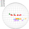 |
Fig. 1. Locations on the Sun of each of the IRIS burst profiles studied in this article, with different colours corresponding to different ARs. IRIS burst profiles are detected in multiple rasters sampled over multiple days for six of the seven ARs. Clearly, no IRIS burst profiles were detected at any time within AR 11871. General information about the identified IRIS burst profiles is presented in Table A.1. |
Given longer exposure times may lead to an increase in the number of saturated pixels (which are removed from the sample before the algorithm is applied), it is also important to investigate the numbers of potential IRIS burst profiles removed from each of these datasets before any additional analysis is conducted. In order to test this, we identified all pixels which were saturated (counts > 16 180) at one or more spectral positions in the wavelength range 1393.75 ± 0.2 Å. In total 239 pixels matched this criterion across all 42 datasets with approximately 100 of these appearing to be caused by cosmic ray spikes and another 100 appearing to be some other kind of burst, with relatively narrow spectra and no absorption lines over-laid on the Si IV 1394 Å spectra. This, therefore, left around 40 potential IRIS burst profiles which were spread across four datasets. Around half of these saturated potential IRIS burst profiles were found in the first dataset sampling AR 11916, which already contained 715 IRIS burst profiles, whilst the others were detected in the seventh raster to sample AR 11916, the first raster sampling AR 12104, and the third raster sampling AR 12104. Overall, the small numbers of saturated pixels displaying potential IRIS burst profiles (less than 1% of the sample studied here) and the centralisation of these to only a small number of datasets indicates that the removal of saturated pixels does not overly influence the results obtained in this manuscript.
We also made use of data from SDO’s Helioseismic and Magnetic Imager (SDO/HMI; Scherrer et al. 2012) in order to study the line-of-sight (LOS) magnetic field co-spatial to the IRIS observations. Full-disk LOS magnetic field maps were downloaded with a cadence of one hour in the time-period spanning from six hours prior to the start time of the first IRIS raster to six hours after the end time of the last IRIS raster for each AR. A zoomed 180″ × 180″ field-of-view (FOV) cut-out was then created co-temporal to the first IRIS scan centred on the pointing co-ordinates of that raster. All other SDO/HMI frames were then de-rotated to that time, before a co-spatial cut-out was constructed in order to create a consistent FOV through the entire time-period. Comparisons of these SDO/HMI maps with plage regions in the IRIS rasters indicated that these alignments were reasonable (estimated errors < 5″). As we only study the overall behaviour of the magnetic field within the entire ARs and the general structure of the magnetic field co-spatial to the IRIS burst profiles through time, no further alignment between instruments was conducted. These SDO/HMI data have a post-reduction pixel scale of 0.6″ which is more than adequate for investigating the overall behaviour of these ARs.
2.2. Modifications to the IRIS burst detection algorithm
To detect IRIS burst profiles, the algorithm of Kleint & Panos (2022) was used with slight modifications applied in order to both be able to study rasters that may have a small number of IRIS burst profiles and fix two minor bugs, which became apparent during this analysis. To tackle the first issue, the criterion of requiring at least 30 potential IRIS burst profiles applied by Kleint & Panos (2022) was dropped and any observation that had at least one candidate IRIS burst profile was analysed further. This increased the sample of IRIS burst profiles detected within these 42 rasters from 2462 to 3113 (a 26.44% increase). Following this adaption, the first bug, related to times when the IRIS orbit passes through the South Atlantic Anomaly (SAA) and hence returns noisy spectra, became apparent in the results. Specifically, the IRIS FITS SAA level2 keyword defaults to the value that is true for most of the observation. Therefore, observations where more time was spent in the SAA than outside of the SAA (which is very rare) will have this keyword set to 1 at all times and were, thus, excluded in the first version of the pipeline. The first version of the pipeline correctly queried the level1 data, which includes the actual flag for SAA/no SAA and updated the corresponding header entry in the level2 data to 1 during times of SAA. However, it did not check if the header entry may already be set to 1 due to the convention of the level2 data for SAA dominant datasets, even though no SAA occurred at the specific time when the spectra were sampled. The new version of the pipeline does both checks.
The second bug is related to the fact that the Si IV observing window width changed slightly with the evolution of the IRIS linelists, and between the different types of linelists. The original pipeline had a bug with extrapolations of spectra, leading to unintended values far away from the Si IV lines. This did not affect strong bursts (since the signal is near the line center and the continuum is close to zero due to the normalization), which have always been classified properly, but it could mistakenly classify noisy burst spectra into a non-burst category. Extrapolated values are now properly set to zero and thus do not affect the classification. The classification in Kleint & Panos (2022) focused on minimizing false-positives and if in doubt, a spectrum was excluded from being of burst-type so this should not have influenced their results excessively. Applying the algorithm following these subsequent modifications increased the sample further from 3113 IRIS burst profiles to a total of 4019 IRIS burst profiles (a further increase of 29.10%). These new IRIS burst profiles mostly have very weak absorption lines and/or are noisy, but do visually look like bursts so are included here for completeness. Notably, these events were detected across a total of 35 datasets, up from 15 using the algorithm before removal of the 30 spectra criterion and the subsequent modifications.
It should be mentioned, however, that the variety of burst spectra makes it impossible to catch every single burst with a classification template of “only” 423 different spectral types. We are confident, though, that the most common types of burst spectra are identified reliably. An example of an IRIS burst profile which was not detected by the pipeline is displayed in Fig. 2. In the left-hand panel we plot the intensity of the Si IV 1394 Å line core for the fourth raster sampling AR 12104 (i.e. the raster where IRIS bursts were detected manually but not automatically). The locations where IRIS passed through the SAA during this observation are marked by the red arrows. The orange circles outline two pixels, one containing a manually detected IRIS burst profile and one containing a non-burst profile, chosen for reference. In the right-hand panels, the black lines plot the observed spectra at each of these pixels with clear, albeit shallow, absorption blends indicative of an IRIS burst profile visible on the top panel. The blue lines plot the reference spectra deemed to be the closest mathematically to the observed spectra which in both cases is a non-burst reference spectra. The orange line included on the top panel plots the closest IRIS burst reference spectrum to this spectrum, which was mathematically ‘further’ from the observed spectrum than the non-burst reference spectrum (distance of 0.83 compared to a distance of 0.52). The only way to improve detections of such bursts would be to increase the number of template reference spectra from the 423 currently used. Given we only found a very small number (around ten) of additional IRIS burst profiles through our manual checks, and adding further reference spectra risks increasing the rate of false detections, we did not deem this necessary for this study.
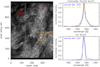 |
Fig. 2. Example of IRIS burst profiles missed by the algorithm. Left-hand panel: intensity of the FOV during the fourth IRIS raster sampling AR 12104 at the core wavelength of the Si IV 1394 line (logarithmically scaled to enhance contrast). Our algorithm did not identify any bursts in this raster. The two times during which IRIS passed through the SAA, thereby causing noisy spectra, during this observation are marked by red arrows. The orange circles locate two pixels whose spectra are shown in the right-hand panels (black lines), one containing a manually detected burst and the other containing no burst spectra. Right-hand panels: two IRIS spectra selected to demonstrate how a small number of IRIS burst profiles may be missed by the algorithm. The top panel plots a manually detected IRIS burst with a clear, albeit shallow, absorption blend over-laid on the Si IV 1394 Å line, while the bottom panel is a typical non-burst spectrum. Both spectra are normalised to their peak intensity. We over-plot the mathematically closest reference spectrum considered by the algorithm to each of these profiles (blue lines), which in both cases is a non-burst reference spectrum. Therefore, no IRIS burst profile is found for either pixel by the algorithm. The nearest IRIS burst reference spectrum to the manually detected IRIS burst profile is also over-plotted on the top panel for reference (orange line). |
3. Results and discussion
3.1. General AR properties
To begin our analysis, we investigated the general properties of each AR in order to better contextualise any subsequent inferences about IRIS bursts. Firstly, we identified the number of raster scans which displayed IRIS burst profiles for each AR finding varying behaviour. Of the seven ARs studied here, five (11850, 11909, 11916, 12104, and 12139) contained IRIS burst profiles in each raster scan, including both IRIS burst profiles detected using automated methods and those identified through the subsequent manual analysis. AR 11916 contained the most automatically detected IRIS burst profiles, with 2052 (51.06% of the total sample studied here) being identified over the eight rasters analysed, whilst the other four ARs each contained between 1144 and 168 automatically detected IRIS burst profiles. On top of this, one AR (11856) was found to contain IRIS burst profiles in some but not all rasters and one AR (11871) was found to contain no IRIS burst profiles at any time. This analysis indicates that the age of the AR is not a defining factor in whether IRIS burst profiles are present with the two youngest ARs (11871 and 11916), which both emerged onto the solar disk in the three days prior to the IRIS scans, displaying sharply contrasting behaviour.
Secondly, we calculated the total unsigned magnetic flux within a zoomed 180″ × 180″ FOV around each AR at each SDO/HMI time-step. Interestingly, the five ARs which contained IRIS burst profiles in each raster had the five highest peak fluxes (1.44 × 10²¹ Mx, 1.66 × 10²¹ Mx, 1.91 × 10²¹ Mx, 2.23 × 10²¹ Mx, and 1.50 × 10²¹ Mx for ARs 11850, 11909, 11916, 12104, and 12139, respectively) with each exceeding 1021 Mx. The remaining two ARs, which contained either a small number or zero IRIS burst profiles, both had peak fluxes of less than 1021 Mx (8.60 × 1020 Mx and 5.38 × 10²⁰ Mx for ARs 11856 and 11871, respectively). In the left-hand column of Fig. 3, we plot 100″ × 100″ zoomed SDO/HMI images sampled at the time at which the peak unsigned magnetic flux was measured for three ARs (11850, 11871, and 11916 from top to bottom, respectively). The middle column of Fig. 3 plots the IRIS Si IV 1394 Å line core intensity across this FOV sampled at the closest raster to the SDO/HMI images, with the pointing corrected for solar rotation. The red contours over-laid on the SDO/HMI images outline the locations of the IRIS burst profiles identified in these rasters using automated methods. The right-hand column of Fig. 3 plots the evolution of the total unsigned magnetic flux (solid line), positive flux (dashed line), and negative flux (dotted line) calculated from the larger 180″ × 180″ SDO/HMI FOV with time. Clearly, ARs 11916 and 11850 are more complex in their magnetic structuring (left-panels of Fig. 3) and have total unsigned magnetic fluxes which initially increase before reaching a peak and then decreasing (right-panels of Fig. 3). On the other hand, AR 11871 is less complex and has a total unsigned magnetic flux which slowly decreases with time. Our results indicate that the total unsigned magnetic flux and the complexity of the structuring of that flux within an AR may be a dominant factor determining whether IRIS bursts are widely detected or not, rather than the age of the AR.
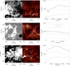 |
Fig. 3. Context plots for three of the ARs, namely ARs 11850, 11871, and 11916 from top to bottom, studied. Left-hand column: zoomed 100″ × 100″ SDO/HMI magnetic context images. The plotted frames were selected as they contained the peak total unsigned magnetic flux for these regions during the time studied. Middle column: Si IV 1394 Å line core intensity sampled from the IRIS raster with start time closest to the SDO/HMI images plotted in the left hand column. The pointing of the IRIS FOV was de-rotated to the SDO/HMI observation time. Right-hand column: evolution of the total unsigned (solid lines), positive (dashed lines), and negative (dotted lines) magnetic flux within the wider 180″ × 180″ FOV through the time-period studied here for each AR. The red contours over-laid on the left-hand column outline the IRIS burst profiles returned using automated methods from the IRIS raster plotted in the respective middle column. The five ARs with the highest peak magnitudes of the unsigned flux were found to contain the majority of the IRIS burst profiles identified here. |
3.2. Spatial properties of IRIS burst profiles
We continued our analysis by grouping the 4019 IRIS burst profiles identified here into separate, connected objects which we define as parent IRIS bursts. To achieve this, we created binary maps of the locations of IRIS burst profiles within each raster scan and then combined IRIS burst profiles which were adjacent in the x − y plane together into parent IRIS bursts. If two parent IRIS bursts were separated by even one pixel, we considered that they were different events. Additionally, if the observational routine had more than one raster then only the middle raster was considered here in order to avoid longer-lived parent IRIS bursts, potentially present in repeated rasters, being counted multiple times. Importantly, our analysis of these parent UV bursts does not include any temporal component. This stipulation only removed 119 IRIS burst profiles from our sample meaning it should not have a major influence on our results. Overall, this analysis returned 752 parent IRIS bursts spread across the 35 IRIS rasters. In the left-hand panel of Fig. 4, we plot an example of a binary map displaying the locations of numerous IRIS burst profiles from one specific raster within AR 11850. This plot is calculated from the dataset which was used by Peter et al. (2014) to originally identify IRIS bursts, with the four largest parent IRIS bursts corresponding to the four events studied by those authors. This clearly shows the effectiveness of the algorithm developed by Kleint & Panos (2022) and modified here. The zoomed cut-out over-laid on this panel more clearly displays how adjacent IRIS burst profiles are combined to form separate parent IRIS bursts. Nine parent IRIS bursts are present within this small FOV, with each event being plotted in a different colour.
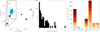 |
Fig. 4. Structuring of IRIS burst profiles in these datasets. Left-hand panel: binary map showing the locations of IRIS burst profiles (black pixels) identified within a single raster sampling AR 11850. Four of the parent IRIS bursts within this raster correspond to the four events studied in Peter et al. (2014). The over-lying cut-out displays how connected objects are combined to form parent IRIS bursts, with nine events (all individually coloured) occurring in this small region. Middle panel: histogram of parent IRIS burst area against frequency constructed using all 42 datasets, where the y-axis is plotted in logarithmic scale. Each bar is binned over a range of 0.3 arcsec2 (corresponding to five pixels). Right-hand panel: bar chart plotting the number of parent IRIS bursts by AR. The different coloured sections of each bar indicate the number of parent IRIS bursts identified in different rasters sampling that AR, with the light yellow at the bottom corresponding to the first raster within which IRIS bursts were detected using automated methods for that specific AR. The progressively darker colours up the bars correspond to the subsequent rasters within which IRIS bursts were detected. The physical number of bursts plotted in each bar segment can be found in Table A.1. |
In the middle panel of Fig. 4, we plot a histogram of parent IRIS burst area against frequency for all of the 752 identified events. The histogram is binned across 0.3 arcsec2 (five pixels) and the y-axis is plotted using a logarithmic scale. Clearly, the majority of the studied events are small, with 383 of these parent IRIS bursts having areas of only one pixel. The mean area of this sample of parent IRIS bursts is 0.31 arcsec2 (corresponding to 5.19 pixels); however, the distribution is non-Gaussian and the standard deviation of this sample is 0.72 arcsec2 (12.18 pixels), more than double the mean, suggesting one should not interpret this as a precise estimate. Our results do, though, clearly indicate that the majority of parent IRIS bursts are extremely small-scale. Notably, several larger brightenings in the Si IV 1394 Å line core are found to contain numerous parent IRIS bursts through our analysis. For example, one 6.30″ × 2.72″ region in the second raster sampling AR 12104 (around xc ≈ 200″, yc ≈ −296″) was found to contain 20 parent IRIS bursts, with an average area of 0.12 arcsec2 (corresponding to 1.57 pixels). From the entire sample studied here, only 52 parent IRIS bursts (6.91%) have an area over 1 arcsec2 (corresponding to 17 pixels) with 28 of these occurring in AR 11916. The largest parent IRIS burst occurred in AR 11916 and had an area of 8.98 arcsec2 (corresponding to 151 pixels), much larger than the typical sizes of UV bursts in general (see Young et al. 2018).
In the right-hand panel of Fig. 4, we plot a bar chart displaying the number of parent IRIS bursts identified per AR. The colours in each bar indicate parent IRIS bursts identified in different rasters, with the bottom (light yellow) portion corresponding to the first raster within which IRIS burst profiles were identified for that specific AR. A high proportion of the parent IRIS bursts were found within ARs 11850 and 11916 (70.61% of the total sample) whilst AR 11871 contains zero parent IRIS bursts. The highest number of parent IRIS bursts in a single raster was 65, which were identified in the first raster sampling AR 11916, with the mean number of parent IRIS bursts per raster being 17.90. The average area of the parent IRIS bursts was found to change in a seemingly random way from raster to raster (neither monotonically increasing or decreasing) as the host ARs evolved. In total, ten rasters within the sample analysed here contained more than 30 parent IRIS bursts, with five of these occurring in AR 11916, three occurring in AR 11850, and one occurring in both ARs 12104 and 12139. Overall, these results imply a parent IRIS burst spatial frequency of 0.00069 arcsec−2 in ARs, well below the spatial frequency of, for example, spicules in the chromosphere. See Table A.1 for a summary of these findings.
3.3. Locations of IRIS burst profiles within ARs
One of the main aims of this research is to identify whether IRIS burst profiles are detected randomly across ARs or whether they are confined to consistent localised regions through time. In order to analyse this, we studied the locations of IRIS burst profiles within the two ARs (namely ARs 11850 and 11916) for which more than 100 IRIS burst profiles were detected using the algorithm in more than one raster. We de-rotated each raster to a consistent pointing which we refer to as the origin (0″, 0″), constructed binary maps of the locations of IRIS burst profiles, and then calculated the centres-of-mass of IRIS burst profiles for each raster. In Fig. 5, we plot a visualisation of this analysis on maps of the Si IV 1394 Å line core intensity (logarithmically scaled) from one representative raster for each AR (11850 in the left-hand panel and 11916 in the right-hand panel). The over-laid contours denote the locations of IRIS burst profiles and the crosses indicate the centres-of-mass for each specific raster. The relationship between colour and raster number is consistent with the colours used in the right-hand panel of Fig. 4.
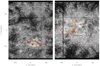 |
Fig. 5. Spatial positions of IRIS burst profiles through time in two datasets. Left-hand panel: map of the Si IV 1394 Å line core intensity (logarithmically scaled) within AR 11850 sampled during the raster starting at 05:59:43 UT on 26th September 2013. Right-hand panel: same as the left-hand panel but for AR 11916 sampled during the raster starting at 03:09:49 UT on 7th December 2013. The contours and crosses over-laid on both panels denote the IRIS burst profiles and their centres-of-mass, respectively, for each raster containing more than 100 automatically detected IRIS burst profiles. The colours indicate different rasters and are consistent with those used in the right-hand panel of Fig. 4. |
For both ARs, IRIS burst profiles were found to be predominantly localised to relatively small regions, with approximate areas of 100″ × 60″. The centres-of-mass of IRIS burst profiles also appeared to be consistent through time for both ARs, only varying by a maximum of 31.11″ in AR 11850 and 37.96″ in AR 11916. In general, the locations of IRIS burst profiles within the ARs appeared to be limited to the most pronounced polarity inversion lines, as would be expected for events hypothesised to be driven by magnetic reconnection. Interestingly, IRIS burst profiles in both of these ARs appeared to become more spatially separated through time, with the contours in Fig. 5 appearing further away from the centres-of-mass for subsequent rasters. In order to investigate this, we calculated the average separation between the IRIS burst profiles and the centres-of-mass through time for the rasters containing more than 100 IRIS burst profiles. For AR 11850, this separation increased from 13.00″ (±10.42″) to 45.46″ (±9.20″) over the five rasters studied here; whilst for AR 11916, the average separation increased from 9.51″ (±10.32″) to 32.10″ (±15.07″) over the first five rasters before decreasing again to 18.63″ (±15.04″) by the sixth raster. Although this analysis indicates there may be an increase in the separation of IRIS burst profiles within an AR as it evolves, we note that two ARs were studied and large standard deviations were calculated, meaning this result is still tentative and requires further analysis using a larger sample of ARs in the future.
3.4. Spectral properties of IRIS burst profiles
To continue our analysis, we next investigated whether several spectral properties of IRIS burst profiles varied systematically during the evolution of ARs or whether they remained relatively consistent. Once again, only rasters within ARs 11850 (left-hand panels) and 11916 (right-hand panels) which contained more than 100 IRIS burst profiles were studied in order to provide appropriate statistics. In Fig. 6, we plot the distributions of three parameters calculated from the Si IV 1394 Å spectra sampled at all pixels automatically identified as IRIS burst profiles, for the appropriate rasters. The top panels plot the mean intensity (logarithmically scaled) from a ±0.075 Å window around the Si IV 1394 Å line core, the middle panels plot the logarithmically scaled peak intensity of the Si IV 1394 Å line for the identified IRIS burst profiles, whilst the bottom panels plot the spectral positions where the maximum intensity was measured for each IRIS burst profile. The diamonds on each distribution indicate the mean value calculated for that raster, and the top and bottom crosses plot the 75th and 25th percentile values, respectively. Overall, although some changes in the distributions are observed between specific rasters, no systematic changes (e.g. monotonic intensity increases, transitions from blue to red shifts) in these parameters is detected as the ARs age.
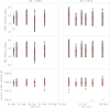 |
Fig. 6. Distributions of various spectral parameters for all IRIS burst profiles identified within datasets sampling ARs 11850 (left-hand panels) and 11916 (right-hand panels). Only datasets which returned more than 100 IRIS burst profiles were considered. Top panels: logarithmic mean intensity from a ±0.075 Å window surrounding the Si IV 1394 Å line core calculated for each IRIS burst profile. Middle panels: logarithmic maximum intensity for each IRIS burst profile. Bottom panels: spectral location of the maximum intensity of each IRIS burst profile. The diamonds indicate the mean for each raster, while the upper and lower crosses indicate the 75th and 25th percentiles, respectively. No systematic or monotonic changes in these parameters through time are apparent. |
Following on from this, we also studied which reference spectra were returned the most frequently as the ‘closest’ fits to the IRIS burst profiles identified in each of these rasters. This analysis allowed us to infer whether any changes in the common spectral shapes of IRIS burst profiles are present through time. In these datasets, no single reference spectrum was found to be the most accurate mathematical match to more than 7.34% of all of the IRIS burst profiles within a single raster. Additionally, unique reference spectra were found to make up, on average across these datasets, 47.57% of all of the observed spectra indicating that a huge variety of spectral shapes of IRIS burst profiles exist for each dataset. These two combined facts suggest that no preferential reference spectrum is present in any given raster, with the identified IRIS burst profiles being randomly spread between different reference spectra.
3.5. Relations to the local LOS magnetic field
Our final analysis focused on the relationship between the parent IRIS bursts identified in this study and the co-spatial under-lying LOS magnetic field structure as inferred by the SDO/HMI instrument. It is well known that IRIS bursts often occur co-spatial to regions of opposite polarity magnetic field (see, for example, Young et al. 2018) where magnetic reconnection is thought to be possible in the lower solar atmosphere. As the SDO/HMI instrument has a spatial resolution of approximately 1″, we only studied parent IRIS bursts with areas greater than 1 arcsec2 (corresponding to approximately 17 pixels). Additionally, we removed the parent IRIS bursts with areas above 4 arcsec2 (corresponding to 70 pixels) as the foot-points of those events would be difficult to define in a consistent manner. These stipulations left 46 parent IRIS bursts for analysis. In Fig. 7, we plot the LOS magnetic field saturated at ±100 G sampled for a 5″ × 5″ FOV surrounding the centre of each parent IRIS burst. The red and blue contours outline positive and negative polarity LOS magnetic fields at values of 20 G and −20 G, respectively, while the orange contours outline the locations of the parent IRIS bursts. The magnetic field map for each event was constructed by de-rotating the closest temporal frame in the respective one hour cadence SDO/HMI dataset to the time at which the parent IRIS burst was detected, meaning the locations of the bursts with respect to the magnetic field are only an approximation. Although this method will have some inherent errors on small-scales, the alignment appears to work well for the full FOV (as can be seen in Fig. 3) giving us confidence that a closer alignment is not required for this general analysis.
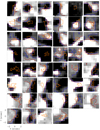 |
Fig. 7. LOS magnetic field maps co-spatial to the 46 parent IRIS bursts with measured areas between 1 arcsec2 and 4 arcsec2. Each plot covers a region of 5″ × 5″ centred on the location of the parent IRIS burst from the closest SDO/HMI image in time, de-rotated to the time of IRIS burst profile detection. The red and blue contours outline regions of positive and negative magnetic fields saturated at 20 G and −20 G, respectively, whilst the orange contours outline the approximate locations of the parent IRIS bursts. Opposite polarity magnetic fields are found within the FOV for 43 (93%) of these parent IRIS bursts. |
Overall, 43 (93%) of the panels plotted in Fig. 7 contain bi-poles in the LOS magnetic field within the 5″ × 5″ surrounding the parent IRIS bursts. For the three remaining events, one occurs co-spatial to an apparently uni-polar region of positive polarity flux and the other two occur co-spatial to apparently uni-polar regions of negative polarity flux. As the magnetic field maps could have been measured up to ±30 min around the detection of the parent IRIS burst, we note that these magnetic field maps may not be entirely representative of the exact magnetic field structure at the time of potential reconnection as, for example, cancellation could have occurred removing evidence of any bi-poles (see for example, Nelson et al. 2016) for the three uni-polar events. Additionally, the spatial resolution of the SDO/HMI instrument may be insufficient for resolving all of the magnetic field elements at these locations (as discussed by Reid et al. 2016) which could cause us to detect a uni-polar region when a bi-polar region was actually present. It is clear, however, that the majority of parent IRIS bursts with areas between 1 arcsec2 and 4 arcsec2 occur co-spatial to regions of opposite polarity magnetic field in the lower solar atmosphere, supporting the assertion that these events could be driven by magnetic reconnection.
4. Conclusions
In this article, we used a slightly modified (see Sect. 2.2) version of the algorithm originally applied in Kleint & Panos (2022) in order to investigate whether changes in the measurable properties of IRIS burst profiles occurred as their host ARs evolved. We studied 42 dense IRIS rasters which each sampled one of seven host ARs, with each AR being sampled at least four times. We found:
-
The maximum total unsigned magnetic flux within an AR, and the complexity of the structuring of that flux, may be important as an indicator of whether IRIS burst profiles are present. The two ARs with the lowest peak total unsigned magnetic fluxes contained far fewer IRIS burst profiles than the five ARs with the highest unsigned magnetic fluxes. Specifically, AR 11871 (with a peak unsigned magnetic flux of 5.38 × 10²⁰) was found to contain no IRIS burst profiles in the four rasters which sampled it, whilst AR 11856 (with a peak unsigned magnetic flux of 8.60 × 10²⁰ was found to contain only 25 IRIS burst profiles (0.62% of the total number of IRIS burst profiles studied here) across the five rasters which sampled it. The age of the AR was not found to influence the number of IRIS burst profiles returned by the algorithm, with the two youngest ARs (11916 and 11871) being found to contain the most and least IRIS burst profiles, respectively.
-
In total, 4019 IRIS burst profiles were returned by the algorithm from these 42 rasters, with these being found to belong to 752 parent IRIS bursts. These parent IRIS bursts had a mean area of 0.31 arcsec2, with 93.09% of the identified events having areas below 1 arcsec2 (centre panel of Fig. 4). We note that the mean area should not be over-interpreted due to the large standard deviation from this dataset (0.72 arcsec2) but it can be used to show that these events are typically small-scale. The frequencies and areas of these features did not monotonically increase or decrease as the host ARs evolved but instead varied in a seemingly randomly manner from raster to raster. The largest parent IRIS burst found through this analysis had an apparent area of 8.98 arcsec2 (corresponding to 151 pixels). The overall spatial frequency of IRIS burst profiles across the studied ARs was calculated to be 0.00069 arcsec−2, well below the coverage of spicules, for example.
-
IRIS burst profiles are typically confined to localised regions (around 100″ × 60″ for the two ARs studied here) close to the cores of ARs (as is displayed in Fig. 5). The average spatial separation between the centre-of-mass of all IRIS burst profiles within a raster and the individual IRIS burst profiles themselves appeared to increase with time in ARs 11850 and 11916 (the only ARs which contained more than 100 IRIS burst profiles in multiple rasters), suggesting IRIS bursts occurred across a larger area as their host ARs evolved. This increase in area potentially corresponds to the growth of the ARs themselves. These results suggest that one must be very careful when selecting appropriate targets for co-observations of IRIS burst-Ellerman bomb pairs with ground-based telescopes with limited FOVs, e.g. with the Daniel K. Inouye Solar Telescope (DKIST; Rimmele et al. 2020; Rast et al. 2021).
-
The spectral properties (e.g. peak intensities, spectral locations of the peak intensities) of IRIS burst profiles varied in a non-monotonic way in datasets sampling ARs 11850 and 11916 which contained more than 100 IRIS burst profiles, and then only slightly, through time. On top of this, the automatically detected IRIS burst profiles were found to be spread across a large number of the reference spectra used by the detection algorithm with, on average, unique reference spectra equalling 47.57% of the total number of IRIS burst profiles in any given raster. Additionally, no individual reference spectrum was found to be the best fit for more than 7.34% of the IRIS burst profiles returned for any given raster. These combined result indicate that no ‘typical’ IRIS burst spectra exists for the rasters studied here.
-
93% of all parent IRIS bursts with areas between 1 arcsec2 and 4 arcsec2 occurred co-spatial to bi-poles in the solar photosphere. This result further supports the assertion that these events are driven by magnetic reconnection in the lower solar atmosphere (Peter et al. 2014; Vissers et al. 2015; Hansteen et al. 2017).
Expanding this research to include a larger number of ARs (i.e. those sampled after 2014) will allow us to make further inferences about IRIS bursts in the future.
Acknowledgments
C.J.N. is thankful to ESA for support as an ESA Research Fellow. L.K. gratefully acknowledges funding via a SNSF PRIMA grant. IRIS is a NASA small explorer mission developed and operated by LMSAL with mission operations executed at NASA Ames Research Center and major contributions to downlink communications funded by ESA and the Norwegian Space Centre. SDO/HMI data provided courtesy of NASA/SDO and the HMI science team. This research has made use of NASA’s Astrophysics Data System Bibliographic Services.
References
- Berghmans, D., Auchère, F., Long, D. M., et al. 2021, A&A, 656, L4 [NASA ADS] [CrossRef] [EDP Sciences] [Google Scholar]
- Chen, Y., Przybylski, D., Peter, H., et al. 2021, A&A, 656, L7 [NASA ADS] [CrossRef] [EDP Sciences] [Google Scholar]
- Danilovic, S. 2017, A&A, 601, A122 [NASA ADS] [CrossRef] [EDP Sciences] [Google Scholar]
- De Pontieu, B., Title, A. M., Lemen, J. R., et al. 2014, Sol. Phys., 289, 2733 [Google Scholar]
- Dere, K. P., Bartoe, J. D. F., & Brueckner, G. E. 1989, Sol. Phys., 123, 41 [Google Scholar]
- Ellerman, F. 1917, ApJ, 46, 298 [NASA ADS] [CrossRef] [Google Scholar]
- Fang, C., Tang, Y. H., Xu, Z., Ding, M. D., & Chen, P. F. 2006, ApJ, 643, 1325 [Google Scholar]
- Hansteen, V. H., Archontis, V., Pereira, T. M. D., et al. 2017, ApJ, 839, 22 [NASA ADS] [CrossRef] [Google Scholar]
- Harrison, R. A. 1997, Sol. Phys., 175, 467 [Google Scholar]
- Hong, J., Ding, M. D., Li, Y., Fang, C., & Cao, W. 2014, ApJ, 792, 13 [NASA ADS] [CrossRef] [Google Scholar]
- Hong, J., Carlsson, M., & Ding, M. D. 2017, ApJ, 845, 144 [NASA ADS] [CrossRef] [Google Scholar]
- Judge, P. G. 2015, ApJ, 808, 116 [NASA ADS] [CrossRef] [Google Scholar]
- Kleint, L., & Panos, B. 2022, A&A, 657, A132 [NASA ADS] [CrossRef] [EDP Sciences] [Google Scholar]
- Lemen, J. R., Title, A. M., Akin, D. J., et al. 2012, Sol. Phys., 275, 17 [Google Scholar]
- Mandal, S., Peter, H., Chitta, L. P., et al. 2021, A&A, 656, L16 [NASA ADS] [CrossRef] [EDP Sciences] [Google Scholar]
- Nelson, C. J., Scullion, E. M., Doyle, J. G., Freij, N., & Erdélyi, R. 2015, ApJ, 798, 19 [Google Scholar]
- Nelson, C. J., Doyle, J. G., & Erdélyi, R. 2016, MNRAS, 463, 2190 [NASA ADS] [CrossRef] [Google Scholar]
- Nelson, C. J., Freij, N., Reid, A., et al. 2017, ApJ, 845, 16 [Google Scholar]
- Panesar, N. K., Tiwari, S. K., Berghmans, D., et al. 2021, ApJ, 921, L20 [CrossRef] [Google Scholar]
- Panos, B., & Kleint, L. 2021, ApJ, 915, 77 [NASA ADS] [CrossRef] [Google Scholar]
- Panos, B., Kleint, L., & Voloshynovskiy, S. 2021, ApJ, 912, 121 [NASA ADS] [CrossRef] [Google Scholar]
- Peter, H., Tian, H., Curdt, W., et al. 2014, Science, 346, 1255726 [Google Scholar]
- Rast, M. P., Bello González, N., Bellot Rubio, L., et al. 2021, Sol. Phys., 296, 70 [NASA ADS] [CrossRef] [Google Scholar]
- Reid, A., Mathioudakis, M., Doyle, J. G., et al. 2016, ApJ, 823, 110 [Google Scholar]
- Reid, A., Mathioudakis, M., Kowalski, A., Doyle, J. G., & Allred, J. C. 2017, ApJ, 835, L37 [NASA ADS] [CrossRef] [Google Scholar]
- Rimmele, T. R., Warner, M., Keil, S. L., et al. 2020, Sol. Phys., 295, 172 [Google Scholar]
- Scherrer, P. H., Schou, J., Bush, R. I., et al. 2012, Sol. Phys., 275, 207 [Google Scholar]
- Tian, H., Xu, Z., He, J., & Madsen, C. 2016, ApJ, 824, 96 [CrossRef] [Google Scholar]
- Vissers, G., & Rouppe van der Voort, L. 2012, ApJ, 750, 22 [Google Scholar]
- Vissers, G. J. M., Rouppe van der Voort, L. H. M., & Rutten, R. J. 2013, ApJ, 774, 32 [NASA ADS] [CrossRef] [Google Scholar]
- Vissers, G. J. M., Rouppe van der Voort, L. H. M., Rutten, R. J., Carlsson, M., & De Pontieu, B. 2015, ApJ, 812, 11 [NASA ADS] [CrossRef] [Google Scholar]
- Young, P. R., Tian, H., Peter, H., et al. 2018, Space Sci. Rev., 214, 120 [Google Scholar]
Appendix A: Summary of observations and results
Summary of the 42 datasets studied in this article.
All Tables
All Figures
|
Fig. 1. Locations on the Sun of each of the IRIS burst profiles studied in this article, with different colours corresponding to different ARs. IRIS burst profiles are detected in multiple rasters sampled over multiple days for six of the seven ARs. Clearly, no IRIS burst profiles were detected at any time within AR 11871. General information about the identified IRIS burst profiles is presented in Table A.1. |
| In the text | |
|
Fig. 2. Example of IRIS burst profiles missed by the algorithm. Left-hand panel: intensity of the FOV during the fourth IRIS raster sampling AR 12104 at the core wavelength of the Si IV 1394 line (logarithmically scaled to enhance contrast). Our algorithm did not identify any bursts in this raster. The two times during which IRIS passed through the SAA, thereby causing noisy spectra, during this observation are marked by red arrows. The orange circles locate two pixels whose spectra are shown in the right-hand panels (black lines), one containing a manually detected burst and the other containing no burst spectra. Right-hand panels: two IRIS spectra selected to demonstrate how a small number of IRIS burst profiles may be missed by the algorithm. The top panel plots a manually detected IRIS burst with a clear, albeit shallow, absorption blend over-laid on the Si IV 1394 Å line, while the bottom panel is a typical non-burst spectrum. Both spectra are normalised to their peak intensity. We over-plot the mathematically closest reference spectrum considered by the algorithm to each of these profiles (blue lines), which in both cases is a non-burst reference spectrum. Therefore, no IRIS burst profile is found for either pixel by the algorithm. The nearest IRIS burst reference spectrum to the manually detected IRIS burst profile is also over-plotted on the top panel for reference (orange line). |
| In the text | |
|
Fig. 3. Context plots for three of the ARs, namely ARs 11850, 11871, and 11916 from top to bottom, studied. Left-hand column: zoomed 100″ × 100″ SDO/HMI magnetic context images. The plotted frames were selected as they contained the peak total unsigned magnetic flux for these regions during the time studied. Middle column: Si IV 1394 Å line core intensity sampled from the IRIS raster with start time closest to the SDO/HMI images plotted in the left hand column. The pointing of the IRIS FOV was de-rotated to the SDO/HMI observation time. Right-hand column: evolution of the total unsigned (solid lines), positive (dashed lines), and negative (dotted lines) magnetic flux within the wider 180″ × 180″ FOV through the time-period studied here for each AR. The red contours over-laid on the left-hand column outline the IRIS burst profiles returned using automated methods from the IRIS raster plotted in the respective middle column. The five ARs with the highest peak magnitudes of the unsigned flux were found to contain the majority of the IRIS burst profiles identified here. |
| In the text | |
|
Fig. 4. Structuring of IRIS burst profiles in these datasets. Left-hand panel: binary map showing the locations of IRIS burst profiles (black pixels) identified within a single raster sampling AR 11850. Four of the parent IRIS bursts within this raster correspond to the four events studied in Peter et al. (2014). The over-lying cut-out displays how connected objects are combined to form parent IRIS bursts, with nine events (all individually coloured) occurring in this small region. Middle panel: histogram of parent IRIS burst area against frequency constructed using all 42 datasets, where the y-axis is plotted in logarithmic scale. Each bar is binned over a range of 0.3 arcsec2 (corresponding to five pixels). Right-hand panel: bar chart plotting the number of parent IRIS bursts by AR. The different coloured sections of each bar indicate the number of parent IRIS bursts identified in different rasters sampling that AR, with the light yellow at the bottom corresponding to the first raster within which IRIS bursts were detected using automated methods for that specific AR. The progressively darker colours up the bars correspond to the subsequent rasters within which IRIS bursts were detected. The physical number of bursts plotted in each bar segment can be found in Table A.1. |
| In the text | |
|
Fig. 5. Spatial positions of IRIS burst profiles through time in two datasets. Left-hand panel: map of the Si IV 1394 Å line core intensity (logarithmically scaled) within AR 11850 sampled during the raster starting at 05:59:43 UT on 26th September 2013. Right-hand panel: same as the left-hand panel but for AR 11916 sampled during the raster starting at 03:09:49 UT on 7th December 2013. The contours and crosses over-laid on both panels denote the IRIS burst profiles and their centres-of-mass, respectively, for each raster containing more than 100 automatically detected IRIS burst profiles. The colours indicate different rasters and are consistent with those used in the right-hand panel of Fig. 4. |
| In the text | |
|
Fig. 6. Distributions of various spectral parameters for all IRIS burst profiles identified within datasets sampling ARs 11850 (left-hand panels) and 11916 (right-hand panels). Only datasets which returned more than 100 IRIS burst profiles were considered. Top panels: logarithmic mean intensity from a ±0.075 Å window surrounding the Si IV 1394 Å line core calculated for each IRIS burst profile. Middle panels: logarithmic maximum intensity for each IRIS burst profile. Bottom panels: spectral location of the maximum intensity of each IRIS burst profile. The diamonds indicate the mean for each raster, while the upper and lower crosses indicate the 75th and 25th percentiles, respectively. No systematic or monotonic changes in these parameters through time are apparent. |
| In the text | |
|
Fig. 7. LOS magnetic field maps co-spatial to the 46 parent IRIS bursts with measured areas between 1 arcsec2 and 4 arcsec2. Each plot covers a region of 5″ × 5″ centred on the location of the parent IRIS burst from the closest SDO/HMI image in time, de-rotated to the time of IRIS burst profile detection. The red and blue contours outline regions of positive and negative magnetic fields saturated at 20 G and −20 G, respectively, whilst the orange contours outline the approximate locations of the parent IRIS bursts. Opposite polarity magnetic fields are found within the FOV for 43 (93%) of these parent IRIS bursts. |
| In the text | |
Current usage metrics show cumulative count of Article Views (full-text article views including HTML views, PDF and ePub downloads, according to the available data) and Abstracts Views on Vision4Press platform.
Data correspond to usage on the plateform after 2015. The current usage metrics is available 48-96 hours after online publication and is updated daily on week days.
Initial download of the metrics may take a while.