| Issue |
A&A
Volume 666, October 2022
|
|
|---|---|---|
| Article Number | A99 | |
| Number of page(s) | 13 | |
| Section | Extragalactic astronomy | |
| DOI | https://doi.org/10.1051/0004-6361/202243390 | |
| Published online | 13 October 2022 | |
A study of globular clusters in a lenticular galaxy in Hydra I from deep HST/ACS photometry
1
Gran Sasso Science Institute, L’Aquila, Italy
e-mail: This email address is being protected from spambots. You need JavaScript enabled to view it.
2
INFN Laboratori Nazionali del Gran Sasso, L’Aquila, Italy
3
INAF – Osservatorio Astronomico d’Abruzzo, Teramo, Italy
4
University of Naples Federico II, Naples, Italy
5
INAF – Osservatorio Astronomico di Roma, Monte Porzio Catone, Roma, Italy
6
NSF’s NOIRLab, Tucson, AZ 85719, USA
Received:
21
February
2022
Accepted:
16
May
2022
Abstract
Aims. We take advantage of exquisitely deep optical imaging data from the Hubble Space Telescope’s Advanced Camera for Surveys (HST/ACS) in the F475W (gF475W) and F606W (VF606W) bands to study the properties of the globular cluster (GC) population in the intermediate-mass lenticular galaxy PGC 087327in the Hydra I galaxy cluster.
Methods. We inspected the photometric (magnitudes and colour) and morphometric (compactness, elongation, etc.) properties of sources lying in an area of ∼19 × 19 kpc centred on PGC 087327 and compared them with four neighbouring fields over the same HST/ACS mosaic. This allowed us to identify a list of GC candidates and to inspect their properties using a background decontamination method.
Results. Relative to four comparison fields, PGC 087327 shows a robust overdensity of GCs, NGC = 82 ± 9. At the estimated magnitude of the galaxy, this number implies a specific frequency of SN = 1.8 ± 0.7. In spite of the short wavelength interval available with the gF475W and VF606W passbands, the colour distribution shows a clear bimodality with a blue peak at ⟨gF475W − VF606W⟩ = 0.47 ± 0.05 mag and a red peak at ⟨gF475W − VF606W⟩ = 0.62 ± 0.03 mag. We also observe the typical steeper slope of the radial distribution of red GCs relative to blue ones. Thanks to the unique depth of the available data, we characterise the GC luminosity function (GCLF) well beyond the expected GCLF turnover. We find gTOMF475W = 26.54 ± 0.10 mag and VTOMF606W = 26.08 ± 0.09 mag, which after calibration yields a distance of DGCLF = 56.7 ± 4.3(statistical) ± 5.2(systematic) Mpc.
Key words: galaxies: distances and redshifts / galaxies: elliptical and lenticular, cD / galaxies: star clusters: general / galaxies: individual: PGC 087327
© N. Hazra et al. 2022
 Open Access article, published by EDP Sciences, under the terms of the Creative Commons Attribution License (https://creativecommons.org/licenses/by/4.0), which permits unrestricted use, distribution, and reproduction in any medium, provided the original work is properly cited.
This article is published in open access under the Subscribe-to-Open model. This email address is being protected from spambots. You need JavaScript enabled to view it. to support open access publication.
1. Introduction
Globular clusters (GCs) are dense stellar systems, with typically old ages, found ubiquitously in massive galaxies and spanning a wide range of magnitudes (e.g., Brodie & Strader 2006). The small number of available spectroscopic studies of extragalactic GCs inferred that the majority of them have ages comparable to galactic GCs (e.g., Cohen et al. 1998; Beasley & Sharples 2000; Kuntschner et al. 2002), namely t ≥ 10 Gyr (Carretta et al. 2000). In all cases where the population of GCs in a spheroidal galaxy, either elliptical or lenticular, was observed with an intermediate-age component (t ∼ 3 − 6 Gyr), this only composed a small fraction of the GC population, mostly in merger remnants such as NGC 3610 or NGC 1316 (Goudfrooij et al. 2001; Brodie & Strader 2006; Bassino & Caso 2017).
Throughout this paper we focus only on the old GCs component. They are often some of the most luminous non-transient objects in a galaxy and exhibit a variety of properties (magnitudes, colours, radial distributions, sizes, and so on) that are used as tracers of galaxy formation and evolution (e.g., Brodie & Strader 2006). These old GC systems have been used as distance indicators since Hanes (1977) due to the fact that they have a nearly universal Gaussian luminosity function with a peak at a constant absolute magnitude of  mag (Georgiev et al. 2009), known as the turnover magnitude. The near-universality of the globular cluster luminosity function (GCLF) in optical and near-IR bands has prompted its use as a standard candle to act as a secondary distance indicator (Ferrarese et al. 2000).
Old GC populations typically exhibit a bimodal colour distribution with a blue (metal-poor) and a red (metal-rich) peak. This has historically been attributed to hierarchical formation giving rise to two distinct GC sub-populations with different peak metallicities (Brodie & Strader 2006). Additionally, while the red GC system generally shows a radial profile that roughly matches the galaxy field star profile (Harris 2009), the blue, more metal-poor GCs are often observed to be less concentrated close to the galaxy core and more numerous than the red GCs at larger radii. This seems to be indicative of an in situ red GC population and of a blue population acquired through galaxy mergers and tidal events (Forbes et al. 2011).
However, recent works (Yoon et al. 2006; Richtler 2006; Cantiello et al. 2007; Cantiello & Blakeslee 2007, 2012, among others) have shown that the bimodality could also arise from a continuous metallicity distribution with a radial gradient combined with non-linear colour-metallicity relations. This could point to stochastic processes in galaxy formation, without requiring two major events or mechanisms to generate the two observed sub-populations.
In this work, we take advantage of the exquisite resolution of data from the Hubble Space Telescope’s Advanced Camera for Surveys (HST/ACS), combined with the extremely deep observations of NGC 3314A/B, to characterise the GC system in PGC 087327. In particular, we analyse the colour and radial distributions and the luminosity function of the old GCs in this galaxy.
PGC 087327 is an intermediate-mass galaxy (see Sect. 2) classified as E3/S0, close in projection to NGC 3314A/B, in the Hydra I cluster. Using the flow-corrected peculiar velocity from Cosmicflows-3 (Tully et al. 2016) reported in Table 1, and an H0 ∼ 73 km s−1 Mpc−1 (e.g., Blakeslee et al. 2021; Khetan et al. 2021), we obtain a preliminary estimate of the distance, D ∼ 61 Mpc. Later in this work, we use the photometry of GCs to derive a more refined estimate of this distance.
Main properties of PGC 087327.
This paper is organised as follows: we describe the observational dataset and target in Sect. 2 and the procedures to identify GC candidates in Sect. 3. The analysis of the main properties of the GC sample, along with the calibrations and results, are outlined in Sect. 4, and the conclusions are summarised in Sect. 5.
2. Observational data
2.1. Target properties
The main properties of PGC 087327 are given in Table 1. Figure 1 shows the colour composite image of the galaxy based on the HST data used in this work.
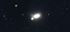 |
Fig. 1. Colour composite 2′ × 1′ HST image of PGC 087327. North is up and east is left. |
We derived an approximate estimate of the galaxy mass using stellar population models and empirical relations. For the estimate from models, we adopted the colour-mass-luminosity relations of Into & Portinari (2013, see their Table 3) together with the Ks magnitude (the magnitude from fit extrapolation; see Table 1) from the Two Micron All Sky Survey(2MASS), the distance from the Hubble-Lemaitre law, and a range of V − I colour of 1–1.25 mag (e.g., Tonry et al. 2001). With such assumptions we evaluate a total mass in the range 9.85 ≤ log(M/M⊙)≤10.2, depending on the colour used. Using the empirical mass-luminosity relation from Cappellari (2013, their Eq. (2)), combined with the Ks magnitude and distance, we obtained log(M/M⊙)∼10. From these estimates, PGC 087327 appears to be an intermediate-mass lenticular galaxy.
For the GCLF calibrations (see Sect. 4.4), we need the B- and z-band magnitudes of the galaxy. We adopted the mB estimate from Bernardi et al. (2002, PGC 087327 is D 135 in their catalogue), reported in Table 1. For the z-band magnitude, we used the 2MASS mH = 13.33 mag1 and a z − H ∼ 0.2 colour appropriate for elliptical galaxies, Lee & Chary (2020), thus obtaining mz = 13.53 mag.
Additionally, we find a B-band mass-luminosity ratio of 2.5 ≤ (M/L)≤3 for this galaxy, which compared to the predictions of Into & Portinari (2013, see their Fig. 4) indicates stellar population ages older than ∼10 Gyr for all except the highest metallicities. A field stellar component with metallicities [Fe/H] ≥ 0 is ruled out by the measured galaxy colour (computed later in Sect. 2.3; total magnitudes without extinction correction are in Table 1), which is observed to be slightly bluer (by ∼0.1 mag) than model predictions for intermediate-age metal-rich populations.
2.2. HST data
The data for this analysis were retrieved from the Hubble Legacy Archive2 and are part of the gravitational microlensing survey in the NGC 3314A/B galaxy pair (HST Proposal 9977, PI: D. Bennett). The observations were carried out in the F475W and F606W passbands (hereafter also referenced as gF475W and VF606W, respectively). We downloaded the combined images based on the standard HST drizzling and calibration pipeline.
Table 2 provides information about the observed dataset and the ABmag zero points we adopted. The full frame is ∼5′ wide, and centred on the double spiral galaxy NGC 3314A/B. The original ACS resolution is 0.05″/pix but the mosaic downloaded from the Hubble Legacy Archive has been drizzled to a lower pixel resolution of 0.04″/pix, owing to the very large number of dithered exposures (Nexp = 120). In order to isolate the GCs around our target, we chose a cutout of the frame centred on PGC 087327, having an approximate width of 1.1′ × 1.1′ (1600 × 1600 pixels ≈19 × 19 kpc at the assumed galaxy distance of 61 Mpc). The galaxy lies at ∼1.7′ from the overlapping spirals, and ∼10′ away from NGC 3311, which is the closest of the two brightest cluster galaxies (BCGs) in Hydra I.
Properties of the galaxy frame in each band.
Because of possible residual contamination of GCs belonging to the neighbouring BCG and spiral galaxies, as well as contamination from other fore- and background sources, we compare the target frame with a set of background reference fields from the same HST/ACS mosaic. In particular, we used four background regions in the vicinity of PGC 087327, which were chosen to be at approximately the same distance from NGC 3314A/B and which were far away from any obvious bright source in the field. The coordinates and properties of these fields are given in Table 3. Figure 2 shows the position of PGC 087327 and the four background fields.
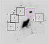 |
Fig. 2. Image of the full frame in the gF475W band with the region of PGC 087327, highlighted in magenta, and the four regions used as background frames in black. Each region is 1.1′ × 1.1′. The most conspicuous object in the center of this mosaic is NGC 3314A/B. |
Comparison of PGC 087327 and the background frames.
2.3. Modelling the galaxy
In order to improve GC detection in regions of the galaxy with high surface brightness, we subtracted the galaxy mean profile. We modelled the galaxy with elliptical isophotes using the Astropy affiliated package photutils (v1.0.2) in Python.
We first initialised a rough galaxy model using first-guess ellipticity and position angle parameters using the EllipseGeometry class in photutils. Then we initialised an object of the Ellipse class with the unmasked galaxy image data and this geometry, and performed a short and coarse fit using the fit_image routine within Ellipse. This provided us with a list of isophotes in the form of an object of the Isophote class, which were used to generate more refined starting parameters for the final fitting, which would be performed on the masked image.
To obtain the mask, we ran the sewpy wrapper3 for SExtractor (Bertin & Arnouts 1996), generating separate photometric catalogues of the extended and compact objects in the frame. At this stage of the selection, we only masked the brightest objects (mag < 24 for extended sources and mag < 25 for compact sources, in both passbands), and separated extended from compact sources using the SExtractor CLASS_STAR parameter (CLASS_STAR> 0.8 for compactness).
The final fit for elliptical isophotes was then performed on the masked image of PGC 087327 using the fit_image routine. A low-surface-brightness feature (possibly a diffuse foreground galaxy) and the bright star south-east of the core of PGC 087327, both visible in Fig. 1, were also masked out before running the isophotes fitting. The galaxy modelling run went out to a semi-major axis of 26.5″, where the galaxy surface brightness level reaches ≈26.3/26.0 mag arcsec−2 in the gF475W and VF606W bands, respectively. The model was synthesised from the list of isophotes generated by fit image using the build ellipse model function within Ellipse. Finally, the residuals were generated by subtracting the model from the original image of PGC 087327. Figure 3 shows the gF475W-band image of the galaxy and the smoothed residuals.
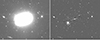 |
Fig. 3. Galaxy image and residuals. Left: PGC 087327 gF475W-band image. Right: galaxy-subtracted residual image. We further subtracted a smooth background map derived from SExtractor to improve the visibility of GC candidates near the galaxy center. The image size is 1.0′ × 0.85′. |
The isophote class also provides us with information on the total flux within each fitted elliptical isophote, which is stored in the variable ‘tflux_e’. Using a curve of growth analysis on the total flux within each isophote, we determine the total apparent magnitude of the galaxy in both gF475W and VF606W. The values of this analysis are quoted in Table 1.
We carried out an additional test with Galfit (Peng et al. 2010) in order to estimate the disc-to-bulge ratio using a combined fit of an elliptical and a Sersic component to the galaxy. We find that the B/T (bulge-to-total) ratio is 0.76, implying a D/B ≈ 0.32 (disc-to-bulge ratio). This, combined with the Sersic index of 5.8 from our Galfit run, puts PGC 087327 firmly in the E/S0 category (Baillard et al. 2011).
2.4. Source detection and photometry
Once we had the residual image, we re-ran SExtractor to generate the catalogue of sources in the image cutout. The catalogue was used to identify GCs in the frame.
The photometry of point-like sources was aperture and extinction-corrected as follows. We obtained the extinction correction from the IRSA (NASA/IPAC Infra-Red Science Archive) dust query module of Astropy, which gave us the value of EB − V at the position of our field(s). The value of RV was adopted from Schlafly & Finkbeiner (2011). The aperture correction values were obtained from the instrument webpages, using the online encircled energy plots4, where the encircled energy is the fraction of flux contained within a certain radius of aperture (Sirianni et al. 2005). We chose an aperture radius of r = 0.12″, which corresponds approximately to the FWHM (full-width at half-maximum) of our data (see Table 2).
We verified the adopted encircled energy values by obtaining the aperture correction from the analysis of the most isolated, compact, and bright objects in the field. By inspecting the curve of growth (i.e. the aperture magnitude at different radii) out to 64 pixels aperture, we obtained aperture correction values that agree within ±0.04 mag with the ones from the HST/ACS calibration team. We finally matched the aperture-and-extinction-corrected catalogues across the gF475W and VF606W bands, using a matching radius of 3 pixels (∼0.12″). This was done in order to select only the sources that appear in both bands. The same procedure for the photometry, extinction, and aperture corrections as well as a cross-matching was also applied to the four background fields.
The full catalogue of GC candidates identified in the galaxy field is available in Table A.2. In the catalogue we provide the positions (Cols. 2 and 3), the aperture-and-extinction-corrected magnitudes with errors for the gF475W and VF606W bands (Cols. 4–7), the gF475W − VF606W colour, and the flux radius (half-light radius from SExtractor) Frad and FWHM in each band (Cols. 9–12) for the sample of selected GCs.
3. Globular cluster population: Sample selection
In this section we describe the procedures adopted to identify GC candidates from the cross-matched catalogue derived in the previous section. Since GCs at the distance of the Hydra I appear as point-like objects (1″ corresponds to nearly 100 pc), it is reasonable to identify them by means of their shape, in addition to their photometric properties. We selected GCs using three criteria based on their i) compactness, ii) colour, and iii) magnitude. The same selection procedure was applied to the catalogues of the four background fields.
3.1. Compactness
The selection on compactness was used to separate the compact GC candidates from the extended sources. We identified compact sources using the SExtractor CLASS_STAR parameter and the concentration index (CI).
For the SExtractor star-galaxy separation parameter CLASS_STAR, which has a value close to 1.0 for compact objects, we adopted a threshold value of CLASS_STAR ≥ 0.8. The CI is defined as the difference between magnitudes at two different apertures, and is a further indicator of source compactness (Peng et al. 2011). After several tests, we set the two aperture diameters at 4 and 8 pixels to calculate CI = mag4pix − mag8pix. We then selected all sources with 0.25 ≤ CI ≤ 0.75 in both passbands, based on the median and scatter of the sequence of compact sources in the CI versus magnitude plot. The selection of compact sources is shown in Fig. 4 with black points.
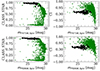 |
Fig. 4. Identification of GC candidates using compactness. Left: star-galaxy classifier of all detected sources in the matched catalogue (green) and GC candidates (black). Right: concentration indices for all the detected sources in the matched catalogue (green) and GC candidates (black). |
3.2. Colour and magnitudes
The selection based on colour enables us to reduce the contamination from fore- and background compact sources in the field, mostly Milky Way stars and distant galaxies, respectively. Figure 5 shows the colour-magnitude diagrams of sources detected in PGC 087327 and in the four reference fields. The upper left panel of the figure shows the colour-magnitude diagram of the entire sample of matched sources with no selection. The panel reveals the presence of a sharp drop in the number of detected sources having a gF475W − VF606W colour bluer than ∼0.3 and redder than ∼0.7 mag, which is not seen in the four background fields, shown in the other panels of the figure.
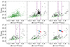 |
Fig. 5. Colour-magnitude diagram of all objects detected (green; top left), along with the objects selected by compactness criteria (black) in the PGC 087327 frame (top center), and background reference frames (all others). The GC candidates are the compact objects (black) within the colour interval marked by purple dashed vertical lines in all panels. The bottom two panels also show the SPoT (bottom left panel) and YEPS (bottom right panel) SSP models (with an arbitrary magnitude shift) overlaid on top of the colour-magnitude plots for regions 3 and 4. Different SSP [Fe/H] are shown with different colours : −2.5 ≤ [Fe/H] ≤ − 1.5 in orange, −1.5 < [Fe/H] ≤ 0 in blue, and 0 < [Fe/H] ≤ 0.5 in red. The vertical dotted lines in the middle panel show the colour interval adopted for GC selection. |
Intermediate-size galaxies such as PGC 087327 typically do not contain a substantial population of red, metal-rich GCs (Peng et al. 2006). Using an updated version of the Stellar POpulations Tools (SPoT, Raimondo et al. 2005) simple stellar population (SSP) models, we estimate that with [Fe/H] ≤ 0, and age ≥ 10 Gyr, the range of colour we expect for GCs is conservatively 0.3 ≤ ⟨gF475W − VF606W⟩≤0.7 mag. We used this colour range from SSP models, combined with the properties observed in the colour-magnitude diagrams in Fig. 5, to select the GC candidates in our catalogue. A similar range of GC colours was corroborated by examining the Yonsei Evolutionary Population Synthesis (YEPS, Chung et al. 2020) SSP models5. The SPoT models are reported in Table A.1.
After the compactness and colour selections from the matched catalogues, we also applied a cut on the magnitude. As anticipated in Sect. 1, the GCLF has a universal Gaussian shape and a width σGCLF, which scales with the galaxy luminosity. Using Eq. (5) from Villegas et al. (2010) and adopting a total galaxy magnitude Mz, gal ∼ −20.4 mag (see Table 1), we evaluated  mag. Adopting a preliminary value of
  mag (we refine this in Sect. 4.4) and a distance of 61 Mpc, we estimated the expected GCLF peak
  mag. We selected from the matched catalogue all sources
  around the
  , using a large interval in order to avoid introducing bias in our own distance estimate.
A synthesis of the GC candidates identified in PGC 087327 and the background fields is also given in Table 3. Figure 5 shows the sources identified as GC candidates in the colour-magnitude diagram. The plots and data in Table 3 show that the galaxy hosts a factor of ∼5 more GCs than the background fields. From Fig. 5, we can verify that the number of objects selected through the compactness criteria with colours bluer than the GC colour, ⟨gF475W − VF606W⟩< 0.3, have a similar density in the PGC 087327 frame (Nred, gal = 35) as in the background frames (median Nred, bkg = 35 ± 9). A similar trend is also observed in the population of objects redder than the GCs colour, ⟨gF475W − VF606W⟩> 0.7 (Nblue, gal = 15, median Nblue, bkg = 14 ± 2). The last two panels in the figure also show the colours and magnitudes from the SPoT and YEPS SSP models, with a magnitude offset factored in to match the magnitude range in the plots.
In summary, even though the GC selection is based on a single colour and shape criterion, the plots in Fig. 5 reveal a significant over-density of GC candidates in the galaxy frame compared to the background fields. In the next section, we take advantage of that to characterise the GC population.
Some of the objects in the GC candidate catalogue have a larger than average flux radius, with SExtractor half-light radii Frad ≳ 2 pix (compared to the median Frad = 1.7 pix), relatively red colours (⟨gF475W − VF606W⟩> 0.53 mag), and magnitude MF606W ≈ −7.1 mag, which make them probable candidates for ’faint fuzzies’, which have historically been observed with similar characteristics close to many lenticular galaxies (Brodie & Strader 2006).
4. Globular cluster population analysis
4.1. Colour distribution
Despite the small separation in wavelength between the gF475W and VF606W passbands, the colour histogram of the selected GCs shows a clear bimodality. By inspecting the entire population of matched sources on PGC 087327 and in the reference fields, it is hard to identify any evidence of this feature (Fig. 6, left panel). However, the bimodality emerges when the colour distribution of GC candidates is inspected, and it is especially evident when we subtract the background obtained from the four reference frames (Fig. 6, middle and right panels).
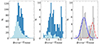 |
Fig. 6. Colour histograms of the full matched sample (left panel) and of the GC candidates (center) as well as the colour distribution of GCs over PGC 087327 corrected for the background contamination (right). The light blue histograms in the left and central panels indicate mean colour distributions in the background frames, and the dark blue histograms represent the distribution in the frame of PGC 087327. In the right panel the Gaussian fits (from GMM) for the blue (solid blue line) and red (dot-dashed red line) GC sub-populations are overlaid on the background-corrected colour density histogram. |
To study the detailed properties of the colour distribution, we generated a random sample of ∼1000 points in the shape of the background-subtracted histogram of GCs (Fig. 6, right panel), using the numpy routine random.choice. In order to make this distribution more continuous, each bin in this histogram of random points was smoothed with a uniform distribution having a width equal to half of the bin size. The resulting distribution, exhibiting a dual Gaussian profile, was fitted using Gaussian Mixture Models (GMM, Muratov & Gnedin 2010), repeated over ten iterations. We found that a bimodal distribution is favored over a unimodal one, and the median blue (red) peak of the background subtracted density distribution lies at ⟨gF475W − VF606W⟩ = 0.47 (0.62) mag, with a width of 0.05 (0.03) mag. The resulting fraction of red GCs is fred ∼ 0.3 ± 0.1, which agrees with the median value of fred ∼ 0.18 ± 0.20 from Peng et al. (2008, their Table 3) for galaxies similar to PGC 087327, with a specific frequency (SN) between 1.0 and 2.5 (further discussed in Sect. 4.4).
Due to the lack of existing literature on the bimodality in gF475W − VF606W colour, we projected the gF475W − VF606W peaks to V − I and g − z colours, using the SpoT and Yonsei models for the transformation. Considering an interval of ⟨gF475W − VF606W⟩±0.05 mag around each peak and adopting predictions for ages t ≥ 10 Gyr and metallicity −2.5 ≤ [Fe/H] ≤ 0, we found that the blue gF475W − VF606W = 0.47 mag peak projects into V − I = 0.55 mag and g − z = 0.93 mag, while the red gF475W − VF606W = 0.62 mag peak is projected into V − I = 0.78 mag and g − z = 1.34 mag. We compared the projected colours for each peak with the values from the review by Brodie & Strader (2006, their Table 1), for galaxies similar to PGC 087327, having type S0 and −19.5 ≤ MB ≤ −17.5 mag. The median colours from this selection are ⟨V − I⟩ = 0.51 (0.72) mag and ⟨g − z⟩ = 0.92 (1.26) mag for the blue (red) peak, which agree with our results within ∼0.1 mag. In summary, despite the narrow wavelength interval available, the GCs colour bimodality appears to be consistent with the results obtained for similar galaxies over a wider wavelength range.
4.2. Radial distribution
The coordinates of the GCs identified in each frame were plotted to understand the radial distribution of the sources in the frame of PGC 087327 (Fig. 7). The GCs were separated into two different classes based on their ⟨gF475W − VF606W⟩ colour: red (⟨gF475W − VF606W⟩≥0.53, adopted from GMM fits) and blue (⟨gF475W − VF606W⟩< 0.53). From Fig. 7 (left panel) and Fig. 8 we can identify that red, more metal-rich GCs appear clustered near the center of the galaxy compared to the blue. The slope of the radial number density of the red GCs is steeper ( ) than the blue (αb ≈ −1.7). The slopes agree with the values of the slopes for metal-rich and metal-poor subpopulations quoted by Brodie & Strader (2006). We also plotted the galaxy surface brightness radial profile (scaled appropriately), to emphasise its resemblance to the radial density profile of the red GCs. Around a radius of ∼32″ we begin to approach the edges of the galaxy cutout, and to avoid issues due to vignetting we do not consider this region for our fits (indicated by grey shaded area in Fig. 8). In Fig. 7 we have plotted the kernel density estimate plots for the red and blue sub-populations, and we calculated that the ellipticity of the red GCs (center frame) is ϵ = 0.41, where ϵ is the ratio of the minor to the major axis. The ϵ for red GCs matches that of our model isophotes in Sect. 2.3. The KDE plot of the blue sub-population, on the other hand, has a more circular distribution with ϵ = 0.13 and a higher variation at larger radii.
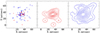 |
Fig. 7. Spatial distribution of the GC candidates divided into red and blue according to colour (⟨gF475W − VF606W⟩≥0.53 is red) in the frame of PGC 087327 (left) and the KDE plot of the blue (center) and red (right) GC sub-populations. |
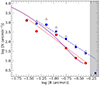 |
Fig. 8. Radial densities of the full (black triangles), red (red circles), and blue (blue squares) GC populations in PGC 087327. The radial density profile for the red (dashed line) and blue (dot-dashed line) GC populations is also shown as a linear trend. The radial surface brightness profile of the galaxy (scaled appropriately) is shown with the purple solid line. The shaded grey region shows the limit of geometric completeness as we approach the margins of our image cutout. |
4.3. Luminosity function
The histograms of GCs in the frame of PGC 087327 and the background frames were inspected to study the luminosity function. As for the colour and radial distribution, we used the four reference fields to define the background level of contaminant sources to be subtracted from the GC density over PGC 087327. Since the area of the background fields is the same as the cutout of PGC 087327, it is not necessary to normalise to the area to properly subtract the background contamination. Figure 9 shows the luminosity function of the sources detected in PGC 087327 and (the mean) of the reference regions for the full matched catalogues. The middle panel of the same figure shows the luminosity functions for the GC candidates. As expected, the GCs on-galaxy significantly outnumber the counts in the reference fields. We also note a slight increase in background counts towards fainter magnitudes, as an effect of the lower efficiency of the adopted selection criteria for sources with lower S/N. The background -subtracted luminosity function of GCs is shown in Fig. 9 (right panel). In order to use the GCLF for deriving the distance modulus of PGC 087327, it must be corrected for completeness first.
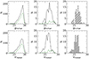 |
Fig. 9. Luminosity functions. Left: luminosity function (LF) of all detected and matched objects in the frame of PGC 087327 (in black), and in the background fields (in green, dashed). Center: LF of the GC candidates in the galaxy frame (in black), and the mean LF of GC candidates over the four background fields (in green). Right: LF of the GC candidates in PGC 087327 after subtracting the mean LF from the background fields. This luminosity function has not yet been corrected for completeness. |
The completeness function in each band was determined by injecting and then detecting a total of ∼850 artificial stars on the gF475W and VF606W residual frames. At first, we derived a point spread function (PSF) from the bright, compact, and isolated sources in the image in each band. The brightest and most isolated compact sources were extracted from the residual image using the extract stars routine of Astropy, and these extracted stars were then fed into the EPSFBuilder routine of the photutils package to generate an effective PSF of the size 41 × 41 pixels. The magnitudes of artificial stars to be injected were obtained by generating a random sample of magnitudes, again using numpy.random.choice, in the shape of the histogram of all sources detected in the galaxy frame, limited to the range 23 ≤ mag ≤ 32. These stars were injected in the residual frame of PGC 087327 along an equispaced grid whose position was varied over 50 iterations. A catalogue of detected sources was obtained from a run of SExtractor on this synthesised image, adopting the same parameters used for generating the GC catalogue. The aperture correction for each band was then applied to this catalogue. A twofold selection algorithm was used to match the detected to the injected artificial stars: a first selection on separation (≤6 pix), followed by a cut on the magnitude difference (absolute difference |minjected − mdetected|≤0.5 mag). The ratio of the number of sources thus retrieved versus injected, in each magnitude bin, gives us the discrete completeness function (Fig. 10).
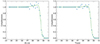 |
Fig. 10. Completeness functions in gF475W (left) and VF606W (right). Each point represents the ratio of the number of sources detected vs. injected, in each magnitude bin, and the green line shows the best fit modified Fermi function. |
We fitted the completeness function with a modified Fermi function (Alamo-Martínez et al. 2013, their Eq. (2)), and interpolated it to counteract the discrete nature of the sampled magnitudes, then applied it to correct the GCLF in the galaxy frame. We note that the completeness is 90% down to about m ≈ 29.5 in both gF475W and VF606W, which is fainter than the 3σGCLF tail of the galaxy mTO. In other words, the observed GCLF is complete and only mildly affected by the completeness, and a correction of ∼5% is required for magnitudes gF475W = 28 − 29 mag. The same analysis was performed on the background frames to determine their completeness functions individually, and the mean of the completeness-corrected luminosity functions of GC candidates from the four background frames was used to determine and subtract the overall background for the GCLF in PGC 087327.
Finally, the background-subtracted GCLF was fitted with a Gaussian in both the gF475W and VF606W bands (Fig. 11) to obtain the peak turnover apparent magnitude and the width. The results of the fit are given in Table 4.
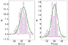 |
Fig. 11. Final GCLF which has been corrected for completeness, and fitted with a Gaussian (green line). |
GCLF parameters.
4.4. GCLF distance: Calibration and results
In order to derive the GCLF distance to PGC 087327, we adopted the apparent mTO derived as described in Sect 4.3 combined with MTO calibrations in gF475W and VF606W from the literature. The details of the calibration are outlined below.
We estimated the absolute VF606W band turnover by taking advantage of the existing accurate GCLF analysis by Georgiev et al. (2009) on HST/ACS data of dwarf galaxies. We used their calibration quoted in the V band, which gives us  mag. Using the photometric transformation in Table 21 from Sirianni et al. (2005) and inverting the relation given in Eq. (12), we find the
  :
:

The colour used in this equation is the V − I colour of GCs, which is ∼1 (Harris 1996; Cantiello et al. 2007), and ZptF606W(AB) is the zero-point magnitude of the F606W band (Table 2) for the date of our observation, obtained from the zero-point calculator of the HST/ACS6. Performing this analysis for the observed and synthetic (colour > 0.4) coefficients in Sirianni et al. (2005), we find two individual estimates:  mag and
  mag. On averaging these two values, we get
  mag.
mag.
To obtain the gF475W band MTO, we used the ACS Virgo Cluster Survey (ACSVCS) results. We isolated a sub-sample of galaxies with −19 ≤ MB (mag)≤ − 17, which corresponds to the magnitude level of PGC 087327 (see Table 1). From this sample, we excluded the galaxies with a number of GCs NGC < 30, as well as VCC 1025 (since it belongs to the W’ cloud and has a different distance modulus). We calculated the median turnover magnitude of the selected sub-sample and the rms (derived from the median absolute deviation), which turns out to be  mag. Adopting (m − M)SBF = 31.09 ± 0.15 for the Virgo cluster from Blakeslee et al. (2009), we find :

We calculated the distance modulus mTO − MTO in each band, the results of which are in Table 4. Being independent measurements (except the catalogues were cleaned by matching the gF475W and VF606W photometry), we assume our best distance modulus to PGC 087327 to be the weighted average of the two values in Table 4: (m − M)GCLF = 33.77 ± 0.17 mag, or 56.7 ± 4.3 Mpc. This agrees with the distance estimate from the fundamental plane for this galaxy, (m − M) = 33.8 ± 0.5 mag (Tully et al. 2013).
The systematic error on the calibrations derived above could be assumed to be of the same order of the Surface Brightness Fluctuations (SBF) method systematic, in other words,∼0.1 mag (Cantiello et al. 2018). Lee et al. (2018) claim that the real global systematic for GCLF is < 0.3 mag. We adopt a conservative middle-ground estimate of 0.2 mag as our systematic error budget. Hence, including systematic errors, we obtain DGCLF = 56.7 ± 4.3(statistical)±5.2(systematic) Mpc.
We estimated the value of the Hubble parameter using the flow-corrected radial velocity for PGC 087327 from Table 4. Combining it with the distance modulus from this work, we find H0 ≈ 78.5 ± 6.0(statistical)±7.3(systematic) km s−1 Mpc−1.
The distance modulus from this work places PGC 087327 between NGC 3314A ((m − M) = 33.19 ± 0.40 mag, from Theureau et al. 2007) and NGC 3314B ((m − M) = 34.37 ± 0.15 mag, from Mould et al. 2000) in projection, consistent with other distance measurements for the Hydra cluster and lying close to the upper end of these estimates (e.g., Blakeslee et al. 2002; Hudson et al. 2004; Mieske et al. 2005). Our results show that this galaxy lies at a distance that is ∼20% larger than that of the two BCGs in the Hydra I cluster (Tully et al. 2013), and in a region where we count eight other brighter galaxies that have up to 20% larger velocity distances than that of PGC 087327 in the vicinity of ∼15′7.
Considering the Hubble-Lemaitre distance to PGC 087327 and the results in Table 4, we can turn the argument around and use our results to check whether the fitted parameters support the universality of the GCLF. Given the fact that the final distance calculated in our work agrees closely with the velocity distance (reported in Table 1), combined with the σGCLF values from our analysis that match very well with the expected σGCLF = 0.93 mag (see Sect. 3.2), we can conclude that the results from this work support the universality of the GCLF method.
4.5. Specific frequency
We can also estimate the specific frequency (Harris & van den Bergh 1981) of the GC system in PGC 087327, which is defined as:
Using the mF606W, gal obtained from our fit in Sect. 2.3 (quoted in Table 1), correcting it for extinction and using Table 21 from Sirianni et al. (2005), we transform mF606W, gal to mV, gal in Vegamag, which is used as a reference for SN estimates. Combining this apparent magnitude with the distance modulus of PGC 087327 (from Sect. 4.4), we estimate a specific frequency SN = 1.8 ± 0.7. The value we estimated is consistent with the observed scatter of SN for galaxies of similar magnitude (Peng et al. 2008; Harris et al. 2013), leaning towards the tail of higher GC population density.
5. Conclusions
In this work, we benefited from extremely deep images in the HST/ACS gF475W and VF606W bands to characterise the GC population around PGC 087327. The main results of our study are summarised below:
-
Although the population of GCs we find is relatively small, NGC = 82 ± 9, and the wavelengths of the gF475W and VF606W bands are relatively close, we find a clear bimodal colour distribution in the GC system of this galaxy.
-
The radial distribution of the GCs shows a clustering of the red GCs close to the core of the galaxy, which falls off rapidly at higher radii (αr ≈ −1.9) and has a close resemblance to the galaxy surface brightness profile, whereas the blue GCs are less concentrated at the center, taper off more slowly away from the galaxy core (αb ≈ −1.7), and appear circularly distributed around the galaxy.
-
In spite of the close wavelengths of the gF475W and VF606W bands, and the intermediate-mass of PGC 087327, we observe the typical bimodal characteristics of GC populations that are more pronounced in massive galaxies. The gF475W–VF606W colour distribution shows a blue (red) peak at ⟨gF475W − VF606W⟩ = 0.47(0.62). This further demonstrates the role of the quality of the images on the characterization of GC populations, since a lower depth and accuracy of images would have smeared out the colour bimodality feature we observe in this work.
-
The turnover magnitudes in gF475W and VF606W are both ∼3 mag brighter than the completeness limit (> 29.5 mag), which to our knowledge is an unprecedented finding at distances of the order of 60 Mpc.
-
We estimate a distance modulus of (m − M) = 33.77 ± 0.17 mag, or 56.7 ± 4.3(statistical) Mpc for this galaxy, which places it between NGC 3314A and NGC 3314B in projection.
-
Considering the velocity distance of PGC 087327 and the empirical expectations for the GCLF peak and width, our analysis for this target supports the universality of the GCLF method.
-
Assuming ∼10% systematic error on the galaxy distance, we derive a Hubble constant value of H0 ≈ 78.5 ± 6.0 (statistical)±7.3 (systematic) km s−1 Mpc−1.
Throughout this work, we always consider the ABmag photometric system, unless specified otherwise.
The YEPS models can be found on http://cosmic.yonsei.ac.kr/YEPS.htm
Can be found at the URL: https://acszeropoints.stsci.edu/
Source: Nasa Extragalatic Database.
Acknowledgments
This work was carried out based on observations made with the NASA/ESA Hubble Space Telescope, and obtained from the Hubble Legacy Archive, which is a collaboration between the Space Telescope Science Institute (STScI/NASA), the Space Telescope European Coordinating Facility (ST-ECF/ESA) and the Canadian Astronomy Data Center (CADC/NRC/CSA). The authors made use of Astropy (http://www.astropy.org), a community-developed core Python package for Astronomy (Astropy Collaboration 2013, 2018), along with the databases of HyperLeda (Makarov et al. 2014), the Extragalactic Distance Database (EDD, https://edd.ifa.hawaii.edu/) and the NASA/IPAC Extragalactic Database (NED, which is operated by the Jet Propulsion Laboratory, California Institute of Technology, under contract with the National Aeronautics and Space Administration). We also made extensive use of the softwares of Topcat (http://www.starlink.ac.uk/topcat/), SExtractor (Bertin & Arnouts 1996) and Galfit (Peng et al. 2010). M.C. acknowledges support from MIUR, PRIN 2017 (grant 20179ZF5KS). The authors would also like to acknowledge and thank the referee for their valuable comments, questions and suggestions.
References
- Alamo-Martínez, K. A., Blakeslee, J. P., Jee, M. J., et al. 2013, ApJ, 775, 20 [CrossRef] [Google Scholar]
- Astropy Collaboration (Robitaille, T. P., et al.) 2013, A&A, 558, A33 [NASA ADS] [CrossRef] [EDP Sciences] [Google Scholar]
- Astropy Collaboration (Price-Whelan, A. M., et al.) 2018, AJ, 156, 123 [Google Scholar]
- Baillard, A., Bertin, E., de Lapparent, V., et al. 2011, A&A, 532, A74 [NASA ADS] [CrossRef] [EDP Sciences] [Google Scholar]
- Bassino, L. P., & Caso, J. P. 2017, MNRAS, 466, 4259 [NASA ADS] [Google Scholar]
- Beasley, M. A., & Sharples, R. M. 2000, MNRAS, 311, 673 [NASA ADS] [CrossRef] [Google Scholar]
- Bernardi, M., Alonso, M. V., da Costa, L. N., et al. 2002, AJ, 123, 2990 [NASA ADS] [CrossRef] [Google Scholar]
- Bertin, E., & Arnouts, S. 1996, A&AS, 117, 393 [NASA ADS] [CrossRef] [EDP Sciences] [Google Scholar]
- Blakeslee, J. P., Lucey, J. R., Tonry, J. L., et al. 2002, MNRAS, 330, 443 [Google Scholar]
- Blakeslee, J. P., Jordán, A., Mei, S., et al. 2009, ApJ, 694, 556 [Google Scholar]
- Blakeslee, J. P., Jensen, J. B., Ma, C.-P., Milne, P. A., & Greene, J. E. 2021, ApJ, 911, 65 [NASA ADS] [CrossRef] [Google Scholar]
- Bohlin, R. C. 2016, AJ, 152, 60 [NASA ADS] [CrossRef] [Google Scholar]
- Brodie, J. P., & Strader, J. 2006, ARA&A, 44, 193 [Google Scholar]
- Cantiello, M., & Blakeslee, J. P. 2007, ApJ, 669, 982 [NASA ADS] [CrossRef] [Google Scholar]
- Cantiello, M., & Blakeslee, J. P. 2012, Mem. Soc. Astron. It. Suppl., 19, 184 [Google Scholar]
- Cantiello, M., Blakeslee, J. P., & Raimondo, G. 2007, ApJ, 668, 209 [NASA ADS] [CrossRef] [Google Scholar]
- Cantiello, M., Jensen, J. B., Blakeslee, J. P., et al. 2018, ApJ, 854, L31 [Google Scholar]
- Cappellari, M. 2013, ApJ, 778, L2 [NASA ADS] [CrossRef] [Google Scholar]
- Carretta, E., Gratton, R. G., Clementini, G., & Pecci, F. F. 2000, ApJ, 533, 215 [Google Scholar]
- Chung, C., Yoon, S.-J., Cho, H., Lee, S.-Y., & Lee, Y.-W. 2020, ApJS, 250, 33 [NASA ADS] [CrossRef] [Google Scholar]
- Cohen, J. G., Blakeslee, J. P., & Ryzhov, A. 1998, ApJ, 496, 808 [NASA ADS] [CrossRef] [Google Scholar]
- Ferrarese, L., Mould, J. R., Kennicutt, R. C., et al. 2000, ApJ, 529, 745 [NASA ADS] [CrossRef] [Google Scholar]
- Forbes, D. A., Spitler, L. R., Strader, J., et al. 2011, MNRAS, 413, 2943 [NASA ADS] [CrossRef] [Google Scholar]
- Georgiev, I. Y., Puzia, T. H., Hilker, M., & Goudfrooij, P. 2009, MNRAS, 392, 879 [NASA ADS] [CrossRef] [Google Scholar]
- Goudfrooij, P., Mack, J., Kissler-Patig, M., Meylan, G., & Minniti, D. 2001, MNRAS, 322, 643 [NASA ADS] [CrossRef] [Google Scholar]
- Hanes, D. A. 1977, MNRAS, 180, 309 [Google Scholar]
- Harris, W. E. 1996, AJ, 112, 1487 [Google Scholar]
- Harris, W. E. 2009, ApJ, 703, 939 [NASA ADS] [CrossRef] [Google Scholar]
- Harris, W. E., & van den Bergh, S. 1981, AJ, 86, 1627 [NASA ADS] [CrossRef] [Google Scholar]
- Harris, W. E., Harris, G. L. H., & Alessi, M. 2013, ApJ, 772, 82 [Google Scholar]
- Hudson, M. J., Smith, R. J., Lucey, J. R., & Branchini, E. 2004, MNRAS, 352, 61 [Google Scholar]
- Into, T., & Portinari, L. 2013, MNRAS, 430, 2715 [Google Scholar]
- Khetan, N., Izzo, L., Branchesi, M., et al. 2021, A&A, 647, A72 [NASA ADS] [CrossRef] [EDP Sciences] [Google Scholar]
- Kuntschner, H., Ziegler, B. L., Sharples, R. M., Worthey, G., & Fricke, K. J. 2002, A&A, 395, 761 [NASA ADS] [CrossRef] [EDP Sciences] [Google Scholar]
- Lee, B., & Chary, R.-R. 2020, MNRAS, 497, 1935 [NASA ADS] [CrossRef] [Google Scholar]
- Lee, M. G., Kang, J., & Im, M. 2018, ApJ, 859, L6 [NASA ADS] [CrossRef] [Google Scholar]
- Makarov, D., Prugniel, P., Terekhova, N., Courtois, H., & Vauglin, I. 2014, A&A, 570, A13 [NASA ADS] [CrossRef] [EDP Sciences] [Google Scholar]
- Mieske, S., Hilker, M., & Infante, L. 2005, A&A, 438, 103 [NASA ADS] [CrossRef] [EDP Sciences] [Google Scholar]
- Mould, J. R., Huchra, J. P., Freedman, W. L., et al. 2000, ApJ, 529, 786 [Google Scholar]
- Muratov, A. L., & Gnedin, O. Y. 2010, ApJ, 718, 1266 [Google Scholar]
- Peng, E. W., Jordán, A., Côté, P., et al. 2006, ApJ, 639, 95 [Google Scholar]
- Peng, E. W., Jordán, A., Côté, P., et al. 2008, ApJ, 681, 197 [NASA ADS] [CrossRef] [Google Scholar]
- Peng, C. Y., Ho, L. C., Impey, C. D., & Rix, H.-W. 2010, AJ, 139, 2097 [Google Scholar]
- Peng, E. W., Ferguson, H. C., Goudfrooij, P., et al. 2011, ApJ, 730, 23 [Google Scholar]
- Raimondo, G., Brocato, E., Cantiello, M., & Capaccioli, M. 2005, AJ, 130, 2625 [Google Scholar]
- Richtler, T. 2006, Bull. Astron. Soc. India, 34, 83 [NASA ADS] [Google Scholar]
- Schlafly, E. F., & Finkbeiner, D. P. 2011, ApJ, 737, 103 [Google Scholar]
- Sirianni, M., Jee, M. J., Benítez, N., et al. 2005, PASP, 117, 1049 [Google Scholar]
- Smith, R. J., Lucey, J. R., Hudson, M. J., Schlegel, D. J., & Davies, R. L. 2000, MNRAS, 313, 469 [NASA ADS] [CrossRef] [Google Scholar]
- Theureau, G., Hanski, M. O., Coudreau, N., Hallet, N., & Martin, J. M. 2007, A&A, 465, 71 [NASA ADS] [CrossRef] [EDP Sciences] [Google Scholar]
- Tonry, J. L., Dressler, A., Blakeslee, J. P., et al. 2001, ApJ, 546, 681 [Google Scholar]
- Tully, R. B., Courtois, H. M., Dolphin, A. E., et al. 2013, AJ, 146, 86 [NASA ADS] [CrossRef] [Google Scholar]
- Tully, R. B., Courtois, H. M., & Sorce, J. G. 2016, AJ, 152, 50 [Google Scholar]
- Villegas, D., Jordán, A., Peng, E. W., et al. 2010, ApJ, 717, 603 [Google Scholar]
- Yoon, S.-J., Yi, S. K., & Lee, Y.-W. 2006, Science, 311, 1129 [Google Scholar]
Appendix A: Tables
SPoT models
GC catalog
All Tables
All Figures
|
Fig. 1. Colour composite 2′ × 1′ HST image of PGC 087327. North is up and east is left. |
| In the text | |
|
Fig. 2. Image of the full frame in the gF475W band with the region of PGC 087327, highlighted in magenta, and the four regions used as background frames in black. Each region is 1.1′ × 1.1′. The most conspicuous object in the center of this mosaic is NGC 3314A/B. |
| In the text | |
|
Fig. 3. Galaxy image and residuals. Left: PGC 087327 gF475W-band image. Right: galaxy-subtracted residual image. We further subtracted a smooth background map derived from SExtractor to improve the visibility of GC candidates near the galaxy center. The image size is 1.0′ × 0.85′. |
| In the text | |
|
Fig. 4. Identification of GC candidates using compactness. Left: star-galaxy classifier of all detected sources in the matched catalogue (green) and GC candidates (black). Right: concentration indices for all the detected sources in the matched catalogue (green) and GC candidates (black). |
| In the text | |
|
Fig. 5. Colour-magnitude diagram of all objects detected (green; top left), along with the objects selected by compactness criteria (black) in the PGC 087327 frame (top center), and background reference frames (all others). The GC candidates are the compact objects (black) within the colour interval marked by purple dashed vertical lines in all panels. The bottom two panels also show the SPoT (bottom left panel) and YEPS (bottom right panel) SSP models (with an arbitrary magnitude shift) overlaid on top of the colour-magnitude plots for regions 3 and 4. Different SSP [Fe/H] are shown with different colours : −2.5 ≤ [Fe/H] ≤ − 1.5 in orange, −1.5 < [Fe/H] ≤ 0 in blue, and 0 < [Fe/H] ≤ 0.5 in red. The vertical dotted lines in the middle panel show the colour interval adopted for GC selection. |
| In the text | |
|
Fig. 6. Colour histograms of the full matched sample (left panel) and of the GC candidates (center) as well as the colour distribution of GCs over PGC 087327 corrected for the background contamination (right). The light blue histograms in the left and central panels indicate mean colour distributions in the background frames, and the dark blue histograms represent the distribution in the frame of PGC 087327. In the right panel the Gaussian fits (from GMM) for the blue (solid blue line) and red (dot-dashed red line) GC sub-populations are overlaid on the background-corrected colour density histogram. |
| In the text | |
|
Fig. 7. Spatial distribution of the GC candidates divided into red and blue according to colour (⟨gF475W − VF606W⟩≥0.53 is red) in the frame of PGC 087327 (left) and the KDE plot of the blue (center) and red (right) GC sub-populations. |
| In the text | |
|
Fig. 8. Radial densities of the full (black triangles), red (red circles), and blue (blue squares) GC populations in PGC 087327. The radial density profile for the red (dashed line) and blue (dot-dashed line) GC populations is also shown as a linear trend. The radial surface brightness profile of the galaxy (scaled appropriately) is shown with the purple solid line. The shaded grey region shows the limit of geometric completeness as we approach the margins of our image cutout. |
| In the text | |
|
Fig. 9. Luminosity functions. Left: luminosity function (LF) of all detected and matched objects in the frame of PGC 087327 (in black), and in the background fields (in green, dashed). Center: LF of the GC candidates in the galaxy frame (in black), and the mean LF of GC candidates over the four background fields (in green). Right: LF of the GC candidates in PGC 087327 after subtracting the mean LF from the background fields. This luminosity function has not yet been corrected for completeness. |
| In the text | |
|
Fig. 10. Completeness functions in gF475W (left) and VF606W (right). Each point represents the ratio of the number of sources detected vs. injected, in each magnitude bin, and the green line shows the best fit modified Fermi function. |
| In the text | |
|
Fig. 11. Final GCLF which has been corrected for completeness, and fitted with a Gaussian (green line). |
| In the text | |
Current usage metrics show cumulative count of Article Views (full-text article views including HTML views, PDF and ePub downloads, according to the available data) and Abstracts Views on Vision4Press platform.
Data correspond to usage on the plateform after 2015. The current usage metrics is available 48-96 hours after online publication and is updated daily on week days.
Initial download of the metrics may take a while.