| Issue |
A&A
Volume 666, October 2022
|
|
|---|---|---|
| Article Number | A14 | |
| Number of page(s) | 23 | |
| Section | Extragalactic astronomy | |
| DOI | https://doi.org/10.1051/0004-6361/202243367 | |
| Published online | 29 September 2022 | |
Are the host galaxies of long gamma-ray bursts more compact than star-forming galaxies of the field?
1
Université Paris-Saclay, Université Paris Cité, CEA, CNRS, AIM, 91191 Gif-sur-Yvette, France
e-mail: benjamin.schneider@cea.fr
2
Excellence Cluster ORIGINS, Boltzmannstraße 2, 85748 Garching, Germany
3
Ludwig-Maximilians-Universität, Schellingstraße 4, 80799 München, Germany
4
GEPI, Observatoire de Paris, PSL University, CNRS, 5 Place Jules Janssen, 92190 Meudon, France
Received:
18
February
2022
Accepted:
27
June
2022
Context. Long gamma-ray bursts (GRBs) offer a promising tool for tracing the cosmic history of star formation, especially at high redshift, where conventional methods are known to suffer from intrinsic biases. Previous studies of GRB host galaxies at low redshift showed that high surface density of stellar mass and high surface density of star formation rate (SFR) can potentially enhance the GRB production. Evaluating the effect of such stellar densities at high redshift is therefore crucial to fully control the ability of long GRBs for probing the activity of star formation in the distant Universe.
Aims. We assess how the size, stellar mass, and star formation rate surface densities of distant galaxies affect the probability of their hosting a long GRB, using a sample of GRB hosts at z > 1 and a control sample of star-forming sources from the field.
Methods. We gathered a sample of 45 GRB host galaxies at 1 < z < 3.1 observed with the Hubble Space Telescope WFC3 camera in the near-infrared. Our subsample at 1 < z < 2 has cumulative distributions of redshift and stellar mass consistent with the host galaxies of known unbiased GRB samples, while our GRB host selection at 2 < z < 3.1 has lower statistics and is probably biased toward the high end of the stellar mass function. Using the GALFIT parametric approach, we modeled the GRB host light profile with a Sérsic component and derived the half-light radius for 35 GRB hosts, which we used to estimate the star formation rate and stellar mass surface densities of each object. We compared the distribution of these physical quantities to the SFR-weighted properties of a complete sample of star-forming galaxies from the 3D-HST deep survey at a comparable redshift and stellar mass.
Results. We show that similarly to z < 1, GRB hosts are smaller in size and they have higher stellar mass and star formation rate surface densities than field galaxies at 1 < z < 2. Interestingly, this result is robust even when separately considering the hosts of GRBs with optically bright afterglows and the hosts of dark GRBs, as the two subsamples share similar size distributions. At z > 2, however, GRB hosts appear to have sizes and stellar mass surface densities more consistent with those characterizing the field galaxies. This may reveal an evolution with redshift of the bias between GRB hosts and the overall population of star-forming sources, although we cannot exclude that our result at z > 2 is also affected by the prevalence of dark GRBs in our selection.
Conclusions. In addition to a possible trend toward a low-metallicity environment, other environmental properties such as stellar density appear to play a role in the formation of long GRBs, at least up to z ∼ 2. This might suggest that GRBs require special environments to enhance their production.
Key words: gamma-ray burst: general / galaxies: evolution / galaxies: structure / galaxies: star formation
© B. Schneider et al. 2022
 Open Access article, published by EDP Sciences, under the terms of the Creative Commons Attribution License (https://creativecommons.org/licenses/by/4.0), which permits unrestricted use, distribution, and reproduction in any medium, provided the original work is properly cited.
This article is published in open access under the Subscribe-to-Open model. Subscribe to A&A to support open access publication.
1. Introduction
Long-duration gamma-ray bursts (GRBs) are extremely luminous (∼1053 erg s−1) and powerful explosions with a typical prompt emission duration longer than 2 s. Two types of progenitors have been proposed to explain these extreme phenomena: a single massive star (Woosley 1993; Woosley & Heger 2006; Yoon et al. 2006) known as the collapsar model or a binary system of massive stars (Fryer & Heger 2005; Cantiello et al. 2007; Chrimes et al. 2020). In both cases, they connect long GRBs to the death of massive (> 40 M⊙) and fast-rotating stars. The strongest support for this association lies in multiple observations of the spatial and temporal coincidence between a type Ic-BL supernova (SN) and a GRB (Hjorth et al. 2003; Stanek et al. 2003; Xu et al. 2013). Observations of their host galaxies also support this connection by identifying that actively star-forming galaxies favor GRBs production (Sokolov et al. 2001; Bloom et al. 2002; Le Floc’h et al. 2003; Perley & Perley 2013; Hunt et al. 2014; Greiner et al. 2015; Palmerio et al. 2019) and that GRBs mostly occur in the UV-bright regions of their hosts (Fruchter et al. 2006; Blanchard et al. 2016; Lyman et al. 2017). Due to the short lifetime of massive stars (< 50 Myr), long GRBs are linked to recent star formation activity in their host environment. The rate of GRBs could thus offer a unique opportunity to constrain the cosmic star formation rate history (CSFRH), especially at high redshifts (z > 5), where GRBs are still detectable (Salvaterra et al. 2009; Tanvir et al. 2009) and where the uncertainties affecting the estimates from UV-selected galaxies become predominant. The comparison of the two approaches reveals that at high redshifts the GRB rate predicts a substantially higher star formation rate (SFR) density than the one inferred from UV-selected galaxies (Kistler et al. 2008; Robertson & Ellis 2012; Ghirlanda & Salvaterra 2022). Recent discovery of massive dusty star-forming galaxies at z > 3 (Wang et al. 2019) points out that UV-selected galaxy samples miss these galaxies and may indeed underestimate the CSFRH at high-z. On the other hand, long GRBs might require specific conditions to form, depending on, for instance, metallicity or local density, which could also introduce biases in the CSFRH determination.
At the end-life of the progenitor, a high angular momentum is needed to launch the GRB jet. In order to have this critical requirement, the collapsar model requires a low metallicity (Z < 0.3 Z⊙, Yoon et al. 2006). Indeed, stars with higher metallicity produce stronger stellar winds that remove angular momentum and inhibit GRB production. For binary system models, tidal interaction and mass transfer in binaries can spin up the system (Petrovic et al. 2005) to produce the relativistic jet and thus require a lower constraint on the metallicity (Chrimes et al. 2020). Because GRB progenitors are not directly observable, the characterization of GRB host (GRBH) galaxies offer an indirect but precious tool to explore the GRB environment and further constrain the physical conditions which favor their formation. Studies based on GRB host galaxies showed that GRBs tend to avoid high metallicity galaxies (Vergani et al. 2015; Perley et al. 2016b; Palmerio et al. 2019) and support the hypothesis of a bias toward a low-metallicity environment. For instance, Palmerio et al. (2019) found that GRB production is significantly reduced for galaxies with Z ≳ 0.7 Z⊙. Spatially resolved spectroscopic studies of nearby GRB host galaxies (Levesque et al. 2011; Krühler et al. 2017) show that the integrated host metallicity may differ from the GRB site metallicity by about 0.1 − 0.3 dex, which could reconcile the apparent discrepancies between the theoretical predictions of the collapsar model and the current observational constraints. On the other hand, several studies reported GRB host galaxies with super-solar metallicity (Levesque et al. 2010b; Savaglio et al. 2012; Heintz et al. 2018), which sets into question the existence of a hard metallicity cap. Although there is a consensus that metallicity plays a role, the precise way it affects the GRB occurrence rate remains unclear.
In a cosmological context, such a metallicity condition would not affect the relation between GRB and cosmic star formation rate at z ≳ 3, because sub-solar metallicities are typical of galaxies in the early universe. Hence, long GRBs may trace the star formation rate in an unbiased way assuming that no other biases are involved. However, the discrepancies on the metallicity constraints reported above may also suggest other possible influences, as discussed in several studies of GRB hosts. For instance, Perley et al. (2015) suggested that GRB explosions are enhanced in intense starburst galaxies (see also Arabsalmani et al. 2020) in addition to a trend toward low metallicity environment. Michałowski et al. (2016) focused on GRB 980425 and observed clues of a possible recent atomic gas inflow toward its host that may have triggered the formation of massive stars able to produce a GRB. Arabsalmani et al. (2015, 2019) also reported evidences of a companion dwarf galaxy interacting with the host of GRB 980425. They suggested that the interaction of galaxies can favor GRB formation. Moreover, GRB hosts show a higher specific star formation rate (star formation rate per unit mass) compared to field galaxies (Salvaterra et al. 2009; Schulze et al. 2018). Finally, GRB hosts are found to be more compact and smaller than field galaxies (Conselice et al. 2005; Fruchter et al. 2006; Wainwright et al. 2007). In particular, Kelly et al. (2014) showed that at z < 1 GRBs tend to occur in compact and dense environments, that is, in galaxies with star formation and stellar mass surface densities higher than observed in field galaxies at comparable stellar mass and redshift. However, the existence of this trend toward more compact environments and its link to metallicity, if any, has not been explored at z > 1. This remains a crucial aspect to establish the link between the long GRB rate and the SFR in the distant Universe. Furthermore, determining the influence of stellar density on the GRB occurrence rate could also shed indirect lights into our understanding of the main drivers or the relative importance of progenitor models in the formation of long GRBs.
In this work, we quantify the stellar mass surface density (ΣM) and the star formation surface density (ΣSFR) in GRB host galaxies up to z ∼ 3 and assess how these physical properties compare with those observed in field galaxies at similar redshift. We present results based on a sample of long GRB host galaxies observed with the Hubble Space Telescope (HST) and more particularly with the Wide Field Camera 3 (WFC3) instrument in the infrared (IR) band. The high-resolution images of the HST provide a possibility of precisely measuring the galaxy size, avoiding contamination by nearby galaxies. Our analysis is mostly based on images obtained with the F160W filter (λmean ∼ 1.54 μm), where the observed emission is more sensitive to the bulk of the galaxy stellar mass compared to data at shorter wavelengths, which also minimizes the effect from dust obscuration. This paper is organized as follows. In Sect. 2, we introduce the GRB host galaxy sample, the control star-forming galaxy sample and the limit of completeness of both samples. In Sect. 3, we describe the methods for deriving the structural and physical parameters for the GRB hosts galaxies. Section 4 presents our results and their comparison with the field galaxies. Section 5 presents a discussion of our results more broadly and their implications. Finally, the conclusions are presented in Sect. 6. Throughout the paper, we use the ΛCDM cosmology from Planck Collaboration VI (2020) with Ωm = 0.315, ΩΛ = 0.685, and H0 = 67.4 km s−1 Mpc−1. Stellar masses (M∗) and SFRs are reported assuming a Chabrier (2003) initial mass function (IMF).
2. Data
2.1. Sample selection
We consider all long GRBs with a redshift measurement (spectroscopic or photometric) in 1 < z < 4 from J. Greiner’s database1. This page gathers all GRBs detected and localized since 1996 by high-energy space observatories such as HETE, INTEGRAL, Fermi, and Swift. For each GRB, the page provides a collection of information (localization, error box, T90, and redshift, if available) collected from Gamma-ray Coordinates Network (GCN) messages and referenced publications. We find a total of 317 GRBs in the range of redshift considered. We query these objects in the Mikulski Archive for Space Telescopes (MAST) database and select the ones performed with the WFC3/IR instrument of the HST. We extract the enhanced data products available in the Hubble Legacy Archive (HLA) database2. These products are generated with the standard HST pipeline (AstroDrizzle software) which corrects geometric distortion, removes cosmic rays, and combines multiple exposures. The images are north up aligned and have a final pixel scale of 0.09 arcsec. Most of the sample is located at z < 3.1, with one single source lying at z = 3.5. For this reason, we restrained our study at 1 < z < 3.1.
To verify that all HST observations have been included in the HLA database, we cross-checked standard products available in the HST archive with the enhanced HLA products. Two additional observations have been found in the HST archive (GRB 060512 and GRB 100414A). However, HST observations of GRB 060512 have poor quality with visible star trails and the data of GRB 100414A correspond to another object (NGC 4698) because no observations were performed for this GRB field. We excluded these two objects from our analysis.
Our sample is composed of 42 long GRB host galaxies observed in the F160W filter. At 1 < z < 3.1, we additionally find in the HLA database a total of two GRB hosts solely observed in the F110W filter (GRB 070125 and GRB 080207). We include them in the final sample because the wavelength probed by this filter (λmean ∼ 1.18 μm) is close to that of F160W filter (λmean ∼ 1.54 μm). Therefore, we do not expect significantly different size measurements between these filters. We also include the peculiar GRB 090426, classified as a short GRB based on its T90 < 2 s (Levesque et al. 2010a) but as a long one regarding the properties of the host galaxy (Thöne et al. 2011). Finally, we excluded the unsecured case of GRB 140331A due to multiple candidate hosts and a photometric redshift value close to 1.
All HST observations (except for GRB 160509A) were taken at a late time after the GRB detection, when the afterglow had faded significantly. For GRB 160509A, two HST observations were performed after 35.3 and 422.1 days in the F160W. In the HLA database, only products for the observations at 35.3 days are available. Because of the short delay between the detection and the observations, a possible contamination of the afterglow cannot be excluded. Kangas et al. (2020) showed that the remaining afterglow at 35.3 days is very weak (HF160W = 26.07 mag) compared to the host galaxy. We conclude (for this object) that the HST observations considered are not strongly affected by the GRB afterglow and that the host galaxy is assumed dominant.
The final GRB host sample is shown in Table 1. It is composed of 44 bursts mainly (∼90%) detected by Swift. Among them, only two (GRB 090404 and GRB 111215A) have a photometric redshift estimated from the spectral energy distribution (SED) of the host galaxy. These redshifts are less reliable than spectroscopic determinations, but since they represent only a small fraction (< 5%) of the full sample, we do not expect a significant impact on our results. In our analysis, we divided the sample into two bins of redshift, 1 < z < 2 and 2 < z < 3.1 to enclose the cosmic noon at z ∼ 2 (Madau & Dickinson 2014; Förster Schreiber & Wuyts 2020), where the cosmic star formation rate volume density has reached its maximum.
Physical and structural properties of GRB hosts at 1 < z < 3.1.
2.2. Host assignment
Since the launch of Swift in 2004, GRB positions are often determined with an accuracy of ∼1″. Because long GRBs are associated with the death of massive stars (Hjorth et al. 2003), the GRB site is expected to be close to the center or the brightest region of its host galaxy (Fruchter et al. 2006; Blanchard et al. 2016; Lyman et al. 2017). An unambiguous way to assign a host galaxy to a GRB is to match the redshift measured from the fine-structure lines of the GRB afterglow with the redshift obtained from the emission lines of the host candidate. Unfortunately, this is not always possible, especially for dark GRBs, where faint or no optical counterpart is detected. In this case, to assign the burst to its host galaxy, a standard approach is to use the probability of chance coincidence (Pcc). The Pcc can be estimated from the Poisson probability of finding a galaxy in a given radius around the transient event localization (see Bloom et al. 2002). Another possible approach relies on a Bayesian inference framework (Aggarwal et al. 2021). The majority of our GRBs have already been well studied in the literature. Blanchard et al. (2016) and Lyman et al. (2017) assigned host galaxies using Pcc on HST images but the coordinates of the identified hosts are not reported.
As a starting point, we extracted the best GRB coordinates available in the literature (e.g., Perley et al. 2016b). We then let SExtractor (Bertin & Arnouts 1996) find the closest object to the best GRB position. We cross-checked the objects found by SExtractor with images provided in Blanchard et al. (2016) and Lyman et al. (2017). We successfully identified the host galaxies for the majority of our sample. Only the hosts of GRB 150314A and GRB 160509A have not yet been reported in the literature. For these two cases, we considered the Bayesian formalism of Aggarwal et al. (2021) and use the provided PYTHON package astropath. For each GRB, we first extracted the best afterglow position and errors from the literature. Then, all objects within or crossing the error circle of the afterglow position were considered as possible host galaxies. Following the recommendations of Aggarwal et al. (2021), we estimated the galaxy centroids, magnitudes, and angular sizes of objects with a nonparametric approach (i.e., SExtractor). It is common to consider that the host is undetected when HST observations reveal either a blank region with no obvious source or if the detected object has a larger projected offset than typically observed for previous GRBs (> 10 kpc, Bloom et al. 2002; Blanchard et al. 2016; Lyman et al. 2017). For GRB 150314A and GRB 160509A, one or more extended objects with HF160W ≲ 24 mag can be seen within the 1.5″ Swift error box region. Based on Hubble’s Ultra Deep Field (UDF), the number of sources with a limiting H-band magnitude of 24 within 1.5″ was estimated to be about 0.075 (Rafelski et al. 2015). We therefore assumed a probability of zero (P(U) = 0) that the host galaxy is not detected. It means that the GRB host is necessarily one of the objects detected by the HST near the afterglow position. This hypothesis is supported by the F160W magnitudes (Table 1) determined by GALFIT (Peng et al. 2002, 2010), which are consistent with the other magnitudes of GRB hosts at similar redshift and stellar mass. For the prior probability that the object, i, is the host galaxy, P(Oi), we considered the “inverse” prior. This formalism is inspired from the Pcc calculation and gives higher prior probability to brighter candidates. In addition, the angular distance of the object from the GRB position was taken into account by the p(ω|Oi) prior and set to the “exponential” model. We assigned as the host galaxy the object with the highest posterior probability. We found for GRB 150314A and GRB 160509A a probability of 0.92 and 0.54, respectively. Finally, a total of six GRBs were rejected because no host galaxies were detected on the HST observations. The 3σF160W magnitude limits found by Blanchard et al. (2016), Lyman et al. (2017) reveal extremely faint hosts (≥26.7 mag). These galaxies would lie below the stellar mass completeness limit of the 3D-HST survey that we further use for our control sample.
Finally, we note that Krühler et al. (2015) quantified the possible number of misidentifications in their sample of 96 targets. They found a probability of ∼30% for having 2 over 96 sources with an erroneous association. Our sample is similarly composed of well-localized GRBs from Swift, we therefore did not expect a larger number of misidentified objects nor a great impact on our results.
2.3. Control sample
To compare the properties of GRB host galaxies with those of field galaxies, we used a population of star-forming galaxies from the Cosmic Assembly Near-infrared Deep Extragalactic Legacy Survey (CANDELS) and 3D-HST surveys. CANDELS3 (Grogin et al. 2011; Koekemoer et al. 2011) is a deep near-infrared imaging survey carried out with the near-infrared WFC3 and optical Advanced Camera for Surveys (ACS) instruments on board the HST. The survey targets five well-known extragalactic fields (AEGIS, COSMOS, GOODS-N, GOODS-S, and UDS) and represents a total area of ∼0.25 degree2 with more than 250 000 galaxies. The 3D-HST4 survey is a near-infrared spectroscopic survey with the WFC3 and ACS grisms on board the HST (Brammer et al. 2012; Momcheva et al. 2016). The survey provides a third dimension (i.e., redshift) for approximately 70% of the CANDELS survey. The photometric analysis of the resulting CANDELS + 3D-HST mosaic plus other wavelengths from ground- and space-based observatories is presented in Skelton et al. (2014).
Within the 3D-HST catalog, we selected the star-forming galaxies with the rest-frame U − V and V − J colors method (Wuyts et al. 2007; Williams et al. 2009). For the resulting objects, the stellar masses and star formation rates considered are described in Appendix A. We found consistent values with the well-established main sequence of star-forming galaxies (e.g., Whitaker et al. 2014). The structural parameters used were extracted from van der Wel et al. (2014). The light profile modeling is based on a single Sérsic model (Sérsic 1963; Sersic 1968) fit by GALFIT (Peng et al. 2002, 2010) and GALAPAGOS (Barden et al. 2012). Details of the methodology are presented in van der Wel et al. (2012). This paper uses the data products released in the version 4.1.5, available through the 3D-HST website and described in Momcheva et al. (2016).
2.4. Completeness of the samples
In deep imaging surveys, the number of sources detected is limited by the depth of images and instrument performances. At a given redshift, the resulting sample is only a subsample of all existing galaxies at that age of the Universe. The stellar mass completeness of the 3D-HST/CANDELS survey is discussed in Tal et al. (2014). In our analysis, for the star-forming galaxies, we combined several physical quantities such as stellar mass, SFR, and half-light radius extracted from various studies (Momcheva et al. 2016; Whitaker et al. 2014; van der Wel et al. 2014). Consequently, each object does not necessarily have an estimate for all its properties (e.g., the size when GALFIT has not successfully converged) and it would not be fair to consider the same mass-completeness limits as determined by Tal et al. (2014). We combined the SFR estimates obtained by adding the UV and IR light (SFRUV+IR) with the UV-SFR corrected from dust extinction (SFRUV,corr) to have at least one SFR value for objects having a stellar mass (see Appendix A for more details) and thus we preserved the mass-completeness limits determined by Tal et al. (2014). Hence, the most limiting factor lies in the galaxy size measurements. van der Wel et al. (2012) showed that accurate and precise measurements of galaxy sizes can be obtained down to a magnitude of HF160W = 24.5 mag, corresponding to a 95% magnitude completeness (Skelton et al. 2014). On this basis, van der Wel et al. (2014) provided the equivalent stellar mass completeness limits per bin of 0.5 redshift. We considered the mean value of their mass-completeness limits included in our redshift bins. For 1 < z < 2 and 2 < z < 3.1, we obtained a completeness limit of 109 M⊙ and 109.5 M⊙, respectively.
Regarding the GRB samples, their host galaxies, observed thus far with HST/WFC3 at z > 1, represent only a small fraction of all GRBs currently identified at these redshifts. In addition, these observations result from different HST programs with distinct objectives, with a clear trend toward dark GRB host galaxies. For this reason, the selection function is not simple to model. To get an insight into the effect that our selection method introduces, we compared the redshift and stellar mass cumulative distribution functions (CDF) of our GRB host sample to the host galaxies of complete unbiased GRB samples of BAT6 (Salvaterra et al. 2012) and SHOALS (Perley et al. 2016a). The CDFs were computed at 1 < z < 2 and 2 < z < 3.1 based on a method that is similar to the one developed by Palmerio et al. (2019) and described further in Sect. 3.4. We extracted stellar masses from Perley et al. (2016b) for the SHOALS sample and from Palmerio et al. (2019) and Perley et al. (2016b) for the BAT6 sample. We note that for the BAT6 sample all objects at 2 < z < 3.1 are included in the SHOALS sample. The choice of stellar masses used for our GRB host sample is discussed in Sect. 3.2. In the subsequent analysis, we only considered GRB hosts with a stellar mass above the mass-completeness limit of the 3D-HST sample described earlier. We therefore perform a comparison between the different GRB host samples using a similar constraint.
The distributions of redshifts and stellar masses at 1 < z < 2 and 2 < z < 3.1 are shown in Figs. 1 and 2. In the literature, the stellar masses of the SHOALS sample are provided without uncertainties. The uncertainties associated with the CDF, red shaded area in Fig. 2, are only produced by the upper mass limit present in the sample. At 1 < z < 2, the results show good agreement between the hosts associated with the two unbiased GRB samples and ours. We note however a small offset between the BAT6 sample and the two other samples. At this redshift bin, the majority of GRB hosts (8/10) in the BAT6 sample are also included in SHOALS. For these sources, the stellar masses reported by Perley et al. (2016b) are, on average, higher than the ones derived by Palmerio et al. (2019) (see the comparison between stellar masses in Sect. 3.2.2). However, only three (over 22) stellar masses from Perley et al. (2016b) are used in our own sample. This might suggest that the small offset observed at 1 < z < 2 between our sample and BAT6 has a different origin than the one observed between SHOALS and BAT6. At 2 < z < 3.1, our sample appears to be biased toward more massive GRB host galaxies. We note that our samples are composed of ∼60% and 100% of dark GRBs (βox < 0.5, Jakobsson et al. 2004) at 1 < z < 2 and 2 < z < 3.1, respectively. The estimated fraction of dark GRBs in the overall GRB population is not well constrained but it seems that approximately 25 − 40% of Swift GRBs are dark (Fynbo et al. 2009; Greiner et al. 2011) and that fraction likely increases with the host stellar mass (Perley et al. 2016a). In our sample, the large number of dark bursts is probably due to an important part of HST programs (proposals ID: 11840, 12949, 13949) dedicated to dark GRB host galaxies. This population appears to be more massive, more luminous, redder, and dustier than the hosts of optically bright GRBs (e.g., Krühler et al. 2011; Svensson et al. 2012; Perley et al. 2013, 2016b; Chrimes et al. 2019). This likely explains why GRB hosts at the high-mass end are over-represented in our sample at 2 < z < 3.1, compared to the mass distribution of host galaxies drawn from unbiased GRB samples. To summarize, we conclude that our two subsamples are globally consistent with unbiased populations of GRBs studied previously, although we note a trend for GRB hosts with larger stellar masses in our highest redshift bin.
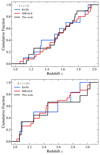 |
Fig. 1. Redshift cumulative distributions of our GRB host sample, compared to the host galaxies of unbiased GRB samples (SHOALS and BAT6). Objects are divided into two bins of redshifts. Top panel with GRB hosts at 1 < z < 2. Bottom panel with GRB hosts at 2 < z < 3.1. |
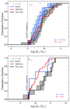 |
Fig. 2. Stellar mass cumulative distributions of our GRB host sample, compared to the host galaxies of unbiased GRB samples (SHOALS and BAT6). Two bins of redshift are distinguished: with GRB hosts at 1 < z < 2 (top panel) and with objects at 2 < z < 3.1 (bottom panel). Upper limits are represented as arrows at the top of the plots. The 1σ uncertainty on the cumulative distribution is given by the shaded region around the curve. The p-value returned by the two-sided K–S test is provided in the right bottom part of both panels and color-coded according to the unbiased sample selected to compute the test. The vertical dashed line symbolizes the stellar mass completeness limit of the 3D-HST survey. |
3. Methods and measurements
3.1. GALFIT modeling of GRB hosts
3.1.1. Profile fitting
We determined the structural parameters of the GRB host galaxies using a parametric approach based on GALFIT (Peng et al. 2002, 2010). GALFIT is a software using a 2D fitting algorithm to model the surface brightness of galaxies. It allows for the fitting of commonly used astronomical brightness profiles including exponential, Sérsic, Nuker, Gaussian, King, Moffat, and PSF. We fit the GRB host galaxies using a unique single Sésic profile to have a similar approach to the 3D-HST sample (van der Wel et al. 2012, 2014). Because we have more than a few galaxies to analyze, we automated the following process in PYTHON. First, we created a cutout of 200 × 200 pixels around the host galaxy position. We then ran SExtractor (Bertin & Arnouts 1996) on the resulting cutout to detect all objects present in the image. We used the segmentation map returned by SExtractor to mask all unnecessary sources. Close, large, or bright sources to the target object are fit simultaneously to reduce their possible contamination. However, fitting many objects increases the number of free parameters and can make GALFIT converge to a local minimum. To choose the neighboring objects to be included in the analysis, we used similar conditions, as described in Vikram et al. (2010). We observe that their conditions based on the isophotal surface and semi-major axis of objects give good results. For the remaining unmasked objects, we modeled them using single Sérsic profile. We initialized the parameters of each component to the values returned by SExtractor through MAG_AUTO, FLUX_RADIUS, ELONGATION, and THETA_IMAGE. We note that the empirical formula, Re = 0.162 × FLUX_RADIUS1.87, determined by Häussler et al. (2007) can help to converge in some cases. Finally, we started the Sérsic index at an exponential profile (n = 1). If GALFIT was not shown to converge, we progressively increased the value.
SExtractor tends to overestimate the sky level (Häussler et al. 2007). For this reason, we set the input sky level at the SExtractor value and let GALFIT optimize simultaneously the sky value and the other components. We also let GALFIT internally determine its own sigma image (noise map). The calculation is described in the GALFIT user’s manual (Eq. (33)). It takes into account the Poisson source noise in addition to the uncertainty on the sky estimation. HLA products are given in electrons/s and have to be converted in electrons before computing the noise map (GALFIT requirement). We multiplied the image by the EXPTIME keyword from the fits header to go back in e− unit. GALFIT considers two additional keywords from the fits header: GAIN (detector gain) and NCOMBINE (number of combined images). As we were already working in electrons unit (not in counts), we set the GAIN keyword to 1. For HLA products, the EXPTIME value already includes the total exposure time from each individual frame. We thus set the NCOMBINE keyword to 1.
GALFIT needs the instrumental response, also known as the point spread function (PSF), to convolve its models and improve the fitting process. To create a PSF model for the HST, three methods are possible: using an empirical model by stacking isolated and bright point-like sources from observations, using a synthetic model from TinyTim modeling software, or using a combination of the two. Models created by TinyTim (Krist et al. 2011) are often not adapted for data analysis due to instrumental effects such as spacecraft jitter or instrument breathing. They need to be corrected for a better matching. Moreover, it is not feasible to derive an empirical PSF model for each GRB host image. Some GRB host fields are very poor in stars (e.g., GRB 060719). The resulting PSF models would have a low signal to noise ratio (S/N) and may introduce artifact in the GALFIT model. To obtain a PSF model with a high S/N, we extracted and combined the stars from all GRB host fields. We isolated a total of 35 stars that we provide to PSFEx (Bertin et al. 2011) to generate a PSF. Then we investigated the possible effects of the PSF modeling. To do so, we applied our wrapper with different PSF models on all GRB hosts at 1 < z < 2. We used two PSFs derived in a rich-stars and poor-stars fields in addition to the one combining stars from all fields. The three PSFs have a similar radius profile but the S/N is progressively degraded as the number of stars used to generate the PSF decreases. We find a good agreement for all parameters, only the Sérsic index varies with the PSF used, as it tends to increase as the S/N of the PSF decreases. Since our study is mainly focused on the half-light radius of GRB host galaxies, we conclude that using the PSF combining stars from multiple fields would not significantly affect our results.
We investigated whether our values determined by GALFIT are consistent with those inferred by van der Wel et al. (2014). Our measurements on the randomly selected objects from the 3D-HST catalog show a good agreement with their estimates (see Appendix B for details). The half-light radii are recovered within 10% at a magnitude of 21.5 (bottom panel of Fig. B.1). We tended to progressively overestimate the Re as the magnitude increases until reaching 50% at a F160W magnitude of 26. Given that our GRB hosts above the 3D-HST mass-completeness limit have magnitudes below 25, we conclude that our fitting procedure is consistent with that of van der Wel et al. (2014) and that the comparison between GRB hosts and 3D-HST objects does not suffer from a strong systematic bias.
3.1.2. Uncertainties
It is widely known that GALFIT tends to underestimate the uncertainties associated with the model parameters (Häussler et al. 2007). To improve the uncertainty estimates for GRB host models, we use a Monte Carlo (MC) approach. First, we consider the best-fitting models returned by GALFIT to create artificial sources. We then inject these sources into randomly selected 50-pixels5 empty regions of the science image. For all objects, the box size is maintained constant to probe environments with similar neighboring objects. We perform one hundred realizations for each object. Finally, the uncertainties are given by the standard deviation between the realizations and the best model. This method mainly captures the uncertainty from the sky estimation. For most of the objects, we find a higher uncertainties than those of GALFIT, especially for the magnitudes and half-light radii. In some cases when the S/N becomes small or the neighbor contamination is dominant, our MC method determines an error lower than the one derived by GALFIT. For this reason, we consider in our analysis the largest uncertainty returned by GALFIT or the MC approach.
3.1.3. Alternative approach
If GALFIT does not converge, we use an alternative procedure to obtain an equivalent GALFIT model. First, we run GALFIT with Re fixed at the SExtractor value. If GALFIT successfully converges to a realistic model (no parameters between ‘*’ and n < 8), we re-run GALFIT with all parameters except Re fixed at the new model values. Using this method, we can estimate for each object (which has not converged with the standard procedure) a GALFIT model and its uncertainties. The models are thus consistent with the standard approach, except that they are constrained by the SExtractor input value. We used this method for two objects of the full sample (see Sect. 3.2).
3.2. GRB hosts properties
3.2.1. Structural parameters
The structural parameters and their uncertainties are presented in Table 1. We provide, for each host galaxy, the F160W AB magnitude, the half-light radius, the Sérsic index, and the axis ratio returned by GALFIT. A total of 35/37 GRB host galaxies converge successfully to realistic parameters. The models and the residuals maps are visible in Figs. C.1.
We used a specific treatment for the host galaxy of GRB 080319C. Perley et al. (2009) and Lyman et al. (2017) reported that a bright foreground galaxy is probably superimposed on the true host galaxy. The redshift of this object was determined from absorption lines in the GRB afterglow. No spectroscopic observations were performed to confirm the association with the host galaxy. The results of GALFIT using a single Sérsic model show a residual source located to the south-east of the main object. This source is consistent with the GRB position and supports the hypothesis that an object is overlapping the true host. We use two Sérsic components to model and mitigate the contamination of the superimposed object. We then add a single Sérsic component to the overall GALFIT model to fit the residual source near the GRB location. The host galaxies of GRB 070802 and GRB 090404 do not converge to realistic parameters (n > 8) with the standard approach. We note that bright sources are close to the host galaxy and likely contaminate it. For these objects, we used the procedure described in Sect. 3.1, where the Re is maintained at the SExtractor value. Finally, the host galaxies of GRB 060502A and 050406X do not converge even when keeping the Re fixed at the first guess of SExtractor. These objects are very faint sources with a low S/N and might diverge numerically easily due to contamination by neighboring objects.
Blanchard et al. (2016), Lyman et al. (2017), and Chrimes et al. (2019) reported the measurement of half-light radii using SExtractor for GRB hosts mainly observed by the WFC3 in the F160W filter. A fraction of our GRB hosts matches their objects. The comparison between their SExtractor and our GALFIT values is shown in Fig. 3. We find good agreement for objects with a Re greater than the full width at half maximum (FWHM) of the PSF. For objects with a half-light radius derived by SExtractor and close to the FWHM, we find that GALFIT returns smaller Re. We expect this behavior because GALFIT convolves its models with the PSF function. It can therefore capture smaller structures of the galaxy.
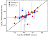 |
Fig. 3. Half-light radius of GRB hosts estimated by GALFIT in this work (x axis) compared to estimates based on SExtractor extracted from the literature (y axis). The FWHM of the PSF is visible as a gray dashed line. |
3.2.2. Stellar mass
The stellar masses of GRB host galaxies used in this work were mostly gathered from the literature. For some objects, we find multiple estimates where most of them were obtained with SED fitting using several photometric points. Only stellar masses from Perley et al. (2016b) were derived using a single photometric point (Spitzer/IRAC 3.6 μm band) and a method based on a mass-redshift grid of galaxy SED models. We compare all these estimates in Fig. 4 (top panel) and we note a significant discrepancy in many cases (up to ∼0.9 dex). The SED fitting codes based on an energy balance principle (e.g., CIGALE, Noll et al. 2009; Boquien et al. 2019) can model the stellar luminosity absorbed by dust and its re-emitted luminosity in the IR. If a far-infrared (FIR) band is used to constrain the models, a more realistic attenuation value can be derived and thus we expect a more accurate stellar mass. For this reason, we selected (preferentially) the estimates in the following order: (1) SED fitting with optical/near-IR (NIR) and FIR measurements using an energy balance code; (2) SED fitting with optical/NIR measurements; and (3) a mass-to-light ratio.
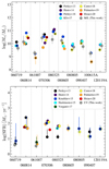 |
Fig. 4. Compilation of stellar mass (top panel) and SFR (bottom panel) estimates for GRB hosts at 1 < z < 2. Each circle corresponds to an estimate from the literature or determined as described in Sect. 3.2. The circles marked with a star represent the estimates used in our analysis. |
For GRB hosts with no stellar mass reported in the literature and not enough photometric points to determine a stellar mass from a SED fitting, we derived our own estimate based on a mass-to-light (M/L) ratio (Bell & de Jong 2001) applied to the F160W magnitude determined by GALFIT. We used the COSMOS2015 (Laigle et al. 2016) catalog to find a relation between stellar mass and NIR luminosity at a given redshift. The COSMOS2015 survey covers a larger area (∼2 degree2) than the 3D-HST/CANDELS survey and gives access to a larger number of galaxies (> 500 000 objects). The catalog provides a total of 16 photometric bands from the ultraviolet to the mid-infrared, including the H band (λmean ∼ 1.64 μm) of the VISTA infrared camera. Given that magnitudes of GRB hosts are obtained with WFC3/F160W filter (λmean ∼ 1.54 μm), we applied a color correction on each GRB host magnitude. To estimate this value, we matched the objects that were observed in the 3D-HST/COSMOS field and the COSMOS2015 catalog. We measured a mean difference of 0.08 mag between the two filters. Finally, we corrected the GRB host galaxy magnitudes for the Galactic extinction using the measurements from Schlafly & Finkbeiner (2011).
To determine the M/L ratio, we first selected all the star-forming galaxies (CLASS=1) from the COSMOS2015 catalog at ztarget ± 0.1. We then fit a linear relation between HVISTA magnitudes and stellar masses of the identified objects. We finally used the linear model and the GRB host magnitudes earlier corrected for color excess and Galactic extinction to obtain the stellar mass. We note that our M/L ratio is based on magnitude in COSMOS2015 determined from aperture photometry using SExtractor, while our magnitude is determined by GALFIT. Skelton et al. (2014) showed that for the 3D-HST catalog the median difference is lower than 0.04 mag in the range 21 < HF160W < 24 between SExtractor and GALFIT measurements. We did not correct for this effect, which would have only a minimal consequence on the estimated stellar mass. In addition, we compared the stellar masses derived using the COSMOS2015 catalog with those calculated from the M/L ratios of the 3D-HST catalog. We find a good agreement between the two estimates for the entire sample of GRB hosts. In our analysis, we used the estimates from the COSMOS2015 catalog, which are based on a larger statistic. The uncertainties are derived by propagating the uncertainty of the GALFIT magnitude models6. We select all galaxies inside ztarget ± 0.1 and with a magtarget ± δmagtarget. We then computed the 1σ error by taking the 16th percentile and 84th percentile of the resulting galaxy distribution.
As a sanity check, we also applied this M/L procedure to the hosts with stellar masses determined in the literature and selected according to the requirements described above. The comparison between the two is visible in Fig. 5, where we color-code the GRB hosts according to their redshift. We find an overall agreement between the two estimates, but we also note a linear trend evolving with stellar mass, where low (high) stellar mass galaxies tend to be overestimated (underestimated). In particular, two GRB hosts have mass estimates differing by more than 0.8 dex (GRB 071021 and GRB 090404). These sources are located at z > 2.4 where the WFC3/F160W filter probes bluer wavelengths, more subject to dust extinction. As GRB host magnitudes are not corrected for galaxy attenuation, they might lead to underestimate the stellar mass derived from a M/L ratio. In addition, we use a single Sérsic profile to model each GRB host galaxy. This enabled us to catch most of the flux for the majority of objects, but in some cases (e.g., GRB 080207, GRB 111215A), more components would have been required to improve the fit and the magnitude estimate. This might have contributed to underestimate their total flux and therefore their stellar mass. With this caution in mind, we note however that the few GRB hosts with mass estimates relying on this M/L approach (see Table 1) have redshifts and stellar masses in the range where Fig. 5 reveals consistent results with the more conventional SED fitting method. This supports therefore the reliability of our measurements, which should not introduce any additional systematics given their otherwise large statistical uncertainties.
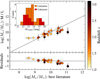 |
Fig. 5. Stellar mass of GRB hosts estimated from mass-to-light ratios, compared with the best estimates selected from the literature (Sect. 3.2). The residuals are shown in the bottom panel. Each GRB host is color-coded according to its redshift. The inset represents their associated F160W magnitude distribution (orange histogram) and the distribution of the GRB hosts for which no stellar mass measurement exists in the literature (red histogram). |
3.2.3. Star formation rate
The star formation rates of GRB host galaxies are also gathered from the literature. In a similar way to stellar masses, we show in Fig. 4 (bottom panel), the dispersion of SFR measurements obtained for a same sources. We yet observe a better agreement between SFRs than previously found for M∗. We note in several cases that the SED fitting solution used to estimate these star formation rates (e.g., Corre et al. 2018; Palmerio et al. 2019) was constrained using SFR measurements determined from emission lines fluxes published in other works (e.g., Krühler et al. 2015). This contributes to reduce the dispersion between estimates observed in Fig. 4. In general, it is expected that estimates including observations in the FIR give a more reliable SFR because the thermal emission of cold dust heated by O/B stars is more accurately modeled. We therefore preferentially select the SFR estimated by (1) SED fitting with optical/NIR and FIR measurements using energy balance code, (2) Dust corrected Hα luminosity (3) SED fitting with optical/NIR measurements. Only for GRB 070306, we consider the SFR based on Hα luminosity instead of the SED fitting with FIR observations. Indeed, the SED of the galaxy in Hsiao et al. (2020) does not match correctly the Herschel/PACS observations. The model seems to underestimate the IR luminosity and thus the total SFR of the galaxy, as also suggested by the higher SFR estimate obtained from Hα. At 1 < z < 2 we have a majority (10/11) of SFRs from Hα and one estimate based on SED fitting including a FIR measurement (ALMA detection). The tracers are more diversified at 2 < z < 3.1 with 5 over 9 objects from SED fitting with ALMA detection, one from Hα, two from SED fitting with optical/NIR measurements and one from the rest-frame UV continuum emission.
If no SFR is found in the literature, we derived a lower limit value based on the R-band magnitude of Hjorth et al. (2012). This filter probes the UV rest-frame of the galaxy at z > 1. The UV light is mainly radiated by young and short-lived stars. It is another indicator of recent SFR in the galaxy. However, the UV radiation is subject to dust reddening caused by the Galactic center or the galaxy itself. We corrected UV magnitudes from the Galactic extinction using Schlafly & Finkbeiner (2011) measurements. We then derived a SFRUV using the relation from Kennicutt (1998). Nevertheless, we only considered these values as lower limits of the SFR since the UV luminosities are not corrected for the dust attenuation in the host itself.
3.3. Stellar mass and star formation surface densities
For GRB hosts and star-forming galaxies, the stellar mass density is given by
where M is the stellar mass in M⊙, and the star formation surface density by
The M∗ and SFR are divided by the galaxy projected area defined by the half-light radius. As it contains half of the total light of the galaxy, a correction factor of 1/2 is applied to the M∗ and SFR while assuming that the matter is uniformly distributed inside the galaxy. We derived the ΣM and ΣSFR errors by propagating the uncertainties of the stellar masses, the star formation rates, and the half-light radii.
3.4. Statistical tests
We applied the Kolmogorov-Smirnov (K–S) test to compare the CDFs of GRB hosts and field galaxies. We considered a similar Bayesian inference framework as described by Palmerio et al. (2019). This approach considers that each parameter value (Re, ΣM, ΣSFR) is described by an asymmetric Gaussian. The center of the distribution is given by the value in Table 1 and the asymmetrical standard deviation is given by errors associated with that value. We sampled each Gaussian probability density function (PDF) with 10 000 (Nreal) MC realizations. We then built Nreal different CDFs for the GRB hosts and 3D-HST samples. Finally, we computed Nreal MC realizations of the two sided K–S test from the previous samples of CDFs. We thus obtained a distribution function of D-statistic and p-values that provide confidence bounds on the K–S test.
4. Results
4.1. Re − M* relation
In Fig. 6 (top panel), we show the half-light radii (Re) against stellar masses for the GRB hosts and 3D-HST star-forming galaxies. As mentioned previously, it is commonly accepted that long GRBs are related to recent star formation activity in their host. If GRB hosts trace the star-forming sources with no bias, then galaxies with higher SFR should have a higher probability of producing a GRB. Based on this assumption, we weighted the control sample by its SFR to mimic a population of galaxies that should host GRBs with no environmental dependence. The resulting SFR-weighted Re − M∗ relation (cyan curve) is close to the median relation characterizing the field galaxies (gray curve). This is expected because for a given stellar mass, the radius does not depend much on the SFR, as can be seen from the sizes of the gray circles in Fig. 6. The 1σ uncertainty associated with the SFR-weighted Re − M∗ relation (cyan region) was derived using the median absolute deviation (MAD) estimator.
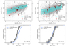 |
Fig. 6. Size-mass relations and size deviations of GRB hosts from star-forming galaxies. Top panels: half-light radius against stellar mass for GRB hosts and star-forming galaxies at 1 < z < 2 (left panel) and 2 < z < 3.1 (right panel). The GRB host galaxies are displayed as red circles and the 3D-HST star-forming galaxies are shown as gray circles with an area proportional to their SFR. The median of the star-forming population is shown as a dashed gray line. The dashed cyan line represents the expected median of a GRB hosts population that does not suffer from bias to trace the SFR (gray circles weighted by their SFR). The 1σ uncertainty of the cyan median is given as a shaded cyan region. The vertical dashed black line is the mass-completeness limit of the 3D-HST survey. Bottom panels: cumulative distribution of Δ(Re − M∗) at 1 < z < 2 (left panel) and 2 < z < 3.1 (right panel). The Δ(Re − M∗) represents the distance between GRB hosts and the SFR-weighted Re − M∗ relation of the top panels. The blue curve is a Gaussian CDF with a mean of 0 and a standard deviation defined by the 1σ errors of the shaded cyan area at the GRB hosts positions. The p-value returned by the two-sided K–S test is provided in the right bottom part of panels. |
Figure 6 (top left panel) clearly shows that GRB hosts are markedly different from the general population. Indeed, we note a larger number of GRB hosts below the SFR-weighted relation at 1 < z < 2. If GRB hosts were truly representative of the overall population of star-forming sources, we would expect approximately equal numbers above and below the SFR-weighted relation. For GRB hosts at 2 < z < 3.1, we observe however a more uniform distribution of sizes with respect to field galaxies, and a better agreement with the SFR-weighted relation. The predominance of dark GRB hosts in the samples and how these results are representative of the whole GRB host population will be further discussed in Sect. 4.3.
Because GRB hosts commonly occur in faint and low stellar mass galaxies (Fruchter et al. 2006) and given the positive trend of the Re − M∗ relation (massive galaxies are also larger), a straight comparison between the distribution of their sizes and that of the overall population of star-forming sources, irrespective of their stellar mass, would necessarily be biased. To quantify if GRB host galaxies are not smaller only because they explode in faint galaxies, we measure for each GRB host the distance between its position in Fig. 6 (top panel) and the SFR-weighted Re − M∗ relation at the same stellar mass, denoted as Δ(Re − M∗) hereafter, such that

If GRB hosts are representative of field star-forming sources, we should expect that the CDF of Δ(Re − M∗) to be distributed around zero. To test this assumption, we applied a K–S test, as described in Sect. 3.4, only considering GRB hosts and field galaxies above the 3D-HST mass-completeness limits quoted earlier. We compared the Δ(Re − M∗) CDF to a Gaussian CDF centered on zero and with a standard deviation given by the median value of the 1σ uncertainties associated with the SFR-weighted relation at each GRB host position. The CDFs and their associated uncertainties are shown in Fig. 6 (bottom panel). For GRB hosts at 1 < z < 2, the two sided K–S test returns a probability of PKS = 0.006. We can rule out the null hypothesis that the two samples are drawn from the same underlying population. At 2 < z < 3.1, we obtain a K–S probability of PKS = 0.47. In this case, the null hypothesis of the K–S test cannot be rejected and we cannot rule out the possibility that both samples are drawn from the same distribution.
4.2. ΣM − M* and ΣSFR-M* relations
Figures 7 and 8 (top panels) show stellar mass and star formation surface densities against stellar mass for GRB hosts and field galaxies. At 1 < z < 2, we note for the ΣM − M∗ and ΣSFR − M∗ planes (top left panels) that the GRB sample is clearly different from the general population, with GRB hosts being placed in a region with higher density values. Regarding the stellar mass densities, we find indeed a larger number of GRB hosts above the SFR-weighted ΣM − M∗ relation at 1 < z < 2, while a more homogeneous distribution of host galaxies is found at 2 < z < 3.1 with respect to the field. This is probably a direct consequence of the trend discussed earlier regarding the size distribution of GRB host galaxies, as the hosts at 1 < z < 2 appear to be smaller (and therefore denser) than typical star-forming sources at comparable stellar masses (see Fig. 6). Similarly, we see that GRB hosts at 1 < z < 2 exhibit star formation surface densities often higher than typically measured in the field, as a larger number of GRB hosts lie above the SFR-weighted ΣM − M∗ relation. At 2 < z < 3.1, our results are nonetheless more intriguing, as we observe an opposite trend where the majority of GRB hosts are below the SFR-weighted ΣSFR − M∗ relation.
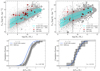 |
Fig. 7. Stellar mass surface density (ΣM) against stellar mass for GRB hosts and star-forming galaxies (top panels) and cumulative distribution of Δ(ΣM − M∗) (bottom panels). The symbols are identical to those of Fig. 6. |
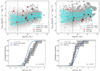 |
Fig. 8. Star formation rate surface density (ΣSFR) against stellar mass for GRB hosts and star-forming galaxies (top panels) and cumulative distribution of Δ(ΣSFR − M∗) (bottom panels). Lower limits are represented as arrows and other symbols are identical to those of Fig. 6. |
In a similar way to the approach we followed to compare the size distribution, we then measured the distance between the GRB hosts and the SFR-weighted ΣM − M∗ relation, denoted as Δ(ΣM − M∗), and expressed as

and the distance between the GRB hosts and the SFR-weighted ΣSFR − M∗ relation, denoted as Δ(ΣSFR − M∗), such that

We then computed their CDFs using the prescriptions given in Sect. 3.4. The CDFs are shown in the bottom panels of Figs. 7 and 8. We compare these CDFs to a CDF centered on zero defined in a similar manner as for the Δ(Re − M∗) parameter. At 1 < z < 2, for both parameters we observe a fraction > 70% of GRB hosts with a distance > 0 to their SFR-weighted relation. We obtain a p-value of PKS = 0.007 and PKS = 0.011 for the Δ(ΣM − M∗) and Δ(ΣSFR − M∗), respectively. We can rule out the null hypothesis in both cases. In other words, the K–S test suggests that the GRB host sample is a distinct population from the general star-forming galaxy population. At 2 < z < 3.1, the median of K–S realizations for Δ(ΣSFR − M∗) rejects the null hypothesis at the 3% significance level but can also be reconciled with the null hypothesis given the K–S uncertainty. Finally at 2 < z < 3.1 for Δ(ΣM − M∗), the K–S test confirms that GRB host galaxies have stellar mass surface densities consistent with those typically found among star-forming sources with similar stellar mass.
4.3. Hosts of GRBs with dark versus optically bright afterglows
We further investigate whether the deviations found may be due to a predominance of dark GRB hosts in the sample and how these results may be extended to the whole GRB host population. Previous studies on the nature of dark bursts and the properties of their host galaxy found a population of galaxies more massive, with a typical stellar mass of about 1010 M⊙, more luminous and with redder colors than optically bright GRB hosts (Krühler et al. 2011; Rossi et al. 2012; Svensson et al. 2012; Perley et al. 2013, 2016b; Hunt et al. 2014). Only a few cases of dark GRBs with low-mass host galaxies have been reported (e.g., GRB 080605 and GRB 100621A, Krühler et al. 2011). The apparent relation between dark GRBs and massive galaxies suggests that the GRB obscuration is mainly due to the dust within the host rather than a dense local environment (clumps) surrounding the GRB. Although a more complex situation with a combination of the two is more likely to be realistic, Corre et al. (2018), for instance, showed that for half of their sample, a very clumpy local dust distribution near the burst is necessary to reproduce the galaxy attenuation curves. Furthermore, Chrimes et al. (2019) analyzed a sample of 21 dark GRBs observed with the HST in F606W and F160W filters. They found that dark GRB host galaxies are physically larger but have a morphology (i.e., spirals or irregulars) similar to those of optically bright GRB hosts. They reported no particular evidence of differences in concentration, asymmetry, or ellipticity between the two populations. These findings support the view that dark and optically bright GRB hosts share common morphological properties, except, not surprisingly, for the galaxy size (galaxies with higher stellar mass are also larger, van der Wel et al. 2014).
At 1 < z < 2 and for 9 ≤ log(M*/M⊙) ≤ 10.2, the two host subpopulations of dark and optically bright GRB afterglows exhibit properties that overlap each other (as seen in the top left panel of Fig. 6). For these sources, we first investigated the distributions of dark versus optically bright GRB hosts in the Re − M∗ plane. To prevent the effect of the positive mass-size trend, we used the Δ(Re − M∗) and calculate a median value for each population. We found a median offset of −0.113, −0.105, and −0.109 dex (i.e., ∼22% smaller) for dark hosts, optically bright hosts, and the whole subsample, respectively. This indicates that at this redshift range, the size distributions of the two population are consistent with each other, and that the tendency for GRB host galaxies to be smaller than the field is not driven by the large number of dark GRBs within our initial selection. In addition, we note that the median Sérsic index and axis ratio are also similar for both populations, which supports that the dark and optically bright GRB hosts share similar morphological properties, at least for this stellar mass range. As suggested by the Re − M∗ plane, we also find that the two populations are consistent in terms of Δ(ΣM − M∗). In the case of Δ(ΣSFR − M∗), the lower statistic makes the comparison more challenging. We note, however, that the two remaining optically bright hosts are in favor of a consistent trend between the two populations.
At 2 < z < 3.1, our sample is mainly composed of dark GRB hosts with log(M*/M⊙) > 10.5. Therefore, it is not possible to extend the comparison between the two subpopulations of host galaxies as discussed above and additional HST observations of the hosts of bright afterglows would be needed to draw a firm conclusion about the properties of the whole GRB host population in this redshift range. Because the radii of dark GRB hosts appear more consistent with the size of field galaxies at 2 < z < 3.1, we argue that a different behavior for the size of the hosts of optically bright GRB afterglows would be difficult to interpret. In this case, indeed, we would have to explain either why the latter remain more compact than the host of dark GRBs despite their lower obscuration or why they become on the other hand much larger than field sources. However, in the absence of clear observational constraints on their physical size, we acknowledge that caution should be considered regarding the interpretation of our results for this redshift range.
4.4. Evolution across z
The results previously described in Sects. 4.1 and 4.2 reveal that a deviation between GRB hosts and field star-forming galaxies on the Re − M∗, ΣM − M∗ and ΣSFR − M∗ planes exists at 1 < z < 2. We further investigate how this deviation compares with the trend previously discussed in the literature for GRB hosts at z < 1.
At 0.3 < z < 1.1, we use a GRB host sample extracted jointly from Kelly et al. (2014) and Blanchard et al. (2016). Their respective selections are not drawn from unbiased GRB samples. We use a similar method to the one described in Sect. 2.4 and evaluate how the CDFs in redshift and stellar mass are distributed compared to the hosts of unbiased GRB samples (BAT6 and SHOALS). The results are presented in Fig. 9. We find that the CDFs are consistent with each other for both parameters. This confirms that our sample at 0.3 < z < 1.1 probes a similar range of stellar masses as the host galaxies of unbiased GRB samples and that our sample does not suffer from an important bias toward low- or high-mass galaxies.
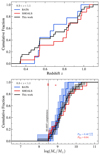 |
Fig. 9. Cumulative distributions as in Fig. 1 (top panel) and Fig. 2 (bottom panel) but showing the GRB host sample combined from Kelly et al. (2014) and Blanchard et al. (2016) at 0.3 < z < 1.1. |
In addition, to enable a comparison as fair as possible with our previous work at z > 1 and limit the potential systematic bias between the different studies, we only considered the size measurements reported by these authors. We then recomputed the ΣM and ΣSFR using M∗ and SFR extracted from literature in a way similar to the one described in Sect. 3.1. From Kelly et al. (2014), we selected the r50 determined from the SDSS photo pipeline. A part of their sample matches the sample of Wainwright et al. (2007) who used GALFIT and a single Sérsic profile to measure galaxy sizes. The comparison of estimates shows good agreement between the two methods. This confirms that using sizes from the SDSS photo pipeline should not introduce a significant bias compared to our method. From Blanchard et al. (2016), we select Re determined by SExtractor. In Fig. 3, we show that the majority of size measurements are consistent between GALFIT and SExtractor, except when the galaxy size becomes close to the PSF size. Given that only 2/18 objects at z < 1 are smaller than the PSF size, this effect should not significantly affect the results. Finally, the majority of the objects (13/18) were observed with the F160W filter of the WFC3/IR camera. The others were targeted with a filter close to the R-band, which also mostly probes the bulk of the stellar component for these sources at low redshift. Hence, it should not introduce any additional bias to our study.
In Kelly et al. (2014), GRB hosts are compared to a sample of star-forming galaxies from the Sloan Digital Sky Survey (SDSS) DR10 catalog at z < 0.2. Because a non-negligible fraction of our combined GRB host low-redshift sample is located at z > 0.2, we were able to perform a new comparison by considering a control sample from the 3D-HST survey at similar redshift, applying the same analysis method as performed at 1 < z < 2 and 2 < z < 3.1. Although 3D-HST may be more suited to galaxies at larger distances (i.e., z > 1), we note that this survey remains the most appropriate when combining estimates of redshift, size, stellar mass, and star formation rates for sources at low to intermediate redshifts. It represents therefore the best available control sample to study the densities of GRB hosts at 0.3 < z < 1.1. Our combined sample of GRB host galaxies at 0.3 < z < 1.1 yields similar results to those obtained by Kelly et al. (2014). We indeed found that the majority of GRB hosts are located above the SFR-weighted ΣM − M∗ and ΣSFR − M∗ relations of field galaxies, while they fall below the Re − M∗ relation driven by the control sample of star-forming sources. However, the apparent deviations that we measure are much less pronounced than those derived by Kelly et al. (2014), which may be due to the different control sample used in their analysis. We computed the CDFs for each parameter and perform K–S tests. The results reveal that we can reject the null hypothesis with a significance level of ≲5% for all parameters (PKS = 0.01, PKS = 0.04 and PKS = 0.006 for Δ(Re − M∗), Δ(ΣM − M∗) and Δ(ΣM − M∗), respectively).
In Fig. 10, we show the evolution of Δ(Re − M∗) at 0.3 < z < 3.1. We divided the redshift range in five bins and determine the corresponding median value for each redshift bin. At z ≲ 2, we observe that the median Δ(Re − M∗) is systematically negative, with an offset that appears statistically significant despite the relatively large scatter of the individual estimates. This shows again that the overall population of GRB host galaxies at z ≲ 2 tend to exhibit smaller sizes than typical star-forming sources with comparable stellar masses. As already noticed in Sect. 4.1 from our sample at 2 < z < 3.1, the median value at z ≳ 2 is, however, closer to a null deviation, meaning that GRB hosts at higher redshifts tend to be more homogeneously spread around the SFR-weighted Re − M∗ relation. Similarly, we find an opposite behavior for Δ(ΣM − M∗) (Fig. 11), which reveals a statistically significant positive deviation up to z ∼ 2, and a median value consistent with zero at higher redshift. Finally, the Δ(ΣSFR − M∗) is shown in Fig. 12. We reduce the number of redshift bins due to the smaller number of GRB hosts with a SFR value. We find that GRB host galaxies may show a slight preference toward high star formation density at low to intermediate redshifts, but all median values are also consistent with a null deviation given the large associated uncertainties.
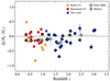 |
Fig. 10. Δ(Re − M∗) as a function of the redshift for GRB host galaxies. The orange and red circles are GRB hosts at z ≲ 1 from Kelly et al. (2014) and Blanchard et al. (2016), respectively. The blue circles are the GRB hosts considered in this study. Dark GRBs are highlighted by a thick black circle. The gray squares are the median of the Δ(Re − M∗) for each redshift bin. The associated error bars are the standard deviation using the MAD estimator. The black line at y = 0 represents the expected median values for a GRB hosts population that do not suffer from environment bias. |
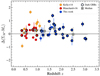 |
Fig. 11. Δ(ΣM − M∗) against redshift for GRB host galaxies. The symbols are identical to those of Fig. 10. |
5. Discussion
The non-negligible scatter observed in Figs. 10–12 unfortunately prevents us from deriving an unambiguous interpretation of the data. However, our analysis strongly suggests that GRB host galaxies up to z ∼ 2 tend to exhibit smaller sizes and larger densities of stellar mass and star formation than what we could expect for a SFR-weighted population of star-forming galaxies. It thus confirms and extends to higher redshifts the trend already observed for GRB hosts at low z, even though the offset that we find between the two populations is not as prominent as previously measured (e.g., Kelly et al. 2014). We stress again that our comparison was performed by properly matching the GRB host sample and the population of field sources in redshift and stellar mass. This indicates that our results cannot be explained by the combination of the more frequent occurrence of long GRBs in low-mass sources (at least up to z ∼ 2) with the general mass-size relationship and its evolution with cosmic time. Similarly, we showed that it cannot be due to systematic uncertainties in the determination of physical parameters (e.g., mass, size) between field galaxies and GRB hosts. Finally, we believe that this effect cannot be simply due to the GRB host sample selection and in particular the larger number of GRBs with a dark afterglow compared to the overall population of long GRBs. A higher number of dark GRBs may indeed bias the host sample toward larger and more massive sources (Perley et al. 2013; Chrimes et al. 2020), but this should not affect the comparison with field galaxies at fixed stellar mass. In addition, we do not observe any apparent difference between dark and optically bright GRB hosts at 1 < z < 2, when quantifying their size, stellar mass, and SFR density offset with the field (Figs. 6–8). This is also what we find with the sample at 0.3 < z < 1.1, which is composed of a majority of optically bright GRBs and that shows a similar trend toward compact and dense environments.
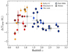 |
Fig. 12. Δ(ΣSFR − M∗) against redshift for GRB host galaxies. Lower limits are represented as arrows and other symbols are identical to those of Fig. 10. |
5.1. Effects of the size-metallicity relation on GRB hosts
Previous works have pointed to the conclusion that the production efficiency of long GRBs is mostly ruled by metallicity, with GRB formation being switched off in galaxies with metallicity higher than a threshold that is still currently debated in the literature (Modjaz et al. 2008; Graham & Fruchter 2013; Krühler et al. 2015; Vergani et al. 2015; Perley et al. 2016b; Palmerio et al. 2019). Given the additional bias toward compact galaxies found in our analysis for GRB hosts, we further investigate the possible link between the size and metallicity of galaxies. Ellison et al. (2008a) used a sample of star-forming sources from the SDSS to study the possible influence of the galaxy size on the mass-metallicity (MZ) relation (Tremonti et al. 2004; Mannucci et al. 2010; Wuyts et al. 2014; Zahid et al. 2014). They observed an anti-correlation between size and metallicity at a given stellar mass. This means that for the same stellar mass, galaxies with a smaller size are also richer in metallicity, (i.e., the metallicity increases by 0.1 dex when the size is divided by a factor of 2). This result has been corroborated by Brisbin & Harwit (2012), Harwit & Brisbin (2015) and it was also observed at higher redshifts by Yabe et al. (2012, 2014) using a sample of star-forming galaxies up to z ∼ 1.4. The tendency for GRB hosts to occur in denser environments could thus appear intriguing at first sight. In fact, GRB-selected galaxies appear to track the mass–metallicity relation of star-forming sources but with an offset of 0.15 dex toward lower metallicities (Arabsalmani et al. 2018). If this offset is due to the intrinsic nature of GRB hosts and not to systematic effects, the possibility that GRB hosts are more compact (and not larger) than field galaxies may indicate that the physical conditions and the environments in which long GRBs form are more complex than what has been assumed so far. Our results could also imply that the impact of metallicity and compactness separately considered is even stronger than has actually been seen, and their inter-correlation at a given stellar mass mitigates the global trends that we can observe among GRB hosts. Interestingly, based on the EAGLE cosmological numerical simulations, Sánchez Almeida & Dalla Vecchia (2018) found a similar size-metallicity anti-correlation up to z ∼ 8 and explored its possible physical origin. It is worth noting that their simulation reproduced well-known observed scale relations such as the MZ relation at z < 5 (De Rossi et al. 2017) but was not designed to reproduce the relation between size and metallicity. They explored three potential explanations of this relation: (1) a recent metal-poor gas inflows that increased the size and reduced the metallicity of the galaxy; (2) a more efficient star formation process in compact galaxies, whereby the denser gas transforming more efficiently into stars, resulting in a faster enrichment of the gas; and (3) an effectiveness of metal-rich gas outflows reduced in compact galaxies due to a deeper gravitational potential. The EAGLE simulation supports cause (1) and discards causes (2) and (3). In this scenario, we may infer that long GRBs cannot be linked to young star formation triggered by recent inflow of gas at low metallicity, which would have otherwise increased the size of their hosting environment.
To investigate this possible relationship between metallicity and stellar density in greater detail in our GRB host sample, we turned to previous studies (Hashimoto et al. 2015; Krühler et al. 2015) to extract the gas-phase metallicity measurement determined from strong emission lines (Zemiss). We only consider GRB hosts in 1 < z < 2, where the trend toward compact galaxies is more clearly observed. We find only a small fraction of GRB hosts (10/22) with a metallicity measurement. We also find an additional GRB host with gas-phase metallicity measurement determined using the GRB afterglow absorption lines (Zabs) in Arabsalmani et al. (2018). However, due to the insecure relation between Zemiss and Zabs especially at high-z (Metha & Trenti 2020; Metha et al. 2021), we omit this measurement. Unfortunately, our data do not reveal any obvious trend between the metallicity of GRB hosts and the deviation of their size from field galaxies at comparable stellar mass. This may be explained by the poor statistics of the sample and, therefore, we cannot confirm or rule out a different relation for GRB hosts compared to field galaxies regarding these physical parameters.
To further complicate the picture, we finally point out that minor interactions could also play a role in shaping the inter-dependency of size and metallicity in these different populations. Using a local sample of star-forming galaxies from the SDSS, Ellison et al. (2008b) observed that galaxies with a companion have indeed a lower metallicity for a given stellar mass and size. Detailed studies of individual GRB host revealed that GRBs can be found in interacting environments (Thöne et al. 2011; Arabsalmani et al. 2019). It is also supported by previous work (Wainwright et al. 2007; Ørum et al. 2020) reporting that GRB hosts are often found in interacting systems with major companions (∼30%). This may suggest that a recent interaction of the host galaxy could also affect the conditions required to produce a long GRB, in addition to metallicity and stellar density.
5.2. A possible redshift-dependent bias
At z ≳ 2, the picture arising from our sample is different than the one observed at lower redshifts. The apparent deviation that we found at z ≲ 2 between GRB hosts and field galaxies seems to disappear. Admittedly, the large uncertainties measured at 2 < z < 3.1 and the much lower statistics characterizing our GRB host sample at such redshifts do not allow us to draw a firm conclusion that this evolution is real and statistically robust, as suggested by the significance of our K–S tests as well. The SFR density of GRB hosts at 2 < z < 3.1 may even be lower than expected from the field according to our analysis (see Fig. 8), although we believe this reversal is probably due to the small number of sources in our sample. However, the data do suggest that the size and stellar mass density of GRB hosts at these higher redshifts are globally more representative of the overall population of star-forming galaxies in the field. From a qualitative point of view, we could argue that this evolution of the size and density of GRB hosts compared to the field is consistent with the idea that the bias, which is clearly established between the overall population of star-forming galaxies and the hosts of long GRBs at low redshifts, which is progressively reduced as the redshift increases. This may thus support the hypothesis that long GRBs represent a more accurate tracer of star formation in the distant Universe than they actually do at lower redshifts. On the other hand, we note that the stellar mass range probed by our sample in this redshift range (M* > 1010.5) is substantially larger than the one probed at 1 < z < 2 (M* < 1010.5), and our GRB host selection at z ≳ 2 is also exclusively drawn from dark GRBs. While we found no apparent difference in the size and stellar densities between the hosts of optically bright and dark GRBs at lower stellar mass and redshift, we cannot firmly exclude a possible dependence of the size deviation with stellar mass. This means that the offset observed at z ≲ 2 could plausibly remain at 2 < z < 3.1, if we had also included GRB hosts with lower stellar mass (M* < 1010.5) or more massive hosts selected with optically bright GRBs.
5.3. Stellar density and GRB progenitor models
Considering the proposed progenitor models, GRB production may be expected to depend on the density environment in addition to any metallicity bias. Several observational and theoretical studies reported that the fraction of star formation happening in young bound star clusters (Γ) may depend on the environmental properties of the host galaxy. In particular, they found that the ΣSFR correlates with Γ (Goddard et al. 2010; Adamo et al. 2011, 2015; Kruijssen 2012; Silva-Villa et al. 2013). Owing to a greater amount of stars, these clusters may more frequently produce binary systems of massive stars which are one of the candidates to form GRBs. However, this has to be set against the results of Chandar et al. (2017; see also Chandar et al. 2015; Kruijssen & Bastian 2016), which showed that the relation between ΣSFR and Γ presents no particular trend. The previously reported correlation would be due to a bias in the selection of galaxies leading to an estimation of Γ mixing young and old clusters. As a consequence, young (old) clusters were systematically associated with high (low) ΣSFR creating an apparent correlation between Γ and ΣSFR. On the other hand, several studies suggest that the IMF can evolve to top-heavy (overabundance of high mass stars) when the density of the environment increases (Marks et al. 2012; Haghi et al. 2020). If the number of massive stars increases, the probability to produce a GRB also increases. This provides a plausible explanation for the reported trend that associates GRBs with compact and dense environments.
6. Summary and conclusions
In this work, we study a sample of long GRB host galaxies observed with the HST/WFC3 in the IR band at 1 < z < 3.1. We compared their sizes, stellar masses, and star formation rate surface densities to the measurements of typical star-forming galaxies of the 3D-HST survey. Prior to the comparison, we minimized the systematics and biases that measurement methods may introduce between samples observed under different conditions. We also verified that no systematic offset is present between the GRB hosts and the star-forming galaxies in the determination of their physical properties. In addition, we confronted our GRB host sample to the host galaxies of unbiased GRB samples (BAT6 and SHOALS). At 1 < z < 2, we found that they are consistent with each other in terms of stellar mass and redshift distributions while at 2 < z < 3.1 we noted an offset toward more massive galaxies. We performed a fair comparison between the GRB hosts and the field galaxies by fixing their redshift range and stellar mass to remove any dependency that the measured properties may have on these two parameters. At 1 < z < 2, the results clearly showed that GRB hosts are smaller in size and have higher stellar mass and star formation rate surface densities than expected if they had truly been representative of the overall population of star-forming galaxies. We also noted that the galaxy size and stellar density are consistent for the dark and optically bright GRB host populations. At 2 < z < 3.1, the trend appears to evolve and GRB hosts seem to be more consistent with star-forming galaxies of the field. We even found an inversion of the tendency for the ΣSFR parameter, where GRB hosts have a lower star formation rate surface density than field sources. However, because of the small sample size at this redshift, we cannot rule out the possibility of a purely statistical effect. Furthermore, we cannot exclude a possible bias in our results at z ≳ 2 due to the predominance of galaxies selected from dark GRBs. We inserted our results into a broader context and considered at 0.3 < z < 1.1 the size measurements from Kelly et al. (2014) and Blanchard et al. (2016). We performed a similar analysis to the one at 1 < z < 3.1 and found that up to z ∼ 2, GRB hosts have a smaller size and a higher stellar mass and star formation surface densities than field galaxies. Finally, we investigated the possible relation between the size and metallicity bias found in the GRB host population. However, due to the limited number of metallicity measurements available in the literature for the GRB hosts in our sample, we cannot confirm or refute the anti-correlation reported for star-forming galaxies in the literature between size and metallicity at a given stellar mass.
These results are part of the effort to better understand long GRB formation and the ability to trace the CSFRH, especially at high-redshift where the trend is still poorly constrained by observations. Future works will be focused on expanding the GRB host sample to confirm the trend observed at z < 3 and extend the analysis at higher redshifts. The forthcoming SVOM mission (Wei et al. 2016; Atteia et al. 2022) and its dedicated follow-up network will allow us to rapidly identify high-z bursts candidate and will contribute to a better controlled and homogeneous GRB host sample. Its synergy with the upcoming James Webb Space Telescope (Gardner et al. 2006) offers a promising opportunity to detect and characterize GRB host galaxies at very high redshift.
More particularly, we use the largest uncertainty values returned by GALFIT or the MC approach, as described in the Sect. 3.1.2.
Acknowledgments
We thank the anonymous referee for insightful comments and a careful reading of the manuscript. We acknowledge the support of the UnivEarths LabEx program and S. D. V. and J. T. P. additionally acknowledge the support of CNES. We also thank A. van der Wel for providing access to the PSF model of 3D-HST/CANDELS mosaics and C. Peng and B. Haüssler for useful discussions about GALFIT. The observations are based on observations made with the NASA/ESA Hubble Space Telescope, and obtained from the Hubble Legacy Archive, which is a collaboration between the Space Telescope Science Institute (STScI/NASA), the Space Telescope European Coordinating Facility (ST-ECF/ESA) and the Canadian Astronomy Data Centre (CADC/NRC/CSA). This work is based on observations taken by the CANDELS Multi-Cycle Treasury Program and the 3D-HST Treasury Program (GO 12177 and 12328) with the NASA/ESA HST, which is operated by the Association of Universities for Research in Astronomy, Inc., under NASA contract NAS5-26555. This research made use of Astropy (https://www.astropy.org), a community-developed core Python package for Astronomy (Astropy Collaboration 2013, 2018), of matplotlib, a Python library for publication quality graphics (Hunter 2007), of Astroquery (Ginsburg et al. 2019) and of NumPy (Harris et al. 2020).
References
- Adamo, A., Östlin, G., & Zackrisson, E. 2011, MNRAS, 417, 1904 [NASA ADS] [CrossRef] [Google Scholar]
- Adamo, A., Kruijssen, J. M. D., Bastian, N., Silva-Villa, E., & Ryon, J. 2015, MNRAS, 452, 246 [NASA ADS] [CrossRef] [Google Scholar]
- Aggarwal, K., Budavári, T., Deller, A. T., et al. 2021, ApJ, 911, 95 [NASA ADS] [CrossRef] [Google Scholar]
- Arabsalmani, M., Roychowdhury, S., Zwaan, M. A., Kanekar, N., & Michałowski, M. J. 2015, MNRAS, 454, L51 [NASA ADS] [CrossRef] [Google Scholar]
- Arabsalmani, M., Møller, P., Perley, D. A., et al. 2018, MNRAS, 473, 3312 [NASA ADS] [CrossRef] [Google Scholar]
- Arabsalmani, M., Roychowdhury, S., Starkenburg, T. K., et al. 2019, MNRAS, 485, 5411 [NASA ADS] [CrossRef] [Google Scholar]
- Arabsalmani, M., Renaud, F., Roychowdhury, S., et al. 2020, ApJ, 899, 165 [NASA ADS] [CrossRef] [Google Scholar]
- Astropy Collaboration (Robitaille, T. P., et al.) 2013, A&A, 558, A33 [NASA ADS] [CrossRef] [EDP Sciences] [Google Scholar]
- Astropy Collaboration (Price-Whelan, A. M., et al.) 2018, AJ, 156, 123 [Google Scholar]
- Atteia, J. L., Cordier, B., & Wei, J. 2022, Int. J. Mod. Phys. D, 31, 2230008a [NASA ADS] [CrossRef] [Google Scholar]
- Barden, M., Häußler, B., Peng, C. Y., McIntosh, D. H., & Guo, Y. 2012, MNRAS, 422, 449 [CrossRef] [Google Scholar]
- Bell, E. F., & de Jong, R. S. 2001, ApJ, 550, 212 [Google Scholar]
- Bertin, E. 2011, in Astronomical Data Analysis Software and Systems XX, eds. I. N. Evans, A. Accomazzi, D. J. Mink, & A. H. Rots, ASP Conf. Ser., 442, 435 [Google Scholar]
- Bertin, E., & Arnouts, S. 1996, A&AS, 117, 393 [NASA ADS] [CrossRef] [EDP Sciences] [Google Scholar]
- Blanchard, P. K., Berger, E., & Fong, W.-F. 2016, ApJ, 817, 144 [Google Scholar]
- Bloom, J. S., Kulkarni, S. R., & Djorgovski, S. G. 2002, AJ, 123, 1111 [NASA ADS] [CrossRef] [Google Scholar]
- Boquien, M., Burgarella, D., Roehlly, Y., et al. 2019, A&A, 622, A103 [NASA ADS] [CrossRef] [EDP Sciences] [Google Scholar]
- Brammer, G. B., van Dokkum, P. G., Franx, M., et al. 2012, ApJS, 200, 13 [Google Scholar]
- Brisbin, D., & Harwit, M. 2012, ApJ, 750, 142 [NASA ADS] [CrossRef] [Google Scholar]
- Cantiello, M., Yoon, S. C., Langer, N., & Livio, M. 2007, A&A, 465, L29 [NASA ADS] [CrossRef] [EDP Sciences] [Google Scholar]
- Carnall, A. C., Leja, J., Johnson, B. D., et al. 2019, ApJ, 873, 44 [Google Scholar]
- Chabrier, G. 2003, PASP, 115, 763 [Google Scholar]
- Chandar, R., Fall, S. M., & Whitmore, B. C. 2015, ApJ, 810, 1 [NASA ADS] [CrossRef] [Google Scholar]
- Chandar, R., Fall, S. M., Whitmore, B. C., & Mulia, A. J. 2017, ApJ, 849, 128 [NASA ADS] [CrossRef] [Google Scholar]
- Chrimes, A. A., Stanway, E. R., Levan, A. J., et al. 2018, MNRAS, 478, 2 [NASA ADS] [CrossRef] [Google Scholar]
- Chrimes, A. A., Levan, A. J., Stanway, E. R., et al. 2019, MNRAS, 486, 3105 [NASA ADS] [CrossRef] [Google Scholar]
- Chrimes, A. A., Stanway, E. R., & Eldridge, J. J. 2020, MNRAS, 491, 3479 [NASA ADS] [CrossRef] [Google Scholar]
- Conselice, C. J., Vreeswijk, P. M., Fruchter, A. S., et al. 2005, ApJ, 633, 29 [NASA ADS] [CrossRef] [Google Scholar]
- Corre, D., Buat, V., Basa, S., et al. 2018, A&A, 617, A141 [NASA ADS] [CrossRef] [EDP Sciences] [Google Scholar]
- De Rossi, M. E., Bower, R. G., Font, A. S., Schaye, J., & Theuns, T. 2017, MNRAS, 472, 3354 [Google Scholar]
- Ellison, S. L., Patton, D. R., Simard, L., & McConnachie, A. W. 2008a, ApJ, 672, L107 [NASA ADS] [CrossRef] [Google Scholar]
- Ellison, S. L., Patton, D. R., Simard, L., & McConnachie, A. W. 2008b, AJ, 135, 1877 [NASA ADS] [CrossRef] [Google Scholar]
- Förster Schreiber, N. M., & Wuyts, S. 2020, ARA&A, 58, 661 [Google Scholar]
- Fruchter, A. S., Levan, A. J., Strolger, L., et al. 2006, Nature, 441, 463 [NASA ADS] [CrossRef] [Google Scholar]
- Fryer, C. L., & Heger, A. 2005, ApJ, 623, 302 [Google Scholar]
- Fynbo, J. P. U., Jakobsson, P., Prochaska, J. X., et al. 2009, ApJS, 185, 526 [NASA ADS] [CrossRef] [Google Scholar]
- Gardner, J. P., Mather, J. C., Clampin, M., et al. 2006, Space Sci. Rev., 123, 485 [Google Scholar]
- Ghirlanda, G., & Salvaterra, R. 2022, ApJ, 932, 10 [NASA ADS] [CrossRef] [Google Scholar]
- Ginsburg, A., Sipőcz, B. M., Brasseur, C. E., et al. 2019, AJ, 157, 98 [Google Scholar]
- Goddard, Q. E., Bastian, N., & Kennicutt, R. C. 2010, MNRAS, 405, 857 [NASA ADS] [Google Scholar]
- Graham, J. F., & Fruchter, A. S. 2013, ApJ, 774, 119 [CrossRef] [Google Scholar]
- Greiner, J., Krühler, T., Klose, S., et al. 2011, A&A, 526, A30 [NASA ADS] [CrossRef] [EDP Sciences] [Google Scholar]
- Greiner, J., Fox, D. B., Schady, P., et al. 2015, ApJ, 809, 76 [NASA ADS] [CrossRef] [Google Scholar]
- Grogin, N. A., Kocevski, D. D., Faber, S. M., et al. 2011, ApJS, 197, 35 [NASA ADS] [CrossRef] [Google Scholar]
- Haghi, H., Safaei, G., Zonoozi, A. H., & Kroupa, P. 2020, ApJ, 904, 43 [NASA ADS] [CrossRef] [Google Scholar]
- Harris, C. R., Millman, K. J., van der Walt, S. J., et al. 2020, Nature, 585, 357 [NASA ADS] [CrossRef] [Google Scholar]
- Harwit, M., & Brisbin, D. 2015, ApJ, 800, 91 [NASA ADS] [CrossRef] [Google Scholar]
- Hashimoto, T., Perley, D. A., Ohta, K., et al. 2015, ApJ, 806, 250 [NASA ADS] [CrossRef] [Google Scholar]
- Hashimoto, T., Hatsukade, B., Goto, T., et al. 2019, MNRAS, 488, 5029 [NASA ADS] [CrossRef] [Google Scholar]
- Häussler, B., McIntosh, D. H., Barden, M., et al. 2007, ApJS, 172, 615 [Google Scholar]
- Heintz, K. E., Malesani, D., Wiersema, K., et al. 2018, MNRAS, 474, 2738 [NASA ADS] [CrossRef] [Google Scholar]
- Hjorth, J., Sollerman, J., Møller, P., et al. 2003, Nature, 423, 847 [Google Scholar]
- Hjorth, J., Malesani, D., Jakobsson, P., et al. 2012, ApJ, 756, 187 [Google Scholar]
- Hsiao, T. Y.-Y., Hashimoto, T., Chang, J.-Y., et al. 2020, MNRAS, 496, 4405 [NASA ADS] [CrossRef] [Google Scholar]
- Hunt, L. K., Palazzi, E., Michałowski, M. J., et al. 2014, A&A, 565, A112 [NASA ADS] [CrossRef] [EDP Sciences] [Google Scholar]
- Hunter, J. D. 2007, Comput. Sci. Eng., 9, 90 [NASA ADS] [CrossRef] [Google Scholar]
- Jakobsson, P., Hjorth, J., Fynbo, J. P. U., et al. 2004, ApJ, 617, L21 [NASA ADS] [CrossRef] [Google Scholar]
- Kangas, T., Fruchter, A. S., Cenko, S. B., et al. 2020, ApJ, 894, 43 [CrossRef] [Google Scholar]
- Kelly, P. L., Filippenko, A. V., Modjaz, M., & Kocevski, D. 2014, ApJ, 789, 23 [NASA ADS] [CrossRef] [Google Scholar]
- Kennicutt, R. C. Jr. 1998, ARA&A, 36, 189 [NASA ADS] [CrossRef] [Google Scholar]
- Kistler, M. D., Yüksel, H., Beacom, J. F., & Stanek, K. Z. 2008, ApJ, 673, L119 [Google Scholar]
- Koekemoer, A. M., Faber, S. M., Ferguson, H. C., et al. 2011, ApJS, 197, 36 [NASA ADS] [CrossRef] [Google Scholar]
- Kriek, M., van Dokkum, P. G., Labbé, I., et al. 2009, ApJ, 700, 221 [Google Scholar]
- Krist, J. E., Hook, R. N., & Stoehr, F. 2011, in Optical Modeling and Performance Predictions V, ed. M. A. Kahan, SPIE Conf. Ser., 8127, 81270J [Google Scholar]
- Krühler, T., & Schady, P. 2017, Photometry and Stellar Masses for GRB Host Galaxies with Emission-line Spectra [Google Scholar]
- Krühler, T., Greiner, J., Schady, P., et al. 2011, A&A, 534, A108 [CrossRef] [EDP Sciences] [Google Scholar]
- Krühler, T., Malesani, D., Fynbo, J. P. U., et al. 2015, A&A, 581, A125 [Google Scholar]
- Krühler, T., Kuncarayakti, H., Schady, P., et al. 2017, A&A, 602, A85 [NASA ADS] [CrossRef] [EDP Sciences] [Google Scholar]
- Kruijssen, J. M. D. 2012, MNRAS, 426, 3008 [Google Scholar]
- Kruijssen, J. M. D., & Bastian, N. 2016, MNRAS, 457, L24 [NASA ADS] [CrossRef] [Google Scholar]
- Laigle, C., McCracken, H. J., Ilbert, O., et al. 2016, ApJS, 224, 24 [Google Scholar]
- Le Floc’h, E., Duc, P. A., Mirabel, I. F., et al. 2003, A&A, 400, 499 [CrossRef] [EDP Sciences] [Google Scholar]
- Levesque, E. M., Kewley, L. J., Graham, J. F., & Fruchter, A. S. 2010a, ApJ, 712, L26 [NASA ADS] [CrossRef] [Google Scholar]
- Levesque, E. M., Bloom, J. S., Butler, N. R., et al. 2010b, MNRAS, 401, 963 [NASA ADS] [CrossRef] [Google Scholar]
- Levesque, E. M., Berger, E., Soderberg, A. M., & Chornock, R. 2011, ApJ, 739, 23 [NASA ADS] [CrossRef] [Google Scholar]
- Lyman, J. D., Levan, A. J., Tanvir, N. R., et al. 2017, MNRAS, 467, 1795 [NASA ADS] [Google Scholar]
- Madau, P., & Dickinson, M. 2014, ARA&A, 52, 415 [Google Scholar]
- Mannucci, F., Cresci, G., Maiolino, R., Marconi, A., & Gnerucci, A. 2010, MNRAS, 408, 2115 [NASA ADS] [CrossRef] [Google Scholar]
- Marks, M., Kroupa, P., Dabringhausen, J., & Pawlowski, M. S. 2012, MNRAS, 422, 2246 [NASA ADS] [CrossRef] [Google Scholar]
- Metha, B., & Trenti, M. 2020, MNRAS, 495, 266 [NASA ADS] [CrossRef] [Google Scholar]
- Metha, B., Cameron, A. J., & Trenti, M. 2021, MNRAS, 504, 5992 [NASA ADS] [CrossRef] [Google Scholar]
- Meurer, G. R., Heckman, T. M., & Calzetti, D. 1999, ApJ, 521, 64 [Google Scholar]
- Michałowski, M. J., Castro Cerón, J. M., Wardlow, J. L., et al. 2016, A&A, 595, A72 [NASA ADS] [CrossRef] [EDP Sciences] [Google Scholar]
- Mobasher, B., Dahlen, T., Ferguson, H. C., et al. 2015, ApJ, 808, 101 [NASA ADS] [CrossRef] [Google Scholar]
- Modjaz, M., Kewley, L., Kirshner, R. P., et al. 2008, AJ, 135, 1136 [NASA ADS] [CrossRef] [Google Scholar]
- Momcheva, I. G., Brammer, G. B., van Dokkum, P. G., et al. 2016, ApJS, 225, 27 [Google Scholar]
- Noll, S., Burgarella, D., Giovannoli, E., et al. 2009, A&A, 507, 1793 [NASA ADS] [CrossRef] [EDP Sciences] [Google Scholar]
- Ørum, S. V., Ivens, D. L., Strandberg, P., et al. 2020, A&A, 643, A47 [NASA ADS] [CrossRef] [EDP Sciences] [Google Scholar]
- Pacifici, C., da Cunha, E., Charlot, S., et al. 2015, MNRAS, 447, 786 [NASA ADS] [CrossRef] [Google Scholar]
- Palmerio, J. T., Vergani, S. D., Salvaterra, R., et al. 2019, A&A, 623, A26 [NASA ADS] [CrossRef] [EDP Sciences] [Google Scholar]
- Peng, C. Y., Ho, L. C., Impey, C. D., & Rix, H.-W. 2002, AJ, 124, 266 [Google Scholar]
- Peng, C. Y., Ho, L. C., Impey, C. D., & Rix, H.-W. 2010, AJ, 139, 2097 [Google Scholar]
- Perley, D. A., & Perley, R. A. 2013, ApJ, 778, 172 [NASA ADS] [CrossRef] [Google Scholar]
- Perley, D. A., Cenko, S. B., Bloom, J. S., et al. 2009, AJ, 138, 1690 [NASA ADS] [CrossRef] [Google Scholar]
- Perley, D. A., Levan, A. J., Tanvir, N. R., et al. 2013, ApJ, 778, 128 [Google Scholar]
- Perley, D. A., Perley, R. A., Hjorth, J., et al. 2015, ApJ, 801, 102 [NASA ADS] [CrossRef] [Google Scholar]
- Perley, D. A., Tanvir, N. R., Hjorth, J., et al. 2016a, ApJ, 817, 8 [Google Scholar]
- Perley, D. A., Krühler, T., Schulze, S., et al. 2016b, ApJ, 817, 7 [Google Scholar]
- Petrovic, J., Langer, N., & van der Hucht, K. A. 2005, A&A, 435, 1013 [NASA ADS] [CrossRef] [EDP Sciences] [Google Scholar]
- Pforr, J., Maraston, C., & Tonini, C. 2012, MNRAS, 422, 3285 [NASA ADS] [CrossRef] [Google Scholar]
- Planck Collaboration VI. 2020, A&A, 641, A6 [NASA ADS] [CrossRef] [EDP Sciences] [Google Scholar]
- Rafelski, M., Teplitz, H. I., Gardner, J. P., et al. 2015, AJ, 150, 31 [Google Scholar]
- Robertson, B. E., & Ellis, R. S. 2012, ApJ, 744, 95 [Google Scholar]
- Rossi, A., Klose, S., Ferrero, P., et al. 2012, A&A, 545, A77 [NASA ADS] [CrossRef] [EDP Sciences] [Google Scholar]
- Salvaterra, R., Della Valle, M., Campana, S., et al. 2009, Nature, 461, 1258 [NASA ADS] [CrossRef] [PubMed] [Google Scholar]
- Salvaterra, R., Campana, S., Vergani, S. D., et al. 2012, ApJ, 749, 68 [NASA ADS] [CrossRef] [Google Scholar]
- Sánchez Almeida, J., & Dalla Vecchia, C. 2018, ApJ, 859, 109 [CrossRef] [Google Scholar]
- Savaglio, S., Rau, A., Greiner, J., et al. 2012, MNRAS, 420, 627 [NASA ADS] [CrossRef] [Google Scholar]
- Schlafly, E. F., & Finkbeiner, D. P. 2011, ApJ, 737, 103 [Google Scholar]
- Schulze, S., Krühler, T., Leloudas, G., et al. 2018, MNRAS, 473, 1258 [NASA ADS] [CrossRef] [Google Scholar]
- Sérsic, J. L. 1963, Boletin de la Asociacion Argentina de Astronomia La Plata Argentina, 6, 41 [Google Scholar]
- Sersic, J. L. 1968, Atlas de Galaxias Australes (Argentina: Observatorio Astronomico) [Google Scholar]
- Silva-Villa, E., Adamo, A., & Bastian, N. 2013, MNRAS, 436, L69 [NASA ADS] [CrossRef] [Google Scholar]
- Sokolov, V. V., Fatkhullin, T. A., Castro-Tirado, A. J., et al. 2001, A&A, 372, 438 [NASA ADS] [CrossRef] [EDP Sciences] [Google Scholar]
- Skelton, R. E., Whitaker, K. E., Momcheva, I. G., et al. 2014, ApJS, 214, 24 [Google Scholar]
- Stanek, K. Z., Matheson, T., Garnavich, P. M., et al. 2003, ApJ, 591, L17 [Google Scholar]
- Svensson, K. M., Levan, A. J., Tanvir, N. R., et al. 2012, MNRAS, 421, 25 [NASA ADS] [Google Scholar]
- Tal, T., Dekel, A., Oesch, P., et al. 2014, ApJ, 789, 164 [NASA ADS] [CrossRef] [Google Scholar]
- Tanvir, N. R., Fox, D. B., Levan, A. J., et al. 2009, Nature, 461, 1254 [Google Scholar]
- Thöne, C. C., Campana, S., Lazzati, D., et al. 2011, MNRAS, 414, 479 [Google Scholar]
- Tremonti, C. A., Heckman, T. M., Kauffmann, G., et al. 2004, ApJ, 613, 898 [Google Scholar]
- van der Horst, A. J., Levan, A. J., Pooley, G. G., et al. 2015, MNRAS, 446, 4116 [CrossRef] [Google Scholar]
- van der Wel, A., Bell, E. F., Häussler, B., et al. 2012, ApJS, 203, 24 [NASA ADS] [CrossRef] [Google Scholar]
- van der Wel, A., Franx, M., van Dokkum, P. G., et al. 2014, ApJ, 788, 28 [Google Scholar]
- Vergani, S. D., Salvaterra, R., Japelj, J., et al. 2015, A&A, 581, A102 [NASA ADS] [CrossRef] [EDP Sciences] [Google Scholar]
- Vergani, S. D., Palmerio, J., Salvaterra, R., et al. 2017, A&A, 599, A120 [NASA ADS] [CrossRef] [EDP Sciences] [Google Scholar]
- Vikram, V., Wadadekar, Y., Kembhavi, A. K., & Vijayagovindan, G. V. 2010, MNRAS, 409, 1379 [NASA ADS] [CrossRef] [Google Scholar]
- Wainwright, C., Berger, E., & Penprase, B. E. 2007, ApJ, 657, 367 [CrossRef] [Google Scholar]
- Wang, T., Schreiber, C., Elbaz, D., et al. 2019, Nature, 572, 211 [Google Scholar]
- Wei, J., Cordier, B., Antier, S., et al. 2016, ArXiv e-prints [arXiv:1610.06892] [Google Scholar]
- Whitaker, K. E., Franx, M., Leja, J., et al. 2014, ApJ, 795, 104 [NASA ADS] [CrossRef] [Google Scholar]
- Williams, R. J., Quadri, R. F., Franx, M., van Dokkum, P., & Labbé, I. 2009, ApJ, 691, 1879 [NASA ADS] [CrossRef] [Google Scholar]
- Woosley, S. E. 1993, ApJ, 405, 273 [Google Scholar]
- Woosley, S. E., & Heger, A. 2006, ApJ, 637, 914 [CrossRef] [Google Scholar]
- Wuyts, S., Labbé, I., Franx, M., et al. 2007, ApJ, 655, 51 [NASA ADS] [CrossRef] [Google Scholar]
- Wuyts, E., Kurk, J., Förster Schreiber, N. M., et al. 2014, ApJ, 789, L40 [NASA ADS] [CrossRef] [Google Scholar]
- Xu, D., de Ugarte Postigo, A., Leloudas, G., et al. 2013, ApJ, 776, 98 [NASA ADS] [CrossRef] [Google Scholar]
- Yabe, K., Ohta, K., Iwamuro, F., et al. 2012, PASJ, 64, 60 [NASA ADS] [Google Scholar]
- Yabe, K., Ohta, K., Iwamuro, F., et al. 2014, MNRAS, 437, 3647 [NASA ADS] [CrossRef] [Google Scholar]
- Yoon, S. C., Langer, N., & Norman, C. 2006, A&A, 460, 199 [NASA ADS] [CrossRef] [EDP Sciences] [Google Scholar]
- Zahid, H. J., Kashino, D., Silverman, J. D., et al. 2014, ApJ, 792, 75 [NASA ADS] [CrossRef] [Google Scholar]
Appendix A: Stellar mass and star formation rate of GRB hosts and field galaxies
For star-forming galaxies of the 3D-HST survey, we use the star formation rates (SFR) determined by Whitaker et al. (2014) and stellar masses derived from the SED fitting code FAST (Kriek et al. 2009). The SFRUV+IR of Whitaker et al. (2014) is determined by adding the rest-frame UV light (unobscured light produced by young stars) and the IR light (obscured and remitted light by dust). The total IR luminosity is estimated from the Spitzer/MIPS 24 μm flux density and the total UV luminosity is based on the 2800 Å luminosity obtained from best stellar population models (see Whitaker et al. 2014, for additional details).
For objects with no Spitzer/MIPS detection (S/N < 1), we derive a UV-SFR corrected from dust extinction (SFRUV,corr). We extract for each object the observed UV luminosity at 1600 Å available in the 3D-HST catalog. We then correct it from extinction by applying an attenuation factor (A1600) derived from the rest-frame UV continuum slope β and the Meurer et al. (1999) relation. Finally, we use the relation from Kennicutt (1998) to convert the UV-corrected luminosity to a SFR.
Because the GRB host properties used in this work were determined by SED fitting procedures differing from FAST, the impact of possible systematics arising from the different codes available in the literature should be properly considered. Fortunately, all these codes (including FAST) assume standard star formation histories (e.g., exponential declining, delayed star formation) and similar dust extinction laws, which should strongly limits the risk of large systematics. For instance, typical offsets of only 0.2 − 0.3 dex for the stellar mass estimates were found from one code to another (Pforr et al. 2012; Mobasher et al. 2015). For SFR determinations, it is generally acknowledged that larger scatter can be seen when relying on SED fitting at optical and NIR wavelengths (Pacifici et al. 2015; Carnall et al. 2019). However, we favored as much as possible the use of more accurate SFR estimates, relying on determinations either based on mid-infrared photometry for the 3D-HST catalog or using Hα and submillimeter fluxes for the majority of GRB host galaxies. We thus believe that our comparisons between GRB hosts and field galaxies should not be hardly affected by these effects. In addition, the slight slope of the galaxy mass-size relation should strongly limit the impact of a systematic offset between stellar mass values on our main conclusions.
In Fig. A.1, we show the sample of star-forming galaxies used in the analysis as a gray-scale density plot and the GRB host galaxies as red circles at 1 < z < 2 and 2 < z < 3.1. We also overlay the main sequence (MS) of star-forming galaxies at z ∼ 1.25, z ∼ 1.75 and z ∼ 2.25 from Whitaker et al. (2014). We find a good agreement between the 2D background histogram and the MS relations. This confirms that the sample of star-forming galaxies considered, combining SFRUV+IR and SFRUV,corr follows the trend of the MS. Finally, we note that the majority of the GRB hosts are in the typical ∼0.3 dex scatter of the MS and follow its trend at both redshifts.
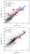 |
Fig. A.1. Star formation rate against stellar mass for GRB hosts and star-forming galaxies of the 3D-HST survey. Two redshift bins are considered, at 1 < z < 2 (top panel) and 2 < z < 3.1 (bottom panel). The star-forming galaxies selected in the analysis combining SFRUV+IR and SFRUV,corr values are plotted in background as a 2D gray histogram. The blue and dark blue curves are the main sequence relations derived by Whitaker et al. (2014) at 1 < z < 2.5. |
Appendix B: Comparison between methods to estimate the structural parameters
We sought to verify that our method of measuring GRB hosts structural parameters is consistent with the one of van der Wel et al. (2014) used for the reference sample. This ensures that no systematic bias is present when comparing GRB hosts and 3D-HST field galaxies. From the catalog of van der Wel et al. (2014), we considered all objects in the 3D-HST/GOODS-S field with a good fit (flag = 0). Among them, we randomly select ∼4 000 objects with 21 < HF160W < 28. We then ran our pipeline in a similar manner as described in Sect. 3.1.1. The pipeline failed for about 100 objects. The majority (75%) of them are not detected by our SExtractor configuration. The source extraction method used by van der Wel et al. (2014) is based on the "hot" and "cold" modes developed in GALAPAGOS. It is optimized to extract faint sources and properly deblended bright sources in mosaics. The undetected object are probably faint galaxies captured with the optimized source extraction algorithm of GALAPAGOS.
In Fig. B.1, we show the results for the half-light radius and the magnitude. We find a systematic offset of only ∼0.1 mag between the two magnitude estimates, and note that we also tend to systematically overestimate the half-light radius with our own procedure. At HF160W = 21.5 mag, we recover Re values within 10%, and the median offset then increases progressively with the magnitude until reaching 50% at HF160W = 26 mag. This behavior is not surprising since the accuracy of the fitting process depends to first order on the S/N and that the uncertainty in the background estimate becomes dominant at HF160W > 25.5 mag (van der Wel et al. 2012). However, the large majority (90%) of our GRB host sample is brighter than HF160W = 24 mag, i.e., where our fitting method reveals consistent results with the one used to estimate the Re in the 3D-HST catalog. We have only four objects with a magnitude higher than 25 that are excluded once the 3D-HST mass-completeness limit is applied. We thus conclude that these small offsets should have a negligible impact on our results. Finally, in Sect. 4, we emphasize that the sizes of GRB hosts measured with our code are globally smaller than the size of field sources from the 3D-HST catalog. Removing the systematic effect observed in Fig. B.1 would thus make this difference between the two populations even more significant, since our size determination tends to overestimate the sizes constrained by van der Wel et al. (2014).
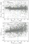 |
Fig. B.1. Comparison between F160W magnitudes (top panel) and half-light radii (bottom panel) derived by van der Wel et al. (2014) and our GALFIT modeling as a function of van der Wel et al. (2014) magnitudes. Each gray point represents an object of the 3D-HST/GOODS-S field. The gray curve is the median of the points and symbolizes the systematic offset for each parameter between the two methods. The vertical dashed blue line represents the maximum magnitude reached by GRB hosts above the 3D-HST mass-completeness limit, while our median H-band magnitude reaches ∼23.1 mag. |
Appendix C: GALFIT models of GRB hosts
In Figs. C.1, we show the best-fitting Sérsic profile derived by GALFIT for the sample of GRB hosts. In several cases (e.g., GRB 060814), multiple objects are fit simultaneously to reduce their contamination and improve the fitting process. Masked objects from the SExtractor segmentation map are visible as black areas. For the majority of cases, the residual maps show that we managed to remove the flux of the target object. To get a more quantitative indication of the fit goodness, a common method is to use the reduced χ2 returned by GALFIT. However, it can easily be misleading if the fitting process of nearby objects or the masking process is not properly performed. In order to have a better estimate of the remaining signal for each target object, we determined the fraction of pixels within 2 × Re that have a residual greater than three times the sigma map in the same area. The majority of the objects (33/35) have a residual fraction of ≲5% confirming the quality of the models considered. Only two objects (GRB 070306 and GRB 080605) have a residual fraction of ∼30%. Regarding GRB 080605, a plausible explanation is that the two nearby and bright stars probably contaminate the target object and thus interfere with the fitting process. For GRB 070306, the HST observations were performed several years after the GRB detection, thus excluding a possible contamination of the GRB afterglow that could affect the fitting process. We note that adding a PSF model in addition to the Sérsic model improves the fitting process and reduces the residuals to ∼10%. The resulting size determined by GALFIT evolves by a factor of 2 (from 0.14" to 0.28"). This may indicate an obscured active galactic nucleus or a recent burst of star formation in the host galaxy. Because these two objects represent only a small fraction of the total sample and the models appear realistic despite the large residual fraction, we decided to include them in our analysis. Finally, several objects (e.g., GRB 080207, GRB 111215A) would require more components to improve the residual maps. However, due to the constraint of using a single Sérsic component to model the objects, we did not add additional components to improve the residual maps.
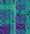 |
Fig. C.1. GRB hosts images from WFC3/F160W observations (left), their best GALFIT models (middle) and the residual maps (right). Images are centered on the best positions of the host galaxies determined by GALFIT and corresponds to a square region of 9 arcsec, where north is up and east is to the left. The red marks emphasize the objects considered as the GRB host galaxies. The black regions are the objects masked during the fitting processes based on the SExtractor segmentation map. The fraction of pixels with a residual greater than three times their noise within 2 × Re of the target object is visible in the lower part of the residual map. |
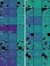 |
Fig. C.1. (continued) |
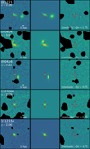 |
Fig. C.1. (continued) |
All Tables
All Figures
|
Fig. 1. Redshift cumulative distributions of our GRB host sample, compared to the host galaxies of unbiased GRB samples (SHOALS and BAT6). Objects are divided into two bins of redshifts. Top panel with GRB hosts at 1 < z < 2. Bottom panel with GRB hosts at 2 < z < 3.1. |
| In the text | |
|
Fig. 2. Stellar mass cumulative distributions of our GRB host sample, compared to the host galaxies of unbiased GRB samples (SHOALS and BAT6). Two bins of redshift are distinguished: with GRB hosts at 1 < z < 2 (top panel) and with objects at 2 < z < 3.1 (bottom panel). Upper limits are represented as arrows at the top of the plots. The 1σ uncertainty on the cumulative distribution is given by the shaded region around the curve. The p-value returned by the two-sided K–S test is provided in the right bottom part of both panels and color-coded according to the unbiased sample selected to compute the test. The vertical dashed line symbolizes the stellar mass completeness limit of the 3D-HST survey. |
| In the text | |
|
Fig. 3. Half-light radius of GRB hosts estimated by GALFIT in this work (x axis) compared to estimates based on SExtractor extracted from the literature (y axis). The FWHM of the PSF is visible as a gray dashed line. |
| In the text | |
|
Fig. 4. Compilation of stellar mass (top panel) and SFR (bottom panel) estimates for GRB hosts at 1 < z < 2. Each circle corresponds to an estimate from the literature or determined as described in Sect. 3.2. The circles marked with a star represent the estimates used in our analysis. |
| In the text | |
|
Fig. 5. Stellar mass of GRB hosts estimated from mass-to-light ratios, compared with the best estimates selected from the literature (Sect. 3.2). The residuals are shown in the bottom panel. Each GRB host is color-coded according to its redshift. The inset represents their associated F160W magnitude distribution (orange histogram) and the distribution of the GRB hosts for which no stellar mass measurement exists in the literature (red histogram). |
| In the text | |
|
Fig. 6. Size-mass relations and size deviations of GRB hosts from star-forming galaxies. Top panels: half-light radius against stellar mass for GRB hosts and star-forming galaxies at 1 < z < 2 (left panel) and 2 < z < 3.1 (right panel). The GRB host galaxies are displayed as red circles and the 3D-HST star-forming galaxies are shown as gray circles with an area proportional to their SFR. The median of the star-forming population is shown as a dashed gray line. The dashed cyan line represents the expected median of a GRB hosts population that does not suffer from bias to trace the SFR (gray circles weighted by their SFR). The 1σ uncertainty of the cyan median is given as a shaded cyan region. The vertical dashed black line is the mass-completeness limit of the 3D-HST survey. Bottom panels: cumulative distribution of Δ(Re − M∗) at 1 < z < 2 (left panel) and 2 < z < 3.1 (right panel). The Δ(Re − M∗) represents the distance between GRB hosts and the SFR-weighted Re − M∗ relation of the top panels. The blue curve is a Gaussian CDF with a mean of 0 and a standard deviation defined by the 1σ errors of the shaded cyan area at the GRB hosts positions. The p-value returned by the two-sided K–S test is provided in the right bottom part of panels. |
| In the text | |
|
Fig. 7. Stellar mass surface density (ΣM) against stellar mass for GRB hosts and star-forming galaxies (top panels) and cumulative distribution of Δ(ΣM − M∗) (bottom panels). The symbols are identical to those of Fig. 6. |
| In the text | |
|
Fig. 8. Star formation rate surface density (ΣSFR) against stellar mass for GRB hosts and star-forming galaxies (top panels) and cumulative distribution of Δ(ΣSFR − M∗) (bottom panels). Lower limits are represented as arrows and other symbols are identical to those of Fig. 6. |
| In the text | |
|
Fig. 9. Cumulative distributions as in Fig. 1 (top panel) and Fig. 2 (bottom panel) but showing the GRB host sample combined from Kelly et al. (2014) and Blanchard et al. (2016) at 0.3 < z < 1.1. |
| In the text | |
|
Fig. 10. Δ(Re − M∗) as a function of the redshift for GRB host galaxies. The orange and red circles are GRB hosts at z ≲ 1 from Kelly et al. (2014) and Blanchard et al. (2016), respectively. The blue circles are the GRB hosts considered in this study. Dark GRBs are highlighted by a thick black circle. The gray squares are the median of the Δ(Re − M∗) for each redshift bin. The associated error bars are the standard deviation using the MAD estimator. The black line at y = 0 represents the expected median values for a GRB hosts population that do not suffer from environment bias. |
| In the text | |
|
Fig. 11. Δ(ΣM − M∗) against redshift for GRB host galaxies. The symbols are identical to those of Fig. 10. |
| In the text | |
|
Fig. 12. Δ(ΣSFR − M∗) against redshift for GRB host galaxies. Lower limits are represented as arrows and other symbols are identical to those of Fig. 10. |
| In the text | |
|
Fig. A.1. Star formation rate against stellar mass for GRB hosts and star-forming galaxies of the 3D-HST survey. Two redshift bins are considered, at 1 < z < 2 (top panel) and 2 < z < 3.1 (bottom panel). The star-forming galaxies selected in the analysis combining SFRUV+IR and SFRUV,corr values are plotted in background as a 2D gray histogram. The blue and dark blue curves are the main sequence relations derived by Whitaker et al. (2014) at 1 < z < 2.5. |
| In the text | |
|
Fig. B.1. Comparison between F160W magnitudes (top panel) and half-light radii (bottom panel) derived by van der Wel et al. (2014) and our GALFIT modeling as a function of van der Wel et al. (2014) magnitudes. Each gray point represents an object of the 3D-HST/GOODS-S field. The gray curve is the median of the points and symbolizes the systematic offset for each parameter between the two methods. The vertical dashed blue line represents the maximum magnitude reached by GRB hosts above the 3D-HST mass-completeness limit, while our median H-band magnitude reaches ∼23.1 mag. |
| In the text | |
|
Fig. C.1. GRB hosts images from WFC3/F160W observations (left), their best GALFIT models (middle) and the residual maps (right). Images are centered on the best positions of the host galaxies determined by GALFIT and corresponds to a square region of 9 arcsec, where north is up and east is to the left. The red marks emphasize the objects considered as the GRB host galaxies. The black regions are the objects masked during the fitting processes based on the SExtractor segmentation map. The fraction of pixels with a residual greater than three times their noise within 2 × Re of the target object is visible in the lower part of the residual map. |
| In the text | |
|
Fig. C.1. (continued) |
| In the text | |
|
Fig. C.1. (continued) |
| In the text | |
Current usage metrics show cumulative count of Article Views (full-text article views including HTML views, PDF and ePub downloads, according to the available data) and Abstracts Views on Vision4Press platform.
Data correspond to usage on the plateform after 2015. The current usage metrics is available 48-96 hours after online publication and is updated daily on week days.
Initial download of the metrics may take a while.