| Issue |
A&A
Volume 664, August 2022
|
|
|---|---|---|
| Article Number | A187 | |
| Number of page(s) | 16 | |
| Section | Extragalactic astronomy | |
| DOI | https://doi.org/10.1051/0004-6361/202243930 | |
| Published online | 30 August 2022 | |
Dust emissivity in resolved spiral galaxies⋆
1
INAF – Osservatorio Astrofisico di Arcetri, Largo E. Fermi 5, 50125 Florence, Italy
e-mail: This email address is being protected from spambots. You need JavaScript enabled to view it.
2
INAF – Istituto di Radioastronomia, Via P. Gobetti 101, 40129 Bologna, Italy
3
AIM, CEA, CNRS, Université Paris-Saclay, Université Paris Diderot, Sorbonne Paris Cité, 91191 Gif-sur-Yvette, France
4
National Observatory of Athens, Institute for Astronomy, Astrophysics, Space Applications and Remote Sensing, Ioannou Metaxa and Vasileos Pavlou, 15236 Athens, Greece
5
Sterrenkundig Observatorium, Universiteit Gent, Krijgslaan 281 S9, 9000 Gent, Belgium
6
INAF – Istituto di Astrofisica Spaziale e Fisica Cosmica, Via Alfonso Corti 12, 20133 Milan, Italy
7
Space Telescope Science Institute, 3700 San Martin Drive, Baltimore, MD 21218-2463, USA
8
Université Paris-Saclay, CNRS, Institut d’Astrophysique Spatiale, 91405 Orsay, France
9
Department of Physics and Astronomy, N283 ESC, Brigham Young University, Provo, UT 84602, USA
Received:
3
May
2022
Accepted:
10
June
2022
Abstract
Context. The far-infrared (FIR) and sub-millimeter (submm) emissivity, ϵν, of the Milky Way (MW) cirrus is an important benchmark for dust grain models. Dust masses in other galaxies are generally derived from the FIR/submm using the emission properties of these MW-calibrated models.
Aims. We seek to derive the FIR/submm ϵν in nine nearby spiral galaxies to check its compatibility with MW cirrus measurements.
Methods. We obtained values of ϵν at 70–500 μm, using maps of dust emission from the Herschel satellite and of gas surface density from the THINGS and HERACLES surveys on a scale generally corresponding to 440 pc. We studied the variation of ϵν with the surface brightness ratio Iν(250 μm)/Iν(500 μm), a proxy for the intensity of the interstellar radiation field heating the dust.
Results. We find that the average value of ϵν agrees with MW estimates for pixels sharing the same color as the cirrus, namely, for Iν(250 μm)/Iν(500 μm)=4.5. For Iν(250 μm)/Iν(500 μm)> 5, the measured emissivity is instead up to a factor ∼2 lower than predicted from MW dust models heated by stronger radiation fields. Regions with higher Iν(250 μm)/Iν(500 μm) are preferentially closer to the galactic center and have a higher overall (stellar+gas) surface density and molecular fraction. The results do not depend strongly on the adopted CO-to-molecular conversion factor and do not appear to be affected by the mixing of heating conditions.
Conclusions. Our results confirm the validity of MW dust models at low density, but are at odds with predictions for grain evolution in higher density environments. If the lower-than-expected ϵν at high Iν(250 μm)/Iν(500 μm) is the result of intrinsic variations in the dust properties, it would imply an underestimation of the dust mass surface density of up to a factor ∼2 when using current dust models.
Key words: dust, extinction / infrared: galaxies / galaxies: photometry / galaxies: ISM
This work makes use of the DustPedia database. DustPedia is a collaborative focused research project supported by the European Union under the Seventh Framework Programme (2007–2013) call (proposal no. 606824, P.I. J. I. Davies). The database is publicly available at http://dustpedia.astro.noa.gr.
© S. Bianchi et al. 2022
 Open Access article, published by EDP Sciences, under the terms of the Creative Commons Attribution License (https://creativecommons.org/licenses/by/4.0), which permits unrestricted use, distribution, and reproduction in any medium, provided the original work is properly cited.
This article is published in open access under the Subscribe-to-Open model. This email address is being protected from spambots. You need JavaScript enabled to view it. to support open access publication.
1. Introduction
Since the 1980s, a variety of satellites have carried out detailed studies of the thermal emission of dust grains in the Milky Way (MW), from its far-infrared (FIR) peak down to the submillimeter (submm) and longer wavelengths. In particular, observations of dust have been compared with those of hydrogen emission lines in order to derive the dust emissivity, ϵν, that is, the surface brightness per H column density (see, e.g., Boulanger et al. 1996; Dwek et al. 1997; Planck Collaboration Int. XVII 2014). Besides the optical properties, size distribution, material composition, grain shape, and abundance, ϵν depends on the intensity of the interstellar radiation field (ISRF) heating the dust grains. For clouds at high Galactic latitude, that is, the so-called cirrus (Low et al. 1984), the starlight intensity is well known from observations and the local ISRF (LISRF; Mathis et al. 1983) can be used to estimate the temperatures attained by grains of different materials and radii. Thus, the MW cirrus emissivity has become a benchmark in defining the absorption (emission) cross-section of the dust grain mixtures (see Hensley & Draine 2021 for a recent review on ϵν and other observational constraints for dust models).
Models of the MW dust, such as those of Zubko et al. (2004), Draine & Li (2007), and The Heterogeneous dust Evolution Model for Interstellar Solids (THEMIS; Jones et al. 2013, 2017) are routinely applied to FIR-submm observations of other galaxies in order to extract various information. Such data include, for example, the amount of dust mass and the heating contribution from young stars, providing clues on the evolution of the metals constituting the grains and extinction-free estimates of the star formation rate. Several works use MW dust models to fit the dust emission spectral energy distribution (SED) in galaxies, among them (Hunt et al. 2019; Nersesian et al. 2019; Aniano et al. 2020, and Galliano et al. 2021). The works cited above make use of data from the Herschel Space Observatory (Pilbratt et al. 2010), which has considerably improved the knowledge of the FIR-to-submm SED of galaxies, thanks to the mapping capabilities of the Photodetector Array Camera and Spectrometer (PACS; Poglitsch et al. 2010), and the Spectral and Photometric Imaging Receiver (SPIRE; Griffin et al. 2010).
The question that remains is whether MW dust is representative of the average grain properties in other galaxies. A first test was attempted by James et al. (2002), who derived the disk-averaged dust absorption cross-section in nearby spirals, using estimates of the mass available in metals to infer the dust mass independently from FIR-submm observations. In a similar fashion, Clark et al. (2016) and Bianchi et al. (2019) used Herschel global photometry and found results that are generally consistent with the MW properties, with a large scatter, however. Applying the same method pixel-by-pixel to Herschel maps of two galaxies, Clark et al. (2019) reported variations of the absorption cross-section with the environment, with smaller absorption cross-sections for pixels characterized by larger interstellar medium (ISM) densities, apparently at odds with models of the evolution of dust in denser environments (e.g., Köhler et al. 2015).
However, the process of estimating the dust mass (or surface density in resolved analysis) from metals, following the method of James et al. (2002), is subject to several uncertainties: (i) the total gas column density is needed, which relies on the recipe used to derive its molecular component, typically from observations of CO lines; (ii) an estimate of the dust-to-gas mass ratio must be inferred from metallicity measurements, from solar or local ISM values, taking into account the observed metal depletions; (iii) a functional form needs to be assumed for the cross section (a power law) and a single temperature is estimated from fitting the SED, thus basically assuming that dust grains have the same properties everywhere in a galaxy. Indeed, Priestley & Whitworth (2020) have suggested that the result of Clark et al. (2019) could be biased by dust at colder temperatures, which is expected in denser environments because there the ISRF is attenuated by dust extinction. This colder dust would be unaccounted for in a single-temperature fit.
To overcome these uncertainties, Bianchi et al. (2019) suggested limiting the analysis to the emissivity, ϵν, for which no temperature derivation and dust-to-gas prescription are needed; it is only the uncertainty in the derivation of the molecular gas from CO that remains. The emissivity ϵν can then be compared with the response of a dust model (obtained either from fitting the MW cirrus data or after following the evolution of grains in different environments) to ISRFs of different intensities. For their sample of 204 objects, Bianchi et al. (2019) found an average emissivity similar to that measured in the MW, for the same FIR color as in the cirrus, and a reduction in emissivity (with respect to model predictions) for galaxies with more intense ISRF and a larger contribution of molecular gas to the ISM (thus, similarly to that found by Clark et al. 2019, given that higher molecular fractions tends to be closely associated with higher gas surface densities). The dependence on the interstellar environment could only be studied indirectly by Bianchi et al. (2019), however, since a single global emissivity was derived for each object.
Improving on the work of Bianchi et al. (2019), here we derive the emissivity using dust emission and gas column density maps for a sample of nine low-inclination spirals. These objects are among the largest and nearest galaxies observed by Herschel and are thus included in the DustPedia sample (Davies et al. 2017). The aim of the analysis is to verify, on a resolved scale, the general validity of the MW dust model for other galaxies and to assess possible variations of the dust properties across galactic disks.
The paper is organized as follows: in Sect. 2, we describe the sample and dataset we use. The emissivity derivation is presented in Sect. 3. Results on ϵν(250 μm) are shown in Sect. 4 and discussed in Sect. 5. The emissivity SED is described in Sect. 6. In Sect. 7, we summarize the results and present our conclusions.
2. Sample and dataset
Our sample is drawn from the work of Casasola et al. (2017), who selected the largest low-inclination spiral galaxies in DustPedia (18 objects more extended than 9′ in SPIRE images) and study the spatial distribution of stellar emission, dust emission, gas column density, and other derived quantities. Among these, we chose objects that have both observations of atomic and molecular gas from homogeneous sources. We retained 9 galaxies: they are listed in Table 1.
Properties of the sample.
Herschel dust continuum images from PACS at 70, 100 and 160 μm and from SPIRE at 250, 350 and 500 μm were taken from the DustPedia database (Clark et al. 2018). Map resolutions range from FWHM ≈ 9″ at 70 μm to 36″ at 500 μm. The majority of galaxies have the full FIR/submm wavelength coverage, with the exceptions of NGC 2403 and NGC 5194, which were not observed at 100 μm. As in Casasola et al. (2017), we used sky areas outside the targets to estimate the instrumental and confusion noise.
Maps of the H I column density were obtained from 21 cm line observations undertaken at the Very Large Array of the National Radio Astronomy Observatory, within The HI Nearby Galaxy Survey (THINGS; Walter et al. 2008). We used the ROBUST dataset, providing a uniform synthesized beam with FWHM ≈ 6″. The original moment 0 maps (and their estimated noise) were converted into units of column density with the usual assumption of optically thin H I emission.
To trace the molecular gas column density, we used the moment 0 maps (and error maps) from the HERA CO-Line Extragalactic Survey (HERACLES; Leroy et al. 2009), which observed the 12CO(2-1) line at the IRAM 30 m telescope with resolution FWHM = 11″.
We smoothed all images to the lowest resolution of the dataset, namely, FWHM = 36″ at 500 μm. We used the convolution kernels of Aniano et al. (2011): for Herschel maps, kernels are available to pass from the original point spread function (PSF) to that at 500 μm; for gas column density maps, we assumed that the original PSF is a Gaussian of appropriate size. All maps were regridded to a common grid of pixel size 12″ (the pixel scale of SPIRE 500 μm images in DustPedia, equivalent to FWHM/3).
As detailed in the next section, we applied metallicity and column density-dependent CO-to-H2 conversion factors: for this, we used the O/H metallicity gradients provided by Pilyugin et al. (2014, see Appendix A for a justification) and the stellar surface density maps derived by Casasola et al. (2017). For each galaxy, the total surface density was derived by adding together the stellar and gas contribution (with the usual 36% correction to include He and other metals in the gas budget), and de-projecting the maps using the inclinations listed in Table 1. We also used NUV maps from the GALaxy Evolution eXplorer (GALEX; Morrissey et al. 2007) and 3.6 μm maps from the InfraRed Array Camera (IRAC) aboard the Spitzer Space Telescope (Werner et al. 2004), available from the DustPedia database; these were corrected for foreground MW extinction as in Clark et al. (2018).
3. Method
For the MW cirrus, the dust emissivity ϵν is defined as the surface brightness of dust emission Iν per hydrogen column density NH. For each pixel considered in our analysis, we estimated the emissivity accordingly, using
 (1)
(1)
While the column density of atomic gas can be derived directly from observations of the 21 cm H I line, NH2 can only be estimated indirectly: typically, the lines of CO are used, as they are considered the main tracer of molecular gas. Here, since we are using the intensity of the CO(2-1) line, we can write:
 (2)
(2)
where R21 = ICO(2−1)/ICO(1−0) is the ratio between the intensities of the (2-1) and (1-0) lines, and XCO is the CO-to-H2 conversion factor, normally derived for the CO(1-0) line.
To maintain a consistency with Bianchi et al. (2019), where molecular masses from Casasola et al. (2020) are used, here we adopt R21 = 0.7, a typical value found in the MW disk and in some HERACLES galaxies (Leroy et al. 2013). This value is consistent with the recent determination of den Brok et al. (2021), who found an average R21 = 0.63 with a scatter of 15%, on a sample of nine nearby galaxies (four of which in our sample), as well as with Leroy et al. (2022), who have R21 = 0.65 and a scatter of 30% on a larger sample of 43 objects (seven in common with ours). Both works find evidence of a possible increase of R21 in denser environments, and also find that the scatter is dominated by galaxy-to-galaxy variations.
For the conversion factor, studies of molecular clouds in the MW disk have found:
 (3)
(3)
which is estimated to have an uncertainty of 30% (Bolatto et al. 2013). The XCO factor is supposed to increase in lower metallicity environments, because of the reduced availability of the CO molecule and because of reduced shielding against its photodissociation in less dusty clouds; instead, it should drop in higher density regions, such as galactic centers, where the gas temperature is higher. Based on observations and theoretical models, Bolatto et al. (2013) propose a metallicity and surface-density-dependent conversion factor, which can be written as:
 (4)
(4)
with γ = 0.5 for a total surface density (stars+gas) Σtotal > 100 M⊙ pc−2 and γ = 0 otherwise; the metallicity derived from (O/H) by using log10(Z/Z⊙)=12 + log10(O/H)−8.69, so that log10(Z/Z⊙)=0 for the MW disk environment (assuming it follows the Solar mixture). Equation (4) further assumes that the characteristic surface density of molecular clouds in a galaxy and in the MW is the same and equal to 100 M⊙ pc−2 (see also Chiang et al. 2021).
Other works based on large galaxy samples suggest a power-law dependence of XCO on global metallicity. In those studies, the power-law index is derived by imposing that the molecular mass must correlate with the star formation rate, for all metallicities. One such work is Hunt et al. (2020), who found:
 (5)
(5)
A similar power-law index was found by Amorín et al. (2016; this is used by Bianchi et al. 2019), although steeper metallicity dependences have also been found (Hunt et al. 2015; Madden et al. 2020).
In this work, we assume the  conversion factor. We also comment on the variation of the emissivity when
  and
and  are used; we warn, thought, that the latter was derived on global galactic properties and not on a resolved scale.
We did not include the contribution of H II to NH: this is normally neglected in the derivation of the MW emissivity and it is not included in the estimate of the average emissivities of DustPedia galaxies also (for a discussion, see Bianchi et al. 2019).
4. Results
For each galaxy in the sample, we derived the emissivity in all Herschel bands, using Eq. (1). Following Bianchi et al. (2019), we conduct our analysis as a function of Iν(250 μm)/Iν(500 μm), which, for standard models of dust emission, is directly related to the intensity of the starlight heating the dust grains (see Appendix B). Given Eq. (1), Iν(250 μm)/Iν(500 μm) is equivalent to ϵ(250 μm)/ϵ(500 μm). We used all pixels with S/N > 3 in the Iν(250 μm)/Iν(500 μm) maps, defining a contiguous large area for each galaxy and allowing for the selection of high-quality data for all the other quantities we analyze here. In total, the whole sample consists of about 13 600 pixels. The contribution of each galaxy to the available pixels depends on its physical dimension and distance, but also on the limited coverage of the CO data for some objects. In Fig. 1 we show the dataset, ϵν(250 μm), and Iν(250 μm)/Iν(500 μm) for NGC 5457, the largest galaxy we analyze, contributing more than one-third of the available pixels (see Table 1). Maps for ϵν(250 μm) with contours for Iν(250 μm)/Iν(500 μm) for the other galaxies of the sample are presented in Fig. 2.
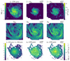 |
Fig. 1. Dataset and results for NGC 5457. The top row shows the 250 μm image, the molecular gas column density derived from CO observations for |


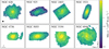 |
Fig. 2. Maps of ϵν(250 μm) for the rest of the sample (assuming |

In Fig. 3, we show ϵν(250 μm) as a function of Iν(250 μm)/Iν(500 μm), for all the pixels (left panel) and as contours of the pixel density (right panel). As expected, ϵν(250 μm) grows with Iν(250 μm)/Iν(500 μm), as also found by Bianchi et al. (2019) for galaxy integrated values. In the left panel, we plot the mean value of ϵν(250 μm) for each galaxy, after binning the pixels in five equal bins of Iν(250 μm)/Iν(500 μm) in the range: [3,8]. Individual objects have their own trend. In addition, not all galaxies cover the full set of bins: NGC 5457 and NGC 628 have pixels spanning the whole Iν(250 μm)/Iν(500 μm) range; in NGC 925 and NGC 2403 most of the pixels falls in the first two color bins; the rest of the galaxies, instead, privileges the higher Iν(250 μm)/Iν(500 μm) values (see also the contour in Fig. 2).
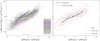 |
Fig. 3. Emissivity at 250 μm, ϵν(250 μm) versus the Iν(250 μm)/Iν(500 μm) ratio (assuming |

The average ϵν(250 μm) of the whole sample is shown by the solid black line in the right panel of Fig. 3: as in Bianchi et al. (2019), we used the mean of all pixels within each bin (without any weighting). The trend does not appear to be influenced strongly by a particular behavior of an individual galaxy: for example, it does not change significantly when we exclude the dominant contribution from NGC 5457 (dashed black line). We also checked the impact of the different spatial scales of our galaxies: they range from 190 pc, for NGC 2403, to 720 pc, for NGC 3521 (for the adopted angular scale of 12″; Table 1). The average spatial scale over the whole pixel sample is 440 pc. Despite the wide range, a large fraction of the available pixels (≈70%) belongs to five galaxies with scales within 25% of the average; the other four galaxies are the two nearest and two farthest ones. If we restrict the analysis to the five galaxies with more uniform spatial scales, the average ϵν(250 μm) trend is almost indistinguishable from that of the whole sample: thus, 440 pc can be considered the characteristic physical scale of our analysis. Because of this, we have preferred to keep a fixed angular scale grid (as also done in other works; see, e.g., Sandstrom et al. 2013; Jiao et al. 2021), rather than to degrade all the scales to that of farthest object and significantly reduce the number of pixels.
The scatter around the mean values in Fig. 3 is reduced with respect to that in Bianchi et al. (2019): for the bin centered at Iν(250 μm)/Iν(500 μm)=4.5, it is ≈40% and ≈30% for Iν(250 μm)/Iν(500 μm)=7.5. Instead, it was larger for the integrated analysis, namely ≈50% in all bins. The reduction in scatter is likely due to the more homogeneous dataset in the current work. Bianchi et al. (2019) rely on gas observations gathered from several sources in the literature, with gas masses (and thus average surface densities) obtained after applying general recipes for aperture corrections (in particular for H2 masses, the majority of which were derived from observations of the sole galactic centre; see Casasola et al. 2020).
Part of the scatter in Fig. 3 is due to photometric errors: for Iν(250 μm)/Iν(500 μm), the average uncertainty is ≈0.5 for the first three bins, and ≈0.4 for the last two; it rises to ≈0.5−0.6 when the calibration error is taken into account (using the fraction of it which is uncorrelated among the SPIRE bands, see Appendix A in Galliano et al. 2021). This justifies the choice of averaging over bins of width ΔIν(250 μm)/Iν(500 μm)=1. The average error on ϵν(250 μm) is instead a few percent (plus an additional 6% when the calibration error at 250 μm is included; Galliano et al. 2021). The average ϵν(250 μm) and Iν(250 μm)/Iν(500 μm) errors for the central bin are shown in the left panel of Fig. 3. In order to test the effects of these uncertainties on the pixel distribution in the ϵν(250 μm)-Iν(250 μm)/Iν(500 μm) plane, we made a simulation assuming that the average trend in Fig. 3 is the “exact” behavior of emissivity in all galaxies. For each pixel, we used the measured Iν(250 μm) to derive a mock Iν(500 μm) according to the “exact” trend. From both flux densities we then extracted random values, adopting Gaussian errors and the measured uncertainty for that pixel (but neglecting calibration errors). The same was done for NH (neglecting the uncertainties in the CO-to-H2 conversion factor, which will be discussed later). Finally, mock realizations of ϵν(250 μm) and Iν(250 μm)/Iν(500 μm) according to this “exact” hypothesis were produced: one of them is shown with red contours in the right panel of Fig. 3. From this test, we obtain the result that photometric uncertainties alone can produce a scatter in ϵν(250 μm) of about 20%, because of the shuffling due to the large bin (and uncertainties) in Iν(250 μm)/Iν(500 μm), and of the ϵν(250 μm) uncertainties themselves. After subtracting this contribution, we conclude that there is an intrinsic scatter in ϵν(250 μm) of ≈35% and 20% (at Iν(250 μm)/Iν(500 μm)=4.5 and 7.5, respectively) due to pixel-by-pixel and object-by-object variations in the dust properties. The fact that scatter is not only due to statistical errors is also indicated by the differences between the individual galaxy averages as well as between those averages and the whole sample average: these are much larger than the standard error of the mean (not shown, being smaller than the symbol size used for the average trends in Fig. 3).
The random procedure of the previous paragraph was also used to check to what extent the trend seen in Fig. 3 is induced by the use of the same quantity, Iν(250 μm), in the derivation of both ϵν(250 μm) and Iν(250 μm)/Iν(500 μm). In fact, when non-independent quantities are plotted, spurious correlations might arise because of the uncertainties (see, e.g., Mosenkov et al. 2014; De Vis et al. 2017). We checked this by adopting a “null” hypothesis, namely, that there is no correlation between Iν(250 μm) and Iν(250 μm)/Iν(500 μm), and thus between Iν(250 μm) and Iν(500 μm); this was done by shuffling the pixel values within the 500 μm maps. Indeed, we found that a spurious correlation can arise between ϵν(250 μm) and Iν(250 μm)/Iν(500 μm) and we show the average trend with a dashed blue line in the right panel of Fig. 3. However, this trend is much fainter than what is actually found in the data. Indeed, a physical connection between Iν(250 μm)/Iν(500 μm) and ϵν(250 μm) is expected: in a warmer radiation field, dust is heated to higher temperatures and Iν(250 μm)/Iν(500 μm) should increase; at the same time, under the thermal emission hypothesis, both Iν(250 μm) and Iν(500 μm) (and the related emissivities), should grow.
We also studied the dependence of the ϵν(250 μm)−Iν(250 μm)/Iν(500 μm) correlation on other quantities available through the DustPedia archive and previous analysis. For each galaxy, both ϵν(250 μm) and Iν(250 μm)/Iν(500 μm) are higher in regions where the optical-NIR stellar emission, the gas column density, and the metallicity are higher. However, we did not find any quantity that could be associated with a galaxy’s individual trend in the ϵν(250 μm)−Iν(250 μm)/Iν(500 μm) plane. Thus, in the following, we will only discuss the general trend for the whole of the sample. In Fig. 4 we show, on the ϵν(250 μm)−Iν(250 μm)/Iν(500 μm) plane, the average values for the stellar mass surface density Σ⋆, the UV-to-NIR ratio SNUV/S3.6 μm, the fraction of molecular gas fmol = 2 × NH2/NH, and the gas mass surface density ΣISM.
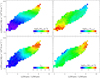 |
Fig. 4. ϵν(250 μm) versus Iν(250 μm)/Iν(500 μm), same grey contours as in Fig. 3. In each panel, the color map shows the average value of the following quantities: Σ⋆, SNUV/S3.6 μm, fmol and ΣISM. |
The quantity that correlates most with ϵν(250 μm) and Iν(250 μm)/Iν(500 μm) is Σ⋆: the non-parametric Spearman’s test gives a correlation coefficient ρ = 0.93 for Σ⋆ versus ϵν(250 μm) and ρ = 0.89 for Σ⋆ versus Iν(250 μm)/Iν(500 μm) (in all cases discussed here, the correlations are significant at a confidence level > 99.99%). As a comparison, ϵν(250 μm) and Iν(250 μm)/Iν(500 μm) are correlated among themselves with ρ = 0.86. Besides being used in Eq. (4), Σ⋆ can also be considered as a proxy for the optical-NIR ISRF: thus, dust in regions with higher Σ⋆ have higher Iν(250 μm)/Iν(500 μm) and ϵν(250 μm). Instead, the UV ISRF appears to contribute less to the dust heating. This is shown by the anticorrelation between SNUV/S3.6 μm and ϵν(250 μm), with ρ = −0.55 (ρ = −0.67 for Iν(250 μm)/Iν(500 μm)). We found that one galaxy, NGC 3521, characterized by a low global SNUV/S3.6 μm (≈0.02, using data from Clark et al. 2018) also has low ϵν(250 μm) for Iν(250 μm)/Iν(500 μm)=5−6 (see the left panel of Fig. 3). Pixels from this galaxy are responsible for lowering slightly the average SNUV/S3.6 μm in Fig. 4, on the low-emissivity side of the outer contour plot. However, this does not seem to be a general property of other galaxies of lower UV emission: for example, NGC 4736 and NGC 5055, with global SNUV/S3.6 μm ≈ 0.03, and NGC 5194, with SNUV/S3.6 μm ≈ 0.06, follow the mean trend with the other galaxies (all with global SNUV/S3.6 μm ≳ 0.1).
Strong correlations are also found for fmol, with Spearman’s ρ = 0.81 with respect to ϵν(250 μm) and ρ = 0.85 with respect to Iν(250 μm)/Iν(500 μm). For ϵν(250 μm) versus fmol, the correlation could, in principle, be boosted by the fact that both quantities depend on 1/NH; yet the errors on gas column density are small and indeed a test shows a null correlation if we assume that the 250 μm surface density is completely uncorrelated to the gas column density (we used the same random procedure as for the “null” test, this time by shuffling the pixel values for the gas column density). The enhancement of emissivity in regions with higher molecular gas fraction is in agreement with Bianchi et al. (2019), where the same result is found for mean galactic properties. This behavior translates, with some scatter and a reduction in the correlation, to that for ΣISM, where it is ρ = 0.52 with respect to ϵν(250 μm) and ρ = 0.63 with respect to Iν(250 μm)/Iν(500 μm). In general, ΣISM is larger for higher Iν(250 μm)/Iν(500 μm) values. For Iν(250 μm)/Iν(500 μm)< 5, there also seems to be a trend of higher ϵν(250 μm) for pixels with a lower column density. However, this is a spurious effect due to the dependence of ϵν(250 μm) on 1/NH: in this range, the “noisier” pixels in Iν(250 μm)/Iν(500 μm) determine a roughly constant lower limit in I(250μm), regardless of their gas column density; thus ϵν(250 μm) is boosted in pixels of lower ΣISM (belonging mostly to NGC 5457).
Overall, Iν(250 μm)/Iν(500 μm) and ϵν(250 μm) are higher in the central regions of a galaxy, where the stellar and total gas surface density, as well as the molecular gas contribution to the ISM (along with metallicity, for which we used a smooth negative gradient) are high, and the UV radiation field is reduced with respect to the optical-NIR. Indeed, for each galaxy, strong inverse correlations are found with the galactocentric distance, d: for example, the Spearman’s correlation coefficient for ϵν(250 μm) versus d ranges from ρ = −0.83 for NGC 5194 to −0.97 for NGC 5055. When the whole sample is considered, and the distances scaled on the optical radii of each galaxy, the correlation is reduced, with ρ = −0.61 for ϵν(250 μm) versus d/R25. This may be due to the fact that a simple scaling on R25 is not able to describe the relevant gradients in physical conditions. In fact, when scaling the distance on the stellar scalelength h⋆ from Casasola et al. (2017), which at least captures the variation in the stellar surface density of the disk (but not of the central parts of a galaxy), the correlation for ϵν(250 μm) versus d/h⋆ is raised to ρ = −0.73. In any case, the enhancement of ϵν(250 μm) with radiation field and gas density is dominated by the smooth galactic gradient. A possible effect along spiral arms is instead not evident in our analysis, because of their smaller dynamic range and because of the low resolution imposed by the 500 μm data, resulting in the lack of an evident trace of spiral arms in the Iν(250 μm)/Iν(500 μm) maps (as shown by Figs. 1 and 2).
5. Discussion
The average emissivity in the Iν(250 μm)/Iν(500 μm)=4.5 bin is very close to the value found for the high-latitude Galactic cirrus, ϵν(250 μm)=0.79 ± 0.07 MJy sr−1 (1020 H cm−2)−1 for Iν(250 μm)/Iν(500 μm)=4.6 ± 0.6 (Fig. 5; see Bianchi et al. 2017, 2019 for the MW estimate1). This reassures on the use of the MW emissivity to derive dust masses in other galaxies: as shown in the previous section, the intrinsic scatter around this value is limited to 35%. The scatter possibly hides variations in the dust properties within a galaxy and from object to object, even though we could find no clear dependence on any measurable quantity.
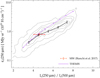 |
Fig. 5. ϵν(250 μm) versus Iν(250 μm)/Iν(500 μm). Comparison between our results and the MW value for the cirrus. We also show the behavior of the THEMIS dust model under ISRFs of growing intensities (dots are for U = 0.2, 0.5, 1, 2, 5, 10, 20, and 50 from left to right, with ISRF = U × LISRF; see Appendix B). Grey contours and average emissivity as in Fig. 3. The errorbars for the average emissivity show the impact on ϵν(250 μm) of the SPIRE calibration error. |
For the expected values of ϵν(250 μm) at different Iν(250 μm)/Iν(500 μm), we have to rely on dust grain models. In Fig. 5, we show the behavior of the THEMIS model for diffuse dust under varying intensities of the ISRF heating the grains (from less to more intense ISRFs, from left to right; see Appendix B for details on the calculation). For Iν(250 μm)/Iν(500 μm)≲5 the dust model follows the average trend of the data, within the SPIRE 250 μm calibration uncertainty. Indeed, THEMIS is made to pass from the MW emissivity estimate when the heating field is the LISRF (the dot with U = 1 in Fig. 5). However, for Iν(250 μm)/Iν(500 μm)≳5 the THEMIS prediction overestimates the average emissivity: for Iν(250 μm)/Iν(500 μm)=5.5, 6.5, 7.5, the average ϵν(250 μm) is a factor 1.4, 1.7 and 1.9 lower, respectively, than the expectation for the model at the same color ratios, while we found a total scatter of 30% only (including photometric uncertainties). A similar discrepancy is found in Bianchi et al. (2019).
The most naive interpretation of the tension between our estimates and the theoretical predictions is that the lower ϵν(250 μm) for higher Iν(250 μm)/Iν(500 μm) is simply due to a reduction in the dust absorption cross section with respect to that of THEMIS. If this is true, the dust mass surface density for pixels with Iν(250 μm)/Iν(500 μm)≳5 could be underestimated by up to a factor ≈2, when using the dust properties from the model. The impact of this underestimation on the global dust mass in a galaxy would depend on the fraction of the dust emission at higher Iν(250 μm)/Iν(500 μm). We tested this by using the dust maps obtained using THEMIS in Casasola et al. (2017) and raising the dust surface density for the pixels in the three higher Iν(250 μm)/Iν(500 μm) bins, by the average factors discussed in the previous paragraph. For two galaxies, the total dust mass after this correction is within 10% of the original estimate: they are NGC 925 and NGC 2403 which (as we have seen) have a dearth of pixels with Iν(250 μm)/Iν(500 μm)> 5. For the other galaxies, the corrected dust mass would be from 35 to 55% higher, with the exception of NGC 5194, where it would rise by 75%.
However, there are other possible explanations for the lower-that-expected ϵν(250 μm) at higher Iν(250 μm)/Iν(500 μm), apart from global variations in the dust properties. We explore them in the rest of this section.
5.1. ISRF mixing
The predictions of Fig. 5 rely on the simplifying assumption that all of the dust is heated by a homogeneous ISRF. However, along any line of sight (i.e., the pixel level in our analysis) dust might be subject to a range of heating conditions with, for example, most of the grains absorbing light from a less intense ISRF, and a fraction of them being heated to higher temperatures in a more intense field. Indeed, when a dust grain mixture is exposed to a distribution of ISRFs, the resulting spectrum is broader: this might alter the position and trend of the model predictions in the ϵν(250 μm)−Iν(250 μm)/Iν(500 μm) plane.
We explore the effects of this mixing of heating conditions in Appendix B, by testing the ISRF distributions which are typically used to fit the global or resolved SED of galaxies. In general, we found that the effects of ISRF mixing are small, at least when emission at longer wavelength is concerned: the trends we found are not much different from the case of homogeneous ISRF shown in Fig. 5. A moderate bias could be present for Iν(250 μm)/Iν(500 μm)=4.5, with ϵν(250 μm)∼10% lower (at maximum) than the values from a single intensity ISRF. However, the difference reduces for higher Iν(250 μm)/Iν(500 μm) and cannot explain the lower values for ϵν(250 μm) we find.
Another simplification in the modeling of dust heating is to assume always the same spectral shape for starlight, namely, that of the LISRF. Instead, dust could be heated by UV-dominated ISRFs near star-forming regions or by a redder spectrum in the diffuse medium close to the center of galaxies. Nevertheless, we found that the use of different spectra does not significantly change the modeled trends in the ϵν(250 μm)−Iν(250 μm)/Iν(500 μm) plane (Appendix B).
5.2. Dust in different environments
Clark et al. (2019) used Herschel maps of two galaxies (one of which, NGC 628, is also included in our sample) to derive the dust absorption cross section, after having estimated the total dust mass from gas and metallicity measurements. They reported a reduction of the dust absorption cross-section for lines of sight of higher ΣISM. While we do not derive the absorption cross-section in this work and limit our analysis to the emissivity only, we support a similar view: pixels with Iν(250 μm)/Iν(500 μm)> 5, where the average ΣISM is higher (see Fig. 4), have a reduced ϵν(250 μm), with respect to model predictions.
In dense environments dust grains are expected to accrete atoms from the ISM, develop ice mantles, and coagulate: all these processes tend to increase the absorption cross-section (and emissivity) rather than decrease it (see, e.g., Köhler et al. 2015). In Bianchi et al. (2019) we tested the results of Köhler et al. (2015) and confirmed that, even for the less evolved grain mixture studied in that work (the CMM model), ϵν(250 μm) is higher than what expected for diffuse dust. Furthermore, the evolution of dust grain properties is supposed to occur in regions where the ISRF is shielded, and thus at lower Iν(250 μm)/Iν(500 μm), while we find a discrepancy with the diffuse dust model at larger Iν(250 μm)/Iν(500 μm).
Priestley & Whitworth (2020) suggest that the results of Clark et al. (2019) are biased: along the lines of sight with higher column density, emission from dust exposed to the ISRF in the diffuse medium could be mixed with emission coming from dense molecular clouds; here, grains attain a lower temperature because they are reached by a lower intensity ISRF, attenuated by extinction from dust itself. Neglecting the presence of colder dust and using a single temperature to model the SED, as done by Clark et al. (2019), results in a lower estimate of the absorption cross sections, essentially because colder dust contributes only minimally to the overall emission (while it is accounted for in the dust mass estimated from the gas metallicity). In Appendix B, we tested the impact on our estimates of the scenario proposed by Priestley & Whitworth (2020). We found that ϵν(250 μm) could be biased low by a significant amount only for the higher ΣISM we found in our sample, and in particular for lower intensity ISRFs. Instead, the bias is smaller for the more intense ISRFs that should be responsible for the emission at larger Iν(250 μm)/Iν(500 μm). In fact, even assuming different properties for dust in denser environments (the CMM model of Köhler et al. 2015), the trend of ϵν(250 μm) versus Iν(250 μm)/Iν(500 μm) is not substantially altered from that predicted for single-ISRF models. The bias described by Priestley & Whitworth (2020) cannot thus explain the discrepancy between model expectations and ϵν(250 μm) estimates at Iν(250 μm)/Iν(500 μm)> 5.
5.3. Dependence on XCO
So far, we only considered the uncertainties due to photometry. However, there are also large uncertainties in the CO-to-H2 conversion factor. We estimated them for  , using a Monte Carlo procedure and building random representations of the ϵν(250 μm) versus Iν(250 μm)/Iν(500 μm) distribution according to the scatter in
  and R21 described in Sect. 3 (and to the scatter in the metallicity gradients from Pilyugin et al. 2014, although this is a minor effect; see also Appendix A for the impact of different metallicity calibrators). Since the uncertainty in
  is common to all galaxies, we draw a single random value for this quantity in each representation, while we draw independent values of R21 for each galaxy (thus assuming that the measured scatter is due to galaxy-to-galaxy variations; we used the estimate of Leroy et al. 2022). After running a thousand representations, we measured the standard deviation of the random ϵν(250 μm) trends, shown by the shaded area in Fig. 6. At Iν(250 μm)/Iν(500 μm)=4.5, the uncertainty due to
  is 8%, much smaller than the scatter in the dataset: this is the reflection of the very low contribution of molecular gas to NH and thus on the little dependence of ϵν(250 μm) on XCO for the first Iν(250 μm)/Iν(500 μm) bins. For larger Iν(250 μm)/Iν(500 μm), instead, the contribution of molecular gas increases (see fmol in Fig. 4) and the uncertainty in ϵν(250 μm) due to the CO-to-H2 conversion factor grows: at Iν(250 μm)/Iν(500 μm)=7.5 it is 30%, the same as the scatter in the observations. Even combining this uncertainty with the data scatter, the difference between the observed ϵν(250 μm) and the model cannot be explained.
5.3.1. Different XCO recipes
The ϵν(250 μm) versus Iν(250 μm)/Iν(500 μm) trend depends, though not strongly, on the recipe adopted for XCO. For our reference choice, we have an average  for the Iν(250 μm)/Iν(500 μm)=4.5 bin (the value being increased by the low metallicity of the contributing pixels, Z ≈ 0.5 Z⊙). For Iν(250 μm)/Iν(500 μm)=7.5, the average surface density in our sample is Σtotal ≈ 300 M⊙ pc−2 and the metallicity close to Solar, Z ≈ 0.9 Z⊙ (those are also the pixels closer to the galactic centers). For these values, the average conversion factor reduced to
  , making the CO-brighter regions contribute less to the molecular gas column density. This is evident, for example, when comparing the two NH2 maps for NGC 5457 in Fig. 1: the map obtained assuming the constant
  throughout the galaxy – resulting from a simple rescaling of the original CO map – has a central peak which lacks in the map for
  (where the conversion factor is smaller in the center). As a result, ϵν(250 μm) increases in the central parts of NGC 5457 (and, in general, for the regions in all galaxies where Iν(250 μm)/Iν(500 μm) is higher). This increase, however, is not sufficient to reach the model predictions, as already discussed. The emissivity can be boosted further by lowering the Σtotal threshold in Eq. (4). However, even reducing it to half of the reference value, the trend remains still within the uncertainties estimated for
  . We also tested a CO-to-H2 conversion factor including possible variations of R21 with the environment: we used the dependence on ICO(2−1) discussed by den Brok et al. (2021), but the trend differs from the reference value only by a few percent (not shown).
Despite the dependence on metallicity and surface density, the values obtained for the  recipe do not differ much from, and encompass, those typically used in the MW. As a consequence, the trend for ϵν(250 μm) obtained assuming
  is similar to that for a constant
  (the average is shown as a dashed black line in Fig. 6). In Fig. 6 we also show the average trend obtained by Bianchi et al. (2019) under the same assumption: that result for the average properties in a sample of 204 galaxies is very similar to (and in some bins entirely consistent with) what we find here on resolved pixels for nine objects.
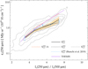 |
Fig. 6. Dependence of the average ϵν(250 μm) versus Iν(250 μm)/Iν(500 μm) on XCO. The shaded area shows the uncertainty due to the CO-to-H2 conversion. Contours and average emissivity as in Fig. 3, model predictions as in Fig. 5. We also show the results of Bianchi et al. (2019) for |

In Fig. 6, we also show the trend obtained using  (dotted line). This recipe, based on global galactic values, has a stronger dependence on metallicity, possibly driven by the relatively smaller number of low-metallicity galaxies in the sample of Hunt et al. (2020); thus, it is probably not suitable for our resolved analysis of relatively higher-metallicity objects. Nevertheless, the trend is not much different from the rest; the exception is that it has lower ϵν(250 μm), since the average conversion factors are larger:
  and
and  , at Iν(250 μm)/Iν(500 μm)=4.5, and 7.5, respectively. The
  recipe has the advantage of resulting in a smaller scatter of ϵν(250 μm) in the highest Iν(250 μm)/Iν(500 μm) bin: it is 22%. However, the scatter produced by the simpler constant
  recipe is even smaller, 15%. Thus, neither
  nor
nor  reduce the scatter with respect to the constant value, as would naively be expected if the adopted formulas were to catch all possible variations of the conversion factor (and dust properties do not change significantly within a galaxy and across galaxies).
5.3.2. Dust-based XCO estimates
If the dust properties, relative to the total gas content, do not vary between galaxies and across environments, it is tempting to use the dust mass or surface density as a tracer of the total ISM (atomic and molecular) budget (Eales et al. 2012; Sandstrom et al. 2013; Jiao et al. 2021). This assumption is used, for example, by Sandstrom et al. (2013), to derive the XCO values and gas-to-dust ratios (and their variations) along the disk of 26 nearby galaxies. Basically, these authors assumed that these quantities do not vary substantially over scales smaller than 1 kpc. On this scale, their solution requires that the total surface density of the gas, obtained by multiplying the dust mass surface density by the gas-to-dust mass ratio, must equal the sum of HI and molecular gas surface densities – with the latter derived from CO observations converted via the XCO factor (and R21). The method obviously relies on the independent determination of the dust mass via a MW dust model (that of Draine & Li 2007). Sandstrom et al. (2013) found XCO values that are slightly lower, but still compatible, with the MW value, with little variation across most of the disks. It is only in galactic centers that XCO is reduced with respect to the disk average. A similar analysis done by Jiao et al. (2021) has offered analogous conclusions.
Our findings apparently suggest that the model dust emissivity is overestimated in denser environments, where the contribution of molecular gas to the total surface density is higher. If this is true, the model-dependent dust (and total gas) content would be underestimated: the lower XCO found by Sandstrom et al. (2013) and Jiao et al. (2021) might potentially be due to this bias. It is true that both papers partially consider variations in the dust properties, by allowing the dust-to-gas mass ratio to vary with respect to the value that is intrinsic to the model grain mixture. However, this approach only scales the amount of dust grains along different sightlines, but does not allow for variations in the emission properties as a function of wavelength. Another problem might arise from the use of the Draine & Li (2007) model, whose emissivity does not match that of the MW cirrus: nevertheless, this global variation can be taken into account in the fitted gas-to-dust mass ratio, while the ϵν(250 μm) versus Iν(250 μm)/Iν(500 μm) trend of the dust model is similar to that of THEMIS (Bianchi et al. 2019).
Since the  recipe adopted in this work is in part derived from the results of Sandstrom et al. (2013), we might also incur the paradox of studying dust emission properties derived from a conversion factor that is itself based on the assumption of a dust model (albeit a different one). Nevertheless, we do not believe that our findings are affected by this choice. In fact, the
  recipe is also based on the dust-independent measurements for
  , and on gas spectral line modeling for denser regions, such as those in ultraluminous IR Galaxies. The reduction of the conversion factor in the inner parts of galaxies was also recently confirmed by Israel (2020), where values as low as
  in galactic central cores were found from the line modeling. Finally, it is to be noted that, apart from the last Iν(250 μm)/Iν(500 μm) bin, the average trend of Fig. 6 is maintained also using the constant
  value.
Matching the emissivity trend to the model predictions indeed requires a smaller XCO, not only in galactic nuclei but over the whole disk. The average emissivity can be aligned to the dust model by using a constant  for all pixels, regardless of metallicity or surface density (red dot-dashed in Fig. 6). Since this conversion factor is significantly different from the values normally accepted for this quantity, it seems reasonable to conclude that the lower than expected ϵν(250 μm) at higher Iν(250 μm)/Iν(500 μm) is not due to an erroneous choice for XCO (or produced by the other biases discussed in this section), – but this is, rather, the result of actual variations in the dust properties and, in particular, of a reduction in the absorption cross-section.
6. Emissivity SED
Using Eq. (1), we also derived the emissivity in the other Herschel bands. The average emissivities and the standard deviation for all wavelengths and Iν(250 μm)/Iν(500 μm) bins are given in Table 2. The same number of pixels is available for each band at each Iν(250 μm)/Iν(500 μm) bin. The only exception is 100 μm, where the data for NGC 2403 and NGC 5194 are not available. Nevertheless, the available pixels in this band are 82% of those available for the rest of the spectral coverage, thus a bias is unlikely. The average SED for each Iν(250 μm)/Iν(500 μm) bin is shown in Fig. 7. As for the average ϵν(250 μm) in Fig. 3, the standard deviation of the mean is smaller than the symbols. For the Iν(250 μm)/Iν(500 μm)=4.5 case we show, as a reference, the total calibration uncertainties for the PACS and SPIRE bands (about 7% and 6%, respectively, using the values quoted by Galliano et al. 2021 and assuming for PACS the same uncertainties for extended sources as for SPIRE).
Average emissivities ϵν and standard deviations, in units of MJy sr−1 (1020 H cm−2)−1, for all wavelengths and Iν(250 μm)/Iν(500 μm) bins.
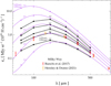 |
Fig. 7. Average emissivity SED for the five Iν(250 μm)/Iν(500 μm) bins of Fig. 3, using |

At Iν(250 μm)/Iν(500 μm)=4.5, the emissivities we estimated for λ ≳ 100 μm are all compatible with the observations in the MW high-latitude cirrus, and with the predictions of the THEMIS diffuse dust model, which are set to fit those observations (see the datapoints and the second purple line from the bottom in Fig. 7). At 70 μm, instead, the emissivity is higher that what predicted by THEMIS: this is expected on the basis of the stronger bias due to ISRF mixing at shorter wavelengths, while the cirrus emission likely results from dust heated by a single radiation field, the LISRF. As discussed in Appendix B, for the wavelength range considered here, ISRF mixing results in a stronger bias when the radiation fields have lower intensities: this is shown by the SED for Iν(250 μm)/Iν(500 μm)=3.5, where our estimates are larger than model predictions up to λ ≲ 160 μm; however, they are still close to the corresponding THEMIS model for λ ≥ 250 μm.
For Iν(250 μm)/Iν(500 μm)> 5, we see the same trends as for ϵν(250 μm) in all the Herschel bands, with the emissivity SED being systematically lower than model predictions (compare the black and purple lines for the same Iν(250 μm)/Iν(500 μm) value in Fig. 7). For λ ≥ 160 μm the THEMIS model could match the average SEDs if scaled by a factor 1/1.4 for the Iν(250 μm)/Iν(500 μm)=5.5 bin and 1/1.9 for the Iν(250 μm)/Iν(500 μm)> 6 bins (i.e., the ratios at 250 μm discussed in Sect. 5). In principle, we could made the THEMIS model reproduce the lower ϵν(250 μm) by lowering its dust-to-gas ratio (0.0074 for the original dust mixture; Jones et al. 2017) by the same factors, while retaining the size distribution and composition (and thus the spectral shape of dust emission). However, this cannot be a plausible explanation: the pixels in the larger Iν(250 μm)/Iν(500 μm) bins have a larger metallicity than in the Iν(250 μm)/Iν(500 μm)=4.5 bin (the “MW reference”), being closer to the galactic centers; thus, their dust-to-gas ratio should be higher, rather than smaller, than for the THEMIS model. Furthermore, for λ < 160 μm, the average emissivity SED has a different spectral shape than models: the ratio Iν(70 μm)/Iν(160 μm), for example, should be higher than in the corresponding model, because of ISRF mixing (or tend to the model, for the more intense ISRFs; see Appendix B); instead, it is lower. The incompatibility of the rescaling factor with the growth of dust-to-gas ratio with metallicity, and the overall difference in spectral shape of the average emissivities with respect to the model, suggests that there could be a variation in the properties of the dust mixture (either in the relative ratios of the various components or in the size distributions, or both).
7. Summary and conclusions
We derived the FIR/submm dust emissivity on a resolved scale (≈400–500 pc) for a sample of nine low-inclination, nearby spiral galaxies. We used maps of the dust emission from the Herschel satellite as well as maps of the atomic and molecular gas column density from the THINGS and HERACLES surveys. Our main findings are as follows:
-
The average ϵν(250 μm) of our sample is compatible with estimates in the MW, for Iν(250 μm)/Iν(500 μm)=4.5 (i.e., the color of dust emission in the MW cirrus). The scatter around this value is limited to 35%, with no evident dependence on local or global galactic properties.
-
For Iν(250 μm)/Iν(500 μm)> 5, the average emissivity is up to a factor ∼2 lower than what is expected based on predictions from models of MW dust. The pixels showing these colors are, on average, closer to the galactic centers and have a higher stellar and gas column density, as well as a higher molecular gas fraction.
-
The results do not depend strongly on the main assumption of the analysis, namely, the choice for the XCO factor; rather, they can be reconciled with the predictions of dust models only using XCO values that are much smaller than what is generally found in the MW and other spirals.
-
The same conclusions are valid for the emissivity ϵν in all Herschel bands with λ ≥ 100 μm.
Our resolved analysis confirms the results obtained by Bianchi et al. (2019), where the disk-averaged ϵν(250 μm) was derived based on a sample of 204 objects. Unless the actual XCO factor used to derive the molecular gas surface density is significantly different from the recipes currently available in the literature, the trends we find for ϵν versus Iν(250 μm)/Iν(500 μm) suggest variations of the dust properties in regions where the radiation field is stronger than the LISFR.
Typically, dust masses in extragalactic objects are derived using grain models based on the MW high latitude cirrus emissivity, which is matched by our extragalactic estimates for Iν(250 μm)/Iν(500 μm)=4.5. As we discuss in Sect. 5, adopting these models to derive the dust masses (or surface densities) for Iν(250 μm)/Iν(500 μm)> 5 could imply an underestimation by up to a factor of two. This uncertainty in the dust mass determination adds to other uncertainties that have been pointed out, such as the comparable discrepancies between dust mass estimates obtained using different dust models (Nersesian et al. 2019; Galliano et al. 2021) and the generally poor knowledge of the emission properties of cosmic dust analogues: for instance, laboratory measurements of the absorption cross sections for amorphous silicates at FIR/submm wavelengths have recently questioned the validity of the optical properties used in current dust models (Demyk et al. 2017) and have been claimed to result in dust mass overestimates by factors ranging from 2 to 20 (Fanciullo et al. 2020).
As a final note, we recall that our analysis assumes homogeneous dust and gas conditions within a few hundred parsecs. While we explored the bias due to a range of starlight intensities, we cannot exclude that the estimated emissivity, even within our spatial scale, could result from dust emission coming from different regions, with different grain properties, gas column densities, and XCO conversion factors. These further biases might affect not only the determination of the emissivity, but also of the dust mass surface density (once the emissivity is assumed from grain models) and XCO determinations (either when the dust mass is used as a proxy for the gas or otherwise); they could be tested numerically with high resolution radiative transfer simulations (as in, e.g., those of Kapoor et al. 2021 and Camps et al. 2022), taking into account the evolution of dust properties with the environment; they could also be checked observationally when higher resolution data for the diffuse continuum emission become available.
The uncertainties given here are larger than those of Bianchi et al. (2019), because we now include the calibration error (and correct an error in the previous estimate of the Iν(250 μm)/Iν(500 μm) uncertainty). While the calibration error is not relevant in the comparison of data obtained with the same instrument at the same wavelength (like the SPIRE determinations of ϵν(250 μm) done in this work and that for the MW in Bianchi et al. 2017), it should be considered when comparing to independent estimates (e.g., the ϵν(250 μm) predictions from THEMIS in Fig. 5) and to estimates at different wavelengths obtained with different instruments and calibration procedures (e.g., ϵν discussed later in Sect. 6).
Acknowledgments
We dedicate this paper to Jonathan Ivor Davies (1955–2021), friend, colleague, and leader of the DustPedia collaboration. We acknowledge support from the INAF mainstream 2018 program “Gas-DustPedia: A definitive view of the ISM in the Local Universe” and from grant PRIN MIUR 2017 – 20173ML3WW_001. We thank E. M. Xilouris for useful comments.
References
- Amorín, R., Muñoz-Tuñón, C., Aguerri, J. A. L., & Planesas, P. 2016, A&A, 588, A23 [NASA ADS] [CrossRef] [EDP Sciences] [Google Scholar]
- Aniano, G., Draine, B. T., Gordon, K. D., & Sandstrom, K. 2011, PASP, 123, 1218 [Google Scholar]
- Aniano, G., Draine, B. T., Hunt, L. K., et al. 2020, ApJ, 889, 150 [NASA ADS] [CrossRef] [Google Scholar]
- Berg, D. A., Pogge, R. W., Skillman, E. D., et al. 2020, ApJ, 893, 96 [NASA ADS] [CrossRef] [Google Scholar]
- Bianchi, S., Giovanardi, C., Smith, M. W. L., et al. 2017, A&A, 597, A130 [NASA ADS] [CrossRef] [EDP Sciences] [Google Scholar]
- Bianchi, S., Casasola, V., Baes, M., et al. 2019, A&A, 631, A102 [NASA ADS] [CrossRef] [EDP Sciences] [Google Scholar]
- Bohlin, R. C., Savage, B. D., & Drake, J. F. 1978, ApJ, 224, 132 [Google Scholar]
- Bolatto, A. D., Wolfire, M., & Leroy, A. K. 2013, ARA&A, 51, 207 [CrossRef] [Google Scholar]
- Boulanger, F., Abergel, A., Bernard, J.-P., et al. 1996, A&A, 312, 256 [NASA ADS] [Google Scholar]
- Camps, P., Kapoor, A. U., Trcka, A., et al. 2022, MNRAS, 512, 2728 [NASA ADS] [CrossRef] [Google Scholar]
- Casasola, V., Cassarà, L. P., Bianchi, S., et al. 2017, A&A, 605, A18 [NASA ADS] [CrossRef] [EDP Sciences] [Google Scholar]
- Casasola, V., Bianchi, S., De Vis, P., et al. 2020, A&A, 633, A100 [NASA ADS] [CrossRef] [EDP Sciences] [Google Scholar]
- Chiang, I.-D., Sandstrom, K. M., Chastenet, J., et al. 2021, ApJ, 907, 29 [NASA ADS] [CrossRef] [Google Scholar]
- Clark, C. J. R., Schofield, S. P., Gomez, H. L., & Davies, J. I. 2016, MNRAS, 459, 1646 [NASA ADS] [CrossRef] [Google Scholar]
- Clark, C. J. R., Verstocken, S., Bianchi, S., et al. 2018, A&A, 609, A37 [NASA ADS] [CrossRef] [EDP Sciences] [Google Scholar]
- Clark, C. J. R., De Vis, P., Baes, M., et al. 2019, MNRAS, 489, 5256 [NASA ADS] [CrossRef] [Google Scholar]
- Compiègne, M., Verstraete, L., Jones, A., et al. 2011, A&A, 525, A103 [Google Scholar]
- Dale, D. A., Helou, G., Contursi, A., Silbermann, N. A., & Kolhatkar, S. 2001, ApJ, 549, 215 [Google Scholar]
- Dale, D. A., Aniano, G., Engelbracht, C. W., et al. 2012, ApJ, 745, 95 [NASA ADS] [CrossRef] [Google Scholar]
- Davies, J. I., Baes, M., Bianchi, S., et al. 2017, PASP, 129 [Google Scholar]
- Demyk, K., Meny, C., Lu, X. H., et al. 2017, A&A, 600, A123 [NASA ADS] [CrossRef] [EDP Sciences] [Google Scholar]
- den Brok, J. S., Chatzigiannakis, D., Bigiel, F., et al. 2021, MNRAS, 504, 3221 [NASA ADS] [CrossRef] [Google Scholar]
- De Vis, P., Dunne, L., Maddox, S., et al. 2017, MNRAS, 464, 4680 [NASA ADS] [CrossRef] [Google Scholar]
- De Vis, P., Jones, A., Viaene, S., et al. 2019, A&A, 623, A5 [NASA ADS] [CrossRef] [EDP Sciences] [Google Scholar]
- Draine, B. T., & Li, A. 2007, ApJ, 657, 810 [CrossRef] [Google Scholar]
- Draine, B. T., Li, A., Hensley, B. S., et al. 2021, ApJ, 917, 3 [CrossRef] [Google Scholar]
- Dwek, E., Arendt, R. G., Fixsen, D. J., et al. 1997, ApJ, 475, 565 [NASA ADS] [CrossRef] [Google Scholar]
- Eales, S., Smith, M. W. L., Auld, R., et al. 2012, ApJ, 761, 168 [NASA ADS] [CrossRef] [Google Scholar]
- Fanciullo, L., Kemper, F., Scicluna, P., Dharmawardena, T. E., & Srinivasan, S. 2020, MNRAS, 499, 4666 [NASA ADS] [CrossRef] [Google Scholar]
- Galliano, F., Nersesian, A., Bianchi, S., et al. 2021, A&A, 649, A18 [EDP Sciences] [Google Scholar]
- Griffin, M. J., Abergel, A., Abreu, A., et al. 2010, A&A, 518, L3 [EDP Sciences] [Google Scholar]
- Groves, B., Krause, O., Sandstrom, K., et al. 2012, MNRAS, 426, 892 [NASA ADS] [CrossRef] [Google Scholar]
- Hensley, B. S., & Draine, B. T. 2021, ApJ, 906, 73 [NASA ADS] [CrossRef] [Google Scholar]
- Hunt, L. K., Draine, B. T., Bianchi, S., et al. 2015, A&A, 576, A33 [NASA ADS] [CrossRef] [EDP Sciences] [Google Scholar]
- Hunt, L. K., De Looze, I., Boquien, M., et al. 2019, A&A, 621, A51 [NASA ADS] [CrossRef] [EDP Sciences] [Google Scholar]
- Hunt, L. K., Tortora, C., Ginolfi, M., & Schneider, R. 2020, A&A, 643, A180 [NASA ADS] [CrossRef] [EDP Sciences] [Google Scholar]
- Israel, F. P. 2020, A&A, 635, A131 [NASA ADS] [CrossRef] [EDP Sciences] [Google Scholar]
- James, A., Dunne, L., Eales, S., & Edmunds, M. G. 2002, MNRAS, 335, 753 [CrossRef] [Google Scholar]
- Jiao, Q., Gao, Y., & Zhao, Y. 2021, MNRAS, 504, 2360 [NASA ADS] [CrossRef] [Google Scholar]
- Jones, A. P., Fanciullo, L., Köhler, M., et al. 2013, A&A, 558, A62 [NASA ADS] [CrossRef] [EDP Sciences] [Google Scholar]
- Jones, A. P., Köhler, M., Ysard, N., Bocchio, M., & Verstraete, L. 2017, A&A, 602, A46 [NASA ADS] [CrossRef] [EDP Sciences] [Google Scholar]
- Kapoor, A. U., Camps, P., Baes, M., et al. 2021, MNRAS, 506, 5703 [NASA ADS] [CrossRef] [Google Scholar]
- Kobulnicky, H. A., & Kewley, L. J. 2004, ApJ, 617, 240 [CrossRef] [Google Scholar]
- Köhler, M., Ysard, N., & Jones, A. P. 2015, A&A, 579, A15 [NASA ADS] [CrossRef] [EDP Sciences] [Google Scholar]
- Leroy, A. K., Walter, F., Bigiel, F., et al. 2009, AJ, 137, 4670 [Google Scholar]
- Leroy, A. K., Walter, F., Sandstrom, K., et al. 2013, AJ, 146, 19 [Google Scholar]
- Leroy, A. K., Rosolowsky, E., Usero, A., et al. 2022, ApJ, 927, 149 [NASA ADS] [CrossRef] [Google Scholar]
- Low, F. J., Young, E., Beintema, D. A., et al. 1984, ApJ, 278, L19 [Google Scholar]
- Madden, S. C., Cormier, D., Hony, S., et al. 2020, A&A, 643, A141 [NASA ADS] [CrossRef] [EDP Sciences] [Google Scholar]
- Mathis, J. S., Mezger, P. G., & Panagia, N. 1983, A&A, 128, 212 [NASA ADS] [Google Scholar]
- Morrissey, P., Conrow, T., Barlow, T. A., et al. 2007, ApJS, 173, 682 [Google Scholar]
- Mosenkov, A. V., Sotnikova, N. Y., & Reshetnikov, V. P. 2014, MNRAS, 441, 1066 [Google Scholar]
- Mosenkov, A. V., Baes, M., Bianchi, S., et al. 2019, A&A, 622, A132 [NASA ADS] [CrossRef] [EDP Sciences] [Google Scholar]
- Nersesian, A., Xilouris, E. M., Bianchi, S., et al. 2019, A&A, 624, A80 [NASA ADS] [CrossRef] [EDP Sciences] [Google Scholar]
- Osterbrock, D. E. 1989, Astrophysics of Gaseous Nebulae and Active Galactic Nuclei (University Science Books) [Google Scholar]
- Pettini, M., & Pagel, B. E. J. 2004, MNRAS, 348, L59 [NASA ADS] [CrossRef] [Google Scholar]
- Pilbratt, G. L., Riedinger, J. R., Passvogel, T., et al. 2010, A&A, 518, L1 [NASA ADS] [CrossRef] [EDP Sciences] [Google Scholar]
- Pilyugin, L. S., & Grebel, E. K. 2016, MNRAS, 457, 3678 [NASA ADS] [CrossRef] [Google Scholar]
- Pilyugin, L. S., & Mattsson, L. 2011, MNRAS, 412, 1145 [NASA ADS] [Google Scholar]
- Pilyugin, L. S., Grebel, E. K., & Mattsson, L. 2012, MNRAS, 424, 2316 [NASA ADS] [CrossRef] [Google Scholar]
- Pilyugin, L. S., Grebel, E. K., & Kniazev, A. Y. 2014, AJ, 147, 131 [NASA ADS] [CrossRef] [Google Scholar]
- Planck Collaboration Int. XVII. 2014, A&A, 566, A55 [NASA ADS] [CrossRef] [EDP Sciences] [Google Scholar]
- Poglitsch, A., Waelkens, C., Geis, N., et al. 2010, A&A, 518, L2 [NASA ADS] [CrossRef] [EDP Sciences] [Google Scholar]
- Priestley, F. D., & Whitworth, A. P. 2020, MNRAS, 494, L48 [NASA ADS] [CrossRef] [Google Scholar]
- Sandstrom, K. M., Leroy, A. K., Walter, F., et al. 2013, ApJ, 777, 5 [Google Scholar]
- Walter, F., Brinks, E., de Blok, W. J. G., et al. 2008, AJ, 136, 2563 [Google Scholar]
- Werner, M. W., Roellig, T. L., Low, F. J., et al. 2004, ApJS, 154, 1 [NASA ADS] [CrossRef] [Google Scholar]
- Ysard, N., Juvela, M., Demyk, K., et al. 2012, A&A, 542, A21 [NASA ADS] [CrossRef] [EDP Sciences] [Google Scholar]
- Zubko, V., Dwek, E., & Arendt, R. G. 2004, ApJS, 152, 211 [NASA ADS] [CrossRef] [Google Scholar]
- Zurita, A., Florido, E., Bresolin, F., Pérez-Montero, E., & Pérez, I. 2021, MNRAS, 500, 2359 [Google Scholar]
Appendix A: Metallicity gradients
The most reliable determination of gas metallicity is through the so-called direct method, namely, by measuring the physical parameters of the gas: the electron temperature from the ratio of a weak auroral line (e.g., [OIII] 4363 Å) and a strong emission line from the same ionic species (e.g., [OIII] 5007 Å); the electron density, from the ratio of two lines of the same ionic species very close in λ (e.g., [SII] 6717, 6731 Å ; see, e.g., Osterbrock 1989). From strong lines (e.g., [OIII] and [OII] for O/H) and hydrogen recombination lines, solving the equation of the statistical equilibrium equations at the provided conditions of temperature and density, we can derive the ionic abundances. The metallicity is then obtained summing up the ionic abundances, eventually correcting for the ionic abundances of the unseen ionization stages. After estimating the metallicity in various H II regions along the disk of a galaxy, a metallicity gradient can be determined. Unfortunately, only a few galaxies have gradients obtained with the direct method: in the recent compilation and analysis by Zurita et al. (2021), O/H gradients are provided for 12 galaxies only, only 4 of which are in our sample. Instead, gradients for all our targets are available from Pilyugin et al. (2014). They have been derived from measurements of strong lines only, adopting empirical methods that perform well when compared to gradients obtained with the direct method (Pilyugin & Mattsson 2011; Pilyugin et al. 2012).
From an extensive compilation of literature and archival line emission measurements, De Vis et al. (2019) derived metallicities for a large fraction of DustPedia galaxies. These authors used a variety of strong-line calibration methods and provided characteristic metallicities (at 0.4 × R25) and metallicity gradients (adopting average gradients as priors for galaxies with few measurements across the disk). It is a well known fact that the estimate of the gradient depends on the adopted metallicity calibrator (see, e.g., Zurita et al. 2021). For one of our targets, NGC 5194, the gradient from direct measurements (Berg et al. 2020; Zurita et al. 2021) as well as from the strong-line calibration of Pilyugin et al. (2014) is negative, as usually found in many galaxies. Instead, the metallicity distribution is flat using the PG16S calibration (Pilyugin & Grebel 2016), the preferred choice of De Vis et al. (2019). For the N2 method (Pettini & Pagel 2004), which was chosen by Bianchi et al. (2019), the gradient found by De Vis et al. (2019) for NGC 5194 becomes positive (as also shown by Zurita et al. 2021).
For the DustPedia galaxies in common between the two samples, we compared the characteristic metallicities and gradients obtained by De Vis et al. (2019) with those from Pilyugin et al. (2014). When using the N2 or PG16S calibrations, the characteristic metallicities from De Vis et al. (2019) are within 0.05 dex of those from Pilyugin et al. (2014). The smallest difference and scatter in the gradients, instead, is for the KK04 theoretical calibration of Kobulnicky & Kewley (2004, see Fig. A.1, red datapoints). The metallicities obtained with this methods have higher values, but once they are corrected by 0.45 dex, they show a small scatter with respect to those from Pilyugin et al. (2014). A similar comparison is shown in Fig. A.1 with Zurita et al. (2021), however, for a smaller number of objects (blue and grey datapoints).
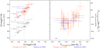 |
Fig. A.1. Comparison between the characteristic metallicities (at 0.4 × R25; left) and metallicity gradients (right) obtained by De Vis et al. (2019) for DustPedia galaxies with the Kobulnicky & Kewley (2004) calibration (on ordinates), and the same values from Pilyugin et al. (2014) and Zurita et al. (2021, on abscissae; red and blue datapoints, respectively). For each galaxy, characteristic metallicities and gradients on abscissae have been derived from the original data using the same value for R25 (from De Vis et al. 2019). Grey and black datapoints on the left panel show the comparison with Pilyugin et al. (2014) and Zurita et al. (2021), respectively, once the characteristic metallicity of De Vis et al. (2019) has been corrected by 0.45 dex. De Vis et al. (2019) have 58 galaxies in common with Pilyugin et al. (2014) (9 with Zurita et al. 2021). Datapoints for the galaxies used in this work are shown with a circle. |
In this work we used the metallicity gradients from Pilyugin et al. (2014): this is the more straightforward choice, because of the "regular" gradient for NGC 5194 and because there is no need for corrections as for the KK04 metallicities of De Vis et al. (2019). Furthermore, this choice resulted in a slightly smaller scatter of ϵν(250 μm). Nevertheless, the exact choice of the metallicity gradient appears to have little impact on the results of this work, as shown by the small differences in the average emissivities in Fig. A.2.
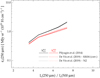 |
Fig. A.2. Average ϵν(250 μm) versus Iν(250 μm)/Iν(500 μm) for different choices of XCO and metallicity gradients. |
Appendix B: Effects of ISRF mixing
The emissivity is a useful benchmark for models if dust emission comes from grains heated by a uniform ISRF. If instead observations include emission from grains exposed to a distribution of starlight intensities, the spectral shape of the emissivity might be affected by the range in ISRFs; it is then more difficult to extract from the SED the signatures of grain optical properties and size distributions. We explore here the effects of the mixing of ISRF intensities on the FIR-to-submm emissivities, using the THEMIS model and the DustEM code (Compiègne et al. 2011) to predict dust emission under different heating conditions.
The reference model used in the main text consists of the simple case of the THEMIS dust mixture heated by a uniform ISRF. Usually, the radiation field heating the dust is scaled on the local one, the LISRF of Mathis et al. (1983), by setting ISRF = U × LISRF. In Fig. B.1 (left panel), we show ϵν(250 μm) versus Iν(250 μm)/Iν(500 μm) for values of the scale factor ranging from U = 0.1 to 20. As U grows the ISRF becomes more intense, and both ϵν(250 μm) and Iν(250 μm)/Iν(500 μm) increase. In Fig. B.1 (right panel) we show the emissivity SEDs for the five Iν(250 μm)/Iν(500 μm) bins used in the analysis: from the lower to the upper, SEDs have Iν(250 μm)/Iν(500 μm)=3.5, 4.5, 5.5, 6.5, and 7.5, corresponding to U = 0.35, 1, 2.8, 8.2, and 26.
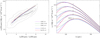 |
Fig. B.1. Variations of ϵν for the THEMIS model under various heating conditions. Left panel: ϵν(250 μm) versus Iν(250 μm)/Iν(500 μm) for radiation fields scaled on the LISRF, with different values for γ, the fraction of dust heated by a radiation field distribution (α = 2 and Umax = 107 for γ ≠ 0; Eq. B.1); and for ISRFs dominated by UV (young stars) or red (old stars) radiation (γ = 0; see text for details). Contour plots (gray lines) and averages (black line) from the analysis in the main text are shown for reference (Fig. 3). Right panel: ϵν versus λ for the central values of the Iν(250 μm)/Iν(500 μm) bins and the same cases as in the left panel. Dots represent the emissivities integrated over the Herschel filter response functions (for the LISRF, γ = 0 case only). |
Draine & Li (2007) introduced the consuetude of describing the SED of galaxies as the sum of a dust component heated by a radiation field of intensity Umin and another, hotter, component heated by a power-law distribution with Umin < U < Umax (as proposed by Dale et al. 2001). It is
 (B.1)
(B.1)
where γ is the fraction of dust heated by the ISRF powerlaw distribution and α its spectral index (Eq. B.1 being formally correct for α > 1). When fitting global SEDs, Md is the total dust mass; for resolved analyses, it is the dust mass within the resolution area. Typically, α ≈ 2 both in fits of global (Dale et al. 2012) and resolved SEDs (Aniano et al. 2020). We follow Aniano et al. (2020) and use Umax = 107, although for α = 2 and the wavelengths of interest here there is little difference if Umax is set as low as 104.
The case of a uniform ISRF is equivalent to adopting γ = 0 in Eq. B.1. When global SEDs are analyzed, γ is found to be a few percent and the dust heating (and emission) is still dominated by the Umin component (Dale et al. 2012). The composite emissivity derived with γ = 0.05 is shown in Fig. B.1. The ϵν(250 μm) versus Iν(250 μm)/Iν(500 μm) trend is almost unaltered with respect to the reference γ = 0 case, although the average radiation field corresponding to each Iν(250 μm)/Iν(500 μm) bin becomes larger, ⟨U⟩=0.53, 1.5, 4.1, 12, and 36 (see the aforementioned references for the mathematical definition of ⟨U⟩). Emissivity values for λ ≥ 160 μm are within less than 2% of those for a uniform ISRF, while values at the shorter Herschel wavelengths could be much larger, though the difference reduces for the more intense ISRFs (and larger emissivities).
The contribution of the power-law distribution, instead, is found to be larger in resolved studies: for the galaxies in common with our sample, and at a comparable resolution to the one adopted here, it is ⟨γ⟩≈0.3 in the work of Aniano et al. (2020). Again, the ϵν(250 μm) versus Iν(250 μm)/Iν(500 μm) trend changes little, although the reference Iν(250 μm)/Iν(500 μm) values are now produced by ⟨U⟩=1.1, 3.3, 9, 26, and 79. The difference with the uniform ISRF heating is now larger: the emissivity in the three SPIRE bands is ≈10% smaller for Iν(250 μm)/Iν(500 μm)=3.5 and 7% for 4.5, reducing to less than 5% for larger Iν(250 μm)/Iν(500μm); at shorter wavelengths, instead, the emissivity is larger (a factor 2 at 100 μm for Iν(250 μm)/Iν(500 μm)=3.5). For a given Iν(250 μm)/Iν(500 μm), the general effect of the mixing of radiation fields is then that of a broadening of the SED, with relatively small changes in the submm emissivity, but larger changes for λ ≲ 160 μm and a shift of the peak emission towards smaller wavelengths.
The basic assumption in the formalism we use here is that the spectral shape of the ISRF does not change, as it is always the same as that of the LISFR. Draine et al. (2021) investigated the effects of different spectra and found that emission in the mid-infrared can change significantly if the ISRF is richer in UV radiation. However, at the wavelengths of interest here, the spectral shape of the radiation field has smaller effects: this is shown in Fig. B.1, where we plot the cases for the two extreme spectra in the work of Draine et al. (2021), a UV-rich 3 Myr old starburst, and a UV-poor, red, spectrum from a very old stellar population (used by Groves et al. 2012 to describe the bulge population of M 31). Changes in the emissivity (which are stronger for the UV-rich heating radiation field) are still within those we have considered so far, in particular for the larger Iν(250 μm)/Iν(500 μm) where observations diverge from our reference model. We do not consider this case any further, and revert to the standard scaling on the LISRF.
An alternative ISRF distribution is used by Galliano et al. (2021), neglecting the δ(U − Umin) component of Eq. B.1 (or, equivalently, setting γ = 1). The shape of the dust SED illuminated by this distribution can then vary as a result of changes in Umin, α, and in the U range, via the parameter ΔU = Umax − Umin. By fitting the global SEDs of 798 DustPedia galaxies, Galliano et al. (2021) find median values α ≈ 2.1 and ΔU ≈ 240. The emissivities for this case are shown in Fig. B.2. In the SPIRE bands, ϵν is biased low by ≈15% and 10% for Iν(250 μm)/Iν(500 μm)=3.5 and 4.5, respectively, while the Iν(250 μm)/Iν(500 μm) bins now corresponds to ISRF intensities ⟨U⟩=0.5, 1.5, 4.1, 11 and 32. Again, the trends we obtain for this model are not too different from those of the reference one and do not reproduce the observed averages at larger Iν(250 μm)/Iν(500 μm) values. While waiting for an analysis of resolved SEDs using the Galliano et al. (2021) formalism, we cannot exclude the presence of broader ISRF distributions in localized regions of a galaxy. In particular, by choosing α < 2 and appropriate ΔU values, we can have ϵν(250 μm) versus Iν(250 μm)/Iν(500 μm) values approaching the observations: we show in the left panel of Fig. B.2 two cases with ΔU = 104, one for α = 1.5, passing close to the observed average at Iν(250 μm)/Iν(500 μm)=5.5 and one for α = 1.3, near the Iν(250 μm)/Iν(500 μm)=7.5 value (for a given α, the low-ϵν(250 μm) part of the trend shifts to the right as ΔU increases). Despite matching ϵν(250 μm), however, these two cases cannot reproduce the emissivity SED, since they have emission peaks at wavelengths much shorter than what we find (Fig. B.2, right panel).
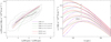 |
Fig. B.2. Same as Fig. B.1, but for different radiation mixes. Beside the reference γ = 0 case, we show results for γ = 1 and various values for α and ΔU; and for models taking into account the biases described by Priestley & Whitworth (2020), assuming that grains exposed to the attenuated radiation field have the THEMIS properties (case 1) or those of the CMM grain mixture (case 2; see text for details). For clarity, in the left panel the α = 1.5 SED is shown for Iν(250 μm)/Iν(500 μm)=5.5 only, and the α = 1.3 SED for Iν(250 μm)/Iν(500 μm)=7.5 only. |
The power-law distribution in Eq. B.1 was proposed by Dale et al. (2001) as a way to describe different heating conditions, with α ranging from 2.5 for a diffuse, uniform medium where the ISRF intensity decreases mainly with the increase of the distance between dust and the sources and up to α = 1 for dense clouds where the ISRF intensity reduces because of dust absorption. While a proper radiative transfer model is needed to investigate the changes in the heating fields due to dust attenuation (see, e.g., Ysard et al. 2012 for the variations in the dust emissivity of externally illuminated clouds of size up to a few parsecs), a simpler scenario has been proposed by Priestley & Whitworth (2020): they suggest that, along lines of sight of high ISM column density, a considerable fraction of the dust emission comes from grains heated to colder temperatures by a radiation field attenuated by dust itself. Using their formalism, we explored the case for column density ΣISM=100 M⊙ pc−2, corresponding to a dust optical depth in the V-band τV ≈ 6 for the average MW properties (Bohlin et al. 1978). We adopted the rather extreme case in which 25% of the dust emission is due to dust heated by an unattenuated ISRF of intensity U, and 75% to dust heated by an attenuated radiation field which, assuming the MW extinction law and that all emission is behind a screen with τV = 6, has a reduced global intensity corresponding to about 0.15 × U (though with a redder spectral shape with respect to the LISRF). We show in Figure B.2, the results using the THEMIS model for dust exposed to the unattenuated field, and two different properties for dust at higher density: in the first case, we again use THEMIS; in the second case, we use the CMM model of Köhler et al. (2015), which takes into account dust growth and coagulation in denser media. When using the THEMIS model for the higher density environment, the estimate of the emissivity is ≈20% lower in the SPIRE bands for Iν(250 μm)/Iν(500 μm)=4.5; for CMM dust, the mixing of heating fields conjures with the higher grain cross sections, and the difference is smaller (ϵν is higher by 15%). In any case, the trend of ϵν(250 μm) versus Iν(250 μm)/Iν(500 μm) is not significantly altered from that of the single U case; the bias for λ ≥ 160 μm and Iν(250 μm)/Iν(500 μm)> 5 is ≈15% at maximum. Köhler et al. (2015) also present other dust aggregate models which, however, result in higher emissivities with respect to CMM (and THEMIS; see also Bianchi et al. 2019) and thus cannot be reconciled with the observed mean ϵν(250 μm) at Iν(250 μm)/Iν(500 μm)=4.5 and the trend for Iν(250 μm)/Iν(500 μm)> 5.
In conclusion, the mixing of ISRF intensities is not likely to bias strongly the estimate of ϵν for λ ≥ 160 μm, at least for Iν(250 μm)/Iν(500 μm)> 5. It would have been possible to use ϵν(160 μm) as a reference value, as it shows the lower bias, ≤6% in most test cases shown here. We prefer nevertheless ϵν(250 μm) since it is a common reference in the literature, and it has been used for the global emissivity estimates of Bianchi et al. (2019) and derived directly in the foreground of the Virgo Cluster from SPIRE observations of the MW cirrus (which was undetected in PACS images; Bianchi et al. 2017).
All Tables
Average emissivities ϵν and standard deviations, in units of MJy sr−1 (1020 H cm−2)−1, for all wavelengths and Iν(250 μm)/Iν(500 μm) bins.
All Figures
|
Fig. 1. Dataset and results for NGC 5457. The top row shows the 250 μm image, the molecular gas column density derived from CO observations for |
| In the text | |
|
Fig. 2. Maps of ϵν(250 μm) for the rest of the sample (assuming |
| In the text | |
|
Fig. 3. Emissivity at 250 μm, ϵν(250 μm) versus the Iν(250 μm)/Iν(500 μm) ratio (assuming |
| In the text | |
|
Fig. 4. ϵν(250 μm) versus Iν(250 μm)/Iν(500 μm), same grey contours as in Fig. 3. In each panel, the color map shows the average value of the following quantities: Σ⋆, SNUV/S3.6 μm, fmol and ΣISM. |
| In the text | |
|
Fig. 5. ϵν(250 μm) versus Iν(250 μm)/Iν(500 μm). Comparison between our results and the MW value for the cirrus. We also show the behavior of the THEMIS dust model under ISRFs of growing intensities (dots are for U = 0.2, 0.5, 1, 2, 5, 10, 20, and 50 from left to right, with ISRF = U × LISRF; see Appendix B). Grey contours and average emissivity as in Fig. 3. The errorbars for the average emissivity show the impact on ϵν(250 μm) of the SPIRE calibration error. |
| In the text | |
|
Fig. 6. Dependence of the average ϵν(250 μm) versus Iν(250 μm)/Iν(500 μm) on XCO. The shaded area shows the uncertainty due to the CO-to-H2 conversion. Contours and average emissivity as in Fig. 3, model predictions as in Fig. 5. We also show the results of Bianchi et al. (2019) for |
| In the text | |
|
Fig. 7. Average emissivity SED for the five Iν(250 μm)/Iν(500 μm) bins of Fig. 3, using |
| In the text | |
|
Fig. A.1. Comparison between the characteristic metallicities (at 0.4 × R25; left) and metallicity gradients (right) obtained by De Vis et al. (2019) for DustPedia galaxies with the Kobulnicky & Kewley (2004) calibration (on ordinates), and the same values from Pilyugin et al. (2014) and Zurita et al. (2021, on abscissae; red and blue datapoints, respectively). For each galaxy, characteristic metallicities and gradients on abscissae have been derived from the original data using the same value for R25 (from De Vis et al. 2019). Grey and black datapoints on the left panel show the comparison with Pilyugin et al. (2014) and Zurita et al. (2021), respectively, once the characteristic metallicity of De Vis et al. (2019) has been corrected by 0.45 dex. De Vis et al. (2019) have 58 galaxies in common with Pilyugin et al. (2014) (9 with Zurita et al. 2021). Datapoints for the galaxies used in this work are shown with a circle. |
| In the text | |
|
Fig. A.2. Average ϵν(250 μm) versus Iν(250 μm)/Iν(500 μm) for different choices of XCO and metallicity gradients. |
| In the text | |
|
Fig. B.1. Variations of ϵν for the THEMIS model under various heating conditions. Left panel: ϵν(250 μm) versus Iν(250 μm)/Iν(500 μm) for radiation fields scaled on the LISRF, with different values for γ, the fraction of dust heated by a radiation field distribution (α = 2 and Umax = 107 for γ ≠ 0; Eq. B.1); and for ISRFs dominated by UV (young stars) or red (old stars) radiation (γ = 0; see text for details). Contour plots (gray lines) and averages (black line) from the analysis in the main text are shown for reference (Fig. 3). Right panel: ϵν versus λ for the central values of the Iν(250 μm)/Iν(500 μm) bins and the same cases as in the left panel. Dots represent the emissivities integrated over the Herschel filter response functions (for the LISRF, γ = 0 case only). |
| In the text | |
|
Fig. B.2. Same as Fig. B.1, but for different radiation mixes. Beside the reference γ = 0 case, we show results for γ = 1 and various values for α and ΔU; and for models taking into account the biases described by Priestley & Whitworth (2020), assuming that grains exposed to the attenuated radiation field have the THEMIS properties (case 1) or those of the CMM grain mixture (case 2; see text for details). For clarity, in the left panel the α = 1.5 SED is shown for Iν(250 μm)/Iν(500 μm)=5.5 only, and the α = 1.3 SED for Iν(250 μm)/Iν(500 μm)=7.5 only. |
| In the text | |
Current usage metrics show cumulative count of Article Views (full-text article views including HTML views, PDF and ePub downloads, according to the available data) and Abstracts Views on Vision4Press platform.
Data correspond to usage on the plateform after 2015. The current usage metrics is available 48-96 hours after online publication and is updated daily on week days.
Initial download of the metrics may take a while.