| Issue |
A&A
Volume 664, August 2022
|
|
|---|---|---|
| Article Number | A11 | |
| Number of page(s) | 13 | |
| Section | Interstellar and circumstellar matter | |
| DOI | https://doi.org/10.1051/0004-6361/202243566 | |
| Published online | 04 August 2022 | |
NIR spectroscopic survey of protostellar jets in the star-forming region IC 1396N★,★★
1
INAF – Osservatorio Astrofisico di Arcetri,
Largo E. Fermi 5,
50125
Firenze, Italy
e-mail: This email address is being protected from spambots. You need JavaScript enabled to view it.
2
Departament de Física Quàntica i Astrofísica, Institut de Ciències del Cosmos, Universitat de Barcelona, IEEC-UB,
Martí i Franquès, 1,
08028
Barcelona, Spain
3
Institut de Ciències de l’Espai (ICE), CSIC,
Carrer de Can Magrans, s/n,
08193
Cerdanyola del Vallès, Catalonia, Spain
4
Institut d’Estudis Espacials de Catalunya (IEEC),
08034
Barcelona, Catalonia, Spain
Received:
16
March
2022
Accepted:
5
May
2022
Abstract
Context. The bright-rimmed cloud IC 1396N, associated with an intermediate-mass star-forming region, hosts a number of CO, molecular hydrogen, and Herbig-Haro (HHs) outflows powered by a set of millimetre compact sources.
Aims. The aim of this work is to characterise the kinematics and physical conditions of the H2 emission features spread throughout the IC 1396N region. The features appear as chains of knots with a jet-like morphology and trace different H2 outflows. We also obtain further information about (and an identification of) the driving sources.
Methods. Low-resolution, long-slit near-infrared spectra were acquired with the NICS camera at the TNG telescope, using grisms KB (R ~ 1200), HK, and JH (R ~ 500). Several slit pointings and position angles were used throughout the IC 1396N region in order to sample a number of the H2 knots that were previously detected in deep H2 2.12 μm images.
Results. The knots exhibit rich ro–vibrational spectra of H2, consistent with shock-excited excitation, from which radial velocities and relevant physical conditions of the IC 1396N H2 outflows were derived. These also allowed estimating extinction ranges towards several features. [Fe ii] emission was only detected towards a few knots that also display unusually high H2 1–0 S(3)/S(1) flux ratios. The obtained radial velocities confirm that most of the outflows are close to the plane of the sky. Nearby knots in the same chain often display different radial velocities, both blue–shifted and red–shifted, which we interpret as due to ubiquitous jet precession in the driving sources or the development of oblique shocks. One of the chains (strand A, i.e. knots A1 to A15) appears as a set of features trailing a leading bow-shock structure consistent with the results of 3D magneto-hydrodynamical models. The sides of the leading bow shock (A15) exhibit different radial velocities. We discuss possible explanations. Our data cannot confirm whether strands A and B have both originated in the intermediate mass young stellar object [BGE2002] BIMA 2 because a simple model of a precessing jet cannot account for their locations.
Conclusions. Near-infrared spectroscopy has confirmed that most of the H2 ro-vibrational emission in IC 1396N is shock-excited rather than uv-excited in photon-dominated regions. It has shown a complex kinematical structure in most strands of emitting knots as well.
Key words: ISM: jets and outflows / ISM: individual objects: IC1396N / stars: formation / infrared: ISM / techniques: spectroscopic
Tables 3–5 are only available at the CDS via anonymous ftp to cdsarc.u-strasbg.fr (130.79.128.5) or via http://cdsarc.u-strasbg.fr/viz-bin/cat/J/A+A/664/A11
Based on observations made with the Italian Telescopio Nazionale Galileo (TNG) operated on the island of La Palma by the Fundación Galileo Galilei of the INAF (Istituto Nazionale di Astrofisica) at the Spanish Observatorio del Roque de los Muchachos of the Instituto de Astrofisica de Canarias (time awarded by IAC, programme CAT_32/2007, P. I. M. Beltrán).
© F. Massi et al. 2022
 Open Access article, published by EDP Sciences, under the terms of the Creative Commons Attribution License (https://creativecommons.org/licenses/by/4.0), which permits unrestricted use, distribution, and reproduction in any medium, provided the original work is properly cited.
This article is published in open access under the Subscribe-to-Open model. This email address is being protected from spambots. You need JavaScript enabled to view it. to support open access publication.
1 Introduction
The bright-rimmed cloud IC 1396N (also known as BRC38; Sugitani et al.1991), associated with the H ii region IC 1396, is an interesting laboratory for studying a range of star formation processes in progress. It exhibits a cometary structure, whose bright rim faces the ionising star HD 206267 towards the south, and its tail points to the north. HD 206267 is a multiple system with HD 206267 Aa (O5V+B0V) and Ab (O9V), and is located in the cluster Trumpler 37 (Maíz Apellániz &Barbá2020) inside the H ii region IC1396. The distance to the system estimated from Gaia parallaxes is  pc (Maíz Apellániz &Barbá 2020). This value points to a slightly larger distance to IC 1396N than assumed in previous works (usually 750 pc). This is also confirmed by other authors using Gaia data. Thus, we adopt here a revised distance of 910 ± 49 pc from the catalogue of distances to molecular clouds of Zucker et al.(2020), obtained by combining stellar photometric data and Gaia parallaxes. Stellar optical polarisation measurements show that the magnetic field in the cloud is almost aligned with the ionising radiation, forming an average angle of ~20° with it (Soam et al.2018). The magnetic field is in fact roughly parallel to the Galactic plane, as expected on a larger scale.
The head of the cloud is characterised by diffuse emission in the mid-infrared (MIR; see e.g. Fig. 5 of Beltrán et al.2009), whereas the tail appears as a dark lane running from south to north (see e.g. the JHK image in Fig. 1 of Beltrán et al. 2009). This morphology is well reflected in millimetre (mm) line emission (Codella et al.2001; Sugitani et al.2002). The star formation activity inside the cloud is clearly evident because both HH objects are visible at optical wavelengths (Reipurth et al.2003) and chains of knots of H2 2.12 μm line emission are detected in the near-infrared (NIR; Nisini et al.2001; Sugitani et al.2002; Caratti o Garatti et al.2006; Beltrán et al.2009). Most of the H2 knots originated in shocked gas in the outflows rather than in uv-excited fluorescence, as confirmed by their coincidence with mm outflows (Codella et al. 2001; Beltrán et al. 2002, Beltrán et al. 2012). The stellar population around the head was studied in the NIR, MIR, and in X-rays to discusspossible scenarios of triggered star formation (Getman et al. 2007; Beltrán et al.2009;Choudhury et al. 2010).
The H2 knots towards the head of IC 1396N are associated with the intermediate-mass young stellar object (YSO) IRAS 21391+5802 (and other nearby YSOs; Beltrán et al.2002). Other H2 knots and the Herbig-Haro object HH 777 in the middle of the cloud are associated with the NIR source HH 777/IRS331 (Reipurth et al.2003; Beltrán et al.2002), whereas most of the H2 knots in the tail of the cloud are associated with two mm compact sources (Codella et al.2001; Beltrán et al.2012). In particular, Beltrán et al. (2012) discussed what was probably the first documented occurrence of the interaction between outflows, causing a complex structure of H2 line emission. So far, only one other case of a possible outflow collision has been reported (in BHR 71; see Zapata et al. 2018).
The ro-vibrational line v = 1–0 S(1) at 2.12 μm of molecular hydrogen has proven to be an efficient tracer of protostellar jets and outflows through narrow-band imaging. H2 ro-vibrational emission spectra originate in slow, non-dissociative C-shocks or in the post-shock regions of fast (≳25–50 KM S–1) dissociative J-shocks (e.g. Hollenbach & McKee1979, Hollenbach & McKee 1980, Hollenbach & McKee 1989; Kaufman & Neufeld1996). H2 line emission also occurs in photon-dominated regions (PDRs) due to fluorescent excitation (Black & van Dishoeck1987). In principle, radiative fluorescent emission can be distinguished from thermal emission based on the ro-vibrational spectra if gas densities are ≲104 cm–3, whereas thermal emission becomes dominant at higher gas densities even with intense UV fields (Sternberg & Dalgarno 1989). In this respect, higher-excitation ro-vibrational lines falling in the J and Hbands can be instrumental in distinguishing the excitation mechanism (Black & van Dishoeck1987), which unfortunately happens to be a spectral region that is more extincted than K. Other interesting lines may occur in the JH band, such as the [Fe ii] lines originating from the upper level 3d6(5D)4s a4D7/2of ionised iron at 1.6440, 1.3209, and 1.2570 μm, which trace J-shocks (Hollenbach & McKee 1989). When these are present, they can be used to estimate extinction (Pecchioli et al. 2016).
With this in mind, we carried out a long-slit low-resolution (R ~ 500 to 1250) survey of IC 1396N in the JHK bands to distinguish the different flows (and to distinguish between shock-excited and fluorescent-excited H2 emission) in the head of the cloud and identify new possible driving sources. Caratti o Garatti et al.(2006) have reported on long-slit low-resolution (R ~ 500) NIR spectra of targets in IC 1396N, but they are limited to the two chains (or strands) of knots called A and B towards the head of the cloud without information about the single knots of each chain.
The paper is laid out as follows: the observations and data reduction are described in Sect. 2, the main results are described in Sect. 3 and are further discussed in Sect.4. Section 5 summarises the main findings, and some important issues are detailed in the appendix.
2 Observations and Data Reduction
Low-resolution long-slit spectra were obtained at several slit positions (see Fig. 1) with the NIR camera NICS (Baffa et al. 2001) at the 3.58 m Telescopio Nazionale Galileo (TNG) on August 22, 23, and 24, 2007, using grisms KB (spanning the spectral range 1.95–2.34 μm), HK (1.40–2.50 μm), and JH (1.15– 1.75 μm), and a 1″ wide slit, achieving spectral resolutions of 1250, 500, and 500, respectively. The plate scale is 0.25″pix–1, yielding a field of view (fov) of 4′2 × 4′2, whereas the slit length is 4′. For each integration, pointing and slit position angle (PA) were selected so that several knots were encompassed by the slit at the same time (see Fig. 1). The slit was positioned on the plane of the sky by using reference stars. PA and reference stars were chosen based on a careful analysis of the H2 2.12 μm image of Beltrán et al. (2009). All observations were carried out as multiple AB cycles, taking two exposures with the target shifted along the slit (i.e. in positions A and B). However, as several knots span the slit length in various positions, the slit was moved completely off-source in the B position. Spectra of two telluric standards, an A0 star (HIP 109079) and a G2V star (HIP 110327), were obtained with one ABBA cycle each per grism at the beginning, in the middle, and at the end of each night, with the slit roughly oriented at the parallactic angle. On July 24, HIP 109079 was imaged in various positions along the slit to allow deriving a set of traces in different parts of the frame to use as references in the subsequent extraction of the target spectra. Details are given in Table 1. Halogen and Ar lamp spectra were obtained in the afternoon preceding each observing night for flat-fielding and wavelength calibrating.
The spectra were reduced using standard IRAF routines1. For each night run, the halogen lamp frames taken in the afternoon were averaged together and normalised row by row to a third-degree polynomial fit, as advised in the TNG web-page. The science frames were corrected for flat field and for cross-talk using the software provided by the TNG staff, and bad pixels were removed. For each AB cycle, the second frame was then subtracted from the first frame. The 2D spectra were then straightened and wavelength calibrated using the lines in the afternoon Ar lamp spectra. When the same target was acquired with more than one AB cycle, we checked that the spatial profiles in a bright emission line were consistent with each other. The subtracted 2D frames were then added together (generally, no shift was needed in the spatial direction to overlap the spectra). In a few cases only did we find some inconsistencies, and we did not combine the frames. These were clearly caused by small pointing differences.
There is usually some residual shift (a few Å to a few dozen Å) along the wavelength axis between the Ar lamp frames and the target frames. This shift is variable with pointing location and slit position angle (see Massi et al.2008). We therefore realigned the science and telluric standard frames taken during the same night by using sky emission lines as references. Finally, we extracted 1D spectra for each identified knot and each telluric standard star in all 2D frames. For the standard stars, we were able to derive a suitable trace (i.e. the curve describing the image of a point at a given slit position in a 2D frame) from the star itself. For each knot, however, we used the trace derived from the stellar continuum spectrum as a reference that lay nearest to the location of the knot in the frame out of the set of observations made in the same night and through the same grism. This trace was then shifted along the spatial direction to the peak of the brightest emission line of the knot, and its width was reset accordingly. This was done because no continuum emission is associated with the knots. Only a few emission lines exist, which prevents us from deriving the traces from their own spectra. Background subtraction was performed as well by choosing nearby spatial intervals on the same 2D spectrum that were devoid of line emission. This further corrected for residual sky emission that was still present in the subtracted frames.
Several knots were encompassed by the slit for each pointing, as described above. These were easily identified on the 2D spectra before extraction by using the following procedure. First, we extracted the whole spatial profile throughout the slit length at the wavelength of a bright emission line. For each 2D spectrum, we then rotated the H2 image from Beltrán et al. (2009) by the same position angle, and we extracted the sum of four adjoining columns (the plate scale is the same as for the spectra; four columns correspond to 1″, i.e. the slit width) passing through the approximate slit centre location of the corresponding spectra. Shifting the set of summed columns along the perpendicular direction by a few pixels soon resulted in spatial profiles that matched those obtained from the spectra very well. This allowed us to identify the relevant knots.
The observed telluric standard stars were used to correct the spectra for telluric absorption. Correction spectra were obtained from the A0V star with xtellcor, which uses a high-resolution spectrum of Vega to remove the intrinsic stellar hydrogen lines, following Vacca et al. (2003). Correction spectra were also obtained from the G2V star following Maiolino et al. (1996), using a high-resolution spectrum of the Sun to remove the intrinsic stellar metallic lines. By multiplying a correction and a science spectrum, the effects of atmospheric transmission are removed provided the two spectra were taken at a similar airmass and as close as possible in time.
More details about the telluric correction are given in Appendix B. As discussed there, we do not expect the uncertainties on the telluric absorption correction to affect line ratios by more than ~10% in the clear part of the observed spectral band (outside the yellow areas in Fig. A.1). Lines coinciding with telluric absorption bands of CO2, O2, or CH4 may have larger errors, but these are probably still at the ~10% level. However, Pecchioli et al. (2016) reported that the flux of lines occurring in wavelength regions characterised by crowded unsat-urated telluric absorption bands is likely to be underestimated when measured in low-resolution spectra. In addition, the flux of lines falling in the wings of the strong telluric water absorption regions should be regarded with caution.
Log of spectral observations.
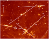 |
Fig. 1 H2 (line plus continuum) image of IC 1396N fromBeltrán et al. (2009) overlaid with the slit locations selected for this work (sX: slit; kX: knot chain). The dotted line in the bottom right corner marks the photo-ionised strip encompassed by slit A. |
3 Results
3.1 Line Kinematics
We used the molecular hydrogen lines extracted from the higherresolution spectra (grism KB) to derive some kinematical information. All lines appear unresolved in the dispersion direction, therefore the emitting gas always spans a velocity range that is narrower than the spectral resolution element (R ~ 1250, i.e. ∆V≲240 km s–1). Nevertheless, radial velocities can be obtained with a better accuracy than the spectral resolution.
We measured the wavelengths of the identified 1–0 S(0), S(1), and S(2) transitions (i.e. the brightest detected lines) by fitting Gaussian distributions to the line profiles. We assumed rest (vacuum) wavelengths of 2.223290,2.121834, and 2.033758 μm for the S(0), S(1), and S(2) transition, respectively, from Roueff et al. (2019). We then refined the wavelength calibration by measuring the radial velocities of the OH sky lines in the same (unsubtracted) frames. We identified the OH lines falling in intervals of ~0.07 μm centred around the rest wavelength of the three transitions and derived a local linear correction in each of the three intervals (the frames were all previously wavelength calibrated and straightened with the lamp spectra). The (vacuum) wavelengths of the reference sky lines were taken from Rousselot et al. (2000). The r.m.s. of the measured wavelengths minus the Rousselot wavelengths of the OH lines were ≲0.0001– 0.0002 μm (i.e. ~15–30 kms–1), confirming that the observed H2 line wavelengths can be derived with an accuracy better than the spectral resolution. Finally, the differences between observed (lamp calibrated) and theoretical H2wavelength after the OH-based correction were converted into radial velocities.
We note that the uncertainty on the radial velocities has two components. A systematic uncertainty related to the wavelength calibration, which we assume to be equal to the r.m.s. of the observed (lamp-calibrated) minus theoretical wavelengths of the comparison OH sky lines in each considered interval. And a random uncertainty, which we assume to be equal to the line width divided by the signal-to-noise ratio of each H2feature. Thus, H2features originating from the three transitions we used may have different systematic errors in the same frame. Conversely, H2features from different knots in the same frame and originating from the same H2 transition have the same systematic error and can be compared to each other with better accuracy.
The radial velocities we determined are listed in Table 2. Only those derived from the H2 1–0 S(1) transition (i.e. the feature with the best signal-to-noise ratio, S/N) are indicated. However, when the S(0) and S(2) transitions are also detected with good S/N, the derived radial velocities are consistent with each other within the errors, even more so when a shift is applied to the radial velocities obtained from the S(0) and S(2) transitions so that they coincide with that derived from the S(1) transition for the brightest knot in each frame to minimise the effects of the systematic component of the uncertainty.
One interesting result concerns knots A1 to A15 (see Fig. 2 to identify the emission features discussed in the text). As can be deduced from Table 2, the southern chain of knots (A15 south, A14, A11) are red-shifted with velocities in the range 3–50 kms–1, whereas the northern chain (A15 north, A12, A6/A7) are blue-shifted with velocities in the range –10 to –36 kms–1. This is fully consistent with the mm data from the CO(1–0) line (see Fig. 7 of Beltrán et al.2009), where blue-shifted (–3.5 to –9.5km s–1) and red-shifted (3.5–9.5km s–1) emission overlap towards the strand of knots A1–A15 and split in the eastern tip, with blue-shifted emission in the north and red-shifted emission in the south. This is evident with knot A15, a V-shaped feature that consists of two peaks that we call A15 south and A15 north. These two peaks are clearly well separated in radial velocity beyond the errors: A15 south is red-shifted and A15 north is blue-shifted. The adjoining knots A12 and A14 roughly exhibit the same velocities, suggesting that A15 south and A14 constitute a separate system from A15 north and A12. One possibility is that they are delineating a large bow shock moving eastward on the plane of the sky.
Knots C1–C17 are also consistent with CO(1–0) emission (see Fig. 2 of Beltrán et al.2012), which delineates a cavity towards C with velocities ranging from ~–10 to ~–40 km s–1 (the systemic velocity is ~0 km s–1), the same as exhibited by the knots of H2 NIR emission. Interestingly, the chain composed of knots C6, C8, and C10, facing source C of Beltrán et al. (2012), clearly consists of the most blue-shifted knots beyond the errors.
CO(1–0) emission (see Fig. 1 of Beltrán et al. 2012) indicates that knots F1–F5 should be red-shifted with radial velocities in the range 0–20 km s–1. Table 2 shows that F1 and F5 are consistent with the CO data. Nevertheless, F2 and F4 are clearly blue-shifted compared to F1 and F5 beyond the errors. This may suggest that knots F1–F5 trace an oblique shock or possibly jet precession.
For knots B1–B11, two separate chains of blue-shifted (B3, B4, and B5) and red-shifted (B7 and B8) knots are clearly identifiable. This requires further mm investigation to study the outflow structure more closely. If associated with [BGE2002] BIMA 2, as strand A is thought to be as proposed by Beltrán et al. (2009), this would confirm jet precession as suggested by its wiggled morphology.
The strand of knots G is likely to be associated with the NIR source 331 of Beltrán et al. (2009) located south-east of them. This source is also thought to originate HH 777, perpendicular to strand G, suggesting that it is a double star (Reipurth et al. 2003). The farthest knots from 331, G4 and G7, are blue-shifted, while the nearest knots become progressively more red-shifted from G1 to G3, with G3 clearly red-shifted above the errors compared to all the others. This again suggests a complex structure of the flow.
One of the slits perpendicularly encompassed a strip of emission running south-east north-west and located south-west of strand A, marking the PDR that borders the molecular cloud (hereafter the “photo-ionised strip”; it is barely visible in the bottom right corner of Fig. 1; see also Fig. 2). Interestingly, this is clearly blue-shifted compared to knots A1–A15, indicating that the heated gas in the PDR is expanding outward of the cloud.
Radial velocities (with respect to the local standard of rest) obtained from the H2 1–0 S(l) line.
3.2 Line Fluxes
The knots in strand C have the largest spectral range coverage. They were observed through both grisms HK and JH. Grism KB spectra were meant to mainly study kinematics and include several knots of strands A, B, C, F, and G (see Table 2). Finally, we used grism JH to search for [Fe ii] emission lines as well, observing knots in strands A, B, C, F, and G.
All detected spectra are composed of ro-vibrational lines of H2, and in only a few cases, of the forbidden lines [Fe ii] at 1.257, 1.320, and 1.644 μm. The measured fluxes are listed in Tables 3 and 4, normalised for each knot to the flux of the H2 1–0 S(1) line at 2.1218 μm in the HK and KB grism bands, and to the H2 1–0 S(7) line at 1.7480 μm in the JH band. We adopted the knot designation used in Beltrán et al. (2009) with a few additions as some of the line emission is from features that were not classified in Beltrán et al. (2009). Table 5 provides an updated photometry of the H21–0 S(1) line emission for the knots detected in our spectra based on the narrow-band image of Beltrán et al. (2009). This photometry can be used to calibrate the fluxes in the HK and KB grism bands (and in the JH band when the corresponding HK band spectrum is available as well). The photometry has been revised to include the knots that were previously not classified. We note that all the main physical properties of the knots can be derived from the normalised fluxes, as discussed in the next section.
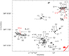 |
Fig. 2 Map of the H2 emission features in IC 1396N from the H2 2.12 μm image of Beltrán et al.(2009). The knots discussed in the text are labelled. The location of the photo-ionised strip (pis) is only indicative. |
3.3 Line Ratios
The ratio of the H2 1–0 S(1) line at 2.1218 μm to the 2–1 S(1) line at 2.2477 μm (R21) is often used to distinguish between shock-excited and UV-fluorescent H2 emission. Where the 21 line is detected (knots C, A, and G), R21 ~ 10. In other cases, lower limits (R21> 3–5) are found (see Tables 3 and 4). R21≳ 10 is usually considered an indication of shock excitation, although quiescent dense gas near to intense UV sources can yield high R21 values as well (Sternberg & Dalgarno1989). In our case, most of the knots are associated with outflows, which confirms the shock nature. For the photo-ionised strip, we obtain R21 ~ 2.1. This value is typical of radiative fluorescent emission at densities ≲104 cm–3 (Sternberg & Dalgarno1989). Even an extinction AV ~ 20 would cause R21 to be underestimated by only ~20%. Another notably difference between the photo-ionised strip and the other knots is the ratio of the H2 1–0 S(1) line to the H2 1–0 S(0) line at 2.2233 μm. Most knots exhibit a value of ~3–5, whereas the strip exhibits a ratio ~1. Both the 1–0 S(0) and the 1–0 S(2) lines display fluxes comparable to that of the 1–0 S(1) line. The main ionising source originating the PDR is the O5V star HD2006267. Assuming it is at a distance of ~13 pc from the cloud, which is the projected separation between star and cloud at a distance of 910 pc, we can estimate that the intensity in the boundary radiation field is ~100 times the average value in the solar neighbourhood (in the units used by Black & van Dishoeck 1987, with the parameters given for an O5V star by Vacca et al. 1996 and either the relation scaled to the flux at 1000 Å given by Black & van Dishoeck 1987 or Eq. (A6) of Sternberg & Dalgarno 1989). With this UV field, the models of Black & van Dishoeck (1987) predict intense fluorescently excited H2 1–0 S(0) and S(2) lines, with ratios S(0)/S(1) and S(2)/S(1) ~0.5–0.6 for molecular gas densities in the range 102–104 cm−3. The signal-to-noise ratio of the photo-ionised strip spectrum is too low to allow us to carry out a more detailed analysis, other than noting that it clearly looks different from the spectra of the other knots and is consistent with fluorescent excitation.
More accurate constraints on the physical conditions of the emitting gas can be obtained from the normalised fluxes (Tables 3 and 4) where a large number of H2ro-vibrational lines are detected. Knots C1–C17 exhibit the richest spectra, with detected H2 lines from v = 1 – 0,2 – 1,2 – 0,3 – 1,4 – 2 transitions throughout JHK (see Fig. 3), partly due to the good S/N we achieved. The S/N depends not only on knot brightness and exposure time, but also on how well the slit was positioned over the knots. Due to the blind pointing, we were not able to optimise the slit positions straight on the knots. This is easily seen in Fig. 4, which compares the KB spectra of knots A15, B8, C14, F5, and G3. Clearly, the better the S/N, the higher the number of detected transitions. We used the H2 1–0 S(6), S(7), S(8), and S(9) lines at 1.7880, 1.7480,1.7147, and 1.6878 μm, respectively, to inter-calibrate the JH and HK spectra of knots C1–C17. The fluxes were weighted according to their spectrophotometric errors. In a few cases, these four lines exhibit slightly different ratios between JH and HK, partly because S(6) and S(7) lie in a region in which atmospheric absorption is more critical (see Fig. A.1). However, this also indicates that the slit positions in JH and HK were slightly different. We note again that the slit was set on the image field by using fixed position angles and reference stars (the knots are too faint to set the slit directly). The complete spectrum of knot C14 is shown in Fig. 3 as an example.
In principle, line ratios of H2 transitions originating from the same upper level can be used to derive the extinction towards a knot. In our case 1–0 S(i) and 1–0 Q(i + 2), and 2–1 S(i) and 2–0 S(i) might be suitable. Unfortunately, each pair of lines provides different results because either one of the transitions is faint or falls in a region in which atmospheric correction is important, for instance, Q(i + 2), or the line ratio is affected by the JH-HK inter-calibration error. In addition, this computation requires that a knot has at least been observed through the HK grism. The KB grism band encloses no suitable line pairs. However, all H2detected lines can be used to simultaneously derive the excitation temperature Tex and the extinction AV minimising the uncertainty. Assuming that the gas is thermalised, the points in a ro-vibrational diagram plotting ln[I/(ɡu,JAv,j)] versus Ev,J (i.e. a so-called Boltzmann plot) are aligned in a straight line provided the line flux I has been corrected for extinction. In our notation, Av,j is the ro-vibrational transition probability, Ev,j is the energy of the upper level, and ɡv,J is the statistical weight. As the line slope depends on Tex, a simple linear fit, varying AV, simultaneously provides the best approximating Tex and AV. By adopting the extinction law of Rieke & Lebofsky (1985) in the form prescribed by Nisini et al. (2005), which is based on Draine (1989), using the transition probabilities given in Turner et al. (1977) and deriving Ev,J from Huber & Herzberg (1979), we performed the fit for knots C1–C17 with full JHK coverage, using only the points with S/N > 3. These fits are shown in Fig. 5.
The obtained Tex (2000–3000 K) is typical of H2 emission of knots from Class 0 and Class I sources (see e.g. Caratti o Garatti et al.2006). To evaluate the reliability of the linear fits, we repeated them by using the lines that fell in only one of the HK, JH, and KB grism bands. By limiting the fit to the HK band, we obtained a slightly lower Tex with an either similar to or at most ~2 mag higher AV. We note that a few spectra from which we derived AV ~ 0 yield the lowest χ2 for negative values of AV, which is unphysical. As sometimes this occurs when the band is limited to HK as well, which means that it is not always caused by the addition of the JH band, a possible explanation is that emission from higher vibrational levels originates in warmer gas. A gas stratification with different temperatures has been noted by Caratti o Garatti et al. (2006) for example. When we limit the fit to the JH points, we obtain significantly higher temperatures with an extinction either similar to or different by about ±2 mag, confirming that the emission from higher vibrational levels may arise from hotter gas. By limiting the fit to the points in the KB grism band, we obtain slightly lower Tex (by few 10%) than when the whole JHK band is used, usually (but not always) with largely overestimated extinctions, provided that the vibrational 2–1 transitions are also detected. Thus, the KB grism band only is not suitable to constrain the extinction. This is plausible because the KB grism band does not contain pairs of transitions originating in the same upper level.
Another interesting feature is evident in Fig. 4. Knots A15, F5, and G3 exhibit a more intense H2 1–0 S(3) line (1.9576 μm) than the S(1) line. The knots in strand A display S(3) lines that are even a factor of >2 brighter than the S(1) line after telluric correction. J-shock (e.g. Smith 1995) and fluorescent excitation (Sternberg & Dalgarno1989) models may both exhibit H2 1–0 S(3) lines that are slightly brighter than the S(1) transition, but possibly not such high ratios. The telluric correction of H21–0 S(3) must therefore be investigated. This line falls inside a telluric CO2 band (Fermi triad). Fig. A.1 shows that this band causes the largest absorption between ~2.05–2.07 μm, far from the S(3) line. However, this region is in the wing of the deep water absorption separating the H and K bands, so it can be affected by large water vapour variations. Table C.1 compares the S(3)/S(1) line ratios, both corrected and uncorrected for telluric absorption, for all knots in each frame. For each frame, a comparison is also displayed with the telluric star spectrum used for the correction. Although a difference in atmospheric water vapour content between the telluric star and frame A observations can explain part of the line ratio, high line ratios are obtained throughout the night, regardless of the telluric spectrum. In addition, Caratti o Garatti et al. (2006) found S(3)/S(1) line ratios of ~2 for knots A1–A15 and ~1.4 for knots B1–B11 (see their Table 22), as well as ratios >1 in several other regions. The problem may be inherent in the telluric correction method, maybe related to the intrinsic absorption hydrogen Brackett line Br8 in the telluric star spectrum near to the H2 1–0 S(3) line. In this case, the corrected H2 1–0 S(3) line flux would be systematically overestimated for all knots. Nevertheless, we verified that there is no significant difference in telluric correction in the S(3) region between using the A0 or the G2 telluric star.
We note that line ratios from different knots in the same frame can be compared to each other regardless of the telluric correction, that is, ratios normalised to that of a reference knot do not depend on atmospheric correction. Knots A1–A15 clearly display the highest S(3)/S(1) ratios. A check of the 2D spectra that were not corrected for telluric extinction also confirms that the emission in a few of these knots is dominated by the S(1) and S(3) lines in the KB grism band. If knots C1–C17 are only slightly extincted this may indicate different excitation or physical conditions for knots A1–A15. The JH spectra of knots A1–A15 do not exhibit H2 lines in the J band, maybe due to extinction, and the lines in the H band cannot be inter-calibrated with the lines in the KB grism band. The photo-ionised strip also exhibits a high S(3)/S(1) ratio, which may be accounted for by the ongoing H2 formation mechanism, as discussed above.
We detected [Fe ii] lines only towards knots A7, A11, A12, C14, and O1, confirming the results of Caratti o Garatti et al. (2006), who clearly found [Fe ii] emission at 1.644 μm from A1, A7, A11, A10-A12, and HH 593, but not towards knots C1– C17 (see their Fig. 17). In addition, knots A7, A11, A12, and O1 do not exhibit H2 lines in the J band. Emission in the [Fe ii] 1.644 and 1.257 μm, which arises from the same upper level, is intense enough to allow us to derive the extinction to those knots following the prescriptions by Pecchioli et al. (2016). For C14, both the 1.257 and the 1.320 μm lines fall in a region with relatively intense H2 ro-vibrational lines, making it difficult even to estimate upper limits. For the other knots, we found AVin the range 5–10 mag, which is consistent with AV = 10 ± 5 quoted by Caratti o Garatti et al. (2006) for knots A1–A15 and knots B1–B11. Thus, our detection of H2 lines in the J band towards knots C1–C17 and their lack towards knots A1–A15 and knots B1–B11 is consistent with the hypothesis that knots C1– C17 are less extincted than knots A1–A15 and knots B1–B11. Caratti o Garatti et al. (2006) reported, based on a sample of various star-forming regions including some of knots A1–A15 and B1–B11, that bright H2 lines in the Jband are generally observed where AV < 5 and undetected where Av > 10. On the other hand, the [Fe ii] line emission and the high S(3)/S(1) ratios towards the more extincted knots A1–A15 both clearly indicate different excitation mechanisms between knots C1–C17 and knots A1–A15 (C shocks versus J shocks?).
The excitation temperature and extinction derived from the fit to the H2 lines and the [Fe ii] line ratios are listed in Table 6. We recall the caveats noted above when only part of the JHK band is available. We also note that where the H21–0 S(3) line is much brighter than the H2 1–0 S(1), this has not been used for the fit.
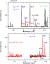 |
Fig. 3 HK and JH spectrum of knot C14. The flux scale in HK (black) is normalised to the peak flux density of the H2 1–0 S(1) emission, and the JH spectrum (red) has been scaled such that line H2 1–0 S(7) exhibits the same normalised flux in the JH and HK spectra. The identified molecular hydrogen ro-vibrational lines are indicated. |
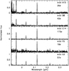 |
Fig. 4 Comparison of the KB spectra of knots A15, B8, C14, F5, and G3. The ratio of the H2 1–0 S(1) peak flux density and the r.m.s. in the adjacent spectral regions is indicated in each panel. |
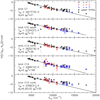 |
Fig. 5 Ro-vibrational plots (Boltzmann plots) of the H2 lines from knots C1–17, with full JHK coverage. Open black squares mark transitions from the upper vibrational level v = 1, open red circles transitions from v = 2, open blue triangles transitions from v = 3, and full black triangles upper limits for various undetected transitions. The straight lines mark the best linear fits obtained for both the excitation temperature and the extinction simultaneously. The data displayed have been corrected for the extinction value providing the best fit. The obtained temperature, extinction, and reduced χ2 are also indicated in each panel. |
Excitation temperature, extinction, and reduced χ2from fits to the H2lines (plus AVfrom [Fe ii] line ratios).
3.4 H2 Luminosities
After we derived a suitable range for extinction and excitation temperature, we used the H2 2.12 μm line fluxes from Beltrán et al.(2009) and the ratio of flux at 2.12 μm to total H2ro-vibrational lines flux computed by Caratti o Garatti et al. (2006) assuming LTE conditions to constrain the total H2luminosity of the various knots. From Table 6, we assumed Tex = 24002700 K and Avin the range 0–2 mag for C, 5–10 mag for A and B, and 2–10 mag for G. The extinction correction is based on the reddening law by Rieke & Lebofsky (1985). As for knots C1–C17, AV= 2 appears as a conservative upper limit for most of the knots, but to estimate the extinction range of G, we took into account that the extinction is usually overestimated from fitting the H2lines in the KB grism band alone. The ranges of total H2luminosities, which also assume isotropic emission, are listed in Table 7. The luminosities of the single knots provided in Table D.1 were summed to derive the values in Table7.
The total H2luminosity of knots C1–C17 is clearly comparable to that of knots A1–A15 and B1–B11. Using the relation derived by Caratti o Garatti et al. (2006), this luminosity could be associated with a driving source of Lbol ~ 13–25 L⊙. This would indicate that the two driving sources in which knots C1– C17 originate, source C and source I (Beltrán et al.2012), are solar-mass protostars, or even sub-solar mass protostars if the emission towards C is enhanced due to the outflow collision. This is also consistent with the outflow mechanical luminosities derived from CO(1–0) by Beltrán et al. (2012). When the same relation is applied to this, the driving source producing strand G should have a bolometric luminosity of 0.4-2 L⊙, that is, it would be a low-mass protostar.
Total H2 luminosity obtained assuming the extinction range indicated, Tex = 2400 –2700 K, LTE conditions, and isotropic emission (scaled to a distance of 910 pc).
4 Discussion
4.1 Strands A and B
The most remarkable result from the kinematical information (see Sect. 3.1) are the nearby knots in the same strand with significantly different radial velocities (strands A, B, and G). The simplest inference is that these jets lie roughly on the plane of the sky and do not indicate an overlap of jets from different driving sources.
In this respect, the most notable example is probably knot A15, which resembles a bow shock whose wings exhibit different radial velocities, as described above. We compared A15 with the 3D models of bow shocks by Gustafsson et al. (2010). The knot spans ~4 in width, which means ~3600 au at a distance of 910 pc. Assuming that each of the wings is ~1 in radius, which is an upper limit, we obtain from Table 5 that A15 north, for instance, has a mean brightness of ~3.5-6 ☓ 10−7 Wm2 sr−1 (which is a lower limit) after correcting for AV= 5–10. This is consistent with a bow shock seen almost edge-on that propagates in a medium with a density of ~104–105 cm−3 with a velocity of 40–60km s−1. Both the excitation temperature (~2400 K, see Table 6) and the 2–1 S(1)/1–0 S(1) ratio (~0.17 in the north and ~0.14 in the south, see Table 3) are accounted for by the models as well. Gustafsson et al. (2010) also predicted that the wings of the bow shock exhibit a different radial velocity if the magnetic field does not lie in the plane of the sky. The larger difference arises when the projected magnetic field is roughly perpendicular to the direction of propagation. The projected magnetic field derived by Soam et al. (2018) is even almost parallel to the apparent axis of A15, but this holds for the edge of the cloud, so it is likely that the orientation inside the cloud may be different. Most of the cases shown in Gustafsson et al. (2010) adopt a magnetic field strength of 500-1600 μG (in the density range of our interest), whereas Soam et al. (2018) estimated a magnetic field of 220 μG towards IC 1396N. Again, this estimate holds at the tip of the cloud, not in the inner regions. Thus, the main problem is that the velocity difference predicted for the cases examined by Gustafsson et al. (2010) is lower than 10 km s−1, while we can deduce a difference of few times 10 km s−1 from Table 2. In addition, the model parameter space should be explored in more detail to determine not only whether this velocity difference can be matched, but also whether the structure on a slightly larger scale, with the knots trailing A15 north and A15 south exhibiting a similar velocity difference, can be reproduced. Interestingly, if A15 represents a real bow shock, then its axis points towards a position in between [BGE2002] BIMA 2 and [BGE2002] BIMA 3, rather than towards [BGE2002] BIMA 2, which is the driving source that is clearly indicated by the mm outflow.
The knots in the south-western part of strand A (A1, A4, A8, and A11) exhibit the same radial velocity within the errors, a value between the extremes of A15 north and A15 south. When the systematic error is considered, this value is consistent with the velocity of the blue lobe of the outflow seen at mm wavelengths that overlaps the strand (see Fig. 6, adapted from Fig. 7a of Beltrán et al. 2009). This suggests that these knots are associated with the same flow that causes A15. [Fe ii] line emission has been observed towards some of the knots, indicating the presence of J shocks in a few areas; in particular, Caratti o Garatti et al. (2006) also found emission ahead of A15 north, as expected if this bow-shock knot represents the apex of the flow. Neither Caratti o Garatti et al. (2006) nor we detected [Fe ii] line emission towards A15 south.
An alternative explanation for the different radial velocities of A15 north and south is jet rotation. The peaks of the two knots are -2’’ apart and the difference in radial velocity is >50 km s−1 (a lower limit that takes the systematic error into account and assumes that the outflow lies on the plane of the sky). This would indicate a rotation velocity of >25 km s−1 at a distance -1″ (i.e. 910 au) from the outflow axis. Such a high rotational speed so far away from the driving source would suggest that a rotational signature should be detected in the mm outflow near to the source as well. Figure 6 (or Fig. 7 of Beltrán et al.2009) indeed shows that blue-shifted and red-shifted mm emission do not overlap near [BGE2002] BIMA 2. However, if this were the case, rotation would occur in the opposite direction compared to what is derived from knot A15. In addition, purely hydrodynamic simulations of rotating jets do not reproduce the morphology of strand A and indicate that jet rotation signatures are only preserved close to the driving source (Smith & Rosen 2007). Since a new analysis of the old mm data is beyond the scope of this work, we just note that the available NIR and mm observations both show how complex the scenario towards strand A is. Further high-resolution observations are required.
Strand B is located east of strand A and is composed of a chain of knots that is roughly aligned in an east-west direction. The radial velocity increases from west to east, ranging from ~−15 km s-1 (knot B3) to ~11 km s−1 (knot B8). Even when the systematic error is taken into account, these radial velocities are close to the systemic velocity, indicating that the knots move near to the plane of the sky. This would confirm that strand B may be part of the same outflow system that causes strand A, as suggested in the literature (Beltrán et al.2009). Other similarities between B and A are the H2luminosity (B is roughly twice as luminous as A, see Table 7) and the extinction range. Strand B exhibits a wiggled morphology that may result from jet precession, which would explain the radial velocity variations along the strand as well. The strand is -1′ in length (i.e. ~0.26 pc, or ~54000 au, at 910 pc) and assuming a projected velocity of 100 km s−1 this results in a precession period of <2600 yr.
If strands A and B are caused by the same jet (driven by [BGE2002] BIMA 2), then the jet is precessing. This link is in principle indicated by the mm CO emission outlining the outflow, which stretches from A to B but does not overlap B (see Fig. 6, adapted from Fig. 7a of Beltrán et al.2009). To further study this scenario, we tried fitting the function given by Eisloffel et al. (1996) to the positions of the knots in strands A and B from Beltrán et al. (2009). The free parameters in this simple model are the precession amplitude α,the precession length scale λ, the position angle ψof the outflow axis on the plane of the sky, and the initial phase ϕ0at the driving source. As shown in Fig. 6, our best fit does not account simultaneously for the spatial arrangement of the two strands. We tried to constrain some of the free parameters as well, but were unable to find a better visual agreement. In Table 8 we list the parameters obtained from the fits to strand A, to strand B, and to strand A and B simultaneously, all assuming [BGE2002] BIMA 2 as the driving source. Clearly, if [BGE2002] BIMA 2 did cause strands A and B, then a simple jet precession is not sufficient to explain their locations. One possible scenario is that an event between the ejection of B and A has resulted in changing the jet position angle, increasing the amplitude and decreasing the timescale of the precession (see Table 8). This would require a close encounter of [BGE2002] BIMA 2 with another stellar object during an accretion phase (Bate et al.2000), for example. Another scenario is that strand A is caused by the interaction of two or more jets from different driving sources. Finally, A and B could have been caused by two different driving sources. At present, our data do not allow us to distinguish between these three possible interpretations.
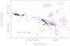 |
Fig. 6 Best fit of the projected morphology of a precessing jet as parametrised by Eisloffel et al. (1996) to the locations of the knots in strands A and B, overlaid with the H2 2.12 μm image (continuum subtracted) in grey scale and CO (J = 1 − 0) emission integrated in the [±3.5, ±9.5] km s–1 velocity interval in red and blue contours (adapted from Fig. 7a of Beltrán et al.2009). The crosses mark the location of the compact radio sources [BGE2002] BIMA 1, 2, and 3. |
Jet parameters obtained from fitting the function by Eisloffel etal. (1996) to the locations of knots A1–A15 and/or B1–B11.
4.2 Other Emission Features
The chain of knots G exhibits a radial velocity pattern similar to that of strand B. The knots are aligned in a south-east to north-west direction, and the radial velocity increases from knot G1 (−7 km s−1) to G3 (40km s−1), then decreases again to G7 (–31 km s−1). These values oscillate around a value close to the systemic velocity (i.e. ~0 km s−1), even when the systematic errors are taken into account, suggesting that in this case, the outflow also lies close to the plane of the sky. The most likely explanation is jet precession or the orbital motion of the driving source in a double system (e.g. Estalella et al.2012). If the knots are much closer than strand B to the driving source, we can expect that a wiggled morphology has not yet developed above the spatial resolution of the available images. Using the same computation as for B, we obtain a precession period of ~1300 yr. Strand G has commonly been associated with the infrared source HH 777/IRS331, which also seems to drive a perpendicular outflow originating the Herbig-Haro object HH 777 (Beltrán et al. 2009). If this is the case, HH 777/IRS331 would be a double system, and jet precession or the effects of orbital motion are both plausible.
Strand F is associated with the red lobe of the outflow from source I (Beltrán et al.2012), and its knots are therefore expected to exhibit radial velocities in the range ~0–20km s−1 (see Fig. 2 of Beltrán et al.2012). Although the radial velocity of knots F1 and F5 agrees, the knots in between, F2 and F4, are clearly blue-shifted with radial velocities of –11 and –33 km s−1, respectively. On the other hand, knots C1–C17 are associated with the blue lobes of the outflows from sources I and C and display radial velocities in the range –8 to –47km s−1, in agreement with the radial velocities obtained from the mm emission. The pattern in the radial velocities of knots F1–F5 is not easily interpreted as jet precession. Alternatively, it could be due to oblique shocks developing due to gas inhomogeneities. The detailed pattern exhibited by knots C1–C17 is more difficult to interpret as this region results from the overlap (possibly the collision) of the two different outflows. This pattern is explored in detail in a twin paper (López et al.2022) using proper motion determination.
We note that the difference (i.e. not the single values) in radial velocities between knots in the same strand never exceeds the critical speed for H2 dissociation (e.g. Gustafsson et al. 2010), which confirms that each strand represents one single system and did not originate from the overlap of different jets.
The most notable result from the excitation analysis of the H2emission from the knots in strand C is that they appear to be less extincted than the other features in the cloud. This suggests that they are closer to the cloud surface facing the observer. We detected [Fe ii] emission only towards knot C14, the brightest in the strand (see Table 5), although we would expect more widespread [Fe ii] emission if the outflow-collision scenario were correct. In this respect, a clue might come from the presence of higher temperature gas, which unfortunately is only hinted at by our data.
The only other knot in which we detected [Fe ii] emission is O1, which also exhibits a high H2 1–0 S(3)/S(1) flux ratio, as found towards A. It is a highly reddened (Av~ 7) red-shifted (~22 km s−1) isolated feature aligned with strand F. This is consistent with O1 being a terminal shock associated with the red lobe of the outflow driven by source I.
The photo-ionised strip borders the south-western rim of the dark optical nebula (see e.g. Fig. 1 of Codella et al.2001) and is roughly perpendicular to the direction to HD20626. A patch of blue-shifted molecular gas was observed towards this part of the dark nebula (see Fig. 3 of Codella et al.2001); its radial velocity, ~–5kms−1, coincides with the radial velocity we measured for the strip (see Table 2) within the errors. Its H2emission therefore marks the PDR facing the ionising source, seen edge-on. Its blue-shifted radial velocity is likely to be the signature of a photo-evaporation process. However, a PDR should expand at the sound speed of the warm gas (a fewkms−1; Gorti & Hollenbach2002), hence the H2radial velocity we found, if confirmed, cannot be accounted for by gas expansion alone.
4.3 Jets from Sources in Orbital Motion
An alternative to jet precession is that the driving source is in orbital motion in a double system, as we described above. Although in some cases the two scenarios may be hardly distinguishable (e.g. see Ferrero et al.2022), we can show that this can probably be ruled out for strand A. Based on the simple formulation by Masciadri & Raga (2002), if the driving source is located towards [BGE2002] BIMA 2, we can estimate the orbital radius r0 from their Eq. (13) (under the assumption of a circular orbit) deriving ∆z from our Fig. 6 (~35″) and a lower limit for k = tanαfrom Table 8(α~ 9°). Then, we can estimate a minimum mass Mp for the driving source from their Eq. (1), using a period T ~ 2000 yr from Table 8 and noting that Mp is minimum when Mp/Ms = 1 (Mp ≥ Ms). We obtain Mp⪞ 500 M⊙, which is clearly inconsistent. We conclude that the morphology of strand A cannot be produced by a driving source that coincides with [BGE2002] BIMA 2 and is in orbital motion.
5 Summary and Conclusions
We have presented long-slit NIR J, H, and K spectroscopy of the H2 outflows reported by Beltrán et al. (2009) in the bright-rimmed cloud IC 1396N. The analysis of the spectra allowed us to derive physical properties (from the grisms spanning the JH and HK bands with R ~ 500 and the grism spanning the K band with R ~ 1200) and kinematics (from the grism spanning the K band with R ~ 1200) for the knots encompassed by the slit (using several pointings and position angles). The main results are listed below:
The spectra of the jet knots show a set of ro-vibrational lines of H2 and [Fe ii] forbidden lines. The [Fe ii] lines are only detected towards knots A7, A11, A12, C14, and O1.
We derived the radial velocity of the jet knots from the H2 1–0 S(1) transition. In addition, we verified that the radial velocities derived from the S(0) and S(2) transitions (where these lines are detected with a good S/N) are consistent within the errors with the S(1) results.
We found blue-shifted and red-shifted radial velocity values ranging from –40 to +50 km s–1. For the strands of knots A and C, the blue-shifted and red-shifted emission is fully consistent with the mm data from the CO emission of Beltrán et al. (2009, Beltrán et al. 2012).
Knots F1–F5 lie in the red-shifted lobe of one of the CO outflow. We found red-shifted velocities for knots F1 and F5, in agreement with CO data, while F2 and F4 have blue-shifted velocities. Knots B1–B11 and G1–G7 show two separate chains of blue-shifted and red-shifted knots.
The simultaneous presence of blue-shifted and red-shifted knots in the same strands indicates that the outflows roughly lie on the plane of the sky. It also suggests that jet precession is ubiquitous in the region, as was confirmed by the wiggling morphology of strand B, for example.
A photo-ionised strip, located south-west of strand A, marks the edge-on PDR at the side of the cloud facing the ionising star and displays a blue-shifted velocity, which may (at least partly) be accounted for by gas photo-evaporation.
The H2 line ratios 1–0 S(1) to 2–1 S(1), and 1–0 S(1) to 10 S(0) were used to distinguish between shock-excited and UV-fluorescent mechanisms giving rise to the H2 emission. The ratios we found for the knots of the chains we mapped are consistent with shock excitation as expected for the emission of knots associated with H2 outflows. These line ratios are significantly different for the photo-ionised strip southwest of the chain of knots A, which confirms a fluorescent mechanism of the emission.
We used all the H2 detected lines to simultaneously derive the excitation temperature (Tex) and the extinction (AV) assuming that the gas is thermalised. The Tex obtained (2000–3000 K) is typical of H2jet knots from Class 0 and ClassIsources. We found that the chain of knots C has a lower extinction (AV in the range of 0–2 mag) than chains A, B (5–10 mag), and G (2–10 mag). This is consistent with the lack of detection of H2 lines in the J band toward knots A1–A15 and B1–B11, while these lines are detected in knots C1–C17. In addition, the higher-excitation lines indicate higher-temperature layers of gas.
The detection of [Fe ii] lines and the high H2 1–0(3)/S(1) ratios towards the more extincted knots of the A chain and O1 indicate that different excitation mechanisms (C shocks versus J shocks) cause the emission from knots C1–C17, 01,and A1–A15. However, because the H21–0 S(3) wavelength coincides with a spectral region in which atmospheric extinction is an issue, the ratio H2 1–0 S(3)/S(1) in these (and similar other features in a number of regions) deserves further investigation. Our data strongly suggest that the high values of this ratio are real.
We derived the total H2 luminosity of the knots, assuming LTE conditions and the ranges of AV and Tex found previously. The luminosities of strand C are consistent with the hypothesis that the mm sources I and C of Beltrán et al. (2012) are solar or sub-solar mass (proto)stars.
We found that a simple precession model cannot account for the hypothesis that strands A and B both originate from source [BGE2002] BIMA 2, as suggested in the literature. We also ruled out that the outflow morphology results from a driving source in orbital motion towards [BGE2002] BIMA 2,which would need to possess an inconsistently high mass. This indicates either a more complex scenario or that these strands are not produced by the same driving source.
By comparing strand A with numerical 3D models, we determined that the eastern tip of the strand is consistent with a bow shock leading an outflowing parcel of gas. Knot O1 is likely to represent a terminal shock associated with strand F and the red lobe of the outflow from mm source I.
Further high spatial-resolution mm observations are needed to study the relation (if any) between strands A and B and find out the exact origin of the radial velocity oscillations displayed within some of the strands.
Acknowledgements
This work has been partially supported by the Spanish MINECO grants AYA2014–57369–C3 and AYA2017–84390–C2 (co-funded with FEDER funds) and MDM-2014–0369 of ICCUB (Unidad de Excelencia ‘María de Maeztu’). We would like to thank the referee, A. Raga, for his insightful comments.
Appendix A Atmospheric Transmission
We used the ESO Advanced Cerro Paranal Sky Model2(Noll et al. 2012) to build a picture of the atmospheric transmission in the JHK bands and identify the more critical wavelength ranges for spectroscopy (Fig. A.1). Lines falling in the wings of the water telluric absorption features separating the JHK bands clearly need to be considered with caution, especially because the transmission in these regions can be highly variable.
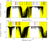 |
Fig. A.1 Atmospheric transmission in the bands spanned by grism HK (top panel) and JH (bottom panel). The vertical bars indicate the wavelengths of the H2 lines (black) and [Fe ii] lines (red) discussed in the main text. The yellow areas mark the wavelength ranges within which correction for atmospheric extinction may exhibit large errors. The range spanned by grism KB is limited by the vertical dashed lines. |
Appendix B Telluric Correction
We performed a simple test of the accuracy of our telluric correction by dividing pairs of 1D spectra of the same telluric standard star taken at different times during the same night. This clearly removes the intrinsic stellar spectrum, and the obtained curve, r(/λ) [= T1(λ)/T2(λ)], allows mapping the differences in flux ratios between two wavelengths when the telluric correction curve derived from one of the two stellar spectra rather than the other is used. In particular, if a wavelength λa is selected as a reference (we used 2.1 μm for grisms KB and HK, and 1.7 μm for grism JH), we can derive the difference in the flux ratio Ri(λa, λb) [= S (λb)/S (λa)] of two hypothetical lines centred at λa and λb when using either the first (R1) or the second (R2) stellar spectrum to correct for a target spectrum. The quantity r(λ) typically has an average value ~1 and exhibits small oscillations or even a slight gradient. The average value is not relevant for the line ratios because its variations are due to seeing changes, pointing inaccuracies, different airmasses, and so on during the two integrations on the telluric stars. The average value does not affect the line ratios because
 (B.1)
(B.1)
yields the relative difference in the ratios of flux at λband at our reference wavelength λa between the two corrections.
Standard spectral ratios r between pairs of stellar spectra in the same ABBA cycle indicate flux ratio changes of at most ~5% in the HK and KB grism bands, and ~ 10% in the JH band. Thus, we averaged all four 1D spectra from any ABBA cycle before constructing the associated telluric correction curve (Sect. 2). No significant difference is found between the correction spectra obtained from the A0V and the G2V stars. Finally, even the ratios r obtained from the average spectra taken at the beginning, in the middle and at the end of a night, point to maximum line ratio differences of ~ 10% when both lines fall outside the regions of strong telluric absorption (see Fig. A.1), particularly water.
The telluric lines or bands at ~1.24–1.28 μm (O2), ~1.56– 1.6μm (CO2 and O2), ~2–2.08 μm (CO2), ~1.65–1.7 μm and ~2.24–2.3 μm (CH4) showed variations during the same night that are mostly related with the airmass, as expected. The maximum flux ratio changes were found for λbcoinciding with the wavelength of the peak of the strongest CO2 absorption line at ~2 μm (~30% for an airmass difference of ~0.4) and for λbinside the range of the O2 band at ~ 1.24–1.28 μm (~25% for an airmass difference of ~0.4).
Appendix C Telluric Correction at the Edge of the KB Grism Band
A puzzling result is the high value of the ratio H2 1–0 S(3)/S(1) measured towards some of the knots. Table C.1 compares the ratios before and after telluric correction for every knot in each KB grism frame and lists their relation with the telluric standard star we used.
Appendix D  of single knots
Table D.1 lists the total luminosity in H2ro-vibrational transitions of single knots derived from the photometry of H2 1–0 S(1) line emission at 2.12 μm given by Beltrán et al. (2009). The computation assumes the Tex and AV ranges deduced in Sect. 3.3 through linear fits in the Boltzmann plots to the detected H2 lines or through [Fe ii] line ratios, the extinction law of Rieke & Lebofsky (1985), LTE conditions, and isotropic emission from the knots. We used the relation between total H2 and H2 1–0 S(1) fluxes in LTE as a function of Tex computed by Caratti o Garatti et al. (2006).
References
- Baffa, C., Comoretto, G., Gennari, S., et al. 2001, A&A, 378, 722 [NASA ADS] [CrossRef] [EDP Sciences] [Google Scholar]
- Bate, M. R., Bonnell, I. A., Clarke, C. J., et al. 2000, MNRAS, 317, 773 [NASA ADS] [CrossRef] [Google Scholar]
- Beltrán, M. T., Girart, J. M., Estalella, R., Ho, P. T. P., & Palau, A. 2002, ApJ, 573, 246 [CrossRef] [Google Scholar]
- Beltrán, M. T., Massi, F., López, R., Girart, J. M., & Estalella, R. 2009, A&A, 504, 97 [NASA ADS] [CrossRef] [EDP Sciences] [Google Scholar]
- Beltrán, M. T., Massi, F., Fontani, F., Codella, C., & López, R. 2012, A&A, 542, L26 [NASA ADS] [CrossRef] [EDP Sciences] [Google Scholar]
- Black, J. H., & van Dishoeck, E. F. 1987, ApJ, 322, 412 [Google Scholar]
- Caratti o Garatti, A., Giannini, T., Nisini, B., & Lorenzetti, D. 2006, A&A, 449, 1077 [NASA ADS] [CrossRef] [EDP Sciences] [Google Scholar]
- Choudhury, R., Mookerjea, B., & Bhatt, H. C. 2010, ApJ, 717, 1067 [NASA ADS] [CrossRef] [Google Scholar]
- Codella, C., Bachiller, R., Nisini, B., Saraceno, P., & Testi, L. 2001, A&A, 376, 271 [NASA ADS] [CrossRef] [EDP Sciences] [Google Scholar]
- Draine, B. T. 1989, in Infrared Spectroscopy in Astronomy, ed. E. Böhm-Vitense, 93 [Google Scholar]
- Eisloffel, J., Smith, M. D., Davis, C. J., & Ray, T. P. 1996, AJ, 112, 2086 [NASA ADS] [CrossRef] [Google Scholar]
- Estalella, R., López, R., Anglada, G., et al. 2012, AJ, 144, 61 [Google Scholar]
- Ferrero, L. V., Günthardt, G., García, L., et al. 2022, A&A, 657, A110 [NASA ADS] [CrossRef] [EDP Sciences] [Google Scholar]
- Getman, K. V., Feigelson, E. D., Garmire, G., Broos, P., & Wang, J. 2007, ApJ, 654, 316 [NASA ADS] [CrossRef] [Google Scholar]
- Gorti, U., & Hollenbach, D. 2002, ApJ, 573, 215 [Google Scholar]
- Gustafsson, M., Ravkilde, T., Kristensen, L. E., et al. 2010, A&A, 513, A5 [NASA ADS] [CrossRef] [EDP Sciences] [Google Scholar]
- Hollenbach, D., & McKee, C. F. 1979, ApJS, 41, 555 [Google Scholar]
- Hollenbach, D., & McKee, C. F. 1980, ApJ, 241, L47 [NASA ADS] [CrossRef] [Google Scholar]
- Hollenbach, D., & McKee, C. F. 1989, ApJ, 342, 306 [Google Scholar]
- Huber, K. P., & Herzberg, G. 1979, Spectral and Molecular Structure IV. Constants of Diatomic Molecules (New York: Van Nostrand Reinhold) [Google Scholar]
- Kaufman, M. J., & Neufeld, D. A. 1996, ApJ, 456, 611 [NASA ADS] [CrossRef] [Google Scholar]
- López, R., Estalella, R., Beltrán, M. T., et al. 2022, A&A, 661, A106 [NASA ADS] [CrossRef] [EDP Sciences] [Google Scholar]
- Maiolino, R., Rieke, G. H., & Rieke, M. J. 1996, AJ, 111, 537 [NASA ADS] [CrossRef] [Google Scholar]
- Maíz Apellániz, J., & Barbá, R. H. 2020, A&A, 636, A28 [NASA ADS] [CrossRef] [EDP Sciences] [Google Scholar]
- Masciadri, E., & Raga, A. C. 2002, ApJ, 568, 733 [Google Scholar]
- Massi, F., Codella, C., Brand, J., di Fabrizio, L., & Wouterloot, J. G. A. 2008, A&A, 490, 1079 [NASA ADS] [CrossRef] [EDP Sciences] [Google Scholar]
- Nisini, B., Massi, F., Vitali, F., et al. 2001, A&A, 376, 553 [NASA ADS] [CrossRef] [EDP Sciences] [Google Scholar]
- Nisini, B., Bacciotti, F., Giannini, T., et al. 2005, A&A, 441, 159 [NASA ADS] [CrossRef] [EDP Sciences] [Google Scholar]
- Noll, S., Kausch, W., Barden, M., et al. 2012, A&A, 543, A92 [NASA ADS] [CrossRef] [EDP Sciences] [Google Scholar]
- Pecchioli, T., Sanna, N., Massi, F., & Oliva, E. 2016, PASP, 128, 073001 [NASA ADS] [CrossRef] [Google Scholar]
- Reipurth, B., Armond, T., Raga, A., & Bally, J. 2003, ApJ, 593, L47 [NASA ADS] [CrossRef] [Google Scholar]
- Rieke, G. H., & Lebofsky, M. J. 1985, ApJ, 288, 618 [Google Scholar]
- Roueff, E., Abgrall, H., Czachorowski, P., et al. 2019, A&A, 630, A58 [NASA ADS] [CrossRef] [EDP Sciences] [Google Scholar]
- Rousselot, P., Lidman, C., Cuby, J. G., Moreels, G., & Monnet, G. 2000, A&A, 354, 1134 [Google Scholar]
- Smith, M. D. 1995, A&A, 296, 789 [NASA ADS] [Google Scholar]
- Smith, M. D., & Rosen, A. 2007, MNRAS, 378, 691 [NASA ADS] [CrossRef] [Google Scholar]
- Soam, A., Maheswar, G., Lee, C. W., Neha, S., & Kim, K.-T. 2018, MNRAS, 476, 4782 [Google Scholar]
- Sternberg, A., & Dalgarno, A. 1989, ApJ, 338, 197 [Google Scholar]
- Sugitani, K., Fukui, Y., & Ogura, K. 1991, ApJS, 77, 59 [NASA ADS] [CrossRef] [Google Scholar]
- Sugitani, K., Tamura, M., Nakaya, H., et al. 2002, in 8th Asian-Pacific Regional Meeting, II, eds. S. Ikeuchi, J. Hearnshaw, & T. Hanawa, 213 [Google Scholar]
- Turner, J., Kirby-Docken, K., & Dalgarno, A. 1977, ApJS, 35, 281 [NASA ADS] [CrossRef] [Google Scholar]
- Vacca, W. D., Garmany, C. D., & Shull, J. M. 1996, ApJ, 460, 914 [NASA ADS] [CrossRef] [Google Scholar]
- Vacca, W. D., Cushing, M. C., & Rayner, J. T. 2003, PASP, 115, 389 [NASA ADS] [CrossRef] [Google Scholar]
- Zapata, L. A., Fernández-López, M., Rodríguez, L. F., et al. 2018, AJ, 156, 239 [NASA ADS] [CrossRef] [Google Scholar]
- Zucker, C., Speagle, J. S., Schlafly, E. F., et al. 2020, A&A, 633, A51 [NASA ADS] [CrossRef] [EDP Sciences] [Google Scholar]
IRAF is distributed by the National Optical Astronomy Observatories, which are operated by the Association of Universities for Research in Astronomy, Inc., under cooperative agreement with the National Science Foundation.
All Tables
Radial velocities (with respect to the local standard of rest) obtained from the H2 1–0 S(l) line.
Excitation temperature, extinction, and reduced χ2from fits to the H2lines (plus AVfrom [Fe ii] line ratios).
Total H2 luminosity obtained assuming the extinction range indicated, Tex = 2400 –2700 K, LTE conditions, and isotropic emission (scaled to a distance of 910 pc).
Jet parameters obtained from fitting the function by Eisloffel etal. (1996) to the locations of knots A1–A15 and/or B1–B11.
All Figures
|
Fig. 1 H2 (line plus continuum) image of IC 1396N fromBeltrán et al. (2009) overlaid with the slit locations selected for this work (sX: slit; kX: knot chain). The dotted line in the bottom right corner marks the photo-ionised strip encompassed by slit A. |
| In the text | |
|
Fig. 2 Map of the H2 emission features in IC 1396N from the H2 2.12 μm image of Beltrán et al.(2009). The knots discussed in the text are labelled. The location of the photo-ionised strip (pis) is only indicative. |
| In the text | |
|
Fig. 3 HK and JH spectrum of knot C14. The flux scale in HK (black) is normalised to the peak flux density of the H2 1–0 S(1) emission, and the JH spectrum (red) has been scaled such that line H2 1–0 S(7) exhibits the same normalised flux in the JH and HK spectra. The identified molecular hydrogen ro-vibrational lines are indicated. |
| In the text | |
|
Fig. 4 Comparison of the KB spectra of knots A15, B8, C14, F5, and G3. The ratio of the H2 1–0 S(1) peak flux density and the r.m.s. in the adjacent spectral regions is indicated in each panel. |
| In the text | |
|
Fig. 5 Ro-vibrational plots (Boltzmann plots) of the H2 lines from knots C1–17, with full JHK coverage. Open black squares mark transitions from the upper vibrational level v = 1, open red circles transitions from v = 2, open blue triangles transitions from v = 3, and full black triangles upper limits for various undetected transitions. The straight lines mark the best linear fits obtained for both the excitation temperature and the extinction simultaneously. The data displayed have been corrected for the extinction value providing the best fit. The obtained temperature, extinction, and reduced χ2 are also indicated in each panel. |
| In the text | |
|
Fig. 6 Best fit of the projected morphology of a precessing jet as parametrised by Eisloffel et al. (1996) to the locations of the knots in strands A and B, overlaid with the H2 2.12 μm image (continuum subtracted) in grey scale and CO (J = 1 − 0) emission integrated in the [±3.5, ±9.5] km s–1 velocity interval in red and blue contours (adapted from Fig. 7a of Beltrán et al.2009). The crosses mark the location of the compact radio sources [BGE2002] BIMA 1, 2, and 3. |
| In the text | |
|
Fig. A.1 Atmospheric transmission in the bands spanned by grism HK (top panel) and JH (bottom panel). The vertical bars indicate the wavelengths of the H2 lines (black) and [Fe ii] lines (red) discussed in the main text. The yellow areas mark the wavelength ranges within which correction for atmospheric extinction may exhibit large errors. The range spanned by grism KB is limited by the vertical dashed lines. |
| In the text | |
Current usage metrics show cumulative count of Article Views (full-text article views including HTML views, PDF and ePub downloads, according to the available data) and Abstracts Views on Vision4Press platform.
Data correspond to usage on the plateform after 2015. The current usage metrics is available 48-96 hours after online publication and is updated daily on week days.
Initial download of the metrics may take a while.