| Issue |
A&A
Volume 664, August 2022
|
|
|---|---|---|
| Article Number | A183 | |
| Number of page(s) | 15 | |
| Section | The Sun and the Heliosphere | |
| DOI | https://doi.org/10.1051/0004-6361/202243357 | |
| Published online | 29 August 2022 | |
Impact of spatially correlated fluctuations in sunspots on metrics related to magnetic twist
1
Max-Planck-Institut für Sonnensystemforschung, 37077 Göttingen, Germany
e-mail: baumgartner@mps.mpg.de
2
School of Information and Physical Sciences, The University of Newcastle, New South Wales, Australia
3
Georg-August-Universität Göttingen, Institut für Astrophysik, Friedrich-Hund-Platz 1, 37077 Göttingen, Germany
Received:
18
February
2022
Accepted:
17
March
2022
Context. The twist of the magnetic field above a sunspot is an important quantity in solar physics. For example, magnetic twist plays a role in the initiation of flares and coronal mass ejections (CMEs). Various proxies for the twist above the photosphere have been found using models of uniformly twisted flux tubes, and are routinely computed from single photospheric vector magnetograms. One class of proxies is based on αz, the ratio of the vertical current to the vertical magnetic field. Another class of proxies is based on the so-called twist density, q, which depends on the ratio of the azimuthal field to the vertical field. However, the sensitivity of these proxies to temporal fluctuations of the magnetic field has not yet been well characterized.
Aims. We aim to determine the sensitivity of twist proxies to temporal fluctuations in the magnetic field as estimated from time-series of SDO/HMI vector magnetic field maps.
Methods. To this end, we introduce a model of a sunspot with a peak vertical field of 2370 Gauss at the photosphere and a uniform twist density q = −0.024 Mm−1. We add realizations of the temporal fluctuations of the magnetic field that are consistent with SDO/HMI observations, including the spatial correlations. Using a Monte-Carlo approach, we determine the robustness of the different proxies to the temporal fluctuations.
Results. The temporal fluctuations of the three components of the magnetic field are correlated for spatial separations up to 1.4 Mm (more than expected from the point spread function alone). The Monte-Carlo approach enables us to demonstrate that several proxies for the twist of the magnetic field are not biased in each of the individual magnetograms. The associated random errors on the proxies have standard deviations in the range between 0.002 and 0.006 Mm−1, which is smaller by approximately one order of magnitude than the mean value of q.
Key words: Sun: photosphere / Sun: magnetic fields / sunspots
© C. Baumgartner et al. 2022
 Open Access article, published by EDP Sciences, under the terms of the Creative Commons Attribution License (https://creativecommons.org/licenses/by/4.0), which permits unrestricted use, distribution, and reproduction in any medium, provided the original work is properly cited.
Open Access funding provided by Max Planck Society.
1. Introduction
The magnetic field in solar active regions is often modeled by coherent bundles of magnetic field lines, so-called flux tubes. The magnetic helicity H = ∫VA ⋅ B dV, where A is the magnetic vector potential and B is the magnetic field, can be used to describe the topological structure of flux tubes fully contained in a volume V (Berger & Field 1984). The magnetic helicity of a single flux tube has two components: writhe, which measures the deformation of its axis, and twist. If one imagines the magnetic field as a straight ribbon with its two ends rotated in opposite directions, the twist T measures how often the ribbon turns around its straight axis

where L is the length of the ribbon and q is the twist density, which counts how often the ribbon fully turns per unit length.
Measurements of the twist of magnetic field play an important role in many different areas of solar physics: The twist distribution in the photosphere constrains models of the solar dynamo and magnetic flux emergence (e.g., Gilman & Charbonneau 1999; Brandenburg 2005; Pipin et al. 2013). For example, the hemispheric helicity sign rule describes an observed latitudinal dependence of the twist with predominantly negative (counter-clockwise) or positive (clockwise) twist in the northern or southern hemisphere (Seehafer 1990; Pevtsov et al. 1995; Longcope et al. 1998; Nandy 2006), which is a key ingredient that solar dynamo models should be able to reproduce (Charbonneau 2020). The twist in the magnetic field plays an essential part in the dynamics of the solar atmosphere; for example a highly twisted flux tube can become susceptible to kink instability, which leads to a deformation of the axis of the flux tube in exchange for its twist. This is a possible trigger mechanism for solar flares and CMEs (e.g., Török & Kliem 2003; Török et al. 2004; Leka et al. 2005; Fan 2005). Furthermore, the observed twist of photospheric magnetic field is used as an input to inject twist into coronal magnetic field extrapolations (e.g., Yeates et al. 2008; Wiegelmann & Sakurai 2012).
Various methods have been developed to measure the twist density of the magnetic field in active regions directly from individual photospheric observations. These methods either use the force-free parameter, α, as a proxy for the twist density or try to fit the twist density directly.
Woltjer (1958) shows that the force-free parameter α in a closed system corresponds to the helicity content of a linear force-free field structure in its lowest attainable energy state. Therefore, α is used in observations as a proxy for the helicity of the magnetic field (Pevtsov et al. 2014).
As we have observations at only one height in the photosphere from instruments like HMI, we cannot measure α directly. We are limited to calculating the vertical current density Jz and consequently αz = Jz/Bz at one height, where Bz is the vertical field strength. Burnette et al. (2004) studied 34 active regions and show that a two-dimensional spatial average of αz over an active region is correlated with the α value corresponding to the three-dimensional linear-force-free extrapolation with the best least-squares fit to the observed field. Therefore, spatial averages of αz are often used to characterize the helicity and twist of the magnetic field in active regions or individual sunspots (e.g., Longcope et al. 1998; Hagino & Sakurai 2004). Leka et al. (2005) chose a single peak value of αz close to center the of a sunspot (αPeak) to characterize the twist in the magnetic field. This is because in simple models αz only relates directly to the twist density at the axis of a flux tube (αPeak = 2q).
Nandy et al. (2008) suggested a method to infer the twist density of the magnetic field q that avoids the force-free assumption. These authors assume that the magnetic field in a sunspot can be approximated by a monolithic vertical flux tube with a constant twist density. They then use a least-squares fitting approach to fit the observations to this reference model to obtain the twist density.
Various tests of these methods have been conducted. Leka & Skumanich (1999) and Leka (1999) used observations to compare methods of using moments of the distribution of αz, a global α from force-free extrapolations, and a fitting approach of the function Jz = αBz. These authors find quantitative agreement between these methods. They also assessed the influence of instrumental effects like spatial resolution and a limited field-of-view, and considered noise by restricting the αz measurements to certain noise thresholds. Leka et al. (2005) successfully retrieved the twist density using their αPeak method on a model by Fan & Gibson (2004) in the absence of errors. Crouch (2012) evaluated different least-squares fitting methods of the twist density from a model flux tube, and find that the inferred twist density can be significantly different depending on the model assumptions used for fitting, also in the absence of noise. Tiwari et al. (2009a) used a linear force-free magnetic field model to test the effect of random polarimetric noise on estimates of the global α value of the synthetic field structure. They find that noise does not influence the sign of α and the global twist can be measured accurately.
To interpret twist density measurements from a single observation, we need to understand how these measurements are affected by temporal variations of the magnetic field. HMI observes the magnetic field in the photosphere where the force-free assumption is thought to be violated (Gary 2001). Temporal fluctuations of the magnetic field may arise in such an environment; for example a twisted magnetic field structure can be distorted by its surrounding plasma flows. We need to model the fluctuations of the magnetic field in a sunspot from SDO/HMI observations to characterize the sensitivity of twist measurements to these fluctuations.
We tested the robustness of existing methods to infer the twist of the magnetic field under temporal variations of the magnetic field from SDO/HMI observations. We modeled the well-established leading sunspot of active region NOAA 11072 (observed by SDO/HMI at 2010.05.25 03:00:00 TAI) with the semi-empirical sunspot model by Cameron et al. (2011) with added uniform twist. We studied the spatial covariance of the temporal fluctuations of the magnetic field and created a model based on our findings. We tested the robustness of methods to measure twist using Monte-Carlo simulations of the sunspot and fluctuation model.
In Sect. 2 we present vector magnetic field observations of the reference sunspot in active region NOAA 11072. Sections 3 and 4 describe the fluctuation and sunspot model, respectively. In Sect. 5 we present a summary of the twist measurement methods that we test in this paper as well as their implementation. We then qualitatively compare our sunspot model to the SDO/HMI observations of the reference sunspot in Sect. 6. In Sect. 7 we present Monte-Carlo simulations to test how the twist measurement methods fare under the influence of temporally fluctuating magnetic field.
2. SDO/HMI vector magnetogram observations of our reference sunspot in active region NOAA 11072
In this section, we present a sunspot observed by SDO/HMI that we selected as a reference for our sunspot model. The reference sunspot should closely resemble the assumption that its magnetic field structure could be described as a monolithic uniformly twisted flux tube. Therefore, we looked for sunspots that are well established, roughly circular, and under little influence from other strong magnetic field in its vicinity. We model the sunspot with uniform twist to test various methods to measure the twist under temporal fluctuations of the magnetic field.
We chose the leading sunspot of active region NOAA 11072 (2010.05.25 03:00:00 TAI), which was located about 30° away from disk center at the Stonyhurst heliographic coordinates 27° east and 13° south. Figure 1 shows the Postel-projected sunspot transformed to local cylindrical coordinates from SDO/HMI vector magnetogram observations (hmi.b_720s, Hoeksema et al. 2014). Bz is the component normal to the surface. Br and Bθ are located in a plane parallel to the surface. Br points radially away from the center of the spot and Bθ is always perpendicular to Br. See Appendix A for a detailed description of the coordinate systems and transformations used.
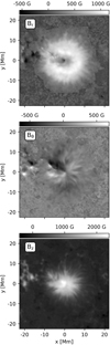 |
Fig. 1. SDO/HMI vector magnetogram of the leading sunspot of active region NOAA 11072 (2010.05.25 03:00:00 TAI) in cylindrical coordinates. Br (top), Bθ (middle), and Bz (bottom) show the radial, azimuthal, and vertical component of the magnetic field. |
The sunspots we considered have a dominant radial Br and weak azimuthal Bθ component, as shown for the example of the reference sunspot in Fig. 2. This is a known characteristic of sunspots (Borrero & Ichimoto 2011). We noticed that the azimuthal component – which carries information about the handedness of the twist in a uniformly twisted flux tube – shows that the sunspot has regions with opposite sign of twist.
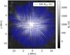 |
Fig. 2. SDO/HMI vector magnetogram of the leading sunspot of active region NOAA 11072 (2010.05.25 03:00:00 TAI) with the horizontal field Bhor plotted as arrows on top of the vertical vector component Bz. |
3. Estimating the spatial covariance of magnetic field fluctuations from the observations
We aimed to derive a model for the temporal fluctuations of the magnetic field in SDO/HMI vector magnetogram observations. To do so, we used an approximately seven-hour time-series of our reference spot (2010.05.25, 03:00:00−9:48:00 TAI) to look at each local Cartesian vector component (Bx, By, Bz) in Postel-projected maps individually. The observations have a cadence of 12 min. Bz is the vector component normal to the surface, Bx and By point from solar east to west and south to north, respectively. The time-frame was chosen so that the spot is stable.
We tracked the proper motion of the sunspot by first calculating the flux-weighted centroid of |Bz| within the sunspot in each observation. We defined the area for this calculation based on pixels with a value below 0.85 in normalized continuum maps of the sunspot. We found that the sunspot moved approximately three pixels over this time-period almost linearly. We fit a line to the location of the centroid in the x- and y- directions, and used the fit to shift the centroids of each image to the same location.
We then detrended the time-series of each pixel by fitting a third-order polynomial to the data and keeping the residuals (sketched in Fig. 3) to remove any long-term trends. We calculated the spatial correlation of these detrended time-series using the Pearson correlation coefficient. Figure 4 shows for each vector magnetic field component the average correlation within the sunspot of a pixel relative to its neighbors. We find that, on average, pixels in the observations are correlated with their neighbors up to 3−4 pixels away.
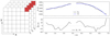 |
Fig. 3. Sketch of the detrending process. A series of consecutive vector magnetograms (e.g., the Bz component) labeled with different time-steps (t1, t2, t3, ...), is shown on the left. The black line (data) in the top right panel represents the temporal evolution of one pixel in this time-series (marked in red in the left panel). The blue line is a third-order polynomial fit to the data. Bottom right panel: detrended time-series, which shows the residuals of the data with respect to the fit. |
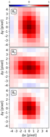 |
Fig. 4. Average spatial correlation of the detrended time-series of a pixel within the leading sunspot of active region NOAA 11072 (2010.05.25 03:00:00−2010.05.25 9:38:00 TAI) relative to its neighbors for the magnetic field vector components Bx, By, and Bz. |
In Appendix B, we consider whether the observed correlations were due to the Postel projection, the detrending method, the 12 and 24 h periodicity of HMI caused by the satellites changing radial velocity relative to the Sun (Hoeksema et al. 2014), or HMI’s point spread function (PSF). We concluded that these correlations are caused by the PSF and the dynamic changes of the magnetic field over time.
We incorporated the information about these time variations of the magnetic field into our model. Knowing that adjacent pixels are correlated but the strength of correlation depends on their position within the spot, we calculated the covariance matrix for all detrended time-series and for each vector component individually. We used the Cholesky decomposition (Haddad 2009) of these covariance matrices to create random correlated maps that reflect spatially correlated temporal fluctuations of the magnetic field. Figure 5 shows example realizations of such maps for each vector component.
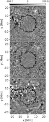 |
Fig. 5. Each panel represents one realization of magnetic field fluctuations for each vector component. All panels are plotted on the same scale in units of Gauss displayed by the color bar at the top. The black solid line represents the observed sunspot boundary. |
4. A model for the reference sunspot
In this section we present the semi-empirical sunspot model developed by (Cameron et al. 2011) modified to represent a uniformly twisted field structure. Cameron et al. (2011) describes a three-dimensional magnetic field model of an axisymmetric sunspot with a radial Br and vertical Bz component. It lacks the azimuthal component Bθ, which is essential for creating twist. We added a Bθ component that is only dependent on the radius without violating the requirement of ∇ ⋅ B = 0 in 3D space. We were only interested in the magnetic field structure on the photospheric level (z = 0) to model a sunspot observed by SDO/HMI. Specifically, the magnetic field at the photosphere is
![$$ \begin{aligned}&B_z(r) = B_0 \exp \left[-\left(\log _{\rm e}2\right)\left(\frac{r}{h_0}\right)^2\right], \end{aligned} $$](/articles/aa/full_html/2022/08/aa43357-22/aa43357-22-eq2.gif)
where B0 is the magnetic field strength at the center of the spot, r is the distance from that center, and h0 defines the radius of the umbra–penumbra boundary. The parameter a0 controls the inclination of the field and b governs the amount of twist in the model. The model of Cameron et al. (2011) is designed so that the inclination of the magnetic field at the umbra–penumbra boundary is 45°. Due to the additional azimuthal component Bθ and to keep the same inclination profile we adjusted the parameter controlling the inclination a0 in accordance with the injected twist by multiplying it with  .
.
The pixel scale of our model is the same as HMI’s pixel scale of 0.5″, which corresponds to approximately 0.35 Mm at disk center. We fit the four free parameters (B0, h0, a0, b) to the reference spot. We use a least-squares fitting approach to best match the azimuthal averages of Bz, Br, and Bθ around the flux-weighted center of the reference sunspots |Bz|.
The information about the twist of the spot is stored in Bθ. As shown in Figs. 1 and 2, Bθ does not show an symmetric behavior about the center of the spot and azimuthal averages do not represent the local twist present in the observation. We find that fitting only the positive or negative values of Bθ yields values of 0.125 and −0.175 for the parameter b, respectively. As the magnetic field twist of the reference sunspot has a preference to be negative, we chose b = −0.15.
The parameters that we find to best describe the reference sunspot with uniform twist are B0 = 2370 G, h0 = 5.2 Mm, a0 = 0.77 Mm, and b = −0.15.
5. Summary and implementation of twist measurement methods
Now we present various methods proposed in the literature to estimate the twist density directly from a single photospheric observation and describe their numerical implementation.
5.1. The twist proxy α
The force-free parameter α can serve as a helicity proxy (Pevtsov et al. 2014) to estimate the twist in uniformly twisted flux tubes (see Appendix F for an interpretation of α in terms of twist). We lack information in photospheric observations of how the Bx and By components of the magnetic field change as a function of height (z-direction in a local Cartesian coordinate system) and we can only compute the vertical current density Jz (e.g., Pevtsov et al. 1994; Longcope et al. 1998).
This vertical current density can be calculated from the force-free equation,
with
Consequently we can compute the local twist proxy αz at a specific location with

We note that α is a pseudo-scalar and the subscript z denotes that it was derived only from the vertical field component and vertical current density. Positive (negative) values of αz correspond to right-handed (left-handed) magnetic field twist, respectively.
Numerically, we calculated the derivatives using the Savitzky-Golay filter (Savitzky & Golay 1964, Appendix C) of cubic and quartic order and a stencil size of five pixels. We note that Jz can also be calculated in integral form using Stokes’ theorem (see Appendix D). The stencil size was chosen based on our own tests on how the stencil size impacts spacial averages of αz (see Appendix E) and the results by Fursyak (2018).
5.2. Average twist
Pevtsov et al. (1995) used a single best fit value of α from linear force-free field extrapolations to characterize the twist for whole active regions. Longcope et al. (1998) used an average ⟨αz⟩ for entire active regions, which can be calculated from photospheric observations without the need of any extrapolations:
Hagino & Sakurai (2004) proposed two weighted averages of αz over a whole active region or spot to determine its twist:
![$$ \begin{aligned} \alpha _{\mathrm{av} }^\mathrm{abs} = \frac{\sum J_z\;\mathrm{sign}\left[B_z\right]}{\sum \left|B_z\right|} \end{aligned} $$](/articles/aa/full_html/2022/08/aa43357-22/aa43357-22-eq10.gif)
and
 and
and  are weighted by absolute and squared Bz, respectively, which is represented by the superscripts “abs” and “sqr”. These latter authors argue that these weighted averages have the advantage of putting less weight on weak field, especially close to the polarity inversion line, where singularities of αz are more likely to occur.
The area over which αz is averaged depends on the area of interest that is studied. In Sect. 7 we investigate averages over a small central area of the spot, the umbra, and the whole spot.
5.3. Peak twist
Under the assumption that a spot can be approximated by a monolithic uniformly twisted magnetic flux tube, Leka et al. (2005) show that the αz profile of this field structure has a peak directly at the center of the spot (flux tube axis), which they name αPeak. Based on the flux tube model by Gold & Hoyle (1960), Leka et al. (2005) demonstrate that αPeak directly relates to the constant twist density q of the field’s structure (αPeak = 2q).
In order to calculate αPeak for a single sunspot, we estimated the location of the flux tube axis by computing the flux-weighted center |Bz| of the sunspot. We calculated a map of αz values (Eq. (7)) for each pixel within the spot and boxcar-smoothed this map to 2″ as suggested by Leka et al. (2005). We used the absolute values of this smoothed map to detect the αz-peak closest to the estimated flux tube axis. αPeak is then the signed and smoothed αz value at the location of the peak.
5.4. Twist density
Nandy et al. (2008) proposed to fit the twist density q to quantify the magnetic twist in a single spot. Again, under the assumption that the magnetic field in a sunspot resembles a uniformly twisted flux tube, q can be measured by fitting the slope of the equation

where r is the distance from the flux tube axis, and Bθ and Bz are the magnetic field in azimuthal direction and along the axis of the tube, respectively. The axis of the tube is estimated by calculating the flux-weighted center of |Bz| of the sunspot. We note that Nandy et al. (2008) allowed a nonzero intercept d to occur in their Fig. 2. This violates the assumption of a vertical uniformly twisted flux tube, where the fitted function is expected to go through zero at r = 0, which is equivalent to a vanishing Bθ at the axis of the flux tube. A physical interpretation of this intercept is not clear to us.
This method was carried out in a cylindrical coordinate system (Br, Bθ, Bz, see Appendix A). We fit the ratio Bθ over Bz for each pixel as a function of the distance between the pixel and the estimated flux tube axis r. The resulting slope corresponds to the twist density q. We tested this method by both allowing an intercept and by forcing the fit through the origin (d = 0).
6. Example sunspot model with correlated magnetic field fluctuations compared to HMI observations
In this section we qualitatively compare the magnetic field and its twist between our sunspot model with one realization of magnetic field fluctuations and the SDO/HMI observations of the reference sunspot in active region NOAA 11072.
6.1. The vector magnetic field
Figure 6 shows that visually the model spot with correlated magnetic field fluctuations resembles the HMI observation of the leading sunspot of active region NOAA 11072 (2010.05.25 03:00:00 TAI). It even exhibits a filamentary structure especially noticeable in Bz, which is not present in the model without fluctuations of the magnetic field. The fluctuation maps (Fig. 5) have smoother and weaker fluctuations within the sunspot, and stronger, more chaotic fluctuations in the quiet Sun, as one would expect from the observations.
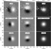 |
Fig. 6. Comparison of the vector components (Bx, By, Bz) of the magnetic field. First row: HMI observation of the leading sunspot of active region NOAA 11072 (2010.05.25 03:00:00 TAI), which serves as the reference for our sunspot model. Second and third rows: model with and without temporal fluctuations, respectively. Every column is plotted on the same scale in units of Gauss displayed by the color bar at the top of the column. |
6.2. The magnetic field’s twist
Figure 7 compares αz-profiles of the original SDO/HMI observation of the reference sunspot and our model with and without one realization of temporal fluctuations of the magnetic field. Our sunspot model without fluctuations describes a uniformly left-handedly twisted magnetic field structure. The αz-profile is azimuthally symmetric and αz increases with distance from the centers of the spots. The sign of αz changes in the penumbra, which signals the presence of return currents (see Appendix F).
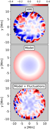 |
Fig. 7. Comparison of αz maps measured from the original HMI observation (top), and from the model without (middle) and with (bottom) fluctuations of the magnetic field. The color bar at the top shows the αz values in Mm−1. |
The reference sunspot has a more complicated structure than the model without temporal fluctuations. Even in the center of the spot, areas of opposite sign of αz exist. Towards the penumbra, positive values of αz become more frequent and one could assume a ring of return currents similar to the model. After applying magnetic field fluctuations to the model, a similar structure of the αz pattern compared to the observations develops.
Our definition of fluctuations includes dynamic variations of the magnetic field. Correlated changes in the direction of magnetic field in adjacent pixels can produce spatially coherent changes in twist and its sign in our model. Sunspot observations typically show a strong radial field component and exhibit only weak twist (i.e. a weak azimuthal field component, Bθ ≪ Br). A source of fluctuations of the magnetic field is the forced environment of the photosphere, where the magnetic field can be buffeted by plasma flows, which can cause sign changes of the real twist. Such an effect is expected to be stronger where the magnetic field strength is weaker – for example in the penumbral parts of the sunspot – where we see the strongest variations of αz within sunspots. Also, interactions with magnetic flux surrounding a sunspot could cause deviations from a uniformly twisted field structure. Complex patterns of αz and magnetic field twist even within the umbra of sunspots have been described in the literature (e.g., Pevtsov et al. 1994; Socas-Navarro 2005; Su et al. 2009).
Figures 8 and 9 show the temporal evolution of αz and its sign for the leading sunspot of active region NOAA 11072, respectively. In Fig. 8 we find that in most parts of the umbra, αz is on the order of 10−2 Mm−1, while penumbral αz values are typically at least one order of magnitude larger, which is consistent with other αz-measurements in sunspots (e.g., Tiwari et al. 2009b; Wang et al. 2021).
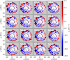 |
Fig. 8. Temporal evolution of αz in the leading sunspot of active region NOAA 11072. The time relative to the first observation (2010.05.25 03:00:00 TAI) is shown in hours in the top left of each panel. The black solid line represents the umbra–penumbra boundary. |
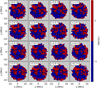 |
Fig. 9. Temporal evolution of the sign of αz in the leading sunspot of active region NOAA 11072. The time relative to the first observation (2010.05.25 03:00:00 TAI) is shown in hours in the top left of each panel. The black solid line represents the umbra–penumbra boundary. |
We find patches of αz with opposite signs throughout the reference sunspot, which is consistent with previous studies of sunspots (e.g., Pevtsov et al. 1994; Socas-Navarro 2005; Su et al. 2009). The shape of these patches are in agreement with findings by Su et al. (2009), who describe a mesh-like pattern in the umbra and a thread-like pattern in the penumbra. Figure 9 shows that many of these patches persist over timescales of hours.
We find a similar distribution of αz values and patterns in the sunspot model with a realization of magnetic field fluctuations. The uncertainty on the mean αz (standard deviation of αz divided by the number of pixels considered) within the model sunspot with fluctuations is of the order of 10−3 Mm−1. This is of the same order as the uncertainty Leka & Skumanich (1999) and Leka (1999) measured in active regions observed with the Image Vector Magnetograph at Mees Solar Observatory.
Features in the pattern structure appear to be on a smaller scale in our model. Pevtsov et al. (1994) studied the helical structure of the magnetic field of three active regions and estimated that the lifetime of such patches can exceed a day. Our model only describes the spatial correlation of magnetic field fluctuations but does not address their temporal correlation. Therefore, these patches appear uncorrelated from one realization to another. Whether or not the temporal variations of the magnetic field are responsible for the twist and current patterns that we can observe in real sunspots cannot be deciphered yet from our model. To further investigate this question, one also has to consider the temporal correlation of the magnetic fluctuations.
7. Sensitivity of twist measurements to correlated temporal fluctuations of the magnetic field
We used Monte-Carlo simulations to test the sensitivity of twist measurement methods described in Sect. 5 to fluctuations of the magnetic field. We used our magnetic field fluctuation model (described in Sect. 3) in 10 000 realisations to create different fluctuation maps and superimposed them on the sunspot model (Sect. 4). We evaluated in each iteration the different twist proxies in the umbra (up to r = h0). We also tested the robustness of the twist measurement methods based on the area over which they are averaged. We evaluated αav in a small umbral area with a radius of 1.75 Mm from the center of the spot ( , white circle in Fig. 10) and up to the penumbra–quiet Sun boundary (
 , black dotted circle in Fig. 10, up to r = 2h0). Fluctuations of the magnetic field in our model can result in vertical field Bz close to zero in the penumbra, which can create singularities when calculating αz = Jz/Bz. Therefore, we only measure αz for pixels that are above a Bz threshold of 50 Gauss. The analytically calculated reference values of αz and q that represent the uniform twist of our model best (see Appendix F) are
  Mm−1.
Mm−1.
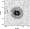 |
Fig. 10. HMI continuum image of the leading sunspot of active region NOAA 11072 (2010.05.25 03:00:00 TAI), which was used as a reference for the model presented in this work. The black solid line outlines the umbral area that was considered for most twist calculation methods. The white solid line and the black dotted line correspond to the areas that were used to get spatial averages of αz close to the center of the spot ( |


Figures 11 and 12 show the distribution of the calculated twist proxies from the Monte-Carlo simulations for each method. Table 1 compares the mean result and standard deviation from the Monte-Carlo simulations against the expected value from the model without fluctuations. It is important to note that the “Model” values in Table 1 are derived when a method is applied in the fluctuation-free model. The errors given in Table 1 show the standard deviation of the Monte-Carlo simulations. We find that the expectation values of the averaging methods and the twist density fits are not biased by magnetic field fluctuations.
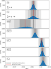 |
Fig. 11. Monte-Carlo simulation results for methods described in Sect. 5. The q values have been multiplied by two in order to make them directly comparable to αz (see Appendix F). The black line indicates the reference value of the model, which is expected from the model without any fluctuations. The red dashed line shows the mean value from the Monte-Carlo simulations. The gray shaded areas represent the range of 1, 2, and 3σ around the Monte-Carlo mean. |
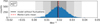 |
Fig. 12. Monte-Carlo simulation results when αz is spatially averaged over the whole sunspot. The solid black line indicates the reference value of the model that is expected from the model without any fluctuations. The red dashed line shows the mean value from the Monte-Carlo simulations. The gray shaded areas represent the range of 1, 2, and 3σ around the mean. |
Comparison of the different twist calculation methods between the model reference without any fluctuations of the magnetic field (Model) and the Monte-Carlo simulations (MC Sim.).
The averaging methods of αz show a large spread in their results, but have robust measurements under magnetic field fluctuations. These different spatial averages of αz can still be related to the twist density based on the azimuthal symmetric behavior of αz in our simple model. We derive ![$ \alpha_z (r) = 2q\left[1-\left(\log_{\mathrm{e}}2\right)\left(\frac{r}{h_0}\right)^2\right] $](/articles/aa/full_html/2022/08/aa43357-22/aa43357-22-eq26.gif) in Appendix F. We can calculate the average value of αz in a circular area with radius r around the center of the spot:
in Appendix F. We can calculate the average value of αz in a circular area with radius r around the center of the spot:
![$$ \begin{aligned} \begin{aligned} \langle \alpha _z \rangle _{\rm r} = \frac{1}{\pi r^2} \int _0^r \int _0^{2\pi } \alpha _z (\tilde{r})\ \tilde{r}\mathrm{d}\tilde{r}\mathrm{d}\theta = \left[2-\left(\log _{\rm e}2\right) \left(\frac{r}{h_0}\right)^2\right]q. \end{aligned} \end{aligned} $$](/articles/aa/full_html/2022/08/aa43357-22/aa43357-22-eq27.gif)
Consequently, we find the following relation between the twist density q and ⟨αz⟩r:
This equation is consistent with the relation of αPeak = 2q at the center of the spot. It also describes the different spatial averages of αz that we measure, when the averaging radius was changed (see Figs. 11 and 12). We measure a larger ⟨αz⟩ when averaged over a small area at the center of the spot ( ) compared to the average over the umbra (αav). When the averaging radius becomes sufficiently large (e.g.,
  ), ⟨αz⟩ retrieves the opposite sign compared to αz in the center of the spot.
The expectation value of the αPeak method is noticeably biased, causing an overestimation of the twist density in the presence of magnetic field fluctuations. As this method characterizes the twist density with a single peak value closest to the center of the spot, it is likely to pick up any enhanced signal caused by the fluctuations of the magnetic field.
The twist density fit (Nandy et al. 2008) retrieves the analytical twist density value. We find a larger spread in the resulting values when no zero-intercept is forced. These results are expected, because the equations of our sunspot model can be exactly reduced to the fitting equation by Nandy et al. (2008). Crouch (2012) shows that fitting techniques can be sensitive to small discrepancies between the fitting and reference model. Observations suggest that sunspots are more complicated and can have nonuniformly twisted field structures (e.g., Socas-Navarro 2005; Su et al. 2009). Another complication for real sunspots is that this method requires the exact location of the axis of a flux tube as a center for the coordinate transformation to cylindrical coordinates. This is a simple task in our model without fluctuations, because the central axis of the model spot and its flux-weighted center fall into the same place by definition; even with magnetic field fluctuations, they are always located close to each other. In real sunspots, the axis of the spot does not have to be in the same place as its flux-weighted center. Also, a sunspot may not have an underlying uniformly twisted vertical field structure.
In Sect. 4 we chose the model parameter b = −0.15, which governs the twist in our model. We tested various values of b, ranging from untwisted field (b = 0) to highly twisted field (b = 10) and found that the amount of twist in the model does not influence the findings about the robustness of the twist measurements described in this section.
8. Summary and conclusion
We derived a model for the spatially correlated fluctuations of the magnetic field in a sunspot based on HMI observations of the leading sunspot of the active region NOAA 11072. We superposed realizations of the fluctuations on the magnetic field of the semi-empirical sunspot model described in Cameron et al. (2011) with added uniform twist. We carried out Monte-Carlo simulations to test the robustness of the different measures of the twist to the fluctuations.
We considered measurement methods based on estimating either the force-free parameter αz or the twist density of the magnetic field q. In the absence of fluctuations, and for the sunspot model used in this paper, the value of αz at the center of the sunspot is twice the twist parameter q (see Leka et al. 2005). For our chosen twist profile, αz is not uniform and changes sign in the penumbra of the model spot.
Including the spatially correlated temporal fluctuations of the magnetic field qualitatively reproduces features seen in vertical current density Jz and αz observations. Patches with opposite sign of αz appear throughout the sunspot model at random locations from one realization to another. Although we do not consider temporal correlations of the fluctuations, we note that such features can persist for hours in observations (Pevtsov et al. 1994).
All measures except αPeak have expectation values consistent with that of the model without fluctuations. The fluctuations do not introduce a bias. The measures based on spatial averages of αz have different expectation values, because they average over different portions of the nonuniform αz profile. Due to the sign change of αz in the penumbra of our model, any spatial averages of αz that reach too far out from the center of the spot can have the opposite sign from αz near the center of the spot. The expectation value of αPeak is biased with respect to the model without fluctuations. The magnitude of the bias is related to the level of the magnetic field fluctuations.
For most methods, the spread of results from the Monte-Carlo simulations is less than the spread in expectation values of the individual methods. Therefore, the choice of method is more significant than the impact of the magnetic field fluctuations on the measurements.
Our results are for the particular sunspot model given by Eqs. (2)–(4). This is a particularly simple axisymmetric sunspot model. For sunspots with a more complex structure, for example nonuniformly twisted sunspots, the applicability and meaning of the different measures needs to be carefully considered (e.g., Crouch 2012). In this regard, we note that the SDO/HMI observations of the leading spot of active region NOAA 11072 had fine structure in αz which persisted for longer than 7 h. This persistent fine structure suggests a more complicated underlying field structure than that of our uniformly twisted model. The long-lived fine structure found in active region NOAA 11072 is consistent with previous studies of other sunspots (e.g., Pevtsov et al. 1994; Su et al. 2009).
As was previously noted by Leka (1999), a single parameter will not in general characterize the twist of a sunspot. In this paper, we show that a range of different complementary parameters exists, all of which describe somewhat different aspects of the magnetic field line twist in sunspots. We show that most of these measures are robust to fluctuations of the field.
Acknowledgments
C.B. is a member of the International Max Planck Research School (IMPRS) for Solar System Science at the University of Göttingen. C.B. conducted the analysis, contributed to the interpretation of the results, and wrote the manuscript. We thank Jesper Schou for helpful discussions. We thank Graham Barnes for useful comments on the manuscript. The HMI data used are courtesy of NASA/SDO and the HMI Science Team. A.C.B., R.H.C. and L.G. acknowledge partial support from the European Research Council Synergy Grant WHOLE SUN #810218. The data were processed at the German Data Center for SDO, funded by the German Aerospace Center under grant DLR50OL1701. This research made use of the Astropy (Astropy Collaboration 2013, 2018), Matplotlib (Hunter 2007), NumPy (Van Der Walt et al. 2011) and SciPy (Virtanen et al. 2020) Python packages.
References
- Astropy Collaboration (Robitaille, T. P., et al.) 2013, A&A, 558, A33 [NASA ADS] [CrossRef] [EDP Sciences] [Google Scholar]
- Astropy Collaboration (Price-Whelan, A. M., et al.) 2018, AJ, 156, 123 [Google Scholar]
- Berger, M., & Field, G. 1984, J. Fluid Mech., 147, 133 [NASA ADS] [CrossRef] [Google Scholar]
- Borrero, J. M., & Ichimoto, K. 2011, Liv. Rev. Sol. Phys., 8, 4 [Google Scholar]
- Brandenburg, A. 2005, ApJ, 625, 539 [NASA ADS] [CrossRef] [Google Scholar]
- Burnette, A. B., Canfield, R. C., & Pevtsov, A. A. 2004, ApJ, 606, 565 [NASA ADS] [CrossRef] [Google Scholar]
- Cameron, R. H., Gizon, L., Schunker, H., & Pietarila, A. 2011, Sol. Phys., 268, 293 [NASA ADS] [CrossRef] [Google Scholar]
- Charbonneau, P. 2020, Liv. Rev. Sol. Phys., 17, 4 [Google Scholar]
- Crouch, A. D. 2012, Sol. Phys., 281, 669 [NASA ADS] [CrossRef] [Google Scholar]
- Fan, Y. 2005, ApJ, 630, 543 [NASA ADS] [CrossRef] [Google Scholar]
- Fan, Y., & Gibson, S. E. 2004, ApJ, 609, 1123 [NASA ADS] [CrossRef] [Google Scholar]
- Fursyak, Y. A. 2018, Geomagn. Aeron., 58, 1129 [NASA ADS] [CrossRef] [Google Scholar]
- Gary, G. A. 2001, Sol. Phys., 203, 71 [Google Scholar]
- Gary, G. A., & Hagyard, M. J. 1990, Sol. Phys., 126, 21 [Google Scholar]
- Gilman, P. A., & Charbonneau, P. 1999, Washington DC American Geophysical Union Geophysical Monograph Series, 111, 75 [NASA ADS] [Google Scholar]
- Gold, T., & Hoyle, F. 1960, MNRAS, 120, 89 [NASA ADS] [Google Scholar]
- Haddad, C. N. 2009, Encyclopedia of Optimization (Boston, MA: Springer US), 374 [CrossRef] [Google Scholar]
- Hagino, M., & Sakurai, T. 2004, PASJ, 56, 831 [NASA ADS] [CrossRef] [Google Scholar]
- Hoeksema, J. T., Liu, Y., Hayashi, K., et al. 2014, Sol. Phys., 289, 3483 [Google Scholar]
- Hunter, J. D. 2007, Comput. Sci. Eng., 9, 90 [NASA ADS] [CrossRef] [Google Scholar]
- Leka, K. D. 1999, Sol. Phys., 188, 21 [NASA ADS] [CrossRef] [Google Scholar]
- Leka, K. D., & Skumanich, A. 1999, Sol. Phys., 188, 3 [NASA ADS] [CrossRef] [Google Scholar]
- Leka, K. D., Fan, Y., & Barnes, G. 2005, ApJ, 626, 1091 [NASA ADS] [CrossRef] [Google Scholar]
- Longcope, D. W., Fisher, G. H., & Pevtsov, A. A. 1998, ApJ, 507, 417 [NASA ADS] [CrossRef] [Google Scholar]
- Nandy, D. 2006, J. Geophys. Res.: Space Phys., 111, A12S01 [NASA ADS] [CrossRef] [Google Scholar]
- Nandy, D., Mackay, D. H., Canfield, R. C., & Martens, P. C. H. 2008, J. Atmos. Sol.-Terr. Phys., 70, 605 [NASA ADS] [CrossRef] [Google Scholar]
- Pevtsov, A. A., Canfield, R. C., & Metcalf, T. R. 1994, ApJ, 425, L117 [NASA ADS] [CrossRef] [Google Scholar]
- Pevtsov, A. A., Canfield, R. C., & Metcalf, T. R. 1995, ApJ, 440, L109 [NASA ADS] [CrossRef] [Google Scholar]
- Pevtsov, A. A., Berger, M. A., Nindos, A., Norton, A. A., & van Driel-Gesztelyi, L. 2014, Space Sci. Rev., 186, 285 [NASA ADS] [CrossRef] [Google Scholar]
- Pipin, V. V., Zhang, H., Sokoloff, D. D., Kuzanyan, K. M., & Gao, Y. 2013, MNRAS, 435, 2581 [NASA ADS] [CrossRef] [Google Scholar]
- Savitzky, A., & Golay, M. J. E. 1964, Anal. Chem., 36, 1627 [Google Scholar]
- Seehafer, N. 1990, Sol. Phys., 125, 219 [NASA ADS] [CrossRef] [Google Scholar]
- Socas-Navarro, H. 2005, ApJ, 631, L167 [NASA ADS] [CrossRef] [Google Scholar]
- Su, J. T., Sakurai, T., Suematsu, Y., Hagino, M., & Liu, Y. 2009, ApJ, 697, L103 [NASA ADS] [CrossRef] [Google Scholar]
- Tiwari, S. K., Venkatakrishnan, P., Gosain, S., & Joshi, J. 2009a, ApJ, 700, 199 [NASA ADS] [CrossRef] [Google Scholar]
- Tiwari, S. K., Venkatakrishnan, P., & Sankarasubramanian, K. 2009b, ApJ, 702, L133 [NASA ADS] [CrossRef] [Google Scholar]
- Török, T., & Kliem, B. 2003, A&A, 406, 1043 [NASA ADS] [CrossRef] [EDP Sciences] [Google Scholar]
- Török, T., Kliem, B., & Titov, V. S. 2004, A&A, 413, L27 [NASA ADS] [CrossRef] [EDP Sciences] [Google Scholar]
- Van Der Walt, S., Colbert, S. C., & Varoquaux, G. 2011, Comput. Sci. Eng., 13, 22 [Google Scholar]
- Virtanen, P., Gommers, R., Oliphant, T. E., et al. 2020, Nat. Meth., 17, 261 [Google Scholar]
- Wang, J., Yan, X., Kong, D., et al. 2021, A&A, 652, A55 [NASA ADS] [CrossRef] [EDP Sciences] [Google Scholar]
- Wiegelmann, T., & Sakurai, T. 2012, Liv. Rev. Sol. Phys., 9, 5 [Google Scholar]
- Woltjer, L. 1958, Proc. Natl. Acad. Sci., 44, 489 [NASA ADS] [CrossRef] [Google Scholar]
- Yeates, A. R., Mackay, D. H., & van Ballegooijen, A. A. 2008, Sol. Phys., 247, 103 [NASA ADS] [CrossRef] [Google Scholar]
- Yeo, K. L., Feller, A., Solanki, S. K., et al. 2014, A&A, 561, A22 [NASA ADS] [CrossRef] [EDP Sciences] [Google Scholar]
Appendix A: Vector transformation
A.1. Local Cartesian coordinates
The hmi.b_720s (Hoeksema et al. 2014) provides the vector magnetic field in spherical coordinates aligned with the line of sight (LoS); it includes the absolute field strength B, the inclination angle “inc” with respect to the LoS, and the azimuth angle “azi” (whose ambiguity has to be resolved) measured in a plane perpendicular to the LoS. We study the magnetic field in a local Cartesian and cylindrical coordinate system, where Bz is pointing radially outwards from the Sun. In order to transform the spherical coordinate system to a local Cartesian coordinate system, we followed the transformations described in Gary & Hagyard (1990).
First, the spherical vector components were transformed to a Cartesian system, where Bζ is aligned with the LoS, while Bξ and Bη lay in the plane perpendicular to the LoS:
We then rotated the coordinate system (Eq. A.4) so that Bζ points radially outward from the Sun and becomes Bz. Here, Bx and By point from solar east to west and south to north, respectively. The rotation matrix is
with the transformation matrix coefficients aij:
![$$ \begin{aligned} a_{11} =&- \sin B_0\sin P\sin (L-L_0)+\cos P\cos (L-L_0) \\ a_{12} =&+ \sin B_0 \cos P \sin (L-L_0) + \sin P \cos (L-L_0) \\ a_{13} =&- \cos B_0 \sin (L-L_0) \\ a_{21} =&- \sin B \left[ \sin B_0 \sin P \cos (L-L_0) + \cos P \sin (L-L_0) \right] \\&- \cos B \left[ \cos B_0 \sin P \right]\\ a_{22} =&+ \sin B \left[ \sin B_0 \cos P \cos (L-L_0) - \sin P \sin (L-L_0) \right] \\ a_{23} =&- \cos B_0 \sin B \cos (L-L_0) + \sin B_0 \cos B\\ a_{31} =&+ \cos B \left[ \sin B_0 \sin P \cos (L-L_0) + \cos P \sin (L-L_0) \right] \\&- \sin B \left[ \cos B_0 \sin P \right] \\&+ \cos B \left[ \cos B_0 \cos P \right] \\ a_{32} =&- \cos B \left[ \sin B_0 \cos P \cos (L-L_0) + \sin P \sin (L-L_0) \right] \\&+ \sin B \left[ \cos B_0 \cos P \right] \\ a_{33} =&+ \cos B \cos B_0 \cos (L-L_0) + \sin B \sin B_0. \end{aligned} $$](/articles/aa/full_html/2022/08/aa43357-22/aa43357-22-eq35.gif)
Here, L and B describe the heliographic longitude and latitude of the individual pixels, while L0 and B0 are the longitude and latitude of the solar disk center, respectively, and P is the solar position angle.
A.2. Cylindrical coordinates
We transformed from the local Cartesian coordinate system to a local cylindrical coordinate system by calculating
with θ = arctan2(y, x). The flux-weighted center of a spot is defined as the origin (x = 0, y = 0) for this transformation. In this coordinate system, Bz is the component normal to the surface; Br and Bθ are located in a plane parallel to the surface; Br points radially away from the center of the spot; and Bθ is always perpendicular to Br and Bz.
Appendix B: Possible causes for the measured spatial correlation of magnetic field fluctuations
We tested various effects that could introduce the spatial correlation of temporal fluctuations of neighboring pixels. To assess the effect of the Postel projections on these correlations, we created artificial full-disk HMI maps. We filled pixels with random Gaussian white noise with a mean of zero and standard deviation of one. We created Postel-projected time-series of submaps at different locations on the solar disk based on the center to limb angle (CTL) of the center of the submap. We followed the same detrending procedure as described in section 3, but find no correlation of adjacent pixels either at disk center (CTL = 0°) or close to the limb (CTL = 60°).
We compared different ways of detrending the data: different order of polynomials for fitting (order 3, 4, and 5), differences to previous data points, and running averages. All different detrending methods show similar correlations of adjacent pixels. We find no relation of the detrended signals to the known 12- and 24-hour period systematic errors of HMI that are caused by the satellite’s orbit and change in radial velocity relative to the Sun.
The PSF of HMI definitely contributes to the correlations of adjacent pixels. Figure B.1 shows an estimate of the PSF of HMI by Yeo et al. (2014). Figure B.2 shows cuts along the x- and y-axis through the center of the normalized PSF, and the average correlations of adjacent pixels are shown in Fig. 4. We find that the fluctuations of the vector magnetic field components are correlated up to spatial scales that are 30% larger than that expected from the HMI PSF. We suggest that these correlations are caused by the PSF and the dynamic changes of the magnetic field over time with respect to the underlying global field structure of the sunspot.
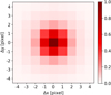 |
Fig. B.1. Normalized PSF for HMI estimated by Yeo et al. (2014). |
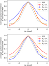 |
Fig. B.2. Cuts through the center along the x-axis (top panel) and the y-axis (bottom panel) of the average spatial correlation of neighboring pixels (Fig. 4) and the normalized estimated PSF by Yeo et al. (2014) (Fig. B.1). The errorbars represent the standard error of the spatially averaged correlation. |
Appendix C: Derivatives with different stencil sizes
We can evaluate derivatives with different stencil sizes using Savitzky-Golay filter (Savitzky & Golay 1964) of cubic/quartic order for stencil sizes of 5 and 7 pixels or take a central differences approach for a stencil of 3 pixels:
where x describes the location of a pixel counted as integer, for which we want to calculate the derivative. S is the stencil size, N is a normalization factor, h is the pixel scale, and g is a weighting factor. The weighting and normalization factor for the different stencil sizes are listed in Table C.1.
Weighting factors g(i) and normalization factors N for stencil sizes S of 7, 5, and 3 pixels for Eq. C.1.
Appendix D: Using Stokes’ theorem for calculating Jz
Instead of using derivatives for calculating Jz (Eq. 6), one can also use Stokes’ theorem:
where the vertical current density is calculated for a pixel in the center of an area AL outlined by a contour L. We calculated the integral by using the composite Simpson’s rule over a square, where L is the edge of the square with a side length of 3, 5, or 7 pixels, in accordance to the stencil size when using derivatives.
Using Stokes’ theorem for calculating αz leads on average to slightly lower values compared to the differential form. This effect can be attributed to the integral form using more pixels for the calculations and averaging over an area. The results of Monte-Carlo simulations are shown in Fig. D.1 and Fig. D.2 as well as Table D.1.
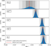 |
Fig. D.1. Monte-Carlo simulation results for methods based on αz when Stokes’ theorem is used for calculating Jz. The black solid line indicates the reference value of the model that is expected from the model without any fluctuations. The red dashed line shows the mean value from the Monte-Carlo simulations. The dark/light gray shaded areas represent the range of 1, 2, or 3σ around the Monte-Carlo mean. |
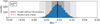 |
Fig. D.2. Monte-Carlo simulation results when αz is calculated with Stokes’ theorem and spatially averaged over the whole sunspot. The black solid line indicates the reference value of the model that is expected from the model without any fluctuations. The red dashed line shows the mean value from the Monte-Carlo simulations. The gray shaded areas represent the range of 1, 2, and 3σ around the mean. |
Comparison of the different twist calculation methods between the model reference without any fluctuations of the magnetic field (Model) and the Monte-Carlo simulations (MC Sim.). All parameters were calculated using Stokes’ theorem. Values are given in Mm−1.
Appendix E: Comparison of different stencil sizes for calculating Jz
We tested stencil sizes of 3, 5, and 7 pixels in Monte-Carlos simulations as described in section 7 to determine how many pixels should be considered for calculating the vertical current density Jz and subsequently αz. The average twist proxy values and their standard deviation from these simulations are listed in Tables E.1 and E.2. The different stencil sizes do not noticeably impact the end result when we used the Savitzky-Golay filter. In contrast, we find that with bigger areas the measured twist goes down when Stokes’ theorem (see Appendix D) was applied. Similar to the Monte-Carlo simulations described in section 7 only the expectation value of the αPeak method is biased in all test cases.
Monte-Carlo simulation results for using derivatives to calculate αz with stencil sizes of 3, 5, and 7 pixels, when αz was evaluated in the umbra of the model spot.
Monte-Carlo simulation results for using integration to calculate αz over square areas with side lengths of 3, 5, and 7 pixels, when αz was evaluated in the model spot’s umbra.
Fursyak (2018) tested the effect of differently sized areas for calculating Jz in differential and integral forms using observations from Hinode and HMI. They conclude that integrating over side lengths of five pixels provides the best compromise between smoothing noise but still preserving significant features. As the results from our tests do not show a clear favorite, we chose to calculate Jz with stencil sizes of 5 pixels in accordance to Fursyak (2018).
Appendix F: Interpretation of αz
It is often difficult to interpret αz measurements. Ideally we would expect to measure the same αz or twist density q value at each location within a uniformly twisted flux tube (which is the case in thin flux tube models). While this is true for the twist density q in our sunspot model without magnetic field fluctuations, αz varies with the distance from the center of the spot, where the αz profile peaks.
Leka et al. (2005) used the Gold-Hoyle flux tube model (Gold & Hoyle 1960) to show the connection between αz and the twist density. This model consists of an axial and azimuthal magnetic field component. Leka et al. (2005) demonstrate that only at the center of the flux tube, where the radial distance from its axis r equals zero, the twist density can be retrieved from αz measurements directly. They describe the following relationship between αz, the twist density q and the distance from the flux tube axis as:
We note that in this configuration αz goes towards zero when r increases to infinity. This finding led them to propose the αPeak method. We can find a similar relationship between αPeak and the twist density q for our empirical sunspot model. Taking the model’s equation for Bθ (Eq. 4) with  , we get the twist density equation from Nandy et al. (2008):

Together with the model’s Bz component,
![$$ \begin{aligned} B_z(r) = B_0 \exp \left[-\left(\log _{\rm e}2\right)\left(\frac{r}{h_0}\right)^2\right], \end{aligned} $$](/articles/aa/full_html/2022/08/aa43357-22/aa43357-22-eq50.gif)
we can use derivatives in cylindrical coordinates to calculate αz. We note that Br in Eq. 3 does not depend on the azimuthal angle θ. Then the radial profile of αz is:
![$$ \begin{aligned} \alpha _z&= \frac{1}{r B_z} \left[\frac{\partial (r B_\theta )}{\partial r} - {\frac{\partial B_r}{\partial \theta }}\right]\nonumber \\&= \frac{1}{r B_z} \frac{\partial }{\partial r} \left\{ q B_0 r^2 \exp \left[-\left(\log _{\rm e}2\right)\left(\frac{r}{h_0}\right)^2\right]\right\} \nonumber \\&= 2 q \left[1 - \left(\log _{\rm e}2\right)\left(\frac{r}{h_0}\right)^2\right]. \end{aligned} $$](/articles/aa/full_html/2022/08/aa43357-22/aa43357-22-eq51.gif)
We get a maximum value of αz (αPeak) at the center of the flux tube, i.e. r = 0. Therefore, we find the same relationship of αPeak = 2q as Leka et al. (2005).
In our empirical sunspot model αz changes sign at a certain distance from the suncenter of the spot. We can determine where alpha changes sign by setting αz in Eq. F.4 equal to zero to get
The parameter h0 describes the distance of the umbra–penumbra boundary measured from the model center of the spot. Disregarding fluctuations of the magnetic field, within the umbra the sign of the twist and αz are the same, according to our model.
Since αz = Jz/Bz, such a sign reversal can only happen in our sunspot model with positive polarity, if the sign of the vertical current density Jz changes. Such rings of return currents at the umbra–penumbra boundary of observed sunspots are reported in literature (e.g., Tiwari et al. 2009b). We note that positive and negative vertical currents are balanced in our model.
All Tables
Comparison of the different twist calculation methods between the model reference without any fluctuations of the magnetic field (Model) and the Monte-Carlo simulations (MC Sim.).
Weighting factors g(i) and normalization factors N for stencil sizes S of 7, 5, and 3 pixels for Eq. C.1.
Comparison of the different twist calculation methods between the model reference without any fluctuations of the magnetic field (Model) and the Monte-Carlo simulations (MC Sim.). All parameters were calculated using Stokes’ theorem. Values are given in Mm−1.
Monte-Carlo simulation results for using derivatives to calculate αz with stencil sizes of 3, 5, and 7 pixels, when αz was evaluated in the umbra of the model spot.
Monte-Carlo simulation results for using integration to calculate αz over square areas with side lengths of 3, 5, and 7 pixels, when αz was evaluated in the model spot’s umbra.
All Figures
|
Fig. 1. SDO/HMI vector magnetogram of the leading sunspot of active region NOAA 11072 (2010.05.25 03:00:00 TAI) in cylindrical coordinates. Br (top), Bθ (middle), and Bz (bottom) show the radial, azimuthal, and vertical component of the magnetic field. |
| In the text | |
|
Fig. 2. SDO/HMI vector magnetogram of the leading sunspot of active region NOAA 11072 (2010.05.25 03:00:00 TAI) with the horizontal field Bhor plotted as arrows on top of the vertical vector component Bz. |
| In the text | |
|
Fig. 3. Sketch of the detrending process. A series of consecutive vector magnetograms (e.g., the Bz component) labeled with different time-steps (t1, t2, t3, ...), is shown on the left. The black line (data) in the top right panel represents the temporal evolution of one pixel in this time-series (marked in red in the left panel). The blue line is a third-order polynomial fit to the data. Bottom right panel: detrended time-series, which shows the residuals of the data with respect to the fit. |
| In the text | |
|
Fig. 4. Average spatial correlation of the detrended time-series of a pixel within the leading sunspot of active region NOAA 11072 (2010.05.25 03:00:00−2010.05.25 9:38:00 TAI) relative to its neighbors for the magnetic field vector components Bx, By, and Bz. |
| In the text | |
|
Fig. 5. Each panel represents one realization of magnetic field fluctuations for each vector component. All panels are plotted on the same scale in units of Gauss displayed by the color bar at the top. The black solid line represents the observed sunspot boundary. |
| In the text | |
|
Fig. 6. Comparison of the vector components (Bx, By, Bz) of the magnetic field. First row: HMI observation of the leading sunspot of active region NOAA 11072 (2010.05.25 03:00:00 TAI), which serves as the reference for our sunspot model. Second and third rows: model with and without temporal fluctuations, respectively. Every column is plotted on the same scale in units of Gauss displayed by the color bar at the top of the column. |
| In the text | |
|
Fig. 7. Comparison of αz maps measured from the original HMI observation (top), and from the model without (middle) and with (bottom) fluctuations of the magnetic field. The color bar at the top shows the αz values in Mm−1. |
| In the text | |
|
Fig. 8. Temporal evolution of αz in the leading sunspot of active region NOAA 11072. The time relative to the first observation (2010.05.25 03:00:00 TAI) is shown in hours in the top left of each panel. The black solid line represents the umbra–penumbra boundary. |
| In the text | |
|
Fig. 9. Temporal evolution of the sign of αz in the leading sunspot of active region NOAA 11072. The time relative to the first observation (2010.05.25 03:00:00 TAI) is shown in hours in the top left of each panel. The black solid line represents the umbra–penumbra boundary. |
| In the text | |
|
Fig. 10. HMI continuum image of the leading sunspot of active region NOAA 11072 (2010.05.25 03:00:00 TAI), which was used as a reference for the model presented in this work. The black solid line outlines the umbral area that was considered for most twist calculation methods. The white solid line and the black dotted line correspond to the areas that were used to get spatial averages of αz close to the center of the spot ( |
| In the text | |
|
Fig. 11. Monte-Carlo simulation results for methods described in Sect. 5. The q values have been multiplied by two in order to make them directly comparable to αz (see Appendix F). The black line indicates the reference value of the model, which is expected from the model without any fluctuations. The red dashed line shows the mean value from the Monte-Carlo simulations. The gray shaded areas represent the range of 1, 2, and 3σ around the Monte-Carlo mean. |
| In the text | |
|
Fig. 12. Monte-Carlo simulation results when αz is spatially averaged over the whole sunspot. The solid black line indicates the reference value of the model that is expected from the model without any fluctuations. The red dashed line shows the mean value from the Monte-Carlo simulations. The gray shaded areas represent the range of 1, 2, and 3σ around the mean. |
| In the text | |
|
Fig. B.1. Normalized PSF for HMI estimated by Yeo et al. (2014). |
| In the text | |
|
Fig. B.2. Cuts through the center along the x-axis (top panel) and the y-axis (bottom panel) of the average spatial correlation of neighboring pixels (Fig. 4) and the normalized estimated PSF by Yeo et al. (2014) (Fig. B.1). The errorbars represent the standard error of the spatially averaged correlation. |
| In the text | |
|
Fig. D.1. Monte-Carlo simulation results for methods based on αz when Stokes’ theorem is used for calculating Jz. The black solid line indicates the reference value of the model that is expected from the model without any fluctuations. The red dashed line shows the mean value from the Monte-Carlo simulations. The dark/light gray shaded areas represent the range of 1, 2, or 3σ around the Monte-Carlo mean. |
| In the text | |
|
Fig. D.2. Monte-Carlo simulation results when αz is calculated with Stokes’ theorem and spatially averaged over the whole sunspot. The black solid line indicates the reference value of the model that is expected from the model without any fluctuations. The red dashed line shows the mean value from the Monte-Carlo simulations. The gray shaded areas represent the range of 1, 2, and 3σ around the mean. |
| In the text | |
Current usage metrics show cumulative count of Article Views (full-text article views including HTML views, PDF and ePub downloads, according to the available data) and Abstracts Views on Vision4Press platform.
Data correspond to usage on the plateform after 2015. The current usage metrics is available 48-96 hours after online publication and is updated daily on week days.
Initial download of the metrics may take a while.