| Issue |
A&A
Volume 664, August 2022
|
|
|---|---|---|
| Article Number | A144 | |
| Number of page(s) | 21 | |
| Section | Extragalactic astronomy | |
| DOI | https://doi.org/10.1051/0004-6361/202243028 | |
| Published online | 19 August 2022 | |
Warm ionized gas in the blue compact galaxy Haro 14 viewed by MUSE⋆
The diverse ionization mechanisms acting in low-mass starbursts
1
Institut für Astrophysik, Georg-August-Universität, Friedrich-Hund-Platz 1, 37077 Göttingen, Germany
e-mail: luzma@astro.physik.uni-goettingen.de
2
Hamburger Sternwarte, Gojenbergsweg 112, 21029 Hamburg, Germany
3
Leibniz-Institut für Astrophysik (AIP), An der Sternwarte 16, 14482 Potsdam, Germany
4
Max Planck Institute for Solar System Research, Justus-von-Liebig-Weg 3, 37077 Göttingen, Germany
Received:
1
January
2022
Accepted:
25
April
2022
We investigate the warm ionized gas in the blue compact galaxy (BCG) Haro 14 by means of integral field spectroscopic observations taken with the Multi Unit Spectroscopic Explorer (MUSE) at the Very Large Telescope. The large field of view of MUSE and its unprecedented sensitivity enable observations of the galaxy nebular emission up to large galactocentric distances, even in the important but very faint [O I] λ6300 diagnostic line. This allowed us to trace the ionized gas morphology and ionization structure of Haro 14 up to kiloparsec scales and, for the first time, to accurately investigate the excitation mechanism operating in the outskirts of a typical BCG. The intensity and diagnostic maps reveal at least two highly distinct components of ionized gas: the bright central regions, mostly made of individual clumps, and a faint component which extends up to kiloparsec scales and consists of widespread diffuse emission, well-delineated filamentary structures, and faint knots. Noteworthy are the two curvilinear filaments extending up to 2 and 2.3 kpc southwest, which likely trace the edges of supergiant expanding bubbles driven by galactic outflows. We find that while the central clumps in Haro 14 are H II-region complexes, the morphology and line ratios of the whole low-surface-brightness component are not compatible with star formation photoionization. In the spatially resolved emission-line-ratio diagnostic diagrams, spaxels above the maximum starburst line form the majority (∼75% and ∼50% in the diagnostic diagrams involving [O I] and [S II] respectively). Moreover, our findings suggest that more than one alternative mechanism is ionizing the outer galaxy regions. The properties of the diffuse component are consistent with ionization by diluted radiation and the large filaments and shells are most probably shocked areas at the edge of bubbles. The mechanism responsible for the ionization of the faint individual clumps observed in the galaxy periphery is more difficult to assess. These clumps could be the shocked debris of fragmented shells or regions where star formation is proceeding under extreme conditions.
Key words: galaxies: individual: Haro14 / galaxies: dwarf / galaxies: starburst / galaxies: ISM / galaxies: star formation / galaxies: abundances
© L. M. Cairós et al. 2022
 Open Access article, published by EDP Sciences, under the terms of the Creative Commons Attribution License (https://creativecommons.org/licenses/by/4.0), which permits unrestricted use, distribution, and reproduction in any medium, provided the original work is properly cited.
This article is published in open access under the Subscribe-to-Open model. Subscribe to A&A to support open access publication.
1. Introduction
Blue compact galaxies (BCGs) are low-mass, metal-poor, gas-rich objects that form stars at extremely high rates (Thuan & Martin 1981; Thuan et al. 1999; Cairós et al. 2001; Gil de Paz et al. 2003; Shi et al. 2005). These unusual characteristics mean that they are key targets in extragalactic astronomy. In particular, research into BCGs is fundamental for improving our understanding of large-scale (galactic) star formation (SF) and the impact of massive stellar feedback on galaxy formation and evolution (Marlowe et al. 1995, 1997; Martin 1998; Cairós & González-Pérez 2017a,b, 2020; McQuinn et al. 2018, 2019).
BCGs cannot develop spiral density waves or strong shear forces, and therefore enable us to probe the process of SF in a relatively simple environment (Hunter & Gallagher 1986; Hunter 1997). In addition, while in larger galaxies the collapse of gas clouds is explained (at least in part) as being due to the effect of density waves (Shu et al. 1972; Seigar & James 2002), the mechanism responsible for the SF ignition in low-mass systems is still unclear (Pustilnik et al. 2001; Brosch et al. 2004; Hunter & Elmegreen 2006; Elmegreen et al. 2012). Several internal processes have been proposed (e.g., stochastic self-propagating SF; Gerola et al. 1980, or cyclic gas re-processing; Salzer et al. 1999), but recent findings point to gravitational interactions as the SF trigger in BCGs (Östlin et al. 2001; Bekki 2008; Stierwalt et al. 2015; Pearson et al. 2016; Watts & Bekki 2016). In particular, observational evidence for dwarf–dwarf mergers has considerably increased in the last decade (Martínez-Delgado et al. 2012; Paudel et al. 2015, 2018; Privon et al. 2017; Zhang et al. 2020a,b). Observations of mergers in nearby, metal-poor, and gas-rich objects create a possibility to probe the hierarchical scenario in conditions very similar to those found in the early Universe (Thuan 2008).
Massive stars release a huge amount of momentum and energy into the surrounding interstellar medium (ISM), mostly in the form of ionizing photons, stellar winds, and supernova (SN) explosions. This stellar feedback strongly impacts further SF in the galaxy: in extreme cases it disrupts the natal cloud and halts the SF (Walch et al. 2012; Krumholz et al. 2014; Federrath 2015) or, alternatively, triggers a subsequent second episode of SF (Elmegreen & Lada 1977; McCray & Kafatos 1987; Whitworth et al. 1994; Oey et al. 2005). Stellar winds and SN explosions produce large bubbles in the ISM that may break out of the galaxy disk and expel metal-enriched matter into the interstellar or even the intergalactic medium (Heckman et al. 1990; De Young & Heckman 1994; Veilleux et al. 2005)–these mass losses being particularly dramatic within the shallow gravitational potential of a dwarf galaxy (Larson 1974; Dekel & Silk 1986; Mac Low & Ferrara 1999). In spite of its unquestionable importance, stellar feedback remains a poorly understood mechanism, as the complexity of the physics involved make the problem quite difficult to resolve, both analytically and numerically (McKee & Ostriker 2007; Somerville & Davé 2015; Naab & Ostriker 2017).
The study of the warm ionized gas in star forming dwarf galaxies is crucial for characterizing their ongoing SF episode and the impact of massive stellar feedback into their ISM, as the bright optical emission lines provide information on the star formation rate (SFR) and SF pattern, the chemical abundances and physical parameters of the gas, and the dust distribution, as well as on the power source(s) heating the nebula (Marlowe et al. 1995, 1997; Martin 1997, 1998; Hunter & Elmegreen 2004). Such investigations, using traditional observing techniques, are nevertheless prohibitively costly, as proper characterization of such highly irregular galaxies requires accurate mapping of the gas distribution (MacKenty et al. 2000; Calzetti et al. 2004; Buckalew & Kobulnicky 2006; James et al. 2016). Fortunately, integral field spectroscopy and, in particular, the advent of a new generation of wide-field integral field spectrographs (IFS) working in 8-m class telescopes has considerably widened the scope of this research area. Specifically, the Multi Unit Spectroscopic Explorer (MUSE; Bacon et al. 2010), with its unique combination of high spatial and spectral resolution, large field of view (FoV), and extended wavelength range, has proved to be a powerful tool in BCG research (Bik et al. 2015, 2018; Cresci et al. 2017; Herenz et al. 2017; Kehrig et al. 2018; Menacho et al. 2019, 2021; Cairós et al. 2021).
This paper is the second of a series presenting results from MUSE observations of the BCG Haro 14 (Table 1; Fig. 1). In the first paper (Cairós et al. 2021, hereafter Paper I), we introduced the observations and data analysis and performed an exhaustive investigation of the morphology, structure, and stellar populations of the galaxy. As in the great majority of BCGs, Haro 14 is made of an irregular high-surface-brightness (HSB) region placed atop a smooth low-surface-brightness (LSB) host. The large MUSE FoV (1′×1′ = 3.8 × 3.8 kpc2 at the adopted distance of 13 Mpc) allowed simultaneous observations of both the starburst and the older stellar component. This represented a huge improvement with respect to most previous integral field spectroscopic studies of BCGs, which, due to their limited FoV, could only cover the central HSB area (Vanzi et al. 2008, 2011; García-Lorenzo et al. 2008; Cairós et al. 2009a,b; Cairós & González-Pérez 2017a,b, 2020; James et al. 2010, 2013a,b; Kumari et al. 2017, 2019). Haro 14 presents a markedly asymmetric stellar distribution, with the peak in continuum, a bright stellar cluster with MV = −12.8 (most probably a super stellar cluster), being displaced by about 500 pc southwest, and a highly distorted, blue, but nonionizing stellar component occupying almost the whole eastern part of the galaxy. We found evidence of (at least) three different stellar populations: a very young starburst (ages ≤6 Myr), an intermediate-age stellar component, with ages of between 30 and a few hundred million years, and a smooth stellar population with ages of several gigayears. Although it is not clear how these different stellar components are related to each other, the distorted galaxy morphology, the pronounced lopsidedness in the color map, and the presence of numerous young massive stellar clusters point to previous episodes of mergers or interactions.
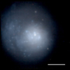 |
Fig. 1. Color image of Haro 14 from the MUSE data (logarithmic intensity scale). A scale bar of 1 kpc (15.9 arcsec) in length is shown to the bottom right. North is at the top and east to the left, as is the case for all the maps presented hereafter. |
Basic data for Haro 14.
In this second paper, we study the ionized gas emission in Haro 14. The wide FoV of MUSE and its unprecedented sensitivity allow observations of a large set of diagnostic emission lines, including the faint [O I]λ6300, out to large galactocentric distances (up to 2.7 kpc) and very low surface brightness levels (about 10−18 erg s−1 cm−2 arcsec−2). This dataset enables us to perform, for the first time, an exhaustive investigation of the nebular morphology and the ionization structure in the very faint outskirts of a BCG.
The paper is structured as follows: in Sect. 2 we briefly summarize the observations and main steps in the data process and introduce the method employed to derive the emission line maps. In Sect. 3 we present the main outcomes from our data analysis, which include a thorough discussion of the Haro 14 spatial pattern in emission lines and in diagnostic line ratios, spatially resolved diagnostic diagrams, and integrated spectroscopy of the galaxy and the most interesting galaxy regions. Finally, the main findings of the work are discussed in Sect. 4 and are summarized in Sect. 5.
2. Observations and data processing
Data on Haro 14 were collected with MUSE (Bacon et al. 2010) at the Very Large Telescope (VLT; ESO Paranal Observatory, Chile). MUSE, working in wide field mode, provides a FoV of 1′×1′ with a spatial sampling of 0 2. We observed in the wavelength range 4750–9300 Å, with a spectral sampling of 1.25 Å pix−1 in the dispersion direction, and an average resolving power of R ∼ 3000. The data were acquired in September 2017 during the science verification of the MUSE Adaptive Optics Facility (AOF; Leibundgut et al. 2017). There is a gap between ∼5800 and 5950 Å, because the AOF works with four sodium lasers and otherwise the detector would saturate in that range.
We took four exposures of Haro 14, each of 1370 s, with a pattern of 90° rotations between exposures, giving a total of 5480 s on source. Because the target fills the MUSE FoV, we took separate sky fields of 120 s between the science exposures. The data were processed using the standard MUSE pipeline (Weilbacher et al. 2016, 2020) working within the ESOREX environment with the default set of calibrations. The complete description of the data reduction and sky subtraction is provided in Paper I.
2.1. Emission line fitting
The next step in the IFS data process is the measurement of the parameters of the emission lines (fluxes, radial velocities, and full width at half maximum, FWHM) required to build the maps. To derive accurate fluxes of emission lines in star forming galaxies is not straightforward, because in every element of spatial resolution the observed spectrum is the sum of the light generated in the nebula and the light emitted by the stars. Particularly problematic is the measurement of the fluxes of the hydrogen Balmer series in emission, because the strength of these lines can be severely affected by the absorption of the underlying population of stars (McCall et al. 1985; Olofsson 1995; González Delgado & Leitherer 1999; Levesque & Leitherer 2013). Single stellar population (SSP) models predict equivalent width values of between 2 and 16 Å during the first 1 Gyr of a solar metallicity burst, with the equivalent widths reaching their maximum at about a few hundred million years, when the stellar population is dominated by A-type stars (González Delgado et al. 1999, 2005).
The influence of the underlying stellar absorption in the integrated spectrum of Haro 14 is already clear from Fig. 2. Sharp absorption wings are visible around Hβ in emission, and more moderate wings are also visible around Hα. An inspection of the spectra of the individual spatial pixels (spaxels) shows that the strengths of the absorption strongly depends on the position across the galaxy (Fig. 3). Therefore, the determination of accurate Balmer fluxes in emission requires modelling the spectral energy distribution (SED) of the stellar component for every spaxel.
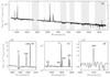 |
Fig. 2. Flux-calibrated integrated spectrum of the BCG Haro 14. (a) Spectrum in the whole observed wavelength range (4750–9300 Å). Shaded bars mark spectral windows heavily contaminated by telluric lines which were excluded from the fitting of the stellar component. The 5800–5950 Å gap corresponds to the spectral area masked out due to the AO lasers. Bottom panels: spectral regions of particular interest, with prominent lines labeled. (b) Zoom into the 4750–5100 Å wavelength region, with the pronounced absorption wings around Hβ clearly resolved. (c) Zoom into the 6250–6800 Å spectral region. (d) Zoom into the region of 9050-9150 Å. |
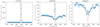 |
Fig. 3. Example fits to the observed spectrum (asterisks) in the vicinity of the Hβ line at three positions in the map (spaxel coordinates on top), illustrating where the emission line is dominant (left panel), severely affected by underlying stellar absorption (central panel), and subdominant (right panel). Red line: stellar component. Black line: stellar plus emission (Gaussian) component. |
Before performing the spectral fit of the stellar component, we grouped the 104006 spectra of the MUSE data cube into bins of similar signal-to-noise ratio (S/N) using the Voronoi adaptive binning algorithm (Cappellari & Copin 2003). We required a S/N on the stellar continuum ≥50 per wavelength channel in each bin in the spectral range 5400–5600 Å and discarded spaxels with S/N ≤ 5. This resulted in a total of 1793 spectra after the binning process.
Next we modeled the SED of these 1793 individual spectra with the Galaxy IFU Spectroscopy Tool (GIST1; Bittner et al. 2019). In a first step, we determined the line-of-sight velocity distribution by means of the penalized pixel-fitting technique (ppxf; Cappellari & Emsellem 2004; Cappellari 2017). This method allows the user to simultaneously fit the optimal linear combination of stellar templates to the observed spectrum and to derive the stellar kinematics, using a maximum likelihood approach to suppress noise solutions. The code convolves the stellar templates with Gauss-Hermite functions to reproduce the shape of the galaxy absorption lines; we considered here only the first four Gauss-Hermite moments (velocity, sigma, h3 and h4). The ppxf technique can work with empirical libraries or with theoretical spectra generated by population synthesis models. We opt for the latter, and use synthesis model templates because they enable more flexibility concerning the spectral range and spectral resolution. We used the Binary Population and Spectral Synthesis models (BPASS, v.2.22; Eldridge & Stanway 2009; Eldridge et al. 2017; Stanway & Eldridge 2018), a relatively new set of population synthesis models that include the effects of binary evolution, conferring a major advantage. The models predict the properties of SSPs at ages from 1 Myr to 100 Gyr in 51 steps (we incorporated 43 steps in our calculations, from 1 to 16 Gyr) and 14 metallicities, from 5 × 10⁻⁵ to 2 Z⊙. We adopted an initial mass function (IMF) with a maximum stellar mass of 100 M⊙ and a broken power law with a slope of −2.0 above 0.5 M⊙ and −1.3 below.
Once the kinematical parameters are known, GIST provides a guess of the spectrum of the underlying stellar population in each bin. After removing this stellar spectrum from the observed one, the emission line parameters are computed making use of the Gas and Absorption Line Fitting software (GandALF; Sarzi et al. 2006; Falcón-Barroso et al. 2006). The emission line spectrum is then removed from the observed one and the ppxf algorithm is run again to obtain the final stellar spectrum of the bin. Spectral regions heavily affected by telluric lines were excluded from the fitting (see Fig. 2).
Finally, the emission-line parameters are calculated on every spaxel by fitting Gaussians plus the estimated stellar spectrum of the corresponding bin. The fit was carried out with the Trust-region algorithm for nonlinear least squares, using the function fit of MATLAB. We run an automatic procedure, which fits a series of lines for every spaxel, namely, Hβ, [O III] λλ4959, 5007, [O I] λλ6300, 6363, Hα, [N II] λλ6548, 6583, [S II] λλ6716, 6731, [Ar III] λ7135, and [S III] λ9069. The fit algorithm provides the relevant parameters of the emission lines (line flux, centroid position, line width) as well as their associated errors.
2.2. Generating the galaxy maps
The parameters derived from the fit (line fluxes, centroid position, line width, and continuum) were then used to build the bidimensional maps of the galaxy. The full wavelength range of MUSE covers a good number of diagnostic emission lines: recombination lines of hydrogen and helium3, high and low ionization, collisionally excited forbidden lines of oxygen and sulfur, and low ionization collisional forbidden lines of nitrogen (see Table 2, and Fig. 2). We built emission line maps of the brighter lines, that is, Hβ, [O III], [O I], Hα, [N II], [S II], [Ar III], and [S III].
Emission lines of Haro 14 in the MUSE observed range for which line maps have been generated.
Line ratio maps were generated by simply dividing the corresponding flux maps. Because the seeing depends on the spectral region observed, when two lines are widely separated (as is the case of the Hα/Hβ and [O III]/Hα maps; see Sects. 3.2 and 3.4) we have corrected for the different seeing. The Hα map was degraded by convolving it with a bi-dimensional Gaussian (σ = 1.2 pix) to match both point spread functions (PSFs). When computing line ratio maps, we included only those spaxels containing values higher than the 3σ level. The maps have not been corrected for interstellar extinction (see Sect. 3.2).
3. Results
3.1. Morphology of the warm ionized gas
The intensity maps of Haro 14 in the brightest emission lines are shown in Figs. 4–6. Maps in Hα and [O III] λ5007 were already presented and briefly discussed in Cairós et al. (2021). The galaxy shows a clumpy morphology, with the brightest knots located in the central regions forming a bar-like arrangement and a horseshoe-like curvilinear feature. These clumps are embedded in an extended halo of ionized gas, from which curvilinear structures such as loops, shells, and filaments emerge. Despite the globally similar appearance, some important differences are evident among the maps in different emission lines, in particular in the dimmer regions of the galaxy periphery.
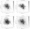 |
Fig. 4. Emission-line flux maps of Haro 14. Top-left: Hβ map, with the central bar-like and curvilinear structures indicated with white lines. Top-right: [O III] λ5007 map. Bottom-left: [O I] λ6300 map; the black lines indicate lobes of enhanced emission in the galaxy periphery. Bottom-right: Hα map. The maps are in logarithmic scale and flux units are 10−20 erg s−1 cm−2 arcsec−2. The red cross indicates the position of the continuum peak and the red line (bottom left) corresponds to 1 kpc. |
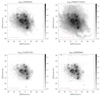 |
Fig. 5. Emission-line flux maps of Haro 14. Top left: [N II] λ6584. Top right: [S II] λλ6717, 6731. Bottom left: [Ar III] λ7135. Bottom right: [S III] λ9068. The maps are in logarithmic scale and flux units are 10−20 erg s−1 cm−2 arcsec−2. The red cross indicates the position of the continuum peak and the red line (bottom left) corresponds to 1 kpc. |
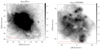 |
Fig. 6. Intensity maps of Haro 14 in Hα (left) and [O I] (right). In the Hα map, the central regions are saturated in order to enhance the faint surface brightness features in the galaxy outskirts; the white lines indicate the most prominent shells and filaments in the galaxy periphery. In the [O I] map, we have zoomed into the HSB area in order to better distinguish its structure; major bubbles and filaments are indicated with white lines. Both maps are in logarithmic scale and flux units are 10−20 erg s−1 cm−2 arcsec−2. |
The maps in Hα and Hβ display the same pattern, but in Hα, which is significantly brighter, the intricate distribution of shells, filaments, holes, and bubbles appears much more clearly. Particularly noteworthy are two curvilinear filaments extending up to 2 and 2.3 kpc southwest, and a shell with a diameter of about 800 pc visible to the north (Fig. 4, bottom-right and Fig. 6, left).
The morphology in the high-ionization [O III] line is roughly similar to Hα in the central area but notable differences appear in the galaxy outskirts. As a general rule, the knots situated in the peripheral zone appear more compact and round in [O III] than in Hα and, although the bulk of the knots are detected in both maps, some of the faintest ones are visible only in Hα or only in [O III]. Remarkably, the large filaments of ionized gas extending southwest and the shell at the north, which are highly visible in Hα, are not detected in [O III] (cf. upper and lower right panels in Fig. 4). The maps in the other two high-ionization lines, namely [Ar III] λ7135 and [S III] λ9069, show the same morphology as [O III] but a poorer S/N, and mostly delineate the HSB central region of the galaxy.
The map in the low-ionization [O I] λ6300 line presents some distinctive features. We see fewer and smaller blobs than in the other line maps. In the central galaxy regions, we discern several bubbles and filaments which are barely detected (if at all) in Hα (Fig. 4, bottom and Fig. 6, right). In the galaxy periphery, the emission is considerably enhanced: we see extended [O I] emission spatially coincident with the southern filaments and northern bubble detected in Hα, but also two large lobes of diffuse emission departing southeast and west, and extending about 1.3 and 1 kpc, respectively (Fig. 4, lower left).
The maps in the low-ionization lines [N II] λ6584 and [S II] λλ6717, 6731 are almost indistinguishable in the central clumpy area, but the brighter sulfur lines delineate the galaxy outskirts much more clearly; both lines reproduce the morphology in Hα very well (Fig. 5, top panels).
The strength and spatial distribution of the different emission lines provide an initial view of the physical processes taking place in a galaxy. While H II-regions are characterized by strong high-ionization emission lines (such as [O III]) and weak low-ionization forbidden lines (such as [N II], [S II], or [O I]), spectra generated by an active galactic nucleus (AGN) or shock heating show a much wider range of ionization, with enhanced emission from both high- and low-ionization forbidden lines (Aller 1984; Veilleux & Osterbrock 1987; Dopita & Sutherland 2003; Osterbrock & Ferland 2006).
In Haro 14, the morphology of the central HSB regions is consistent with SF photoionization: the emission is mainly concentrated in large and bright clumps, which appear very well delineated in recombination (Hα, Hβ) and high-ionization ([O III], [Ar III], [S III]) lines, but are not as clearly defined in the maps of forbidden lines with a low ionization potential ([O I], [N II], [S II]). However, the mechanism responsible for the gas ionization in the galaxy periphery is difficult to establish. The diffuse emission in the Hα and [S II] maps fills almost the whole FoV, extending up to galactocentric distances of ∼2.7 kpc– different scenarios have been proposed to explain how could Lyman continuum photons leaking from H II-regions travel such large distances without being absorbed, but this is still unclear (e.g., Miller & Cox 1993; Dove & Shull 1994; Dove et al. 2000; Hoopes & Walterbos 2003; Giammanco et al. 2005). In addition, kiloparsec-scale (possibly expanding) structures, such as bubbles and filaments, are highly visible in our [O I], Hα, and [S II] maps. The existence of such well-traced structures, which is particularly difficult to reconcile with a scenario of ionization by hot stars, is often interpreted in terms of shocks (Rand 1998; Collins & Rand 2001). This is further explored below by means of diagnostic line ratio maps and diagnostic diagrams.
3.2. Interstellar extinction
The interstellar extinction in a nebula can be computed by comparing the observed Balmer decrement values to the theoretical ones. The Balmer line ratios are known from atomic theory; assuming that deviations from the predicted values are due to absorption by dust, the interstellar extinction coefficient, C(Hβ), is such that
![$$ \begin{aligned} \frac{F_{\lambda }}{F(\mathrm{H}_{\beta })}=\left[\frac{F_{\lambda }}{F(\mathrm{H}_{\beta })}\right]_0\times 10^{-C(\mathrm{H}_{\beta })[f(\lambda )-f(\mathrm{H}_{\beta })]} , \end{aligned} $$](/articles/aa/full_html/2022/08/aa43028-22/aa43028-22-eq9.gif)
where Fλ/F(Hβ) is the observed ratio of Balmer emission-line intensities relative to Hβ, [Fλ/F(Hβ)]0 is the theoretical ratio, and f(λ) is the adopted extinction law (Dopita & Sutherland 2003; Osterbrock & Ferland 2006). Equation (1) can be applied to every spaxel on the frame to determine the spatial distribution of the dust when we work with integral field spectroscopy data.
We generated the interstellar extinction map of Haro 14 from the Hα and Hβ intensity maps. Hα and Hβ have a different PSF, and we have degraded the best-seeing map, convolving with a Gaussian to match both PSFs. We adopted a theoretical ratio of 2.87 (case B recombination at a temperature of 104 K; Osterbrock & Ferland 2006) and used the Galactic extinction law from O’Donnell (1994).
The derived extinction map exhibits a clear spatial pattern (see Fig. 7, top-left). The lowest values of the extinction are found in the areas of intense SF, where F(Hα)/F(Hβ)∼3 (this line ratio implies4 magnitudes of extinction in V of AV = 0.12 and a color excess of E(B − V) = 0.04). The extinction increases considerably when moving toward the periphery of the knots, reaching values of up to F(Hα)/F(Hβ)∼6 (hence, AV = 2 and E(B − V) = 0.64). These results agree very well with our previous VIMOS findings (Cairós & González-Pérez 2017a). The dust accumulates mostly in two zones –located at the southeast and northwest– that are somewhat symmetric with respect to the galaxy center. Such spatial distribution of the dust, with mostly dust-free SF areas and accumulation of dust in the periphery, is consistent with a scenario in which dust is destroyed or swept away by the most massive stars.
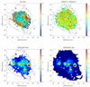 |
Fig. 7. Emission line ratio maps of Haro 14. Top left: balmer decrement, Hα/Hβ. Top right: ratio of the collisional excited sulfur lines, [S II] λλ6717, 6731. Bottom left: excitation map, [O III] λ5007/Hβ. Bottom right: excitation map, [O III] λ5007/Hα. The contour levels of the Hα flux map are overplotted. |
The extinction map is spatially limited by the extent of the Hβ emission, which is considerably fainter than Hα, [O III], or [S II]. This is clearly seen in the top-left panel of Fig. 7, in which we have overplotted the Hα contour maps (but see also Figs. 4 and 5). For this reason, we have not corrected the maps presented in this paper for interstellar reddening: the extinction map presented here gives us an idea of the relative importance of the correction and its spatial variability; a detailed correction at the spaxel level would be of little value.
Large values of interstellar extinction considerably affect the fluxes, magnitudes, and luminosities, but the commonly used diagnostic line ratios ([O III]/Hβ, [S II]/Hα, [N II]/Hα, and [O I]/Hα) are almost insensitive to reddening (for an extinction in V as large as AV = 2, these ratios would change by less than 10%).
3.3. Electron density distribution
Figure 7 (top right) shows a map of the ratio of the collisionally excited sulfur lines, [S II] λλ6717, 6731, which is a sensitive indicator of density in the range 102–104 cm−3 (Aller 1984; Osterbrock & Ferland 2006).
In the central galaxy regions, where the SF is taking place, we find relatively high and homogeneous values of the [S II] λ6717/[S II] λ6731 ratio (≥1.35), indicative of low electron densities (Ne ≤ 100 cm−3). The ratio decreases slightly towards the outer regions, with values of between 1.2 and 0.9 (corresponding to densities 240 cm−3 and 940 cm−3, respectively, at Te = 104 K). Such a density pattern, that is, low density in the areas of SF with increasing density towards the galaxy outskirts, is characteristic of a disturbed ISM, in which the higher densities are associated with filaments that form in the expanding fronts produced by stellar winds and SN explosions (McCray & Kafatos 1987; Tenorio-Tagle & Bodenheimer 1988).
3.4. Diagnostic line ratio maps
A nebula can be excited and ionized by means of different mechanisms, the most common ones being photoionization by OB stars, photoionization by a power-law continuum (AGN), and shock-wave heating (Aller 1984; Dopita & Sutherland 2003; Osterbrock & Ferland 2006). Because the characteristics of the emitted spectrum strongly depend on the power source, the strength and spatial distribution of emission lines can be used to constrain the excitation and ionizing mechanism(s). In particular, emission line intensity ratios involving strong lines, such as [O III]/Hβ, [N II]/Hα, [S II]/Hα, and also [O I]/Hα, are highly sensitive to the properties of the excitation source (Baldwin et al. 1981; Veilleux & Osterbrock 1987). The deep MUSE observations enable us to build line ratio maps that easily reach the galaxy periphery and allow us to probe the ionization structure of Haro 14 up to kiloparsec scales.
Emission line ratio maps of Haro 14, generated as described in Sect. 2.2, are displayed in Figs. 7 and 8. The correction for interstellar extinction is negligible for the classical diagnostic line ratios ([O III]/Hβ, [N II]/Hα, [S II]/Hα, and [O I]/Hα) as the lines of each pair are very close in wavelength, but it does play a role in the [O III]/Hα map (see below).
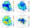 |
Fig. 8. Diagnostic line ratio maps of Haro 14 involving low-ionization lines. Top left: [O I] λ6300/Hα. Top right: [N II] λ6584/Hα. Bottom left: [S II] λλ6717, 6731/Hα. Bottom right: [S II] λλ6717, 6731/[N II] λ6584. The contour levels of the Hα flux map are overplotted. |
The [O III]/Hβ map (bottom left panel in Fig. 7) exhibits an unusual and quite intriguing pattern, with the excitation fluctuating strongly across the galaxy, and showing values ranging from about 0.8 to 5.5. The inner area in the map reproduces our VIMOS findings (Cairós & González-Pérez 2017a): the excitation in the central knots that define the linear and horseshoe-like structures is typical of regions photoionized by hot stars ([O III]/Hβ∼3–3.5), but similarly high values are also found in several areas not associated with bright SF regions. The MUSE excitation map reaches much larger galactocentric distances and clearly demonstrates that [O III]/Hβ does not peak in the central, brightest H II-regions but in several clumps located in the galaxy periphery. The excitation reaches its maximum ([O III]/Hβ ∼ 5.5) in a large blob located ∼12 arcsec (=750 pc) west from the continuum peak (knot Ex1 in Fig. 9). Another high-excitation blob ([O III]/Hβ ∼ 4.5) is situated ∼19 arcsec (1200 pc) east from the center (knot Ex3 in Fig. 9). An interesting excitation peak, elongated and forming an arc, is found in the central bar-like structure (knot Ex8 in Fig. 9). Various other secondary excitation peaks are distinguishable in the southeast region, close to the borders of the mapped area.
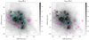 |
Fig. 9. Individual regions of Haro 14 for which an integrated spectrum has been generated, which is overplotted on a Hα flux map. The color of the knots indicates their position in the [O III]/Hβ versus [O I]/Hα diagnostic diagram: knots below the maximum starburst line are shown in blue, and knots above and to the right of the line are shown in magenta (see also Fig. 12). Left panel: emission sources identified in the Hα flux map. Labels correspond to their number (L1, L2, ..., L33) in the catalog of Tables 3, A.1, and A.2. Right panel: regions of high excitation identified in the galaxy. Labels correspond to their number (Ex1, Ex2, ..., Ex16) in the catalog of Tables 4 and 5. |
The spatial extent of [O III]/Hβ is considerably limited because of the relatively weak emission in Hβ. To better visualize the structure of the excitation in the galaxy outskirts, we also built the [O III]/Hα map (Fig. 7, bottom right). The [O III]/Hα ratio is not as commonly used as a diagnostic because it is affected by interstellar extinction, [O III] and Hα being rather far apart in wavelength. Because the effect of extinction would be to lower the [O III] emission with respect to Hα, [O III]/Hα must be understood as a lower bound to the excitation. In the case of Haro 14, the structure of [O III]/Hα closely follows [O III]/Hβ in the areas where they overlap; as the ratio [O III]/Hβ is extinction independent, dust does not seem to affect the spatial structure of the map in these regions.
The [O III]/Hα map traces areas of high excitation in the galaxy outskirts with high fidelity. In this map, we clearly resolve a new blob situated about 24″(1.5 kpc) west from the peak in continuum (knot Ex2 in Fig. 9); interestingly, it aligns with the other very high-excitation blobs in a direction roughly perpendicular to the central SF bar. Several other excitation maxima are detected, most of them lying along two chains in the southeast and the southwest galaxy regions; they delimit a border beyond which the excitation remains uniformly low. As expected, the high-excitation regions correspond to clumps that are brighter and much more clearly traced in the high-ionization [O III] line than in Hα. Most of these high-excitation sources appear compact and roundish in [O III], which suggests that they are associated with SF regions rather than with extended shocked areas. There is one clear exception: the elongated excitation peak (knot Ex8 in Fig. 9).
The [O I]/Hα map (Fig. 8, top-left) displays a similar spatial pattern to the excitation, but here the clumps and/or peaks are not as well delineated. Very low [O I]/Hα (≤0.05) values, characteristic of H II-regions, appear in a band crossing the galaxy east to west in the northern region (0″ ≤ Δ Dec ≤ +18″) and in the whole southwest area. The zone of low [O I]/Hα at the southwest coincides with the interior of the cavity delineated by the large filaments. The galaxy outskirts present mostly high [O I]/Hα, with values of between 0.2 and 0.5–the largest ratios are reached in the areas of enhanced emission in the [O I] intensity map (see Fig. 5, bottom-left).
The [N II]/Hα and [S II]/Hα maps (Fig. 8, top-right and bottom-left) display a similar morphology (also roughly similar to [O I]/Hα), but the outer galaxy regions are better traced in the more extended [S II]/Hα map. In both diagnostic maps, the central clumps appear well delineated and show values characteristic of H II photoionization ([N II]/Hα ≤ 0.15 and [S II]/Hα ≤ 0.5) and the line ratios increase when we move outwards. The ratio [S II]/Hα rises up to 1 in the regions of the periphery that also shows enhanced values of [O I]/Hα.
Photoionization models alone cannot accurately predict [O I]/Hα ≥ 0.2 and [S II]/Hα ≥ 0.8 (see e.g., Mathis 1986; Domgorgen & Mathis 1994; Hoopes & Walterbos 2003); larger values of these diagnostic line ratios have previously been explained in terms of shock heating (Shull & McKee 1979; Dopita & Sutherland 1995; Allen et al. 1999; Rich et al. 2010, 2011).
3.5. Spatially resolved diagnostic diagrams
Line ratio diagnostic diagrams are simple but effective tools to discriminate emission-line galaxies according to their dominant excitation and ionization mechanism (Baldwin et al. 1981; Veilleux & Osterbrock 1987; Kewley et al. 2001a). This technique was originally developed for single-aperture spectroscopy and mostly applied to integrated and nuclear spectra of galaxies (Kewley et al. 2001b, 2006; Kauffmann et al. 2003; Yuan et al. 2010). However, it has gained a new, more profound diagnostic potential with the advent of integral field spectroscopy, in particular in combination with the ability of mapping: tracing individual regions on the diagnostic diagram back to places on the object. Applying the diagnostic diagram approach to integral field data allows the excitation mechanism to be constrained over large galaxy areas and the various power sources operating on the same object to be effectively located and identified (Sharp & Bland-Hawthorn 2010; Rich et al. 2010, 2011, 2014, 2015; Leslie et al. 2014; Davies et al. 2014, 2017; Cairós & González-Pérez 2017a,b, 2020).
Figure 10 presents the [O III]/Hβ versus [O I]/Hα (hereafter, [O I] diagram), [O III]/Hβ versus [N II]/Hα (hereafter, [N II] diagram), and [O III]/Hβ versus [S II]/Hα (hereafter, [S II] diagram) diagnostic diagrams of Haro 14. We represent the line ratios for individual spaxels in the plots, in each case taking into account only those with S/N > 3 in the corresponding lines. In each diagram, we also show the “maximum starburst line” derived by Kewley et al. (2001a), which marks the theoretical limit for gas photoionized by young massive stars: the excitation of spaxels situated above and to the right of this line cannot be explained via SF alone and must have a significant contribution from alternative mechanisms (e.g., shocks or AGNs). The points in the figures are color-coded according to their distance to this maximum starburst line. We note that we have not made use of any rebinning strategy to increase the S/N (one point corresponds to one spaxel); therefore, the density of points in a given region of the diagram faithfully represents the area of the galaxy with those properties.
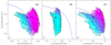 |
Fig. 10. Optical emission line diagnostic diagrams for the individual spaxels in Haro 14. The solid blue line in the panels delineates the theoretical “maximum starburst line” derived by Kewley et al. (2001a); to better visualize the results, the points are color-coded according to their distance to this line. In the three diagrams, the lower-left section of the plot is occupied by spaxels in which the dominant energy source is the radiation from hot stars (blue points in the figure); additional ionizing mechanisms shift the spaxels to the top right and right part of the diagrams (from cyan to pink). The contours show the density of spaxels; each contour level corresponds to a density four times higher than the next outer one. The cross in each diagram gives an estimate of the typical uncertainties on the ratios. The black triangles indicate the diagnostic ratios for the integrated spectrum of the whole galaxy. |
The first result that emerges from Fig. 10 is the large discrepancy between the [N II] (panel b in the figure) and the [O I] and [S II] diagrams (panels a and c). While the [O I] and [S II] diagrams exhibit a similar shape, with the individual spaxels widely spread in both axes, the points appear concentrated in a vertical strip in the [N II] plot; the same behavior was found by Cairós & González-Pérez (2017a), building the diagrams for the smaller FoV of VIMOS. This is expected, because the [N II] diagram is degenerated at low metallicities (0.2 Z⊙ < Z < 0.4 Z⊙), where the areas ionized by shocks and hot stars overlap (Allen et al. 2008; Hong et al. 2013). At the metallicity of Haro 14 (Z ∼ Z⊙/3; Cairós & González-Pérez 2017a), this diagram has a diminished diagnostic power. Therefore, in the following we focus on the findings from the other two plots.
A striking feature of the diagnostic diagrams is the large fraction of spaxels that falls outside the zone corresponding to photoionization by hot stars. The spaxels above the starburst line in the [O I] and [S II] diagrams represent ∼75% and ∼50% of the area of Haro 14, respectively. This is an important result that is in remarkable contrasts with the findings of previous works: in the spatially diagnostic diagrams built for BCGs so far, the majority of datapoints appear situated below the maximum starburst line, from which it has often been concluded that hot massive stars are the dominant power source in these galaxies (Calzetti et al. 2004; James et al. 2010, 2016; Kehrig et al. 2008, 2016; Cresci et al. 2017; Kumari et al. 2017, 2019; Oparin et al. 2020).
The reason for the discrepancy between our findings and those of earlier studies is fundamentally of an observational nature. The dataset analyzed here represents a major advancement with respect to previous works, because of the wider FoV and higher sensitivity provided by MUSE. Regarding IFS-based investigations, the main drawback until now has been their limited FoV, barely covering the starburst regions (e.g., Kehrig et al. 2008; James et al. 2010; Kumari et al. 2017, 2019); but even working with a larger FoV, typical 2–4m telescopes do not allow accurate measurements of the outer regions of BCGs to be obtained within reasonable observing times (e.g., Kehrig et al. 2016). Alternatively, the ionized gas in a sample of nearby starbursts, including several BCGs, was investigated by Calzetti et al. (2004) and Hong et al. (2013) by means of narrow-band imaging from the Hubble Space Telescope (HST). Although the mapped FoV was also restricted mostly to the starburst due to the proximity of the objects, the higher angular resolution of the HST allowed to identify shock-excited regions around the bright star forming clusters. These works reported a small though discernible contribution of shocks. Our VIMOS observations, which included the whole starburst and a significant fraction of the extended emission in Haro 14, Tololo 1937-423, and Mrk 900 also found a significant fraction of spaxels ionized by shocks (Cairós & González-Pérez 2017a,b, 2020).
Therefore, the spatially resolved diagnostic diagrams previously built for BCGs did not allow the power sources operating in the galaxies to be probed, because they simply did not contain information on the whole system. It is not surprising to find that the dominant ionizing mechanism is OB stars, when the observations trace primarily the HSB regions of the galaxy, but this finding should not be extrapolated to the whole galaxy: conclusions regarding the ionizing mechanism acting in the faint galaxy regions should be considered only tentatively. The observations presented here, reaching a surface brightness of about 10−18 erg s−1 cm−2 arcsec−2 in all diagnostic lines (including the faint [O I]λ6300), allowed us, for the first time, to accurately investigate the excitation mechanism operating in the outer regions of a typical BCG.
We display in Fig. 11 the spatial location on the galaxy of the spaxels following the same color code that we employed in the diagnostic diagrams. Here, it is clearly shown that spaxels within the photoionized zone in the diagrams can be traced back to the central SF regions, while the spaxels laying beyond the maximum starburst line correspond mostly to fainter regions in the galaxy outskirts. The spaxels located outside the H II-region ionization zone in the [O I] and [S II] diagrams account for ∼20% and ∼13% of the Hα luminosity, respectively. This is a significant fraction, particularly if we take into account the fact that the maximum starburst line represents a rather conservative approach and that spaxels lying below this line can also have a non-negligible contribution from a harder ionizing source (Kauffmann et al. 2003; Kewley et al. 2006). For comparison, for NGC 4214, NGC 3077, and NGC 5253, Calzetti et al. (2004) reported a fraction of Hα emission contributed by mechanisms other than OB-star photoionization of around 3%–4%.
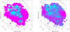 |
Fig. 11. Spaxels represented in the diagnostic diagrams of Haro 14 localized on the galaxy, following the color code in Fig. 10. Contours in Hα are overplotted. Left: spaxels in the [O I] diagram: the largest fraction of the area is being ionized by a mechanism different from SF. Right: spaxels in the [S II] diagram. |
3.6. Integrated spectroscopy
The maps of Haro 14 enable us to identify interesting structures in the galaxy, such as areas of enhanced emission in a particular line, dust patches, and high-excitation blobs. As the next step in our analysis, we produced the integrated spectrum for Haro 14 and for the most distinctive structures, which include the brightest Hα emitters and the regions of highest excitation.
3.6.1. The integrated spectrum of Haro 14
The integrated spectrum of Haro 14 is shown in Fig. 2, and was generated by summing over all spaxels in the observed field. This is the spectrum of a composite stellar population – with bright emission lines (e.g., Hα, Hβ, [O III], [N II], [S II]) characteristic of H II-regions and starbursts – placed on top of a blue and relatively high stellar continuum with evident absorption features, such as the pronounced wings of Hβ and Hα or the Ca II triplet in the near-infrared.
The reddening-corrected emission line intensities (relative to Hβ) for the integrated spectrum are presented in Table 3. Line intensities were calculated taking into account the contribution of the underlying stellar population as described in Sect. 2.1; the interstellar extinction was derived from the Balmer decrement following the standard approach (Sect. 3.2).
Reddening-corrected line intensity ratios, interstellar extinction, diagnostic line ratios, densities, and oxygen abundances for the emission line sources and integrated spectra of Haro 14.
We obtained a total reddening-corrected flux in Hα of 4.6 ± 0.1 × 10⁻¹³ erg s−1cm−2, which translates into a total Hα luminosity of 9.2 ± 0.2 × 1039 erg s−1. From here we estimated the SFR adopting the expression derived in Hunter et al. (2010):

We note that the Hα flux here is significantly lower than the F(Hα) = 7.3 ± 0.1×10⁻¹³erg s−1 cm−2 value we derived from the VIMOS data in a smaller FoV5 (Cairós & González-Pérez 2017a). This discrepancy likely results from differences in the interstellar extinction correction applied: the magnitude increments derived are AV = 0.292 ± 0.027 (MUSE) and AV = 0.819 ± 0.007 (VIMOS). The observed fluxes (without extinction correction) restricted to the smaller FoV of VIMOS are 3.3 ± 0.1 × 10⁻¹³ erg s−1 cm−2 and 3.5 ± 0.1 × 10⁻¹³ erg s−1 cm−2 from the MUSE and VIMOS datasets, respectively, which are also in reasonable good agreement. This confirms that the differences in the corrected values are due to the distinct extinction coefficients adopted.
Large discrepancies in the interstellar extinction coefficients are a consequence of the large uncertainties associated with the determination of the Hβ and Hα fluxes in emission. Obtaining accurate fluxes for the hydrogen Balmer series in emission is a complicated task, because the strengths of these lines can be severely affected by the absorption of the underlying population of stars (Sect. 2.1). Hence, the values of the emission line fluxes are strongly dependent on the method used to correct for absorption. Here, we take into account the contribution of the underlying stellar component by performing a modeling of the SED, which provides more reliable values.
Table 3 also shows the diagnostic line ratios, electron density (Ne), and oxygen abundance (12+log(O/H)) for the integrated spectrum. Ne was computed from the [S II] λ6717/[S II] λ6731 ratio following Osterbrock & Ferland (2006). We estimated the oxygen abundances by adopting the empirical method introduced by Pilyugin & Grebel (2016), which utilizes the intensities of the strong lines [O III] λλ4957,5007, [N II] λλ6548, 6584, and [S II] λλ6717,6731. The relative accuracy of the abundance derived using this method is 0.1 dex. The oxygen abundance, 12+log(O/H) = 8.20, is in excellent agreement with the value found from the VIMOS data (12+log(O/H) = 8.25).
The position of the line ratios computed from the integrated spectrum is shown in the diagnostic diagrams of Haro 14 (Fig. 10). Interestingly, in the [O I] diagram, the galaxy falls almost exactly on top of the maximum starburst line.
3.6.2. Integrated spectroscopy of Hα emission line sources
The most evident structures in the emission line maps of Haro 14 are the compact clumps visible up to large galactocentric distances; although the largest and brightest ones appear in the central regions of the galaxy. In Paper I, we developed a routine to automatically detect and spatially delimit these sources (for a complete description of the process, see Sect. 3.6.2 in Paper I). By running this routine in the Hα flux map, we identified a total of 40 sources and generated a catalog with their main properties, including position, size, and fluxes in the brightest lines (see Sect. 3.6, Fig. 5, and Table 4 in Paper I).
Here, we performed a more detailed study of these individual clumps. Because we aim to obtain reliable interstellar reddening coefficients and diagnostic line ratios, we restrict ourselves to sources with a S/N greater than 5 in Hβ. In this way, we ended up with the 30 emission line knots that appear identified in Fig. 9 (we note that we keep the number scheme introduced in Paper I, and refer to these knots as L1, L2, etc. throughout the text). Table 3 shows the reddening-corrected emission line fluxes and diagnostic line ratios for the first ten sources, which include the central brightest ones; results for the remaining sources are provided in Appendix A.
Diagnostic diagrams built from the line ratio of these Hα sources are shown in Fig. 12. The majority of the clumps are located below the maximum starburst line, but still a large fraction (10 and 9 knots in the [O I] and [S II] diagrams, respectively) fall outside of the star forming area. The bright sources that constitute the central bar-like and bubble structure are classified, as expected, as H II-region complexes (knots in cyan in Fig. 12). By contrast, most of the Hα sources located in the galaxy periphery lie well above or to the right of the maximum starburst line (shown in magenta in the figure).
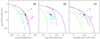 |
Fig. 12. As in Fig. 10, but for the integrated spectra of the individual sources detected in Hα. The black triangles indicate the diagnostic ratios for the integrated spectrum of the whole galaxy. The red and green lines are the photoionization models from Kewley et al. (2001a) for metallicities 0.5 Z⊙ and 0.2 Z⊙. |
The H II regions present a distribution of excitation and ionization similar to the spatially resolved diagnostic diagram. The highest excitation appears in the three brightest SF regions (L1, L2, L3), closest to the center of the galaxy, whereas the lowest excitation is found in three sources (L17, L21, and L22) located between 0.6 and 1 kpc northeast. The distribution of the H II-regions in the diagnostic diagrams – roughly along the maximum starburst line – closely follows the predictions of theoretical photoionization models for different ionization parameters (q) at a fixed metallicity (Dopita et al. 2000; Kewley et al. 2001a). The variation in q would be compatible with a broad range in age for the ionizing stellar clusters.
The Hα sources located above the maximum starburst line form two groups: Three sources (L25, L26 and L28) have very high excitation ([O III]/Hβ ≥ 4); they are indeed the excitation maxima of the galaxy. The remaining sources present excitations of ∼1.5. Five out of the seven low-excitation sources (L20, L24, L27, L29, and L33) form a chain along the southeastern border of the bright ionization region of the galaxy (see Fig. 9). The nature of these sources is difficult to assess. Different mechanisms might be responsible for the ionization of the gas here, and singling out one of them is not obvious.
Table 3 also presents the densities and oxygen abundances of the Hα clumps. All clumps except L33 show densities in the low range, typical of regions of SF; the abundances are homogeneous considering the uncertainties, but there is a tendency to lower abundances in the outer galaxy regions.
3.6.3. Integrated spectroscopy of the high-excitation blobs
The excitation maps of Haro 14 reveal a large number of maxima distributed irregularly across the galaxy; interestingly, the zones of highest excitation do not spatially coincide with the brightest SF complexes, but are situated in the periphery of the HSB galaxy regions (Sect. 3.4). The large number of high-excitation clumps and, in particular, the fact that the peaks are located outside of the SF area are puzzling. The global properties of these regions, derived from their integrated spectra, will help to shed some light on the physical processes acting there.
We detected and spatially delimited these high-excitation regions using the same procedure as for the Hα sources (Sect. 3.6.3 and Paper I). In this case, we ran the routine in the [O III]/Hα map and detected 16 clumps. Tables 4 and 5 present the reddening-corrected intensity ratios, the interstellar extinction coefficient, the diagnostic line ratios and the oxygen abundances for each knot.
Reddening-corrected line intensity ratios, interstellar extinction, diagnostic line ratios, densities, and oxygen abundances for the high-excitation blobs in Haro 14.
Reddening-corrected line intensity ratios, interstellar extinction, diagnostic line ratios, densities, and oxygen abundances for the high excitation blobs in Haro 14.
Figure 13 displays the diagnostic diagrams for the high-excitation blobs. Only five are situated within the hot star photoionization area of the diagram (in both [O I] and [S II]), while most of them fall outside the starburst line. The knots under the starburst line roughly coincide with knots 1, 2, 3, 5, and 8 in Hα: they are bright H II-regions whose high excitation reflects the high temperature of the ionizing stars. However, the nature of the knots above the starburst line is difficult to determine. They span a wide range of excitation, and although two groups are somehow suggested, they are not clearly defined. Their position in the diagram is consistent with different types of interstellar shocks, but their morphology, in many cases, suggests regions of SF. Particularly interesting are the three knots aligned to the north, which constitute the galaxy excitation peaks.
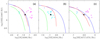 |
Fig. 13. As in Fig. 10, but for the integrated spectra of the high-excitation blobs. The solid blue line in the panels delineates the theoretical “maximum starburst line” derived by Kewley et al. (2001a). The black triangles indicate the diagnostic ratios for the integrated spectrum of the whole galaxy. The red and green lines are the photoionization models from Kewley et al. (2001a) for metallicities 0.5 Z⊙ and 0.2 Z⊙. |
4. Discussion
MUSE allowed us to observe not only the central HSB star forming regions of Haro 14, but also the ionized halo and faint structures that dominate the emission at large galactocentric distances, and with unprecedented depth. This is an exceptional asset with respect to previous BCGs works, as it is in these dimmer regions of the galaxy periphery that we expect to see the feedback mechanisms at work and where alternative ionization sources (e.g., shock heating, evolved stellar populations, or the dilute radiation from photoionizing sources) are expected to play a major role.
4.1. The diverse ionizing mechanisms operating in Haro 14
Considering both the morphology and the surface brightness, the emission line maps of Haro 14 present two different components: a HSB region made of individual clumps, which occupies the central galaxy zones, and a LSB component, which extends up to kiloparsec scales and consists of widespread diffuse emission, clearly delineated curvilinear structures, and faint clumps6.
The HSB area exhibits the same clumpy morphology in all lines, which is also apparent in the diagnostic maps, where the clumps are clearly delineated and spatially coincide with maxima in the excitation and minima in the other ratios. This is characteristic of areas photoionized by massive hot stars.
By contrast, the LSB component shows marked differences among the emission in different lines. For example, several clumps and filaments are visible in some lines but not in others. All diagnostic maps present variability on large spatial scales in the galaxy periphery. Most of the LSB area displays low values of [O III]/Hβ and high values of [O I]/Hα, [N II]/Hα, and [S II]/Hα, an ionization pattern usually interpreted in terms of diluted radiation from OB stars or shock-heating (Mathis 1986, 2000; Dopita & Sutherland 2003; Haffner et al. 2009). However, [O I]/Hα and [S II]/Hα are extremely high in various zones (up to 0.5 and 1, respectively); these large values cannot be explained in terms of OB stars alone, as photoionization models do not predict ratios significantly larger than [O I]/Hα ∼ 0.2 and [S II]/Hα ∼ 0.8 (e.g., Domgorgen & Mathis 1994; Hoopes & Walterbos 2003). In starburst systems, such enhanced [O I]/Hα and [S II]/Hα in the galaxy periphery have previously been associated with shock excitation (Calzetti et al. 2004; Veilleux & Rupke 2002; Monreal-Ibero et al. 2006, 2010; Sharp & Bland-Hawthorn 2010; Rich et al. 2010, 2011). Interestingly, in the galaxy outskirts, we also find regions of very high excitation and low values of the other ratios; indeed, the excitation peaks are located there, in two knots placed ∼750 and 1600 pc to the west of the continuum peak, and a third one located ∼1200 pc to the east. The ionization source operating here is not evident; we come back to this point in Sect. 4.1.2.
We make these arguments quantitative by building the spatially resolved diagnostic line ratio diagrams of Haro 14 (Fig. 10). According to their position in these diagrams, most spaxels in the galaxy are being ionized by a mechanism other than SF: adopting the maximum starburst line proposed in Kewley et al. (2001b) we find that in ∼75% and ∼50% of the galaxy area (in the [O I] and [S II] diagrams, respectively) an alternative mechanism is operating. This corroborates the finding of the galaxy maps, which show that the central clumpy area is made of photoionized H II regions whereas an additional mechanism of ionization (and most probably, more than one) is required to explain the values of the line ratios all over the LSB area (Fig. 11).
In contrast to the spaxels falling below the starburst line, it is not straightforward to associate an excitation mechanism(s) to those above the line. The traditional approach distinguishes two sectors here: the AGN and the low-ionization narrow emission line region (LINER) domains (Kewley et al. 2001a, 2006; Kauffmann et al. 2003). However, it is now well established that other mechanisms can generate line ratios mimicking those of AGNs and LINERs, such as interstellar shocks (Sharp & Bland-Hawthorn 2010; Farage et al. 2010; Rich et al. 2010, 2011, 2015), energetic photons leaking out from H II-regions (Hidalgo-Gámez 2005, 2007; Weilbacher et al. 2018; Belfiore et al. 2022), or hot low-mass evolved stars (HOLMES; Flores-Fajardo et al. 2011; Zhang et al. 2017; Belfiore et al. 2016, 2022).
From the diagnostic diagrams alone we cannot discriminate between these different sources, but interpreting their results together with the morphology and ionization structure revealed by the maps will allow us to put additional constraints on the physical process(es) responsible for the ionization in the galaxy outskirts.
4.1.1. Below the maximum starburst line
The spaxels that fall below the maximum starburst line in the diagnostic diagrams correspond spatially with the clumps that comprise the central bar-like and the horseshoe-shaped features (Figs. 4 and 11), confirming that the central clumps are large complexes of H II-regions.
This H II-region photoionized area in the diagram spans a broad range in excitation (∼1.2 dex) and follows a sequence that runs almost parallel to the maximum starburst line. The distribution of the points along this sequence can be interpreted as variations in the ionization parameter which, in turn, may be reflecting the large range of ages of the ionizing clusters, as is expected in an extended (kiloparsec scales) starburst such as the one observed in Haro 14. This is consistent with the [O III]/Hα line ratio maps, in which there is an evident excitation gradient among the central clumps, and is also further corroborated by the diagnostic diagram of the individual Hα sources (Fig. 9), in which the SF knots define the same excitation sequence as that seen in the spaxel resolved diagrams.
Stellar clusters with different ages naturally arise in different scenarios of SF; for example, sequential SF resulting from the impact of massive stellar evolution in the surrounding ISM (Elmegreen & Lada 1977; Whitworth et al. 1994) or continuous SF, as in a merger or interaction event. In the case of Haro 14, the observations are consistent with both scenarios: massive clusters, whose evolution must have produced a large number of SN events, are present in the galaxy, but also the morphology is suggestive of past interactions or mergers (Cairós et al. 2021); we note that neither scenario excludes the other. The presence of a marked age gradient among the H II-regions in Haro 14 is an interesting phenomenon, and will be addressed in more detail in a forthcoming publication where we will use synthesis population models to reproduce the observables of the individual clusters.
Similar spaxel distributions below the maximum starburst line have been found for NGC 4214 (Calzetti et al. 2004), Mrk 900 (Cairós & González-Pérez 2020), and Tololo 1937-423 (Cairós & González-Pérez 2017b), objects that also present an extended area of ongoing SF made of multiple H II-region complexes. In Haro 14 (as well as in NGC 4214), the galaxy inclination (we see the galaxy almost face on) allows us to resolve individual sources that in edge-on galaxies would appear integrated along the line of sight.
4.1.2. Beyond the maximum starburst line
As we state above, it is not straightforward to identify the mechanism responsible for the ionization of the spaxels above the maximum starburst line. In the case of Haro 14, an AGN can be naturally discarded, but to discriminate between shocks and other mechanisms on the basis of line ratios alone is rather difficult.
Some information can be extracted from the distribution of the points in the diagnostic diagrams. The individual spaxels span a huge range in excitation, with [O III]/Hβ up to 10; however, the individual Hα and high-excitation sources do not extend over the whole excitation range, but appear split into two groups, with the Hα sources being much more clearly defined (Figs. 12 and 13). The large variation in excitation together with the fact that the individual sources appear gathered in groups point to more than one power source acting in the galaxy outskirts. Also, that the spaxels cover a broad and densely populated area (Fig. 10) means that the ionization conditions vary in a continuous manner; as expected, for instance, when the ionizing photons are diluted radiation.
Additional information can be derived from the morphology and ionization pattern associated with these spaxels. The spaxels beyond the maximum starburst line encompass the whole LSB component (Fig. 11); that is, they include the diffuse extended halo, coherent and likely expanding structures (such as filaments and shells), and several faint clumps (see Figs. 4, 5, and 11). It seems a plausible hypothesis that these different morphologies arise from different physical processes; it would be indeed difficult to identify a unique mechanism able to originate the three of them.
The morphology of the diffuse constituent is consistent with the ionization being produced by the dilute radiation from OB stars. In this scenario, the ionization structure changes gradually as we move away from the central heating source. Because the most energetic photons are absorbed close to the exciting stars, the hardness of the radiation (and the excitation) decreases with the distance while the line ratios of the low-ionization species increases (Miller & Cox 1993; Dove & Shull 1994; Domgorgen & Mathis 1994; Haffner et al. 2009). This produces a smooth distribution of ionized gas that can extend to large distances, in which the excitation anti-correlates with the Hα surface brightness (Ferguson et al. 1996; Zurita et al. 2000, 2002). This is the behaviour that we observe in the largest fraction of the LSB ionized gas in Haro 14 (see the bottom panels of Fig. 7).
The most striking features in the LSB regions of Haro 14 are the numerous curvilinear features (filaments, loops, and shells) departing from the central HSB areas and extending up to kiloparsec scales. The morphology suggests shock excitation, with the ionized filaments and shells being the edges of giant expanding bubbles associated with supernova-driven galactic winds (Marlowe et al. 1995; Lehnert & Heckman 1996; Martin 1998; Strickland et al. 2004a,b; Book et al. 2008; Egorov et al. 2014, 2017, 2018). Particularly eye-catching are the two filaments extending up to 2 and 2.3 kpc southwest (Fig. 6). Similar filaments have been observed in other BCGs and local starbursts (e.g., NGC 1569, Heckman et al. 1995; Martin 1998; Buckalew & Kobulnicky 2006; Westmoquette et al. 2008; NGC 3077, Martin 1998; Ott et al. 2003; Oparin et al. 2020; and Henize 2-10, Méndez et al. 1999; Johnson et al. 2000; Cresci et al. 2017), and were interpreted as signatures of bipolar flows connected with nuclear starburst activity.
Finally, the mechanism responsible for the ionization of the LSB clumps in the galaxy periphery is more difficult to determine unequivocally. The fact that these sources split into two groups in the diagnostic diagrams (Figs. 12 and 13) points to different kinds of objects; otherwise we would expect a smooth transition. The morphological pattern of the knots with lower ionization suggests they were generated in shocked areas, as most of them are distributed in a chain depicting the border between the high- and low-surface-brightness gas components (Fig. 9, left panel); in this scenario the clumps may be the debris of fragmented shells and/or filaments. The nature of the high ionization knots is puzzling; in particular, the three clumps that coincide with peaks in the excitation maps (1, 2, and 3 in Fig. 9 and Table 4). These three knots, which fall in the AGN zone of the diagnostic diagram mostly due to their high excitation, appear aligned in a direction roughly orthogonal to the central SF bar. Their morphology suggests large SF complexes, but their diagnostic ratios imply different physical conditions from those found in typical H II-regions; they are also very different from the SF regions in the central areas. Several mechanisms can contribute to alter the values of the excitation in H II-regions; for example, the presence of dust, variations in the metallicity, or the fact that these are density-limited regions. In Haro 14, neither the dust contribution nor the oxygen abundances seem to play a significant role: the ionized clumps with high excitation present interstellar extinction values and oxygen abundances in the same range as those of the central H II-regions (see Table A.2).
A more complete study that includes the analysis of the kinematical results is required to further investigate and disentangle the nature of the distinct power sources acting in the galaxy periphery. This will be addressed in a forthcoming publication.
4.2. Some remarks on the spatially resolved diagnostic diagrams of Haro 14
Spatially resolved diagnostic diagrams are fundamentally different tools from the classic diagrams introduced to classify galaxies based on their integrated spectra. Rather than from a single point in a graph, a galaxy is now characterized by a distribution of points giving the relationship between the diagnostic line ratios throughout the observed area. This allows us to identify and probe different power sources acting in the same object and, in combination with the spectral maps, to determine their spatial position. In addition, the characteristics of the cloud of points (e.g., its extent, shape, or density) may provide additional information that helps to reconstruct a consistent picture of the physical processes taking place in the galaxy and their impact on the surrounding ISM.
Some features on the spatially resolved diagnostic diagrams of Haro 14 (Fig. 10) merit further discussion. In particular, because these diagrams show notable quantitative and qualitative differences with respect to the BCG diagnostic diagrams presented in previous works (e.g., Calzetti et al. 2004; Kehrig et al. 2008, 2016, 2018; Kehrig et al. 2020; James et al. 2010, 2016; Lagos et al. 2012, 2014; Hong et al. 2013; Cresci et al. 2017; Cairós & González-Pérez 2017a,b, 2020). We focused here on the [O I] and [S II] diagrams of Haro 14, because the [N II] diagram loses its diagnostic power at low metallicities (see Sect. 3.5).
The most salient features of the diagrams of Haro 14 are the following:
-
They appear quite crowded, with the data points densely covering a well-defined and quite extended area spanning more than 1.5 dex in excitation and [O I]/Hα, and 1 dex in [S II]/Hα. This is a consequence of the larger FoV, the higher spatial resolution, and the higher sensitivity of the observations.
-
The data points in the [O I] and the [S II] diagrams spread symmetrically over a broad strip of up to 1.5 dex in width, and roughly along the maximum starburst line.
-
There is a well-defined, curved exclusion zone at large excitation ([O III]/Hβ ≥ 3) that segregates the points into two symmetrical populations, one either side of the maximum starburst line.
-
At low excitation ([O III]/Hβ ≤ 0.3), there is a gradual concentration around the maximum starburst line ([O I]/Hα ∼ 0.1 and [S II]/Hα ∼ 0.6).
These features confer to the diagnostic diagrams the distinctive shape of a butterfly, a general arrangement that could already be seen, though much less clearly, in the diagrams of Haro 14 built from VIMOS data (Cairós & González-Pérez 2017a). Interestingly, this characteristic shape is also visible in the diagrams of the BCGs Mrk 900 (Cairós & González-Pérez 2020) and Tololo 1937-423 (Cairós & González-Pérez 2017b). It would be interesting to explore whether or not this butterfly shape also appears in the diagnostic diagrams of other BCGs and, if so, how often and for which conditions. Such an analysis, which requires observations reaching similar surface brightness levels in the galaxy outskirts for a number of objects, is out of the scope of this paper. We address this question in a forthcoming publication of this series, currently under preparation.
5. Conclusions
This is the second paper in a series reporting the results of a MUSE/VLT based study of the BCG Haro 14. Here, we performed an exhaustive analysis of the properties of the warm ionized gas emission in the galaxy. Capitalizing on the large FoV (3.8 × 3.8 kpc2 at the adopted distance) of MUSE and its unprecedented sensitivity, we investigated the morphology, dust distribution, physical properties, and ionization structure of the ionized gas, not only in the central HSB galaxy regions but also in the LSB areas of the periphery; this is an important achievement with respect to previous integral field spectroscopy of BCGs.
An additional advantage of our deep observational strategy is that MUSE made possible to obtain reliable measurements of the faint [O I]λ6300 line up to kiloparsec scales. Maps of this line at large galactocentric distances are essential if we aim to explore the contribution of shocks to the global ionization (Dopita 1976; Dopita & Sutherland 1996), as is the case here. However, the detection of [O I]λ6300 in galaxies has so far been quite challenging: this line is not only extremely faint, but in the Milky-Way and nearby objects it becomes strongly contaminated by the bright (∼100 times brighter than the interstellar line) [O I]λ6300 airglow line (Reynolds et al. 1998; Voges & Walterbos 2006).
From our analysis of the extremely rich MUSE dataset, we highlight the following results:
-
The ongoing SF episode in Haro 14 extends up to kiloparsec scales, with the brightest H II-region complexes located close to the galaxy center. These H II-regions show large variations in the excitation, which likely reflect a range of ages in the ionizing clusters.
-
An extended and faint halo of ionized gas encircles the H II-regions complexes. This halo is not smooth, but here we resolved well-defined curvilinear structures, such as arcs, shells, filaments, and compact clumps. Particularly noteworthy are the two curvilinear filaments extending up to 2 and 2.3 kpc southwest, and a shell with a diameter about 800 pc to the north.
-
We find evidence of a photoionization mechanism other than young massive stars operating in Haro 14. The central HSB component is mostly made of H II-region complexes, but an additional heating source is required to explain the line ratios and morphological pattern in the whole LSB component. Indeed, the largest fraction of the galaxy area is being ionized by one (or several) alternative power source(s): spaxels above the maximum starburst line represent ∼75% and ∼50% of the area in the [O I] and [S II] diagrams respectively and account for ∼20% and ∼13% of the Hα luminosity, respectively. This result contrasts with previous BCG investigations, with the reason for this discrepancy lying fundamentally in the observations: our data, reaching surface brightnesses of about 10−18 erg s−1 cm−2 arcsec−2 in all diagnostic lines (including the faint [O I]λ6300), allowed us, for the first time, to come to robust conclusions as to the excitation mechanism operating in the outer regions of a typical BCG.
-
Both the morphology and the distribution of the spaxels in the diagnostic diagrams point to different mechanisms acting in the galaxy periphery. The three distinct morphological constituents of the LSB ionized gas, that is, the widespread diffuse halo, the filamentary structures, and the individual clumps, are likely ionized by different mechanisms. We suggest that the extended halo is being ionized by diluted radiation escaping from the central H II-regions, and that the large filaments and shells are shocked areas in the walls of expanding bubbles associated with outflows. The mechanism responsible for the ionization of the individual clumps is more difficult to asses. The power sources acting in the galaxy outskirts will be investigated in a forthcoming publication based on kinematical results.
In conclusion, this work stresses the important role played by wide-field integral field instruments such as MUSE in BCG research and, in particular, in the study of their warm ionized gas. At the typical distances of BCGs (between 10 and 40 Mpc), MUSE allows us to map the whole system, making it possible to characterize the ionized gas at large galactocentric distances. Constraining the ionizing source, not just in the central galaxy regions but also in the galaxy outskirts, enables us to separate areas of the galaxy ionized by hot stars from areas where other mechanisms are responsible for the ionization. This makes it possible to derive accurate ages, abundances, and excitation patterns, leading to a much better characterization of the SF event. However, investigations of the outskirts of BCGs are not only important in the context of dwarf galaxy research and nearby starbursts, but are also essential in cosmological studies, as it is in the galaxy outskirts where primordial gas may still be accreting today.
GIST is a modular pipeline, entirely written in Python 3, developed for the scientific analysis of reduced integral field spectroscopic data: http://ascl.net/1907.025.
With AV = 2.1 × C(Hβ) and E(B − V) = 0.697 × C(Hβ), following Dopita & Sutherland (2003).
The gas outside classical H II-regions appears commonly referred to in the literature as diffuse ionized gas (DIG) or warm ionized medium (WIM). These terms comprise the three different constituents that we mention here: the smooth extended emission, the filamentary structures, and the faint blobs.
Acknowledgments
LMC acknowledges support from the Deutsche Forschungsgemeinschaft (CA 1243/1-1 and CA 1234/1-2). PMW received support from BMBF Verbundforschung (project VLT-BlueMUSE, grant 05A20BAB). Based on observations collected at the European Southern Observatory under ESO programme ID 60.A-9186(A). This research has made use of the NASA/IPAC Extragalactic Database (NED), which is operated by the Jet Propulsion Laboratory, Caltech, under contract with the National Aeronautics and Space Administration. We acknowledge the usage of the HyperLeda database (http://leda.univ-lyon1.fr). This work made use of v2.2.1 of the Binary Population and Spectral Synthesis (BPASS) models as described in Eldridge et al. (2017) and Stanway & Eldridge (2018). We used IRAF package, which are distributed by the National Optical Astronomy Observatory, which is operated by the Association of Universities for Research in Astronomy, Inc., under contract with the National Science Foundation.
References
- Allen, M. G., Dopita, M. A., Tsvetanov, Z. I., & Sutherland, R. S. 1999, ApJ, 511, 686 [NASA ADS] [CrossRef] [Google Scholar]
- Allen, M. G., Groves, B. A., Dopita, M. A., Sutherland, R. S., & Kewley, L. J. 2008, ApJS, 178, 20 [Google Scholar]
- Aller, L. H. 1984, Astrophys. Space Sci. Lib. (D. Reidel Publishing Company), 12 [CrossRef] [Google Scholar]
- Bacon, R., Accardo, M., Adjali, L., et al. 2010. Proc. SPIE, 7735, 773508 [Google Scholar]
- Baldwin, J. A., Phillips, M. M., & Terlevich, R. 1981, PASP, 93, 5 [Google Scholar]
- Bekki, K. 2008, MNRAS, 388, L10 [Google Scholar]
- Belfiore, F., Maiolino, R., Maraston, C., et al. 2016, MNRAS, 461, 3111 [Google Scholar]
- Belfiore, F., Santoro, F., Groves, B., et al. 2022, A&A, 659, A26 [NASA ADS] [CrossRef] [EDP Sciences] [Google Scholar]
- Bik, A., Östlin, G., Hayes, M., et al. 2015, A&A, 576, L13 [NASA ADS] [CrossRef] [EDP Sciences] [Google Scholar]
- Bik, A., Östlin, G., Menacho, V., et al. 2018, A&A, 619, A131 [NASA ADS] [CrossRef] [EDP Sciences] [Google Scholar]
- Bittner, A., Falcón-Barroso, J., Nedelchev, B., et al. 2019, A&A, 628, A117 [NASA ADS] [CrossRef] [EDP Sciences] [Google Scholar]
- Book, L. G., Chu, Y.-H., & Gruendl, R. A. 2008, ApJS, 175, 165 [NASA ADS] [CrossRef] [Google Scholar]
- Brosch, N., Almoznino, E., & Heller, A. B. 2004, MNRAS, 349, 357 [NASA ADS] [CrossRef] [Google Scholar]
- Buckalew, B. A., & Kobulnicky, H. A. 2006, AJ, 132, 1061 [NASA ADS] [CrossRef] [Google Scholar]
- Cairós, L. M., & González-Pérez, J. N. 2017a, A&A, 600, A125 [NASA ADS] [CrossRef] [EDP Sciences] [Google Scholar]
- Cairós, L. M., & González-Pérez, J. N. 2017b, A&A, 608, A119 [NASA ADS] [CrossRef] [EDP Sciences] [Google Scholar]
- Cairós, L. M., & González-Pérez, J. N. 2020, A&A, 634, A95 [NASA ADS] [CrossRef] [EDP Sciences] [Google Scholar]
- Cairós, L. M., Vílchez, J. M., González Pérez, J. N., Iglesias-Páramo, J., & Caon, N. 2001, ApJS, 133, 321 [CrossRef] [Google Scholar]
- Cairós, L. M., Caon, N., Zurita, C., et al. 2009a, A&A, 507, 1291 [NASA ADS] [CrossRef] [EDP Sciences] [Google Scholar]
- Cairós, L. M., Caon, N., Papaderos, P., et al. 2009b, ApJ, 707, 1676 [CrossRef] [Google Scholar]
- Cairós, L. M., González-Pérez, J. N., Weilbacher, P. M., & Manso Sainz, R. 2021, A&A, 654, A142 [NASA ADS] [CrossRef] [EDP Sciences] [Google Scholar]
- Calzetti, D., Harris, J., Gallagher, I., J. S., et al. 2004, AJ, 127, 1405 [NASA ADS] [CrossRef] [Google Scholar]
- Cappellari, M. 2017, MNRAS, 466, 798 [Google Scholar]
- Cappellari, M., & Copin, Y. 2003, MNRAS, 342, 345 [Google Scholar]
- Cappellari, M., & Emsellem, E. 2004, PASP, 116, 138 [Google Scholar]
- Collins, J. A., & Rand, R. J. 2001, ApJ, 551, 57 [NASA ADS] [CrossRef] [Google Scholar]
- Cresci, G., Vanzi, L., Telles, E., et al. 2017, A&A, 604, A101 [NASA ADS] [CrossRef] [EDP Sciences] [Google Scholar]
- Davies, R. L., Rich, J. A., Kewley, L. J., & Dopita, M. A. 2014, MNRAS, 439, 3835 [Google Scholar]
- Davies, R. L., Groves, B., Kewley, L. J., et al. 2017, MNRAS, 470, 4974 [NASA ADS] [CrossRef] [Google Scholar]
- Dekel, A., & Silk, J. 1986, ApJ, 303, 39 [Google Scholar]
- de Vaucouleurs, G., de Vaucouleurs, A., Corwin, H. G., Jr, et al. 1991, Third Reference Catalogue of Bright Galaxies, Sky and Telescope, 82, 621 [Google Scholar]
- De Young, D. S., & Heckman, T. M. 1994, ApJ, 431, 598 [NASA ADS] [CrossRef] [Google Scholar]
- Domgorgen, H., & Mathis, J. S. 1994, ApJ, 428, 647 [NASA ADS] [CrossRef] [Google Scholar]
- Dopita, M. A. 1976, ApJ, 209, 395 [NASA ADS] [CrossRef] [Google Scholar]
- Dopita, M. A., & Sutherland, R. S. 1995, ApJ, 455, 468 [Google Scholar]
- Dopita, M. A., & Sutherland, R. S. 1996, ApJS, 102, 161 [Google Scholar]
- Dopita, M. A., & Sutherland, R. S. 2003, Astrophysics of the Diffuse Universe [CrossRef] [Google Scholar]
- Dopita, M. A., Kewley, L. J., Heisler, C. A., & Sutherland, R. S. 2000, ApJ, 542, 224 [NASA ADS] [CrossRef] [Google Scholar]
- Dove, J. B., & Shull, J. M. 1994, ApJ, 430, 222 [NASA ADS] [CrossRef] [Google Scholar]
- Dove, J. B., Shull, J. M., & Ferrara, A. 2000, ApJ, 531, 846 [NASA ADS] [CrossRef] [Google Scholar]
- Egorov, O. V., Lozinskaya, T. A., Moiseev, A. V., & Smirnov-Pinchukov, G. V. 2014, MNRAS, 444, 376 [NASA ADS] [CrossRef] [Google Scholar]
- Egorov, O. V., Lozinskaya, T. A., Moiseev, A. V., & Shchekinov, Y. A. 2017, MNRAS, 464, 1833 [NASA ADS] [CrossRef] [Google Scholar]
- Egorov, O. V., Lozinskaya, T. A., Moiseev, A. V., & Smirnov-Pinchukov, G. V. 2018, MNRAS, 478, 3386 [NASA ADS] [CrossRef] [Google Scholar]
- Eldridge, J. J., & Stanway, E. R. 2009, MNRAS, 400, 1019 [NASA ADS] [CrossRef] [Google Scholar]
- Eldridge, J. J., Stanway, E. R., Xiao, L., et al. 2017, PASA, 34 [Google Scholar]
- Elmegreen, B. G., & Lada, C. J. 1977, ApJ, 214, 725 [Google Scholar]
- Elmegreen, B. G., Zhang, H.-X., & Hunter, D. A. 2012, ApJ, 747, 105 [NASA ADS] [CrossRef] [Google Scholar]
- Falcón-Barroso, J., Bacon, R., Bureau, M., et al. 2006, MNRAS, 369, 529 [Google Scholar]
- Farage, C. L., McGregor, P. J., Dopita, M. A., & Bicknell, G. V. 2010, ApJ, 724, 267 [NASA ADS] [CrossRef] [Google Scholar]
- Federrath, C. 2015, MNRAS, 450, 4035 [Google Scholar]
- Ferguson, A. M. N., Wyse, R. F. G., Gallagher, I., J. S., & Hunter, D. A. 1996, AJ, 111, 2265 [NASA ADS] [CrossRef] [Google Scholar]
- Flores-Fajardo, N., Morisset, C., Stasińska, G., & Binette, L. 2011, MNRAS, 415, 2182 [Google Scholar]
- García-Lorenzo, B., Cairós, L. M., Caon, N., Monreal-Ibero, A., & Kehrig, C. 2008, ApJ, 677, 201 [CrossRef] [Google Scholar]
- Gerola, H., Seiden, P. E., & Schulman, L. S. 1980, ApJ, 242, 517 [NASA ADS] [CrossRef] [Google Scholar]
- Giammanco, C., Beckman, J. E., & Cedrés, B. 2005, A&A, 438, 599 [NASA ADS] [CrossRef] [EDP Sciences] [Google Scholar]
- Gil de Paz, A., Madore, B. F., & Pevunova, O. 2003, ApJS, 147, 29 [NASA ADS] [CrossRef] [Google Scholar]
- González Delgado, R. M., & Leitherer, C. 1999, ApJS, 125, 479 [CrossRef] [Google Scholar]
- González Delgado, R. M., Leitherer, C., & Heckman, T. M. 1999, ApJS, 125, 489 [CrossRef] [Google Scholar]
- González Delgado, R. M., Cerviño, M., Martins, L. P., Leitherer, C., & Hauschildt, P. H. 2005, MNRAS, 357, 945 [Google Scholar]
- Haffner, L. M., Dettmar, R. J., Beckman, J. E., et al. 2009, Rev. Mod. Phys., 81, 969 [CrossRef] [Google Scholar]
- Heckman, T. M., Armus, L., & Miley, G. K. 1990, ApJS, 74, 833 [Google Scholar]
- Heckman, T. M., Dahlem, M., Lehnert, M. D., et al. 1995, ApJ, 448, 98 [NASA ADS] [CrossRef] [Google Scholar]
- Herenz, E. C., Hayes, M., Papaderos, P., et al. 2017, A&A, 606, L11 [NASA ADS] [CrossRef] [EDP Sciences] [Google Scholar]
- Hidalgo-Gámez, A. M. 2005, A&A, 442, 443 [NASA ADS] [CrossRef] [EDP Sciences] [Google Scholar]
- Hidalgo-Gámez, A. M. 2007, AJ, 134, 1447 [CrossRef] [Google Scholar]
- Hong, S., Calzetti, D., Gallagher, J. S., III, et al. 2013, ApJ, 777, 63 [NASA ADS] [CrossRef] [Google Scholar]
- Hoopes, C. G., & Walterbos, R. A. M. 2003, ApJ, 586, 902 [NASA ADS] [CrossRef] [Google Scholar]
- Hunter, D. 1997, PASP, 109, 937 [NASA ADS] [CrossRef] [Google Scholar]
- Hunter, D. A., & Elmegreen, B. G. 2004, AJ, 128, 2170 [NASA ADS] [CrossRef] [Google Scholar]
- Hunter, D. A., & Elmegreen, B. G. 2006, ApJS, 162, 49 [NASA ADS] [CrossRef] [Google Scholar]
- Hunter, D. A., & Gallagher, I., J. S. 1986, PASP, 98, 5 [NASA ADS] [CrossRef] [Google Scholar]
- Hunter, D. A., Elmegreen, B. G., & Ludka, B. C. 2010, AJ, 139, 447 [NASA ADS] [CrossRef] [Google Scholar]
- James, B. L., Tsamis, Y. G., & Barlow, M. J. 2010, MNRAS, 401, 759 [NASA ADS] [CrossRef] [Google Scholar]
- James, B. L., Tsamis, Y. G., Walsh, J. R., Barlow, M. J., & Westmoquette, M. S. 2013a, MNRAS, 430, 2097 [NASA ADS] [CrossRef] [Google Scholar]
- James, B. L., Tsamis, Y. G., Barlow, M. J., Walsh, J. R., & Westmoquette, M. S. 2013b, MNRAS, 428, 86 [NASA ADS] [CrossRef] [Google Scholar]
- James, B. L., Auger, M., Aloisi, A., Calzetti, D., & Kewley, L. 2016, ApJ, 816, 40 [Google Scholar]
- Johnson, K. E., Leitherer, C., Vacca, W. D., & Conti, P. S. 2000, AJ, 120, 1273 [NASA ADS] [CrossRef] [Google Scholar]
- Kauffmann, G., Heckman, T. M., Tremonti, C., et al. 2003, MNRAS, 346, 1055 [Google Scholar]
- Kehrig, C., Vílchez, J. M., Sánchez, S. F., et al. 2008, A&A, 477, 813 [NASA ADS] [CrossRef] [EDP Sciences] [Google Scholar]
- Kehrig, C., Vílchez, J. M., Pérez-Montero, E., et al. 2016, MNRAS, 459, 2992 [NASA ADS] [CrossRef] [Google Scholar]
- Kehrig, C., Vílchez, J. M., Guerrero, M. A., et al. 2018, MNRAS, 480, 1081 [NASA ADS] [Google Scholar]
- Kehrig, C., Iglesias-Páramo, J., Vílchez, J. M., et al. 2020, MNRAS, 498, 1638 [NASA ADS] [CrossRef] [Google Scholar]
- Kewley, L. J., Heisler, C. A., Dopita, M. A., & Lumsden, S. 2001a, ApJS, 132, 37 [Google Scholar]
- Kewley, L. J., Dopita, M. A., Sutherland, R. S., Heisler, C. A., & Trevena, J. 2001b, ApJ, 556, 121 [Google Scholar]
- Kewley, L. J., Groves, B., Kauffmann, G., & Heckman, T. 2006, MNRAS, 372, 961 [Google Scholar]
- Krumholz, M. R., Bate, M. R., Arce, H. G., et al. 2014, in Protostars and Planets VI, eds. H. Beuther, R. S. Klessen, C. P. Dullemond, & T. Henning, 243 [Google Scholar]
- Kumari, N., James, B. L., & Irwin, M. J. 2017, MNRAS, 470, 4618 [NASA ADS] [CrossRef] [Google Scholar]
- Kumari, N., James, B. L., Irwin, M. J., & Aloisi, A. 2019, MNRAS, 485, 1103 [NASA ADS] [CrossRef] [Google Scholar]
- Lagos, P., Telles, E., Nigoche Netro, A., & Carrasco, E. R. 2012, MNRAS, 427, 740 [NASA ADS] [CrossRef] [Google Scholar]
- Lagos, P., Papaderos, P., Gomes, J. M., Smith Castelli, A. V., & Vega, L. R. 2014, A&A, 569, A110 [NASA ADS] [CrossRef] [EDP Sciences] [Google Scholar]
- Larson, R. B. 1974, MNRAS, 169, 229 [NASA ADS] [CrossRef] [Google Scholar]
- Lehnert, M. D., & Heckman, T. M. 1996, ApJ, 462, 651 [NASA ADS] [CrossRef] [Google Scholar]
- Leibundgut, B., Bacon, R., Jaffé, Y. L., et al. 2017, The Messenger, 170, 20 [NASA ADS] [Google Scholar]
- Leslie, S. K., Rich, J. A., Kewley, L. J., & Dopita, M. A. 2014, MNRAS, 444, 1842 [NASA ADS] [CrossRef] [Google Scholar]
- Levesque, E. M., & Leitherer, C. 2013, ApJ, 779, 170 [NASA ADS] [CrossRef] [Google Scholar]
- MacKenty, J. W., Maíz-Apellániz, J., Pickens, C. E., Norman, C. A., & Walborn, N. R. 2000, AJ, 120, 3007 [NASA ADS] [CrossRef] [Google Scholar]
- Mac Low, M.-M., & Ferrara, A. 1999, ApJ, 513, 142 [NASA ADS] [CrossRef] [Google Scholar]
- Marlowe, A. T., Heckman, T. M., Wyse, R. F. G., & Schommer, R. 1995, ApJ, 438, 563 [NASA ADS] [CrossRef] [Google Scholar]
- Marlowe, A. T., Meurer, G. R., Heckman, T. M., & Schommer, R. 1997, ApJS, 112, 285 [NASA ADS] [CrossRef] [Google Scholar]
- Martin, C. L. 1997, ApJ, 491, 561 [NASA ADS] [CrossRef] [Google Scholar]
- Martin, C. L. 1998, ApJ, 506, 222 [NASA ADS] [CrossRef] [Google Scholar]
- Martínez-Delgado, D., Romanowsky, A. J., Gabany, R. J., et al. 2012, ApJ, 748, L24 [CrossRef] [Google Scholar]
- Mathis, J. S. 1986, ApJ, 301, 423 [NASA ADS] [CrossRef] [Google Scholar]
- Mathis, J. S. 2000, ApJ, 544, 347 [NASA ADS] [CrossRef] [Google Scholar]
- McCall, M. L., Rybski, P. M., & Shields, G. A. 1985, ApJS, 57, 1 [CrossRef] [Google Scholar]
- McCray, R., & Kafatos, M. 1987, ApJ, 317, 190 [NASA ADS] [CrossRef] [Google Scholar]
- McKee, C. F., & Ostriker, E. C. 2007, ARA&A, 45, 565 [Google Scholar]
- McQuinn, K. B. W., Skillman, E. D., Heilman, T. N., Mitchell, N. P., & Kelley, T. 2018, MNRAS, 477, 3164 [NASA ADS] [CrossRef] [Google Scholar]
- McQuinn, K. B. W., van Zee, L., & Skillman, E. D. 2019, ApJ, 886, 74 [NASA ADS] [CrossRef] [Google Scholar]
- Menacho, V., Östlin, G., Bik, A., et al. 2019, MNRAS, 487, 3183 [CrossRef] [Google Scholar]
- Menacho, V., Bik, G. Ö. A., Adamo, A., et al. 2021, MNRAS, 506, 1777 [NASA ADS] [CrossRef] [Google Scholar]
- Méndez, D. I., Esteban, C., Filipović, M. D., et al. 1999, A&A, 349, 801 [NASA ADS] [Google Scholar]
- Miller, W. W. I., & Cox, D. P. 1993, ApJ, 417, 579 [NASA ADS] [CrossRef] [Google Scholar]
- Monreal-Ibero, A., Arribas, S., & Colina, L. 2006, ApJ, 637, 138 [Google Scholar]
- Monreal-Ibero, A., Arribas, S., Colina, L., et al. 2010, A&A, 517, A28 [NASA ADS] [CrossRef] [EDP Sciences] [Google Scholar]
- Naab, T., & Ostriker, J. P. 2017, ARA&A, 55, 59 [Google Scholar]
- O’Donnell, J. E. 1994, ApJ, 422, 158 [Google Scholar]
- Oey, M. S., Watson, A. M., Kern, K., & Walth, G. L. 2005, AJ, 129, 393 [NASA ADS] [CrossRef] [Google Scholar]
- Olofsson, K. 1995, A&AS, 111, 57 [NASA ADS] [Google Scholar]
- Oparin, D. V., Egorov, O. V., & Moiseev, A. V. 2020, Astrophys. Bull., 75, 361 [NASA ADS] [CrossRef] [Google Scholar]
- Osterbrock, D. E., & Ferland, G. J. 2006, Astrophysics of Gaseous Nebulae and Active Galactic Nuclei (Sausalito, CA: University Science Books) [Google Scholar]
- Östlin, G., Amram, P., Bergvall, N., et al. 2001, A&A, 374, 800 [NASA ADS] [CrossRef] [EDP Sciences] [Google Scholar]
- Ott, J., Martin, C. L., & Walter, F. 2003, ApJ, 594, 776 [NASA ADS] [CrossRef] [Google Scholar]
- Paudel, S., Duc, P. A., & Ree, C. H. 2015, AJ, 149, 114 [CrossRef] [Google Scholar]
- Paudel, S., Smith, R., Yoon, S. J., Calderón-Castillo, P., & Duc, P.-A. 2018, ApJS, 237, 36 [Google Scholar]
- Pearson, S., Besla, G., Putman, M. E., et al. 2016, MNRAS, 459, 1827 [NASA ADS] [CrossRef] [Google Scholar]
- Pilyugin, L. S., & Grebel, E. K. 2016, MNRAS, 457, 3678 [NASA ADS] [CrossRef] [Google Scholar]
- Privon, G. C., Stierwalt, S., Patton, D. R., et al. 2017, ApJ, 846, 74 [CrossRef] [Google Scholar]
- Pustilnik, S. A., Kniazev, A. Y., Lipovetsky, V. A., & Ugryumov, A. V. 2001, A&A, 373, 24 [NASA ADS] [CrossRef] [EDP Sciences] [Google Scholar]
- Rand, R. J. 1998, ApJ, 501, 137 [NASA ADS] [CrossRef] [Google Scholar]
- Reynolds, R. J., Hausen, N. R., Tufte, S. L., & Haffner, L. M. 1998, ApJ, 494, L99 [NASA ADS] [CrossRef] [Google Scholar]
- Rich, J. A., Dopita, M. A., Kewley, L. J., & Rupke, D. S. N. 2010, ApJ, 721, 505 [NASA ADS] [CrossRef] [Google Scholar]
- Rich, J. A., Kewley, L. J., & Dopita, M. A. 2011, ApJ, 734, 87 [NASA ADS] [CrossRef] [Google Scholar]
- Rich, J. A., Kewley, L. J., & Dopita, M. A. 2014, ApJ, 781, L12 [Google Scholar]
- Rich, J. A., Kewley, L. J., & Dopita, M. A. 2015, ApJS, 221, 28 [Google Scholar]
- Salzer, J. J., & Norton, S. A. 1999, in The Low Surface Brightness Universe, eds. J. I. Davies, C. Impey, & S. Phillipps, ASP Conf. Ser., 170, 253 [NASA ADS] [Google Scholar]
- Sarzi, M., Falcón-Barroso, J., Davies, R. L., et al. 2006, MNRAS, 366, 1151 [Google Scholar]
- Seigar, M. S., & James, P. A. 2002, MNRAS, 337, 1113 [NASA ADS] [CrossRef] [Google Scholar]
- Sharp, R. G., & Bland-Hawthorn, J. 2010, ApJ, 711, 818 [Google Scholar]
- Shi, F., Kong, X., Li, C., & Cheng, F. Z. 2005, A&A, 437, 849 [NASA ADS] [CrossRef] [EDP Sciences] [Google Scholar]
- Shu, F. H., Milione, V., Gebel, W., et al. 1972, ApJ, 173, 557 [NASA ADS] [CrossRef] [Google Scholar]
- Shull, J. M., & McKee, C. F. 1979, ApJ, 227, 131 [Google Scholar]
- Somerville, R. S., & Davé, R. 2015, ARA&A, 53, 51 [Google Scholar]
- Stanway, E. R., & Eldridge, J. J. 2018, MNRAS, 479, 75 [NASA ADS] [CrossRef] [Google Scholar]
- Stierwalt, S., Besla, G., Patton, D., et al. 2015, ApJ, 805, 2 [NASA ADS] [CrossRef] [Google Scholar]
- Strickland, D. K., Heckman, T. M., Colbert, E. J. M., Hoopes, C. G., & Weaver, K. A. 2004a, ApJS, 151, 193 [Google Scholar]
- Strickland, D. K., Heckman, T. M., Colbert, E. J. M., Hoopes, C. G., & Weaver, K. A. 2004b, ApJ, 606, 829 [NASA ADS] [CrossRef] [Google Scholar]
- Tenorio-Tagle, G., & Bodenheimer, P. 1988, ARA&A, 26, 145 [NASA ADS] [CrossRef] [Google Scholar]
- Thuan, T. X. 2008, in Low-Metallicity Star Formation: From the First Stars to Dwarf Galaxies, eds. L. K. Hunt, S. C. Madden, & R. Schneider, IAU Symp., 255, 348 [NASA ADS] [Google Scholar]
- Thuan, T. X., & Martin, G. E. 1981, ApJ, 247, 823 [NASA ADS] [CrossRef] [Google Scholar]
- Thuan, T. X., Lipovetsky, V. A., Martin, J. M., & Pustilnik, S. A. 1999, A&AS, 139, 1 [NASA ADS] [CrossRef] [EDP Sciences] [Google Scholar]
- Vanzi, L., Cresci, G., Telles, E., & Melnick, J. 2008, A&A, 486, 393 [NASA ADS] [CrossRef] [EDP Sciences] [Google Scholar]
- Vanzi, L., Cresci, G., Sauvage, M., & Thompson, R. 2011, A&A, 534, A70 [NASA ADS] [CrossRef] [EDP Sciences] [Google Scholar]
- Veilleux, S., & Osterbrock, D. E. 1987, ApJS, 63, 295 [Google Scholar]
- Veilleux, S., & Rupke, D. S. 2002, ApJ, 565, L63 [NASA ADS] [CrossRef] [Google Scholar]
- Veilleux, S., Cecil, G., & Bland-Hawthorn, J. 2005, ARA&A, 43, 769 [NASA ADS] [CrossRef] [Google Scholar]
- Voges, E. S., & Walterbos, R. A. M. 2006, ApJ, 644, L29 [NASA ADS] [CrossRef] [Google Scholar]
- Walch, S. K., Whitworth, A. P., Bisbas, T., Wünsch, R., & Hubber, D. 2012, MNRAS, 427, 625 [NASA ADS] [CrossRef] [Google Scholar]
- Watts, A., & Bekki, K. 2016, MNRAS, 462, 3314 [NASA ADS] [CrossRef] [Google Scholar]
- Weilbacher, P. M., Streicher, O., & Palsa, R. 2016, Astrophysics Source Code Library [record ascl:1610.004] [Google Scholar]
- Weilbacher, P. M., Monreal-Ibero, A., Verhamme, A., et al. 2018, A&A, 611, A95 [NASA ADS] [CrossRef] [EDP Sciences] [Google Scholar]
- Weilbacher, P. M., Palsa, R., Streicher, O., et al. 2020, A&A, 641, A28 [NASA ADS] [CrossRef] [EDP Sciences] [Google Scholar]
- Westmoquette, M. S., Smith, L. J., & Gallagher, J. S. 2008, MNRAS, 383, 864 [Google Scholar]
- Whitworth, A. P., Bhattal, A. S., Chapman, S. J., Disney, M. J., & Turner, J. A. 1994, A&A, 290, 421 [NASA ADS] [Google Scholar]
- Yuan, T. T., Kewley, L. J., & Sanders, D. B. 2010, ApJ, 709, 884 [NASA ADS] [CrossRef] [Google Scholar]
- Zhang, K., Yan, R., Bundy, K., et al. 2017, MNRAS, 466, 3217 [NASA ADS] [CrossRef] [Google Scholar]
- Zhang, H.-X., Paudel, S., Smith, R., et al. 2020a, ApJ, 891, L23 [CrossRef] [Google Scholar]
- Zhang, H.-X., Smith, R., Oh, S.-H., et al. 2020b, ApJ, 900, 152 [NASA ADS] [CrossRef] [Google Scholar]
- Zurita, A., Rozas, M., & Beckman, J. E. 2000, A&A, 363, 9 [Google Scholar]
- Zurita, A., Beckman, J. E., Rozas, M., & Ryder, S. 2002, A&A, 386, 801 [NASA ADS] [CrossRef] [EDP Sciences] [Google Scholar]
Appendix A: Supplementary tables
Reddening-corrected line intensity ratios, interstellar extinction, diagnostic line ratios, densities, and oxygen abundances for the emission line sources of Haro 14.
Reddening-corrected line intensity ratios, interstellar extinction, diagnostic line ratios, densities, and oxygen abundances for the emission line sources of Haro 14.
All Tables
Emission lines of Haro 14 in the MUSE observed range for which line maps have been generated.
Reddening-corrected line intensity ratios, interstellar extinction, diagnostic line ratios, densities, and oxygen abundances for the emission line sources and integrated spectra of Haro 14.
Reddening-corrected line intensity ratios, interstellar extinction, diagnostic line ratios, densities, and oxygen abundances for the high-excitation blobs in Haro 14.
Reddening-corrected line intensity ratios, interstellar extinction, diagnostic line ratios, densities, and oxygen abundances for the high excitation blobs in Haro 14.
Reddening-corrected line intensity ratios, interstellar extinction, diagnostic line ratios, densities, and oxygen abundances for the emission line sources of Haro 14.
Reddening-corrected line intensity ratios, interstellar extinction, diagnostic line ratios, densities, and oxygen abundances for the emission line sources of Haro 14.
All Figures
|
Fig. 1. Color image of Haro 14 from the MUSE data (logarithmic intensity scale). A scale bar of 1 kpc (15.9 arcsec) in length is shown to the bottom right. North is at the top and east to the left, as is the case for all the maps presented hereafter. |
| In the text | |
|
Fig. 2. Flux-calibrated integrated spectrum of the BCG Haro 14. (a) Spectrum in the whole observed wavelength range (4750–9300 Å). Shaded bars mark spectral windows heavily contaminated by telluric lines which were excluded from the fitting of the stellar component. The 5800–5950 Å gap corresponds to the spectral area masked out due to the AO lasers. Bottom panels: spectral regions of particular interest, with prominent lines labeled. (b) Zoom into the 4750–5100 Å wavelength region, with the pronounced absorption wings around Hβ clearly resolved. (c) Zoom into the 6250–6800 Å spectral region. (d) Zoom into the region of 9050-9150 Å. |
| In the text | |
|
Fig. 3. Example fits to the observed spectrum (asterisks) in the vicinity of the Hβ line at three positions in the map (spaxel coordinates on top), illustrating where the emission line is dominant (left panel), severely affected by underlying stellar absorption (central panel), and subdominant (right panel). Red line: stellar component. Black line: stellar plus emission (Gaussian) component. |
| In the text | |
|
Fig. 4. Emission-line flux maps of Haro 14. Top-left: Hβ map, with the central bar-like and curvilinear structures indicated with white lines. Top-right: [O III] λ5007 map. Bottom-left: [O I] λ6300 map; the black lines indicate lobes of enhanced emission in the galaxy periphery. Bottom-right: Hα map. The maps are in logarithmic scale and flux units are 10−20 erg s−1 cm−2 arcsec−2. The red cross indicates the position of the continuum peak and the red line (bottom left) corresponds to 1 kpc. |
| In the text | |
|
Fig. 5. Emission-line flux maps of Haro 14. Top left: [N II] λ6584. Top right: [S II] λλ6717, 6731. Bottom left: [Ar III] λ7135. Bottom right: [S III] λ9068. The maps are in logarithmic scale and flux units are 10−20 erg s−1 cm−2 arcsec−2. The red cross indicates the position of the continuum peak and the red line (bottom left) corresponds to 1 kpc. |
| In the text | |
|
Fig. 6. Intensity maps of Haro 14 in Hα (left) and [O I] (right). In the Hα map, the central regions are saturated in order to enhance the faint surface brightness features in the galaxy outskirts; the white lines indicate the most prominent shells and filaments in the galaxy periphery. In the [O I] map, we have zoomed into the HSB area in order to better distinguish its structure; major bubbles and filaments are indicated with white lines. Both maps are in logarithmic scale and flux units are 10−20 erg s−1 cm−2 arcsec−2. |
| In the text | |
|
Fig. 7. Emission line ratio maps of Haro 14. Top left: balmer decrement, Hα/Hβ. Top right: ratio of the collisional excited sulfur lines, [S II] λλ6717, 6731. Bottom left: excitation map, [O III] λ5007/Hβ. Bottom right: excitation map, [O III] λ5007/Hα. The contour levels of the Hα flux map are overplotted. |
| In the text | |
|
Fig. 8. Diagnostic line ratio maps of Haro 14 involving low-ionization lines. Top left: [O I] λ6300/Hα. Top right: [N II] λ6584/Hα. Bottom left: [S II] λλ6717, 6731/Hα. Bottom right: [S II] λλ6717, 6731/[N II] λ6584. The contour levels of the Hα flux map are overplotted. |
| In the text | |
|
Fig. 9. Individual regions of Haro 14 for which an integrated spectrum has been generated, which is overplotted on a Hα flux map. The color of the knots indicates their position in the [O III]/Hβ versus [O I]/Hα diagnostic diagram: knots below the maximum starburst line are shown in blue, and knots above and to the right of the line are shown in magenta (see also Fig. 12). Left panel: emission sources identified in the Hα flux map. Labels correspond to their number (L1, L2, ..., L33) in the catalog of Tables 3, A.1, and A.2. Right panel: regions of high excitation identified in the galaxy. Labels correspond to their number (Ex1, Ex2, ..., Ex16) in the catalog of Tables 4 and 5. |
| In the text | |
|
Fig. 10. Optical emission line diagnostic diagrams for the individual spaxels in Haro 14. The solid blue line in the panels delineates the theoretical “maximum starburst line” derived by Kewley et al. (2001a); to better visualize the results, the points are color-coded according to their distance to this line. In the three diagrams, the lower-left section of the plot is occupied by spaxels in which the dominant energy source is the radiation from hot stars (blue points in the figure); additional ionizing mechanisms shift the spaxels to the top right and right part of the diagrams (from cyan to pink). The contours show the density of spaxels; each contour level corresponds to a density four times higher than the next outer one. The cross in each diagram gives an estimate of the typical uncertainties on the ratios. The black triangles indicate the diagnostic ratios for the integrated spectrum of the whole galaxy. |
| In the text | |
|
Fig. 11. Spaxels represented in the diagnostic diagrams of Haro 14 localized on the galaxy, following the color code in Fig. 10. Contours in Hα are overplotted. Left: spaxels in the [O I] diagram: the largest fraction of the area is being ionized by a mechanism different from SF. Right: spaxels in the [S II] diagram. |
| In the text | |
|
Fig. 12. As in Fig. 10, but for the integrated spectra of the individual sources detected in Hα. The black triangles indicate the diagnostic ratios for the integrated spectrum of the whole galaxy. The red and green lines are the photoionization models from Kewley et al. (2001a) for metallicities 0.5 Z⊙ and 0.2 Z⊙. |
| In the text | |
|
Fig. 13. As in Fig. 10, but for the integrated spectra of the high-excitation blobs. The solid blue line in the panels delineates the theoretical “maximum starburst line” derived by Kewley et al. (2001a). The black triangles indicate the diagnostic ratios for the integrated spectrum of the whole galaxy. The red and green lines are the photoionization models from Kewley et al. (2001a) for metallicities 0.5 Z⊙ and 0.2 Z⊙. |
| In the text | |
Current usage metrics show cumulative count of Article Views (full-text article views including HTML views, PDF and ePub downloads, according to the available data) and Abstracts Views on Vision4Press platform.
Data correspond to usage on the plateform after 2015. The current usage metrics is available 48-96 hours after online publication and is updated daily on week days.
Initial download of the metrics may take a while.