| Issue |
A&A
Volume 664, August 2022
|
|
|---|---|---|
| Article Number | A48 | |
| Number of page(s) | 11 | |
| Section | The Sun and the Heliosphere | |
| DOI | https://doi.org/10.1051/0004-6361/202142711 | |
| Published online | 04 August 2022 | |
Coronal loop kink oscillation periods derived from the information of density, magnetic field, and loop geometry
1
School of Astronomy and Space Science and Key Laboratory for Modern Astronomy and Astrophysics, Nanjing University, Nanjing 210023, PR China
e-mail: This email address is being protected from spambots. You need JavaScript enabled to view it.
2
Solar Physics and Space Plasma Research Center (SP2RC), School of Mathematics and Statistics, University of Sheffield, Sheffield S3 7RH, UK
3
Department of Astronomy, Eötvös Lorand University, Pázmány Péter sétány 1/A, Budapest 1117, Hungary
4
Gyula Bay Zoltan Solar Observatory (GSO), Hungarian Solar Physics Foundation (HSPF), Petőfi tér 3., Gyula 5700, Hungary
Received:
21
November
2021
Accepted:
9
May
2022
Abstract
Context. Coronal loop oscillations can be triggered by solar eruptions, for example, and are observed frequently by the Atmospheric Imaging Assembly (AIA) on board Solar Dynamics Observatory (SDO). The Helioseismic and Magnetic Imager (HMI) on board SDO offers us the opportunity to measure the photospheric vector magnetic field and carry out solar magneto-seismology (SMS).
Aims. By applying SMS, we aim to verify the consistency between the observed period and the one derived from the information of coronal density, magnetic field, and loop geometry, that is, the shape of the loop axis.
Methods. We analysed the data of three coronal loop oscillation events detected by SDO/AIA and SDO/HMI. First, we obtained oscillation parameters by fitting the observational data. Second, we used a differential emission measure (DEM) analysis to diagnose the temperature and density distribution along the coronal loop. Subsequently, we applied magnetic field extrapolation to reconstruct the three-dimensional magnetic field and then, finally, used the shooting method to compute the oscillation periods from the governing equation.
Results. The average magnetic field determined by magnetic field extrapolation is consistent with that derived by SMS. A new analytical solution is found under the assumption of exponential density profile and uniform magnetic field. The periods estimated by combining the coronal density and magnetic field distribution and the associated loop geometry are closest to the observed ones, and are more realistic than when the loop geometry is regarded as being semi-circular or having a linear shape.
Conclusions. The period of a coronal loop is sensitive to not only the density and magnetic field distribution but also the loop geometry.
Key words: Sun: corona / Sun: oscillations / Sun: magnetic fields
© G. Y. Chen et al. 2022
 Open Access article, published by EDP Sciences, under the terms of the Creative Commons Attribution License (https://creativecommons.org/licenses/by/4.0), which permits unrestricted use, distribution, and reproduction in any medium, provided the original work is properly cited.
This article is published in open access under the Subscribe-to-Open model. This email address is being protected from spambots. You need JavaScript enabled to view it. to support open access publication.
1. Introduction
Coronal loop oscillations, which are frequently triggered by occasional explosions, such as coronal mass ejections (CMEs) or magnetic flux rope eruptions, can be used to diagnose the physical parameters of the local plasma environment, which are difficult to measure directly (Roberts et al. 1984). In particular, the well-characterised transversal kink oscillation is a typical mode of coronal loop oscillations, which was first detected by Transition Region And Coronal Explorer (TRACE) in 1999 (Aschwanden et al. 1999, 2002; Schrijver et al. 1999, 2002; Nakariakov et al. 1999). Approximating a coronal loop as a magnetic flux tube with uniform magnetic field strength and density distribution, the Alfvén speed can be estimated by measuring the period of the kink oscillations (Roberts et al. 1984; Ruderman & Erdélyi 2009; Aschwanden & Schrijver 2011; Aschwanden et al. 2013). With an empirical ratio of external to internal density, namely ε = ne/ni ∼ 0.1 (Nakariakov et al. 1999; Nakariakov & Ofman 2001), the magnitude of the average magnetic field strength can then be estimated (Roberts et al. 1984).
Early observations revealed the fundamental mode of kink oscillations. The first overtone of coronal loop kink oscillations was detected for the first time by analysing the high temporal and spatial resolution data from TRACE (Verwichte et al. 2004). The ratio between the period of fundamental mode and the first overtone was found to deviate from 2, a canonical value of a straight loop with uniform magnetic field and density distribution, implying non-uniformity of the coronal loops. Since then, with the commissioning of the Solar Dynamics Observatory (SDO, Pesnell et al. 2012), finer coronal loop oscillation events with the first overtone have been observed (Guo et al. 2015; Pascoe et al. 2016; Li et al. 2017; Duckenfield et al. 2018). Moreover, using wavelet analysis, Duckenfield et al. (2019) found a coronal loop oscillation event with a second overtone but without an obvious first overtone. The detection of these high-order overtones has become an effective means to analyse the dynamics of coronal loops and to derive their physical parameters.
From a theoretical perspective, Andries et al. (2005), Goossens et al. (2006), and Van Doorsselaere et al. (2007) worked out the relationship between the period ratio P1/P2 and the density stratification, where P1 and P2 correspond to the periods of the fundamental and the first overtone modes, respectively. Dymova & Ruderman (2005) derived the governing equation for the kink mode oscillation of magnetic flux tube by linearising the magnetohydrodynamics (MHD) equations. Their work provides a valuable basis for investigating the eigenfunction of the kink oscillations. For instance, Erdélyi & Verth (2007) derived three analytic solutions of the governing equations, with assumptions of a step function, a linear function, and a hyperbolic cosine density profile, in conjunction with constant magnetic field, respectively. These authors also obtained a numerical solution to the case with an exponentially stratified density profile. Additionally, Scott & Ruderman (2012) considered the effect of a non-planar loop, and Ruderman et al. (2017) discussed the influence of cross-section expansion. Many of the above aspects were discussed by Andries et al. (2009).
While oscillation-based solar magneto-seismology (SMS) can be applied to estimate the local magnetic field of a coronal loop, one can also use a magnetic field model to obtain the three-dimensional (3D) magnetic field in the corona, including the local magnetic field of a coronal loop. These magnetic field models include potential field, linear force-free field, and non-linear force-free field (NLFFF) models. For example, in the Cartesian coordinate system, a linear force-free field equation can be solved with the Green’s function method and a Fourier transform method (Schmidt 1964; Chiu & Hilton 1977; Seehafer 1978). For a potential field in the spherical coordinate system, the governing equation is reduced to the Laplace equation, ∇2Φ = 0, and B = −∇Φ, where the spherical harmonic transformation technique can be used (Schatten et al. 1969; Newkirk & Altschuler 1969; Schrijver & De Rosa 2003). The results of Guo et al. (2015) showed that the magnetic field of a coronal loop obtained with a potential field model is consistent with that derived with the oscillation-based SMS. In addition, the 3D morphology can be reconstructed from the extrapolated magnetic field, or can alternatively be obtained using stereoscopic observations and the triangulation method.
Coronal loop oscillations are described by a number of coupled physical and geometric parameters. In previous investigations, the density and magnetic field, which dominate the dynamics of a coronal loop, were the research focus. In the present paper, the loop geometry is taken into account, in addition to the density and magnetic field, using a comprehensive approach. Specifically, oscillation periods are obtained from the oscillation evolution time–distance diagram; the density distribution is detected using a DEM analysis; and the geometry and magnetic field are reconstructed by magnetic field extrapolation. The obtained physical and geometric parameters are substituted into the governing equation to determine the computed periods. We show that, in the case of linearised MHD equations, a coronal loop oscillation can be treated as a single string oscillation. Also, we consider three typical configurations for the coronal loop geometry, as follows: (1) Under the assumption of a linear loop geometry, an ingenious variable substitution is used to obtain an analytical solution; (2) with approximation of a semi-circular loop geometry, the shooting method is implemented to find a numerical solution; and (3) regarding the height distribution of the extrapolated magnetic field as the loop height, a numerical solution with the shooting method can be derived as well.
Eventually, the computed periods are compared with the observed ones to investigate the impact of the different loop geometries on the nature of the oscillation. The ultimate aim is to explore whether the computed periods derived from the actual physical and geometrical parameters are consistent with the observed ones. This work indeed takes advantage of the forward modelling research method instead of the routine inversion method, which aims to obtain the average magnetic field by oscillation period and density. We do not consider an inversion because we wish to investigate the distribution of the magnetic field and not simply its average strength, but it is difficult to invert the magnetic field distribution using only the fundamental tone.
The paper is organised as follows: The oscillation, density, and magnetic fields are diagnosed in Sect. 2. The string model, corresponding to the governing equation, an analytical solution, and numerical solutions to the governing equation, is introduced in Sect. 3. A discussion and conclusions are provided in Sect. 4.
2. Observations and analysis
2.1. Analysis of oscillation parameters
Explosive events in the solar atmosphere may disturb coronal loops and trigger coronal loop kink oscillations. The kink oscillation can be used to estimate the Alfvén speed and then to determine the average strength of the magnetic field (Tomczyk et al. 2007; Erdélyi & Taroyan 2008; Verwichte et al. 2013). An efficient approach to studying coronal loop oscillations is to plot a time–distance diagram of the coronal loop evolution. By fitting an oscillation profile, a series of oscillation parameters can be obtained, including the period (Guo et al. 2015; Pascoe et al. 2016; Li et al. 2017; Duckenfield et al. 2018, 2019). In the present paper, we also take advantage of the oscillation profile fitting to determine the oscillation parameters, where the fitting formula is
![Mathematical equation: $$ \begin{aligned} A(t)=A_{00}+A_{01}(t-t_0)+A_1\cos \left[\dfrac{2\pi }{P_1}(t-t_0)-\phi _{01}\right]\mathrm{e} ^{-\frac{t-t_0}{\tau _1}}. \end{aligned} $$](/articles/aa/full_html/2022/08/aa42711-21/aa42711-21-eq1.gif) (1)
(1)
Here, A00, A01, A1, t0, τ1, and ϕ01 represent the displacement, linear drift velocity, oscillation amplitude, reference time, damping timescale, and initial phase, respectively. P1 is the fundamental period. We can also use a combined damped cosine model to fit the profile (Guo et al. 2015; Pascoe et al. 2016; Li et al. 2017; Duckenfield et al. 2018) in order to obtain additional parameters such as the first overtone period (Andries et al. 2009; Morton & Erdélyi 2010). Although Duckenfield et al. (2019) detected the second overtone using a wavelet analysis, it is generally very difficult to detect higher order harmonic signals because an extremely low level of noise is required. For convenience, we plan to verify the consistency of the fundamental mode between the observed and calculated results. Therefore, it is enough to use the damped cosine model (Eq. (1)) to fit the profile (see, e.g., Morton & Erdélyi 2010). We select several slices perpendicular to the loop axis using the tools provided by Solar SoftWare (SSW) and choose the oscillation profiles along the slices whose time–distance evolution can be identified easily from the background. For each time–distance diagram, we visually determine the oscillation profile of the coronal loop. By repeating the sampling ten times, we fit Eq. (1) to the mean data and the statistical standard deviations are used to represent the error bar. The final fitting results are shown in Figs. 1g–i and the oscillation parameters are listed in Table 1.
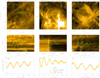 |
Fig. 1. Measurements and fittings of the three selected coronal loops. The columns, from left to right, represent Loop #1, Loop #2, and Loop #3, respectively. Panels a–c: location of the coronal loop. The green solid line shows the path of the loop. Panels d–f: oscillation profiles. The green filled dots are the sampling points of the oscillation profile. Panels g–i: fitting results. The red points with error bars are the aforementioned data points, the blue solid line is the fitting model and the orange region is the confidence band of 95%. |
Physical parameters of the selected coronal loops.
Here, Loop #1 represents the loop oscillation event that occurred at 19:05–19:35 UT on 2010 October 16 and was triggered by a GOES M2.9-class flare (Aschwanden & Schrijver 2011; Kumar et al. 2013); Loop #2 represents the loop oscillation event that occurred at 22:20–22:35 UT on 2011 September 6 and was triggered by a GOES X2.1-class flare (Verwichte et al. 2013); and Loop #3 represents the loop oscillation event that occurred at 1:10–1:50 UT on 2012 March 7 and was triggered by a GOES X5.4-class flare. The 171 Å images of these loops observed by the Atmospheric Imaging Assembly (AIA) on board SDO are shown in Figs. 1a–c. We analyse the base difference movies, in which the first frame is subtracted from other frames, and find that all the loops present characteristic transversal oscillations, whose oscillation profiles are shown in Figs. 1d–f. Regarding the parameter errors listed in Table 1, the Monte Carlo method was used to randomly sow points within the error range of each data point, and statistical standard deviations through 100 times fitting were used to represent the error bar. It should be noted here that although two of the three chosen cases have been studied by other colleagues, our methods for measuring magnetic field are not exactly the same, and the geometry of the coronal loop is taken into account in our work. On the other hand, we also have a new scientific target, which is to measure the physical parameters of the coronal loops and then use a forward modelling method to solve the oscillation period.
Figure 1d shows that Loop #1 is a decayless oscillation (τ1 = ∞), which was explained by Kumar et al. (2013) as being due to successive impacts of a fast-mode wave and a slower ‘EIT wave’. Considering the uncertainties, the fitting period 382.7 ± 2.6 s is consistent with the result of 373 ± 30 s derived by Aschwanden & Schrijver (2011). Also, for Loop #2, the fitted period 148.9 ± 1.3 s is consistent with 150 ± 5 s obtained by Verwichte et al. (2013) within the uncertainty range. In particular, to the best of our knowledge, the oscillation parameters of Loop #3 have not yet been analysed.
These oscillation parameters, especially the oscillation period, are sufficient to decipher average physical quantities such as the magnetic field strength of the loop (Roberts et al. 1984; Andries et al. 2009; Morton et al. 2011). Generally, the loop length can be obtained easily, and the density can be measured using the DEM analysis (Sect. 2.2), although the density is often simplified and considered to be constant along a coronal loop. The average magnetic field strength can then be derived with the assumption ε = ne/ni = 0.1. Furthermore, if the periods of the high-order overtones are measured, we can obtain further information in addition to the average magnetic field strength, such as density scale height (Andries et al. 2005; Van Doorsselaere et al. 2007), which can describe the variation of the density rather than an average quantity.
2.2. Density diagnostics using DEM analysis
DEM analysis is used for temperature and density diagnostics (Aschwanden et al. 2013). Several algorithms have been proposed and their effectiveness has been validated (Weber et al. 2004; Hannah & Kontar 2012; Aschwanden et al. 2013; Plowman et al. 2013; Cheung et al. 2015; Su et al. 2018). Here, we adopt the Oriented Coronal CUrved Loop Tracing (OCCULT) code and the single Gaussian forward fitting method proposed by Aschwanden et al. (2013) to detect the loop segment and then perform the DEM analysis for temperature and density diagnostics. We fit the intensity profiles along the slices in all six extreme-ultraviolet (EUV) passbands from SDO/AIA using a Gaussian function plus a linear background profile to obtain the background-subtracted EUV fluxes,  . With the single-Gaussian DEM fitting, we then derive the peak emission measure, EMi, peak temperature Ti, and the Gaussian temperature width, σT. Accordingly, the electron density, ni, is computed as follows (Aschwanden & Schrijver 2011; Aschwanden et al. 2013; Verwichte et al. 2013; Guo et al. 2015; Dai et al. 2021)
 (2)
(2)
Here, the index i denotes the value measured inside the coronal loop,  is the loop width, and σw is the Gaussian loop width fitted along the cross-sectional profiles.
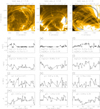 |
Fig. 2. Loop tracing and DEM analysis of the three selected loops. The columns from left to right show the results of Loop #1, Loop #2, and Loop #3, respectively. Panels a–c: loop geometry (dashed line) and their widths (solid line) in 171 Å images. Panels d–f: temperature distribution along the loop geometry. Panels g–i: density distribution along the loop geometry. Panels j–l: width variation along the loop geometry. Panels m–o: goodness of the fitting. |
The results of DEM analysis are shown in Fig. 2. Figures 2d–l depicts the distributions of the temperature Ti, density ni, and loop width w along the three oscillating loops. It can be seen that the maximum amplitudes of the kink oscillation (Figs. 1g–i) are comparable to the width of the loops shown in Figs. 2j–l, which reflects the rationality of the approximation of minor amplitude and the linearisation of MHD equations. The goodness of the fitting is shown in Figs. 2m–o, which indicates that the fitting results are acceptable. It is worth noting that the OCCULT method (Aschwanden et al. 2013) cannot identify the loop as a whole with the complicated EUV backgrounds. Therefore, we sample the loop coordinates interactively with an interactive data language (IDL) code before using the SSW program aia_loop_autodem.pro to obtain the final results.
According to the DEM analysis results shown in Fig. 2, we find that the average temperatures of Loops #1, #2, #3 are 1.07, 0.89, 1.66 MK, respectively. These are typical coronal temperatures (Aschwanden et al. 2013). The temperature distributions of the three studied loops are nearly isothermal as shown in Figs. 2d–f. Besides, the average electron density of the three loops is ni = 0.43 × 10⁹, 0.75 × 10⁹, and 1.12 × 109 cm−3, respectively. Although the density distribution profile is noisy due to line-of-sight (LOS) interference, the trends that the footpoint has higher density and the apex point has a lower density can be seen, which indicates decreasing density with altitude. However, the density distribution in the middle of Fig. 2i is abnormally high, indicating the possible existence of background threads. In Sect. 2.3, the density variation with height is fitted by a function that decays exponentially with loop height:
![Mathematical equation: $$ \begin{aligned} n_\mathrm{i} (s) = n_\mathrm{f} \exp \left[-\dfrac{h(s)}{H}\right], \end{aligned} $$](/articles/aa/full_html/2022/08/aa42711-21/aa42711-21-eq5.gif) (3)
(3)
where H is the density scale height, nf is the density at the footpoint, and h(s) is the height along the loop, which represents the loop geometry. The loop length and the height variation h(s) along the loop are obtained by 3D reconstruction of coronal loops with magnetic field extrapolation in Sect. 2.3.
2.3. 3D magnetic field reconstruction using magnetic field extrapolation
In this section, we show how we processed the HMI data with the 180° ambiguity being removed in the HMI pipeline. In addition to the pipeline process, we corrected the projection effect by a rotation matrix ℛ(P, B, B0, L, L0) (Gary & Hagyard 1990; Guo et al. 2017), which corrects both the vector directions and the geometry. The boundary conditions for potential magnetic field extrapolation were then prepared by a preprocess program, which makes the boundary conditions force-free and torque-free, and extracted the radial magnetic field from the vector magnetic field. Finally, we adopt the potential magnetic field extrapolation algorithm in the Message Passing Interface Adaptive Mesh Refinement Versatile Advection Code (MPI-AMRVAC; Keppens et al. 2003; Porth et al. 2014; Xia et al. 2018). The extrapolated magnetic field is shown in Figs. 3a–c with the SDO/AIA 171 Å images as the background. With the potential field model, the loop length, L, is calculated by integrating the length of magnetic field lines; the height and magnetic field strength distribution along the loop, h(s) and B(s), are obtained (shown in Figs. 3d–f); and the apex heights of the three loops, ha, are found by seeking the maximum of the modified height. For the definition of the modified height, we randomly choose three points in each loop to determine the loop plane and compute its normal vector, that is, the direction cosine αi, βi, γi (the subscript i denotes the index of each loop). We then apply a rotation matrix to convert it to the vertical direction. The dashed lines in Figs. 3d–f represent the average magnetic field calculated by
 (4)
(4)
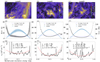 |
Fig. 3. Reconstructed coronal loops and the distribution of their physical parameters. Panels a–c: 3D structure of the magnetic field from a potential field model with the background of the 171 Å waveband on 2010 October 16, 2011 September 6, and 2012 March 7, respectively. Panels d–f: corresponding height (black filled dot), the distribution of the magnetic field strength (blue filled dot) along the loop length, and the average magnetic field strength (blue dashed line). Panels g–i: corresponding electron density (black solid line) and the fitting curve (red dashed line). |
In addition, using the results of the DEM analysis employed, the density scale height and the footpoint density are fitted with Eq. (3) and shown in Figs. 3g–i. Accordingly, an average magnetic field is estimated using the solar magneto-seismological method, which is given by (Roberts et al. 1984)
 (5)
(5)
where we adopt ne/ni = 0.1 as an empirical density ratio between external and internal plasma (Nakariakov et al. 1999; Nakariakov & Ofman 2001), Pkink is P1 as shown in Table 1, mp = 1.67 × 10⁻²⁴ g is the proton mass, and μ = 1.2 is the average molecular weight with the consideration of the coronal abundance. We list the results of Bkink and ⟨B⟩ in Table 1 and find that the magnetic field strength derived by SMS and magnetic field extrapolation is consistent within the range of errors. This reflects the rationality of these two independent approaches to compute the magnetic field. However, other studies reveal a coronal magnetic field exceeding the results of traditional SMS by one or two orders of magnitude, which do not match ours. For example, Vourlidas et al. (2006) and Brosius & White (2006) found a coronal magnetic field of several kilogauss by studying the polarisation of radio emission. Other authors have detected a coronal magnetic field of a few hundred to thousands of Gauss using spectropolarimetry(Schad et al. 2016; Kuridze et al. 2019) and microwave spectral fitting (Chen et al. 2020a,b).
The magnetic field extrapolation matches the coronal loops well, as displayed in Figs. 3a–c, which show that the extrapolated geometric structure and the observed results (in the 171 Å waveband) coincide approximately, except Loop #1 in Fig. 3a. One reason for the misalignment in this case is that this loop is not in an active region and its magnetic field is much weaker than that of the other two cases, as listed in Table 1. Therefore, the precise position of its footpoint is difficult to locate in the magnetogram, which may cause primary errors for our measurement of L, h(s), and B(s). In addition, our solar magneto-seismological result is similar to that of Aschwanden & Schrijver (2011), while our magnetic field extrapolation method is more elaborate because we corrected the projection effect due to the solar spherical surface and located the footpoint with stereoscopic information, both of which were not considered in this latter study. As shown in Fig. 3d, the apex magnetic field Bapex ≈ 3 G seems more acceptable than 6 G in Aschwanden & Schrijver (2011). This is because (1) we obtained ⟨B⟩=4.3 ± 0.1 G and Bkink = 3.9 ± 0.4 G, which are close to each other; but in Aschwanden & Schrijver (2011), ⟨B⟩=11 G is much larger than Bkink = 4.0 ± 0.7 G; and (2) it is reasonable that we had Bapex = 2.8 ± 1.03 G < Bkink = 3.9 ± 0.4 G while it is contradictory that Bapex = 6 G > Bkink = 4.0 ± 0.7 G in Aschwanden & Schrijver (2011).
Subsequently, we reconstructed the geometry (shape of the loop axis and height) of the coronal loop by extrapolating a potential-field model as shown in Figs. 3d–f. As projection correction of the magnetic field involves both vector direction correction and geometric correction, the shape of the coronal loop reconstructed here is not affected by projection effects. For the loop geometry, we use the interpolation function of the height distribution along the loop, h(s), instead of its semi-circular shape h(s)=Lsin(πs/L)/π. It is worth noting that the interpolation function, h(s), is an irregular profile but is closer to the real morphology of the coronal loop. In Fig. 3e, the profile of Loop #2 deviates from a semi-circle, and therefore the traditional model with a semi-circular approximation would not work well in computing the oscillation periods. In contrast, our model would perform well, as discussed in Sect. 3. For the inclination, Verth et al. (2008) mentioned that the neglected inclination leads to a small overestimation factor of 1–2. In our cases, the inclination of the three loops is different. Nevertheless, we assume them to be vertical with the aforementioned operation, which is equivalent to introducing a modified density scale height to remove the effect of inclination. We also assume a planar coronal loop, which is feasible in most cases. In our research, such an approximation is reasonable, except for in the case of Loop #3. As revealed in Fig. 3c, Loop #3 shows an obvious pitch of helix. However, this effect is negligible (Scott & Ruderman 2012), which can be seen in our later results.
Figures 3g–i shows the density profiles fitted by Eq. (3). The density scale heights H of these three coronal loops are listed in Table 1. The apex heights of the loops, ha, as shown in Table 1 are derived by taking the maximum of the height profile (Figs. 3d–f), which is approximately equal to L/π. The density stratification is characterised by ha/H, which is 0.54 ± 0.09 for Loop #1 and 1.09 ± 0.04 for Loop #3. For Loop #2, we find ha/H = 1.57 ± 0.06, which is different from the results of Verwichte et al. (2013), who showed ha/H = 0.985 for the same case. The apex height of Loop #2 determined with the STEREO-A/EUVI 171 Å images by Verwichte et al. (2013) is almost the same as the value reconstructed by the potential field model, demonstrating the validity of the geometry information obtained in our 3D magnetic field model. Also, the magnetic field strength was derived from the potential field source surface (PFSS) model in Verwichte et al. (2013), which is similar to our results from the potential field model. The discrepancy in the density scale height between our work and this latter study is attributed to the fitting of the footpoint density. We use a footpoint density of nf = 17.4 × 108 cm−3 whereas Verwichte et al. (2013) use nf = 7 × 108 cm−3. Figures 3d–i shows that the density distribution and magnetic field strength distribution have a similar decreasing tendency. The density decrease is due to the gravity stratification, ni(h) ∝ e−h/H, in hydrostatic equilibrium. The magnetic field attenuation is due to the dipole potential field, B(h)=B0(1 + h/hd)−3, which decays with height (Erdélyi & Verth 2007). However, Schad et al. (2016) found a case where B0 = 29380 G with spectropolarimetric inversions, which infer a loop magnetic field with strength far beyond the dipole field approximation.
The force-free field models have relatively simple solutions and their magnetic tension and pressure forces balance each other exactly. However, they are too simple to describe the real observation with complex magnetic structures, especially for the more limited potential field models. More importantly, boundary and initial conditions are not accurate enough for observations and more physics should be included in dynamic cases. With all these disadvantages, the potential field model is chosen because it agrees better with observations than the NLFFF model, and is more affordable than dynamic models.
3. String model and comparison to observations
3.1. String model
In order to derive a formula to relate the oscillation period to the coronal loop parameters, we use the analogy of a string to represent the oscillating coronal loop instead of solving the full MHD equations. Figure 4 shows the physical approximation of the string model; an inhomogeneous string that deviates from its equilibrium position after being disturbed. Considering that the coronal loop is actually a magnetic flux tube, if a plasma element P0 deviates from its equilibrium position, it will be subjected to a restoring force due to the elastic nature of the magnetic field line (Fig. 4). Because of the condition of low plasma-β (the ratio of the gas pressure to the magnetic pressure), we only take the magnetic pressure into account and ignore the thermal pressure. Accordingly, the force applying on P0 in the magnetic field of the coronal loop can be expressed as
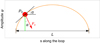 |
Fig. 4. Cartoon of the string model. The red clump P0 represents a reference plasma element deviating from its equilibrium position. The red arrow indicates the magnetic tension force Fc acting on P0, which is directed to the centre of curvature. The direction of Fc makes an angle of α with the vertical direction. |
 (6)
(6)
where μ0 is the permeability of vacuum, j is the current density, and B is the magnetic induction intensity. The first term on the right-hand side of Eq. (6) represents the magnetic pressure gradient. The second term represents the magnetic tension force. It is the magnetic tension force that makes a magnetic field line behave like a string. We decompose the magnetic tension force term in the orthogonal natural coordinate system, which is an orthogonal curvilinear coordinate system with Lamé coefficients of 1:
 (7)
(7)
where  and
and  are the unit vector along the magnetic field and the normal unit vector, respectively. In addition, we use the relation
  and the formula of the analytic geometry
  , where Rc is the radius of curvature of the magnetic field line. Eventually, we find that the force exerted on the plasma P0 is
 (8)
(8)
The second term on the right-hand side of Eq. (8) exactly cancels out the effect of magnetic pressure gradient in the direction of the magnetic field. According to the equilibrium conditions, the magnetic pressure in other directions should also be balanced by the external pressure. The ultimate restoring force, accordingly, is the first term on the right-hand side of Eq. (8), which points to the centre of the curvature and has the effect of pulling the plasma back to its equilibrium position.
We consider a plasma element P0 from s to s + ds; the force along the magnetic field line is at balance, and so the restoring force is normal to the field line. Adding an external magnetic pressure gradient, the total restoring force becomes
 (9)
(9)
where we assume  and define the pressure perturbation
  . Therefore, the momentum equation of the plasma element is
 (10)
(10)
where ψ is the displacement from an equilibrium position, ρ(s) is the distribution of density along the coronal loop, and Rc is the radius of the curvature given by
 (11)
(11)
Here ψs = ∂ψ/∂s, ψss = ∂2ψ/∂s2, with the approximate relation cosα ≈ 1, ψs = tanα ≈ α ≪ 1. We now come up to the equation of coronal loop oscillations:
 (12)
(12)
Alternatively, using the velocity u = ∂ψ/∂t instead of ψ, we have
 (13)
(13)
where vA = B(μ0ρ)−1/2 is the Alfvén speed. According to the fact that the magnetic tension disturbance propagates at the Alvén speed, P satisfies the following wave equation:
 (14)
(14)
where ∇2 is the Laplace operator. With Fourier analysis and the tube boundary condition, the governing equation can be obtained by the combination of Eqs. (13) and (14) (Dymova & Ruderman 2005; Erdélyi & Verth 2007):
 (15)
(15)
where ![Mathematical equation: $ c_\mathrm{k}^2=2B^2[\mu_0(\rho_\mathrm{i}+\rho_\mathrm{e})]^{-1} $](/articles/aa/full_html/2022/08/aa42711-21/aa42711-21-eq24.gif) is the kink mode speed.
is the kink mode speed.
Equation (15) is the governing equation of coronal loop oscillations. Here we use a simplified string model to derive it instead of solving the MHD equations, which helps us to build up a physical picture for understanding coronal loop oscillations. Now that we have such a specific physical picture, we can discuss the damping mechanism and other issues in later follow-up works.
3.2. Analytical solution under a linear loop geometry
Under a number of approximations and assumptions, an analytical solution to the governing equation (Eq. (15)) can be found. Erdélyi & Verth (2007) derived three sets of analytical solutions for a step-function density profile, a linear density profile, and a hyperbolic cosine density profile, respectively. Here, we derive another meaningful solution with an exponential density profile, which corresponds to the case where the coronal loop is approximated as two segments of straight lines as shown as the dash-dotted lines in Fig. 5. Compared with other density profiles, an exponential profile is the simplest case with physical meaning, and so it is also of great value for our discussion.
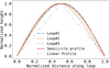 |
Fig. 5. Different geometries of the coronal loop. The purple dash-dot-dotted line and red solid line represent the linear and semi-circular loop geometry, respectively. The blue dash-dotted line, orange dashed line, and green dotted line represent the real loop geometry of Loops #1, #2, and #3, respectively. The apex positions of the real loops slightly deviate from the midpoint (x = 0.5), and the profiles of the coronal loops match the semi-circle loop geometry well. |
For the linear loop geometry without magnetic field variation, its geometric parameters meet the relationship
 (16)
(16)
where ha is the apex height of the coronal loop. Let us take the midpoint of the loop as the origin, that is, s = 0; here s is from −L/2 ≤ s ≤ L/2. By substituting Eq. (16) into Eq. (3), the density distribution can be obtained:
![Mathematical equation: $$ \begin{aligned} n_\mathrm{i} (s) = n_\mathrm{a} \exp \left[\dfrac{|s|}{H} \dfrac{2h_\mathrm{a} }{L} \right]\equiv n_\mathrm{a} \mathrm{e} ^{|s|/H_{L}}. \end{aligned} $$](/articles/aa/full_html/2022/08/aa42711-21/aa42711-21-eq26.gif) (17)
(17)
Here na = nfexp(−ha/H) is the density at the apex. For simplicity, we define a new scale height HL = HL/2ha. As expected, a loop with a linear loop geometry would have an exponential density distribution. Substituting the density profile into the governing Eq. (15) and considering the boundary condition u = 0 at s = ±L/2, we have
 (18)
(18)
where the density ratio ε = ne/ni is a constant. Considering the symmetry or antisymmetry, we consider the right half-segment of the coronal loop, that is, s > 0. Here, we introduce a new variable  ; then Eq. (18) is reduced to
 (19)
(19)
This is the Bessel equation of order zero, and therefore the solution to it is
 (20)
(20)
Considering the boundary condition u(±L/2)=0, we derive the eigenfrequencies
 (21)
(21)
where  represents the nth zero of the Bessel function of order zero. On the other hand, the solution needs to be physical, which requires the continuity of the eigenfunction and its derivative. There are two situations: (1) in the case of odd parity, we supplement the boundary condition u(0)=0; (2) in the case of even parity, we have u′(0)=0. In particular, the supplementary boundary conditions are as follows:
 (22)
(22)
where J1 is the Bessel function of order one. The eigenvalues satisfying the supplementary boundary conditions, Eq. (22), and the intrinsic boundary condition, u(±L/2)=0, will be the subsets of Eq. (21), that is,
 (23)
(23)
Here ns is the integer which meets both Eq. (22) and the intrinsic boundary. The overtone period concerned is then
 (24)
(24)
where vA, f = B(μ0ρf)−1/2 is the Alfvén speed at the footpoint of the coronal loop.
In general, it is difficult to satisfy both Eq. (22) and u(−L/2)=u(L/2)=0 simultaneously. This means that there is usually no physical solution satisfying the intrinsic boundary conditions. Despite this, we can use the solution that best meets the odd or even parity condition as the approximation of the eigenfunctions. The supplementary boundary condition serves as a filter. This approximation means that different L and H will pick out different μns. For instance, Fig. 6 reveals the numerical and analytical solution in the case  s, HL = L. Ignoring the discontinuity of the analytical solution and its first derivative, the eigenvalues and their profiles are close to the numerical one. The period ratio P1/P2 = ω2/ω1 = 1.72 < 2 for the analytical solution and P1/P2 = 1.92 < 2 for the numerical solution both show that the density stratification results in a period ratio of less than 2, implying that the analytical solution is reasonable to a certain extent.
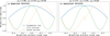 |
Fig. 6. Numerical versus analytical solutions for the linear loop geometry, uniform magnetic field, and stratified density profile. (a) Numerical results of Eq. (18). The blue solid line represents the solution of fundamental tone with eigenvalue ω1 = 2.90, the orange dotted line indicates the first overtone with eigenvalue ω2 = 5.57, and the green dashed line denotes the second overtone with eigenvalue ω3 = 8.54, respectively. (b) Analytical results. The blue solid line represents the solution of fundamental tone with eigenvalue ω1 = 3.37, the orange dotted line indicates the first overtone with eigenvalue ω2 = 5.81, and the green dashed line denotes the second overtone with eigenvalue ω3 = 8.26. Here, we choose |
Equation (24) offers the overtone period of a coronal loop with linear loop geometry and uniform magnetic field. This result shows the following properties qualitatively. First,  , which corresponds to Eq. (5), and
  , which is derived under the approximation of uniform density distribution (Roberts et al. 1984). In addition, Eq. (24) also shows the influence of the density variation, namely, Pn ∝ H/ha, which is the density stratification of the coronal loop (a loop with a semi-circle profile has the density stratification πH/L). It is reasonable that for two coronal loops, where the magnetic field, the shape of the loop axes, and the density of the footpoint are the same except for the density scale height, the loop with the larger density scale height will have a longer period, because less density variation means more inertia. If Eq. (24) gives the same result as Eq. (5) in the example of Fig. 6, then H/ha = 2.75, which means a weak stratification and a nearly uniform density distribution. However, the analytic solution is unreasonable in some sense. This is probably because the simplified model takes many assumptions. One possible unreasonable result is that the period ratio P1/P2 is discrete, which contradicts the previous works where P1/P2 was found to be a continuous function of the density stratification L/πH (Andries et al. 2005; Goossens et al. 2006). Nevertheless, as the results given by Eqs. (24) and (5) differ by only a factor related to density stratification πH/μ1sha, Eq. (24) is valuable when we want to quickly estimate the period of the fundamental tone with the density stratification taken into account.
3.3. Calculating the fundamental period with shooting method
For actual cases, the coronal loop geometry deviates from the linear loop geometry assumed by the analytical solution above. If the real path is considered, the density distribution (Eq. (3)) is so complicated that an analytical solution is unattainable. We need to adopt a numerical method to calculate the period in actual situations. In this section, combining the density, height, and magnetic field distribution obtained from the DEM analysis and magnetic model, we use the shooting method to solve the governing equation to derive the period, and compare it with the period obtained from previous observations and fitting.
For convenience in the numerical solution, we introduce the characteristic length L, time L/vA, f, and magnetic field strength Bav in order to define the dimensionless quantities y = u(s)/vA, f, x = s/L, b = B/Bav, and τ = (2π/ω)/(L/vA, f). The governing equation is non-dimensionalised, which reads
 (25)
(25)
where h(x) is the profile of the coronal loop. Let us take the left footpoint of the loop as the origin where x = 0 and the range of x is from x = 0 to x = 1. If we use a semi-circle profile to approximate a coronal loop, h(x) is expressed as
 (26)
(26)
More precisely, we can describe the real loop geometry using the interpolation function h(x) of the height distribution of the extrapolated magnetic field. The normalized loop geometries are shown in Fig. 5. We can see that in the three coronal loop oscillation events, the actual loop geometries of those loops do not deviate very much from the semi-circular shape.
Here we use the shooting method to solve the boundary value problem in Eq. (25). In detail, we use Wolfram Mathematica to build an interactive window to adjust the period parameters to find the approximate period as the initial value of the shooting method. Then, in the vicinity of a given initial value, we use a seeking algorithm to obtain the final oscillation period satisfying the boundary conditions. The final results are shown in Table 2, in which the observed values Pobs, analytical solutions Panl, numerical solutions with the semi-circle loop geometry Psc, and the numerical solutions with the real loop geometry Preal are compared. The deviation from Pobs is provided in the parentheses following the calculated periods. The accuracy of these three periods increases progressively. More specifically, Preal is the closest to Pobs and their average deviation is 10.6%. The deviation of Psc, 18.3%, is slightly larger than this latter and the deviation of Panl is the largest at 39.3%. This indicates that the eigenvalues of the governing equation are sensitive to the coronal loop geometry.
Period of the fundamental tone.
4. Discussion and conclusions
In this paper, we process three randomly selected coronal loop oscillation events, where the oscillation periods of the coronal loops are fitted. In all three events, only the fundamental tone is detected, and there is no obvious higher overtone component. We estimate the density distribution of the coronal loop using DEM diagnostics, and then we use the exponential decay model to fit the density scale height. Next, we use the potential field model to extrapolate the magnetic field distribution of the coronal loop, and thereby reconstruct the 3D structure of the loops. This analysis led us to three important results, as follows.
-
Combining the information available on the density and oscillations, we estimate an average magnitude of the magnetic field strength of Bkink = 3.9 ± 0.4, 24.9 ± 0.8, and 14.4 ± 0.5 G for the three events considered. These values are consistent with the results derived by applying the magnetic field extrapolation ⟨B⟩=4.3 ± 0.1, 22.9 ± 0.1, and 16.0 ± 0.1 G, respectively.
-
We used a string model to derive the approximated governing equation of the coronal loop and find an analytic solution (Eq. (24)) under the assumption that the loop has a linear loop geometry, exponentially stratified density, and uniform magnetic field. This solution requires a correction factor πH/μ1sha to Eq. (5) when taking the influence of the density variation into account. It is shown that a loop with higher density scale height H has a longer period, as expected.
-
We used both analytical and numerical methods to compute the periods with the information of density, magnetic field, and different loop geometries. The periods calculated with the extrapolated loop geometries are closest to the observed ones, which are better than those periods calculated with the loop geometry taken as a semi-circle or a linear shape.
There are several uncertainties in our calculations and some improvement can be made in future, which is discussed from the aspects of oscillation analysis, DEM diagnostics, assumptions in the calculations, and magnetic field extrapolation as follows.
In our oscillation analysis, we sampled the data within a certain time window and the non-linear fitting model is incomplete, which would cause some errors in deriving the oscillation parameters. In fact, we also tried to measure the oscillation period using spectral analysis methods such as discrete Fourier transform and wavelet transform. However, due to the fact that we sampled the data in a certain time window, the frequency detected by the former method is limited in resolution, which means that the period value cannot be obtained accurately. On the other hand, the wavelet transform depends on the choice of a suitable wavelet function. While it is more effective to use spectral analysis to confirm the existence of higher order overtones, it is more precise to acquire the period of the fundamental frequency using a fitting method.
The density and temperature distributions are diagnosed with the DEM analysis in Sect. 2.2, where the density distributions are obtained with the SSW routine aia_loop_autodem.pro. To have the density of the entire loop, we sampled the data manually. As a DEM analysis needs to satisfy the assumption of optical thickness and relies on the integration along the LOS, the final temperature diagnostics has a large error and will affect the density measurement through error transmission. In addition, if the starting and ending points of our sampling data are not consistent with the actual footpoints of the coronal loop, the density distribution will affect the fitting results of the density scale height H and the density at the footpoint nf.
It is worth noting that the coronal loop structure obtained in our simulation has an inclination and the loop geometry deviates from a semi-circle, which were taken into account in our calculations. We selected three points at a coronal loop to determine the loop plane, and then the influence of the inclination was eliminated by using the rotation matrix to rotate it to the vertical direction. Next, the profile of the coronal loop was represented by an interpolation function of the height distribution along the loop. Finally, the two complicated factors, the inclination and loop geometry, were considered in the governing equations. The results show that the coronal loop geometry has a significant influence on the periods (Table 2). A loop with different paths and the same magnetic and density distribution would have markedly different oscillation periods.
In our measurement of Loop #1 (as shown in Fig. 3), the magnetic field Bkink derived using the solar magneto-seismological method is 3.9 ± 0.4 G while Aschwanden & Schrijver (2011) obtained Bkink = 4.0 ± 0.7 G. We adopted ε = 0.1 which is close to ε = 0.08 ± 0.01 used in Aschwanden & Schrijver (2011). However, our derived plasma density ni = 4.3 × 108 cm−3 is larger than ni = (1.9 ± 0.3) × 108 cm−3 obtained in Aschwanden & Schrijver (2011), and the loop length L = 96.1 ± 10.98 Mm in our measurement is much smaller than Losc = 143 ± 20 Mm used in Aschwanden & Schrijver (2011). We integrated the length of the selected field lines as the coronal loop length, whereas Aschwanden & Schrijver (2011) adopted the trigonometric method. Our loop length is sensitive to the accuracy of the magnetic model, and there is some considerable error as indicated by the mismatch between the simulated magnetic field and the observed coronal loops (see Fig. 3a). The average magnetic field strength ⟨B⟩=4.3 ± 0.10 G obtained via Eq. (4) is much lower than ⟨B⟩=11 G derived by Aschwanden & Schrijver (2011). Here, we used the magnetic field extrapolation derived by the potential field model, which is more accurate on small scales than the PFSS model applied in Aschwanden & Schrijver (2011). This is because the PFSS method makes use of the synoptic map of the SDO/HMI magnetogram, which is constructed from the observations during a whole rotation. As a result, the magnetic field obtained by the PFSS method is less accurate than the magnetic field extrapolation using the real-time magnetogram. However, our magnetic field extrapolation in the Cartesian coordinates adopts the linear approximation using a plane tangent to the solar surface at the image centre (Gary & Hagyard 1990). This would cause deviations near the solar limb or with a relatively large field of view. The aforementioned error can be eliminated with the extrapolation in the spherical coordinate (Gilchrist & Wheatland 2014; Guo et al. 2016a,b).
In conclusion, in the three chosen coronal loop oscillation events, we measured the density distribution with a DEM analysis and obtained the distribution of magnetic field strength as well as the information on loop geometry with magnetic field extrapolations. We then used the physical and geometrical parameters to compute the oscillation periods, which deviate from the observed values by only 10.6% on average. That is to say, the period derived by considering the realistic density, magnetic field, and loop geometry comprehensively coincides with the observed period. In addition, our multi-tool research shows that the loop geometry significantly affects the oscillation properties of coronal loops, which indicates that the period is sensitive not only to the density and magnetic field but also to the loop geometry.
Acknowledgments
The SDO data are available by courtesy of NASA/SDO and the AIA and HMI science teams. This research was supported by NSFC (11773016, 11733003, 11533005, and 11961131002), National Key Research and Development Program of China (2020YFC2201200). R.E. is grateful to Science and Technology Facilities Council (STFC grant No. ST/M000826/1) UK for the financial support.
References
- Andries, J., Arregui, I., & Goossens, M. 2005, ApJ, 624, L57 [NASA ADS] [CrossRef] [Google Scholar]
- Andries, J., van Doorsselaere, T., Roberts, B., et al. 2009, Space Sci. Rev., 149, 3 [Google Scholar]
- Aschwanden, M. J., & Schrijver, C. J. 2011, ApJ, 736, 102 [NASA ADS] [CrossRef] [Google Scholar]
- Aschwanden, M. J., Fletcher, L., Schrijver, C. J., & Alexander, D. 1999, ApJ, 520, 880 [Google Scholar]
- Aschwanden, M. J., de Pontieu, B., Schrijver, C. J., & Title, A. M. 2002, Sol. Phys., 206, 99 [CrossRef] [Google Scholar]
- Aschwanden, M. J., Boerner, P., Schrijver, C. J., & Malanushenko, A. 2013, Sol. Phys., 283, 5 [NASA ADS] [CrossRef] [Google Scholar]
- Brosius, J. W., & White, S. M. 2006, ApJ, 641, L69 [NASA ADS] [CrossRef] [Google Scholar]
- Chen, B., Shen, C., Gary, D. E., et al. 2020a, Nat. Astron., 4, 1140 [Google Scholar]
- Chen, B., Yu, S., Reeves, K. K., & Gary, D. E. 2020b, ApJ, 895, L50 [NASA ADS] [CrossRef] [Google Scholar]
- Cheung, M. C. M., Boerner, P., Schrijver, C. J., et al. 2015, ApJ, 807, 143 [Google Scholar]
- Chiu, Y. T., & Hilton, H. H. 1977, ApJ, 212, 873 [NASA ADS] [CrossRef] [Google Scholar]
- Dai, J., Zhang, Q. M., Su, Y. N., & Ji, H. S. 2021, A&A, 646, A12 [NASA ADS] [CrossRef] [EDP Sciences] [Google Scholar]
- Duckenfield, T., Anfinogentov, S. A., Pascoe, D. J., & Nakariakov, V. M. 2018, ApJ, 854, L5 [Google Scholar]
- Duckenfield, T. J., Goddard, C. R., Pascoe, D. J., & Nakariakov, V. M. 2019, A&A, 632, A64 [NASA ADS] [CrossRef] [EDP Sciences] [Google Scholar]
- Dymova, M. V., & Ruderman, M. S. 2005, Sol. Phys., 229, 79 [Google Scholar]
- Erdélyi, R., & Taroyan, Y. 2008, A&A, 489, L49 [NASA ADS] [CrossRef] [EDP Sciences] [Google Scholar]
- Erdélyi, R., & Verth, G. 2007, A&A, 462, 743 [NASA ADS] [CrossRef] [EDP Sciences] [Google Scholar]
- Gary, G. A., & Hagyard, M. J. 1990, Sol. Phys., 126, 21 [Google Scholar]
- Gilchrist, S. A., & Wheatland, M. S. 2014, Sol. Phys., 289, 1153 [NASA ADS] [CrossRef] [Google Scholar]
- Goossens, M., Andries, J., & Arregui, I. 2006, Phil. Trans. R. Soc. London, Ser. A, 364, 433 [Google Scholar]
- Guo, Y., Erdélyi, R., Srivastava, A. K., et al. 2015, ApJ, 799, 151 [NASA ADS] [CrossRef] [Google Scholar]
- Guo, Y., Xia, C., & Keppens, R. 2016a, ApJ, 828, 83 [NASA ADS] [CrossRef] [Google Scholar]
- Guo, Y., Xia, C., Keppens, R., & Valori, G. 2016b, ApJ, 828, 82 [NASA ADS] [CrossRef] [Google Scholar]
- Guo, Y., Cheng, X., & Ding, M. 2017, Sci. China Earth Sci., 60, 1408 [Google Scholar]
- Hannah, I. G., & Kontar, E. P. 2012, A&A, 539, A146 [NASA ADS] [CrossRef] [EDP Sciences] [Google Scholar]
- Keppens, R., Nool, M., Tóth, G., & Goedbloed, J. P. 2003, Comput. Phys. Commun., 153, 317 [Google Scholar]
- Kumar, P., Cho, K. S., Chen, P. F., Bong, S. C., & Park, S.-H. 2013, Sol. Phys., 282, 523 [NASA ADS] [CrossRef] [Google Scholar]
- Kuridze, D., Mathioudakis, M., Morgan, H., et al. 2019, ApJ, 874, 126 [Google Scholar]
- Li, H., Liu, Y., & Vai Tam, K. 2017, ApJ, 842, 99 [NASA ADS] [CrossRef] [Google Scholar]
- Morton, R. J., & Erdélyi, R. 2010, A&A, 519, A43 [NASA ADS] [CrossRef] [EDP Sciences] [Google Scholar]
- Morton, R. J., Ruderman, M. S., & Erdélyi, R. 2011, A&A, 534, A27 [NASA ADS] [CrossRef] [EDP Sciences] [Google Scholar]
- Nakariakov, V. M., & Ofman, L. 2001, A&A, 372, L53 [NASA ADS] [CrossRef] [EDP Sciences] [Google Scholar]
- Nakariakov, V. M., Ofman, L., Deluca, E. E., Roberts, B., & Davila, J. M. 1999, Science, 285, 862 [Google Scholar]
- Newkirk, G., & Altschuler, M. 1969, BAAS, 1, 288 [NASA ADS] [Google Scholar]
- Pascoe, D. J., Goddard, C. R., & Nakariakov, V. M. 2016, A&A, 593, A53 [NASA ADS] [CrossRef] [EDP Sciences] [Google Scholar]
- Pesnell, W. D., Thompson, B. J., & Chamberlin, P. C. 2012, Sol. Phys., 275, 3 [Google Scholar]
- Plowman, J., Kankelborg, C., & Martens, P. 2013, ApJ, 771, 2 [NASA ADS] [CrossRef] [Google Scholar]
- Porth, O., Xia, C., Hendrix, T., Moschou, S. P., & Keppens, R. 2014, ApJS, 214, 4 [Google Scholar]
- Roberts, B., Edwin, P. M., & Benz, A. O. 1984, ApJ, 279, 857 [CrossRef] [Google Scholar]
- Ruderman, M. S., & Erdélyi, R. 2009, Space Sci. Rev., 149, 199 [Google Scholar]
- Ruderman, M. S., Shukhobodskiy, A. A., & Erdélyi, R. 2017, A&A, 602, A50 [NASA ADS] [CrossRef] [EDP Sciences] [Google Scholar]
- Schad, T. A., Penn, M. J., Lin, H., & Judge, P. G. 2016, ApJ, 833, 5 [Google Scholar]
- Schatten, K. H., Wilcox, J. M., & Ness, N. F. 1969, Sol. Phys., 6, 442 [Google Scholar]
- Schmidt, H. U. 1964, On the Observable Effects of Magnetic Energy Storage and Release Connected With Solar Flares, 50, 107 [Google Scholar]
- Schrijver, C. J., & De Rosa, M. L. 2003, Sol. Phys., 212, 165 [Google Scholar]
- Schrijver, C. J., Title, A. M., Berger, T. E., et al. 1999, Sol. Phys., 187, 261 [NASA ADS] [CrossRef] [Google Scholar]
- Schrijver, C. J., Aschwanden, M. J., & Title, A. M. 2002, Sol. Phys., 206, 69 [Google Scholar]
- Scott, A., & Ruderman, M. S. 2012, Sol. Phys., 278, 177 [NASA ADS] [CrossRef] [Google Scholar]
- Seehafer, N. 1978, Sol. Phys., 58, 215 [NASA ADS] [CrossRef] [Google Scholar]
- Su, Y., Veronig, A. M., Hannah, I. G., et al. 2018, ApJ, 856, L17 [NASA ADS] [CrossRef] [Google Scholar]
- Tomczyk, S., McIntosh, S. W., Keil, S. L., et al. 2007, Science, 317, 1192 [Google Scholar]
- Van Doorsselaere, T., Nakariakov, V. M., & Verwichte, E. 2007, A&A, 473, 959 [NASA ADS] [CrossRef] [EDP Sciences] [Google Scholar]
- Verth, G., Erdélyi, R., & Jess, D. B. 2008, ApJ, 687, L45 [NASA ADS] [CrossRef] [Google Scholar]
- Verwichte, E., Nakariakov, V. M., Ofman, L., & Deluca, E. E. 2004, Sol. Phys., 223, 77 [Google Scholar]
- Verwichte, E., Van Doorsselaere, T., Foullon, C., & White, R. S. 2013, ApJ, 767, 16 [Google Scholar]
- Vourlidas, A., Gary, D. E., & Shibasaki, K. 2006, PASJ, 58, 11 [NASA ADS] [CrossRef] [Google Scholar]
- Weber, M. A., Deluca, E. E., Golub, L., & Sette, A. L. 2004, in Multi-Wavelength Investigations of Solar Activity, eds. A. V. Stepanov, E. E. Benevolenskaya, & A. G. Kosovichev, 223, 321 [NASA ADS] [Google Scholar]
- Xia, C., Teunissen, J., El Mellah, I., Chané, E., & Keppens, R. 2018, ApJS, 234, 30 [Google Scholar]
All Tables
All Figures
|
Fig. 1. Measurements and fittings of the three selected coronal loops. The columns, from left to right, represent Loop #1, Loop #2, and Loop #3, respectively. Panels a–c: location of the coronal loop. The green solid line shows the path of the loop. Panels d–f: oscillation profiles. The green filled dots are the sampling points of the oscillation profile. Panels g–i: fitting results. The red points with error bars are the aforementioned data points, the blue solid line is the fitting model and the orange region is the confidence band of 95%. |
| In the text | |
|
Fig. 2. Loop tracing and DEM analysis of the three selected loops. The columns from left to right show the results of Loop #1, Loop #2, and Loop #3, respectively. Panels a–c: loop geometry (dashed line) and their widths (solid line) in 171 Å images. Panels d–f: temperature distribution along the loop geometry. Panels g–i: density distribution along the loop geometry. Panels j–l: width variation along the loop geometry. Panels m–o: goodness of the fitting. |
| In the text | |
|
Fig. 3. Reconstructed coronal loops and the distribution of their physical parameters. Panels a–c: 3D structure of the magnetic field from a potential field model with the background of the 171 Å waveband on 2010 October 16, 2011 September 6, and 2012 March 7, respectively. Panels d–f: corresponding height (black filled dot), the distribution of the magnetic field strength (blue filled dot) along the loop length, and the average magnetic field strength (blue dashed line). Panels g–i: corresponding electron density (black solid line) and the fitting curve (red dashed line). |
| In the text | |
|
Fig. 4. Cartoon of the string model. The red clump P0 represents a reference plasma element deviating from its equilibrium position. The red arrow indicates the magnetic tension force Fc acting on P0, which is directed to the centre of curvature. The direction of Fc makes an angle of α with the vertical direction. |
| In the text | |
|
Fig. 5. Different geometries of the coronal loop. The purple dash-dot-dotted line and red solid line represent the linear and semi-circular loop geometry, respectively. The blue dash-dotted line, orange dashed line, and green dotted line represent the real loop geometry of Loops #1, #2, and #3, respectively. The apex positions of the real loops slightly deviate from the midpoint (x = 0.5), and the profiles of the coronal loops match the semi-circle loop geometry well. |
| In the text | |
|
Fig. 6. Numerical versus analytical solutions for the linear loop geometry, uniform magnetic field, and stratified density profile. (a) Numerical results of Eq. (18). The blue solid line represents the solution of fundamental tone with eigenvalue ω1 = 2.90, the orange dotted line indicates the first overtone with eigenvalue ω2 = 5.57, and the green dashed line denotes the second overtone with eigenvalue ω3 = 8.54, respectively. (b) Analytical results. The blue solid line represents the solution of fundamental tone with eigenvalue ω1 = 3.37, the orange dotted line indicates the first overtone with eigenvalue ω2 = 5.81, and the green dashed line denotes the second overtone with eigenvalue ω3 = 8.26. Here, we choose |
| In the text | |
Current usage metrics show cumulative count of Article Views (full-text article views including HTML views, PDF and ePub downloads, according to the available data) and Abstracts Views on Vision4Press platform.
Data correspond to usage on the plateform after 2015. The current usage metrics is available 48-96 hours after online publication and is updated daily on week days.
Initial download of the metrics may take a while.