| Issue |
A&A
Volume 678, October 2023
|
|
|---|---|---|
| Article Number | A205 | |
| Number of page(s) | 12 | |
| Section | The Sun and the Heliosphere | |
| DOI | https://doi.org/10.1051/0004-6361/202346393 | |
| Published online | 24 October 2023 | |
Measuring local physical parameters in coronal loops with spatial seismology
1
School of Astronomy and Space Science and Key Laboratory for Modern Astronomy and Astrophysics, Nanjing University, 163 Xianlin Avenue, Qixia District, Nanjing 210023, PR China
e-mail: This email address is being protected from spambots. You need JavaScript enabled to view it.
; This email address is being protected from spambots. You need JavaScript enabled to view it.
2
Solar Physics and Space Plasma Research Center (SP2RC), School of Mathematics and Statistics, University of Sheffield, Hicks Building, Hounsfield Road, Sheffield S3 7RH, UK
3
Department of Astronomy, Eötvös Lorand University, Pázmány Péter sétány 1/A, Budapest 1117, Hungary
4
Gyula Bay Zoltan Solar Observatory (GSO), Hungarian Solar Physics Foundation (HSPF), Petőfi tér 3., Gyula 5700, Hungary
Received:
13
March
2023
Accepted:
4
September
2023
Abstract
Context. The method of spatial seismology can be applied to the amplitude profile of transverse coronal loop oscillations to constrain the distributions of physical parameters, such as the loop density, magnitude of the magnetic field, and so on.
Aims. We intend to develop and apply a practical spatial seismology technique to detect physical parameters of plasma and validate its effectiveness by comparing it with other methods.
Methods. A spatial seismology inversion was conducted by numerically optimizing a parametric dynamic model of the loop’s density stratification and magnetic field variation to best fit the measured amplitude profile of the loop.
Results. The spatial seismology inversion technique developed here was applied to a transverse coronal loop oscillation that occurred on 2013 April 11, whose oscillation amplitude profile of both the fundamental mode and first overtone was reported in previous work. The consistency between the time domain analysis and spatial seismology has been verified. Meanwhile, we accounted for the asymmetric profile of the fundamental mode by forward modeling and we derived the magnetic field distribution by inverse modeling, which is coincident with that of the extrapolated one. In addition, spatial seismology inversion was applied to the transverse oscillation event on 2022 March 30 to obtain the distribution of the loop’s density and magnetic field, which are compared with the results derived from the differential emission measure (DEM) diagnostics and the direct potential field extrapolation.
Conclusions. Spatial seismology inversion can be used as an effective method to independently measure various physical parameters, for example the density and magnetic field of coronal loops, which are consistent with the results obtained by DEM diagnostics and potential field extrapolation.
Key words: Sun: corona / Sun: magnetic fields / Sun: oscillations
© The Authors 2023
 Open Access article, published by EDP Sciences, under the terms of the Creative Commons Attribution License (https://creativecommons.org/licenses/by/4.0), which permits unrestricted use, distribution, and reproduction in any medium, provided the original work is properly cited.
This article is published in open access under the Subscribe to Open model. This email address is being protected from spambots. You need JavaScript enabled to view it. to support open access publication.
1. Introduction
Physical parameters such as the magnetic field and density are vital factors that allow for the eruptions and atmospheric fluctuations on the Sun to be determined. Therefore, measuring the local physical plasma parameters on the Sun is a focal topic in solar physics research. Solar magneto-seismology (SMS) is a method to determine these key physical parameters by, for example, standing and/or propagating waves (Roberts et al. 1984). The transverse coronal loop oscillations triggered by an occasional solar eruption are usually used in SMS (Aschwanden et al. 1999; Schrijver et al. 1999), because of its remarkable characteristics in observations and its strong dependence on plasma density and the magnetic field. For a review, readers can refer to Ruderman & Erdélyi (2009).
Specifically, SMS tries to measure oscillation periods of the fundamental mode of kink waves to calculate the average Alfvén speed and then the average magnetic field (Roberts et al. 1984; Aschwanden & Schrijver 2011). The average magnetic field can also be measured by radio observations of the brightness temperature of the third-order gyroresonance emission (Vourlidas et al. 2006). However, when it comes to measuring the distribution of the magnetic field, conventional seismology that is limited to temporal domain analysis is challenging. Commonly used methods to estimate the magnetic field distribution include magnetic field extrapolations (Verwichte et al. 2013; Guo et al. 2015; Erdélyi et al. 2022), spectropolarimetric inversions (Schad et al. 2016), and some other complicated and cumbersome procedures. As a typical extrapolation method, the potential field model computes the vector magnetic field by extrapolating the normal magnetic field from the photosphere observed by, for example, the Helioseismic and Magnetic Imager (HMI; Scherrer et al. 2012; Schou et al. 2012) using the Green’s function method, for instance. Meanwhile, with spectropolarimetry one inverts the vector magnetic field by numerically optimizing a parametric radiation transfer model to best fit observed Stokes spectra (Lagg et al. 2004; Lagg 2007; Schad et al. 2016), which is one of the most accurate methods for a direct magnetic field measurement. As for other physical parameters, differential emission measure (DEM) diagnostics provides estimates of the density and temperature along the loop (Weber et al. 2004; Hannah & Kontar 2012; Aschwanden et al. 2013; Plowman et al. 2013; Cheung et al. 2015; Su et al. 2018). On the other hand, the SMS method could also employ the period ratio of the fundamental mode and the first overtone of the transverse oscillation to determine the density scale height (Andries et al. 2005a,b, 2009a; Arregui et al. 2005; Goossens et al. 2006; Dymova & Ruderman 2006; Van Doorsselaere et al. 2007; Verth et al. 2007; Ruderman et al. 2008). Furthermore, the electron density can be derived from the intensity ratio of two Fe XIII lines at 1074.7 and 1079.8 nm. Then, combined with the phase speed measured by a wave-tracking technique, the magnetic field on the plane of sky can be obtained (Yang et al. 2020a,b). In addition to the density stratification along the loop axis, the density stratification across the axis also affects the eigenvalues and may produce damping (Arregui et al. 2005; Dymova & Ruderman 2006).
It can be seen that the temporal domain SMS has no theoretical advantages when compared with other methods in measuring the density and magnetic field, and it has some obvious limitations. First, it is difficult for the temporal domain SMS to determine the magnetic field distribution, while only the average magnetic field can be obtained with the fundamental mode. Second, it depends on the detection of the first or higher order overtone to derive more information about the physical parameters. In fact, the detection about overtone depends on the spectral analysis of, for example, the wavelet transform (Verwichte et al. 2004; Duckenfield et al. 2019) or the oscillation profile fitting (Aschwanden & Schrijver 2011; Verwichte et al. 2013; Guo et al. 2015). However, it is difficult to detect a measurable signal of an overtone for most of the coronal loop oscillations. In fact, most of them have no obvious visible overtone components. Third, the temporal domain SMS is based on the assumption that a coronal loop is symmetric in both geometry and magnetic field properties, while the coronal loops in reality are most likely symmetric in geometry (close to a semicircular loop path) but asymmetric in magnetic field distribution. The temporal domain SMS has a limited ability to diagnose the asymmetric physical properties of the coronal loops.
However, if applying SMS in the spatial domain rather than in the temporal domain, the above limitations can be removed up to a large degree. The governing equation of transverse loop oscillations is a Sturm-Liouville problem for the differential equation of second-order on a finite interval with Dirichlet boundary conditions (Dymova & Ruderman 2005). The temporal domain SMS is only based on the eigenvalues of the governing equation, while the spatial domain SMS, called spatial seismology, attempts to take advantage of its eigenfunctions, which have a certain distribution and can provide more constraints on the physical parameters than the pure eigenvalues. Erdélyi & Verth (2007) found three sets of analytic solutions for the governing equation using the assumption of three different density profiles, respectively, and analyzed the numerical solution of the fundamental tone. Verth et al. (2007) numerically exhibited that the antinode of the first overtone shifts toward the footpoints with the density scale height decreasing, which implies that the density scale height depends on the distribution of the overtone amplitudes. In addition, it has been reported that the shift of the first overtone’s antinode can be used to estimate the magnetic expansion factor Γ = ra/rf, where ra and rf are the minus radii of the loop at the apex and footpoint, respectively (Verth et al. 2008). Additionally, under an approximation of a thin magnetic slab embedded in a nonmagnetic weakly asymmetric environment, the magnetic field strength could be approximately determined with the relative amplitude difference of the sausage mode between the two sides of the slab (see Oxley et al. 2020). Zsámberger & Erdélyi (2022) subsequently generalized this model to an asymmetric magnetic environment and proposed the amplitude ratio technique and the minimum perturbation shift technique for spatial seismology. All of the above theories are the foundation for seismology in the spatial domain and reveal the feasibility of spatial seismology. As for observations, the amplitude profile of a transverse oscillation, which occurred on 2001 September 15 and was observed by the Transition Region And Coronal Explorer (TRACE), was first reported by Verwichte et al. (2010).
For this work, we developed a spatial seismology technique, which allows asymmetric distributions of the physical parameters. Our intention was to detect the magnetic field and density of coronal loops by means of spatial seismology and compare the results with DEM diagnostics and potential field extrapolation. The paper is organized as follows: the inversion, based on spatial seismology, is introduced in Sect. 2. The effectiveness of spatial seismology inversion has been validated by applying the method to two specific events, as explained in Sect. 3, and the conclusion and discussion are in Sect. 4
2. Theory and method
The governing equation of transverse coronal loop oscillations can be derived from linearizing the magnetohydrodynamic (MHD) equations and one thus obtains (Dymova & Ruderman 2005, Eq. (21))
 (1)
(1)
where ![Mathematical equation: $ c_{\rm k}^2 = 2B^2[\mu_0(\rho_\mathrm{i}+\rho_\mathrm{e})]^{-1} $](/articles/aa/full_html/2023/10/aa46393-23/aa46393-23-eq2.gif) is the kink mode speed, and ρi and ρe are the internal and external density, respectively. This equation was derived using the assumption of a straight flux tube. Here, the variable u denotes the radial velocity along the tube. Equation (1) was expressed with a mathematical proxy Q, which was constructed mathematically and proportional to u in Dymova & Ruderman (2005). The successful application of the seismology in spatial domain depends on solving Eq. (1). However, it is not easy to solve Eq. (1) analytically, which requires some assumptions and model simplifications. Erdélyi & Verth (2007) solved the governing equation as examples to demonstrate the power of the method, and under the assumption that the density profiles are a step function, a linear function, or a hyperbolic cosine function. Chen et al. (2022) also found an analytic solution of a coronal loop with a linear geometric profile. In spatial seismology it is easier to proceed with numerical rather than analytical solutions to the governing equation. Therefore, Eq. (1) can be rewritten in a dimensionless form as (Chen et al. 2022)
is the kink mode speed, and ρi and ρe are the internal and external density, respectively. This equation was derived using the assumption of a straight flux tube. Here, the variable u denotes the radial velocity along the tube. Equation (1) was expressed with a mathematical proxy Q, which was constructed mathematically and proportional to u in Dymova & Ruderman (2005). The successful application of the seismology in spatial domain depends on solving Eq. (1). However, it is not easy to solve Eq. (1) analytically, which requires some assumptions and model simplifications. Erdélyi & Verth (2007) solved the governing equation as examples to demonstrate the power of the method, and under the assumption that the density profiles are a step function, a linear function, or a hyperbolic cosine function. Chen et al. (2022) also found an analytic solution of a coronal loop with a linear geometric profile. In spatial seismology it is easier to proceed with numerical rather than analytical solutions to the governing equation. Therefore, Eq. (1) can be rewritten in a dimensionless form as (Chen et al. 2022)
 (2)
(2)
which is convenient to be solved numerically. Here, τ = (2π/ω)/(L/vA, f) is the dimensionless period, and ε = ρe/ρi is the ratio between the external and internal density, with an empirical value of 0.1 (Nakariakov & Ofman 2001). The parameter x = s/L is the normalized distance along the loop, y = u/vA, f is the dimensionless velocity, and φ(x) = (n(x)/nc)(B(x)/Bc)−2 depends on the distribution function of the density and magnetic field along the loop, where nc and Bc are the chosen characteristic density and magnetic field, respectively. For instance, for a loop with a semicircular axis, uniform magnitude for the magnetic field, B(x) = B0, and an exponentially decaying density stratification, ne = n0 ⋅ exp[ − (L/πH)sin(πx)], we have φ(x) = exp[ − (L/πH)⋅sin(πx)]; whereas, for a loop with a uniform density, ρ = ρ0, and a dipole magnetic field B = B0(1 + h/D)−3 (Aschwanden 2005; Erdélyi & Verth 2007), we have φ(x) = [1 + (L/πD)⋅sin(πx)]6. We note that H and D denote the density scale height and the embedding depth of the magnetic charge, respectively. The former ϕ(x) can be used to solve for the eigenvalues of the governing equation dominated by density stratification, to determine the density scale height L/πH, and to explain the observational result of P1/P2 < 2 (reported in Duckenfield et al. 2018; Guo et al. 2015), as shown in Fig. 1a (also refer to Andries et al. 2005a). It must be pointed out that we neglected the stratification across the loop axis, that is, the effect of a transitional layer, which can actually also cause damping and changes of periods (Ruderman & Petrukhin 2022).
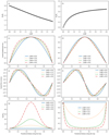 |
Fig. 1. Effect of density stratification and the magnetic field variation on the period ratio P1/P2 and on the eigen functions of both the fundamental mode and the first overtone. Panel a: period ratio varying with L/πH. Panel b: similar to panel a, but with L/πD. Panel c: amplitude profiles of the fundamental mode for different values of L/πH, denoted by different line styles. Panel d: similar to panel c, but for different values of L/πD. Panel e: amplitude profiles of the first overtone for different values of L/πH. Panel f: similar to panel e, but for different values of L/πD. Panel g: Alfvén speed distribution for different L/πH. Panel h: similar to panel g, but for different L/πD. In panels a,c,e, we fixed L/πD = 0 to ensure that eigenmodes and eigenvalues are only affected by the density variation, and in panels b,d,f, we fixed L/πH = 0. |
On the other hand, Fig. 1b reveals how the period ratio P1/P2 varies with the magnetic field. We note that the effect of magnetic field variation is opposite to that of density stratification on the period ratio and can be used to explain the observational result of P1/P2 > 2 (De Moortel & Brady 2007; Pascoe et al. 2016). One interpretation is that  , and thus the magnetic field variation plays an opposite effect when compared with that of density stratification. Figures 1g,h exhibit the Alfvén speed distribution along the loop in different L/πH or L/πD, where
  is a characteristic speed. The local Alfvén speed appears to be a decisive quantity for the oscillation property. For the kink mode oscillation, the phase speed is associated with the Alfvén speed (Roberts et al. 1984). Thus the distribution of VA determines the eigenvalues of the oscillation and then the eigen modes.
Here, we adopted the dipole field to solve the governing equation. The dipole field model approximates the measured magnetic field of the coronal loop well (Schad et al. 2016), and the dipole model only introduces one free parameter, the embedding depth D of the magnetic charge, to describe the magnetic field distribution. The impact of the magnetic field on P1/P2 can also be explained by the tube expansion (Ruderman et al. 2008; Verth et al. 2008). In the first order approximation, the period ratio reads as
![Mathematical equation: $$ \begin{aligned} \dfrac{P_1}{P_2} = 2\left[1+\dfrac{3(\Gamma ^2-1)}{2\pi ^2}\right]. \end{aligned} $$](/articles/aa/full_html/2023/10/aa46393-23/aa46393-23-eq6.gif) (3)
(3)
Here, Γ = ra/rf is the expansion factor. It is reasonably expected that the tube expansion and the magnetic field variation have similar effects on the period ratio. In the case of flux conservation, the flux tube expansion is caused by the attenuation of the magnetic field with loop height. Therefore, employing flux conservation  , we then obtain Γ = (1 + L/πD)1.5. It must be pointed out that the eigenvalues depend on both density stratification and flux tube expansion. Here, we only discuss the impact of the tube expansion.
Figures 1c–f exhibit the eigenfunctions (amplitude profiles) of the fundamental mode and the first overtone dominated by density stratification and magnetic field variation, respectively. Specifically, Figs. 1c and e show the effect of density stratification on the fundamental mode and the first overtone, corresponding to φ(x) = exp[ − (L/πH)⋅sin(πx)] in Eq. (2). Figures 1d and f denote the effect of magnetic field variation, corresponding to φ(x) = [1 + (L/πD)⋅sin(πx)]6. For the fundamental mode, density stratification broadens the eigenfunction, while the magnetic field variation narrows it. In the case of a larger L/πH, the apex is relatively thinner while the footpoints of the loop are relatively denser, which results in a greater amplitude due to more inertia near the footpoints. However, a larger L/πD means a stronger field at the footpoints, where the amplitude should be smaller since the magnetic field offers a restoring force during the oscillation. For the first overtone, its antinode shifts toward the footpoints when density stratification is dominant, while it departs from the footpoints when the magnetic field variation is dominant (Verth 2007; Verth et al. 2008). One qualitative explanation is that the density provides inertia but the magnetic field provides a restoring force, and thus a strong magnetic field at the footpoints can push the antinodes toward the center while the density has the opposite effect. It must be pointed out that the results in Fig. 1e are the same as those in Verth et al. (2007, 2008). We redrew it in order to emphasize the impact of different physical parameters on the eigenmode, leading to spatial seismology accordingly. Verth et al. (2007) found a good linear approximation between the normalized antinode shift and the density scale height,
 (4)
(4)
In addition, the antinode shift can also be used to estimate the tube expansion by the relation (Verth et al. 2008; Andries et al. 2009b)
 (5)
(5)
where |ΔzAN| is the shift displacement of the first overtone’s left (right) antinode from the regular position of 0.25L (0.75L). Both density stratification and flux tube expansion contribute to the position of the antinode shift, as shown in Figs. 1e and f. Both the density and magnetic stratifications may take effect concurrently, and therefore it may be hard to separate one from the other. However, if we find that the antinodes shift toward both footpoints, we may assume that density stratification is dominant, in which case the density scale height can be estimated using Eq. (4). On the contrary, if the antinodes become closer to the midpoint of the loop, we may assume that the flux tube expansion is dominant and the expansion factor Γ can be estimated by Eq. (5).
However, a first overtone is often hard to detect, let alone performing measurements of its amplitude profile and the position of the antinode. On the contrary, the fundamental mode can be measured for many transversely oscillating coronal loops, and thus it is easier to obtain the amplitude profile along the loop of the fundamental tone than the first overtone. Therefore, in order to consider the feasibility of spatial seismology, the fundamental mode should be investigated.
We consider a simple case with just one parameter in which the magnetic field is constant and the density exponentially decays with a density scale height H. This assumption was employed by Andries et al. (2005a) to solve the eigenvalues of the governing equation. By numerically solving Eq. (2) with φ(x) = exp[ − (L/πH)⋅sin(πx)] using the shooting method, we obtained the normalized amplitude distribution map of the fundamental mode against L/πH, as shown in Fig. 2.
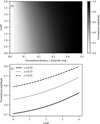 |
Fig. 2. Normalized amplitude distribution map of the fundamental mode. Panel a: 2D plot of the normalized amplitude of the fundamental mode with varying L/πH and x. When fixing a certain L/πH, one can get an amplitude profile of the fundamental mode along the loop. Panel b: normalized amplitude of the fundamental mode against the L/πH at different positions on the loop. |
When we measured the amplitude of the fundamental mode at a certain position of the coronal loop; the result in Fig. 2 can be used to determine the magnitudes with different L/πH. For illustration purposes, we plotted the normalized amplitude of the fundamental mode against L/πH at x = 0.1, 0.15 , and 0.20 (Fig. 2b), which is a monotonic function. As seismology in the temporal domain determines L/πH by the monotonic function of P1/P2 against L/πH (Fig. 1a), in applying spatial seismology, one can do that using a normalized amplitude distribution (Fig. 2). Furthermore, applying the temporal seismology using the period ratio provides only one constraint; whereas, in using spatial seismology, the estimated amplitude at each location along the waveguide can provide a constraint. Therefore, all the measured data can be used to determine the density scale height by numerically minimizing a parameter of χ2.
In addition, spatial seismology can implement multi-parameter regression, because the amplitude measured at each position provides a constraint. In detail, the density and magnetic field distributions can be taken into account by adding more relative parameters to φ(x; k1, k2, …) in Eq. (2), where k1, k2, … are the undetermined coefficients associated with the physical parameters of plasma. For instance, we could consider both of the density and magnetic field variations with a double parameter φ(x) (see Sect. 3.2), and we could also consider an asymmetric distribution of the magnetic field by adding an extra parameter in φ(x) (see Sect. 3.1). Then, we substituted φ(x; k1, k2, …) into Eq. (2) and numerically solved the equation by the shooting method to obtain the fundamental mode ψ(x; k1, k2, …), which depends on k1, k2, … as well.
Comparing it with the measured amplitude profile, the data points {xi, ηi}, where i = 1, 2, …, and the fitting goodness χ2 could be computed,
 (6)
(6)
where N is the number of the measurement of the amplitude, and the coefficient c with a dimension of Mm−1 was used to convert the measured amplitude ηi to the normalized one. With an optimization algorithm such as simulated annealing, the relative parameters, k1, k2, …, can be eventually determined. Since the degree of freedom of χ2 is N − 1, and an undetermined parameter c is introduced in Eq. (6), at least two more amplitude values than the number of free parameters are required. In fact, because of the errors in the amplitude measurement, in order to make a strong constraint, we needed to measure as many amplitudes as possible.
To summarize, spatial seismology uses a combination of coronal loop oscillation observations, the governing equation of coronal loop oscillations, and the optimization algorithm of simulated annealing to determine the magnetic field and density in coronal loops (Fig. 3). This method has a number of advantages over temporal seismology. The seismology in the temporal domain relies on, for example, the measurement of the first overtone, which is hard to obtain. However, spatial seismology only requires the distribution of the fundamental mode, which can be obtained relatively easily for all coronal loop oscillations. In addition, it is the eigenvalue of the governing equation, or the period, that is considered when making use of seismology in the temporal domain, while the eigenfunction is taken into account when implementing spatial seismology. The former can provide only one constraint, while the latter can provide several. Therefore, by applying spatial seismology, one can invert the parameters form the given physical models. Last but not least, the asymmetric distribution can be derived from spatial seismology but cannot be done by temporal domain seismology because too few constrains are provided in the latter.
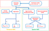 |
Fig. 3. Flow chart of SMS. The green boxed region exhibits the spatial SMS inversion and the yellow boxed region illustrates how the temporal SMS determines the physical parameters. |
3. Application to observations
In this section, we explain how we applied spatial seismology to observations in order to analyze the density and magnetic field and verify the consistency between the modeling results and the measurements.
3.1. Oscillation on 2013 April 11
A coronal loop was disturbed by an M6.5 class flare on 2011 April 11 and a characteristic transverse oscillation was triggered. Guo et al. (2015) detected both the fundamental mode and first overtone for this event, with periods of 519.9 ± 55.3 s and 334.7 ± 22.1 s, respectively. The measured period ratio is P1/P2 = 1.55 ± 0.19, where the error 0.19 was derived from the error transfer formula. The reason why the period ratio deviates from two is a result of multiple factors, such as the finite tube width and curvature (McEwan et al. 2006), density stratification (Andries et al. 2005a,b; McEwan et al. 2006), and the magnetic field variation along the loop (Verth et al. 2008). A period ratio less than two may suggest that density stratification plays a major role in the oscillation. In addition, the amplitude profiles of the fundamental mode and first overtone were also measured. The first overtone’s profile is too noisy to provide accurate information. However, it is fortunate that the amplitude of the fundamental mode could be measured at seven locations in the southern part of the coronal loop. The fundamental mode shows an asymmetric feature, where the amplitude peak shifts to the southern footpoint, which is different from the theoretical result in Fig. 1c. Since the observed oscillation has revealed both temporal and spatial information, we suggest carrying out three studies:
-
To verify the consistency of the seismology results in the temporal and spatial domains,
-
To obtain the eigenfunction (amplitude profile) of the fundamental mode by a forward modeling method and explain the observed asymmetry of the amplitude profile, and
-
To invert the magnetic field distribution by spatial seismology and compare the results with the extrapolated field based on the potential field model.
First of all, according to P1/P2 = 1.55 ± 0.19 and the relation shown in Fig. 1a, we find that ![Mathematical equation: $ L/\pi H = 2.28^{+0.98}_{-0.82}\in [1.43,3.62] $](/articles/aa/full_html/2023/10/aa46393-23/aa46393-23-eq11.gif) . The difference between the upper and lower errors is due to the nonlinear relation of L/πH against P1/P2. According to the seven sets of the amplitude profile (xi, ηi) of Fig. 6a in Guo et al. (2015), an expression for χ2 with six degrees of freedom (DOF) can be written as follows:
. The difference between the upper and lower errors is due to the nonlinear relation of L/πH against P1/P2. According to the seven sets of the amplitude profile (xi, ηi) of Fig. 6a in Guo et al. (2015), an expression for χ2 with six degrees of freedom (DOF) can be written as follows:
 (7)
(7)
For this study, the supplementary parameter c was used to convert a physical amplitude η with the dimension of megametre (Mm) to a scaled amplitude yi = c ⋅ ηi as shown in Fig. 2, and ψ is the eigenfunction of the fundamental tone, derived by solving Eq. (2) with φ(x) = exp[−(L/πH)⋅sin(πx)].
Through a simulated annealing algorithm, we obtained ![Mathematical equation: $ L/\pi H = 1.88^{+1.06}_{-1.04}\in [1.04, 3.94] $](/articles/aa/full_html/2023/10/aa46393-23/aa46393-23-eq13.gif) with
with  and c = 0.22. The error was estimated by sampling the amplitude values within the range of the error bar 100 times to invert the density scale height and then take the maximum and minimum, respectively. The inversion result of L/πH is consistent with the value of
  derived from the temporal domain analysis within the range of errors.
Second, we intended to forwardly fit the amplitude profile by substituting the measured density and magnetic field into the governing equation to account for the asymmetry of the fundamental mode. We adopted the extrapolated magnetic field derived from the potential field model (see Guo et al. 2015, Fig. 6a) and the density scale height L/πH = 2.28 derived from the period ratio. By solving Eq. (2) using the shooting method, the fundamental mode was obtained as shown in Fig. 4a. It can be seen from Fig. 4a that the forward fitting result agrees with the measured amplitude profile in Guo et al. (2015). It must be pointed out that the measured amplitude was multiplied by a coefficient, 0.11 Mm−1, converted to the scaled amplitude. Doing so can minimize the standard deviation between the measured amplitude and the result from the numerical solution. Since only the magnetic field is asymmetric in our parametric model, the asymmetry in the abnormal fundamental model should be caused by the distribution of the magnetic field, which supports the explanation in Guo et al. (2015).
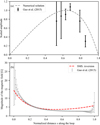 |
Fig. 4. Results of forward fitting and spatial seismology inversion for the oscillation event on 2013 April 11. Panel a: asymmetric fundamental mode derived from forwardly solving the governing equation. The dashed line denotes the numerical solution of the fundamental mode and the solid points with error bars refer to the amplitude profile measured in Guo et al. (2015), multiplied by a coefficient of 0.11 Mm−1. Panel b: comparison of the magnetic field derived from spatial seismology inversion and potential field extrapolation. The red dashed line denotes the inversion result by spatial seismology and the solid points with error bars represent the extrapolated field. |
Finally, using the known physical parameters to calculate the fundamental mode can only illustrate the feasibility of the numerical method to solve the governing equation. In fact, it is of greater value to use the fundamental mode to invert the local unknown physical parameters. Therefore, we took advantage of such a good observational result to invert the magnetic field distribution and compared it with the extrapolated magnetic field to verify its accuracy. Just as we have done when inverting the density scale height, we minimized a new expression of χ2 as defined below,
 (8)
(8)
Here, the parameters L/πD1 and L/πD2 determined the asymmetric distribution of the magnetic field as follows,
![Mathematical equation: $$ \begin{aligned} B_0(x)= {\left\{ \begin{array}{ll} B_0\left[1+\dfrac{L}{\pi D_1}\sin (\pi x)\right]^{-3},&0\le x\le 0.5\\ B_0\left[1+\dfrac{L}{\pi D_2}\sin (\pi x)\right]^{-3}\cdot \left[\dfrac{1+L/\pi D_1}{1+L/\pi D_2}\right]^{-3},&0.5<x\le 1. \end{array}\right.} \end{aligned} $$](/articles/aa/full_html/2023/10/aa46393-23/aa46393-23-eq17.gif) (9)
(9)
Such a constructed magnetic field conforms to an approximate relation for a dipole field, B = B0(1 + h/D)−3, on the left and right halves, respectively. With the magnetic field given as by Eq. (9), we could substitute
![Mathematical equation: $$ \begin{aligned} \varphi (x) = \exp [-(L/\pi H)\cdot \sin (\pi x)]\cdot (B(x)/B_0)^{-2}\nonumber \end{aligned} $$](/articles/aa/full_html/2023/10/aa46393-23/aa46393-23-eq18.gif)
into Eq. (2) to find the amplitude profile of the fundamental mode for different parameters L/πD1 and L/πD2, that is, ψ(L/πD1, L/πD2). Here, we took L/πH = 2.28, derived from the period ratio P1/P2, to reduce the free parameters to two quantities. Because only seven amplitudes were measured, it was complicated to constrain three parameters with χ2 of six DOFs. Then, we found L/πD1 = 0.58 and L/πD2 = 0.17, corresponding to the minimum  , by using the simulated annealing algorithm as well. The inversion result is shown by the red dashed line in Fig. 4b, which is in good agreement with the extrapolated result indicated as the gray points with error bars. It is revealed that spatial seismology inversion can be used as an effective method to obtain the distribution of the magnetic field.
In fact, when we adopted the model that derives the density scale height from the period ratio (Andries et al. 2005a), we could not ignore that it assumes a uniform magnetic field distribution, which contradicts the model used in spatial seismology inversion. We actually attempted to consider L/πH as another free parameter to carry out incersion. When adopting such three free parameters, the inversion result always slides to the boundary of the parameter space, which only provides a trivial result. This is because there are only seven measured amplitudes of the fundamental mode due to the complex extreme-ultraviolet (EUV) background. Further, because of the large errors of the measurements, the constraints are so weak that we have to make a compromise during the parameter inversion. If we consider L/πH as a free parameter, we have four undetermined parameters. Using only six DOFs to constrain four free parameters is too limiting. Therefore, we made a simplification, using the period ratio P1/P2 to fix L/πH, thereby reducing the complexity of the inversion. In fact, when comparing the final inversion results with the observations (Fig. 4), it indicates that our simplification is acceptable.
3.2. Oscillation on 2022 March 30
On 2022 March 30, an X1.3 class flare occurred in AR 12977. The flare started at 17:27 UT, ended at 17:46 UT, and peaked at 17:37 UT, which triggered oscillations of a cluster of coronal loops at (W25.8°, S17.9°), located in the southern direction from the flare epicenter.
Figure 5 shows the full-disk observation of the Sun and the chosen coronal loop in the 171 Å waveband at 17:20 UT, recorded by the Atmospheric Imaging Assembly (AIA; Lemen et al. 2012) on board the Solar Dynamics Observatory (SDO; Pesnell et al. 2012). The loops are oriented from east to west, almost parallel to the equator. We checked the base and running difference movies from 17:20 UT to 18:20 UT and found an obvious transverse oscillation occurring at 17:40 UT. We selected 20 slices along the north-south direction as shown in Fig. 5. Thanks to the specific loop location and its apparent north-south polarization, the oscillation profile can obviously be revealed in the time-distance diagram from slice 6 to slice 20, as plotted in Fig. 6.
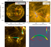 |
Fig. 5. SDO/AIA 171 Å image and the extrapolated magnetic field. Panel a: full-disk image in 171 Å at 17:20 UT. Panel b: subregion of the SDO/AIA image overlaid with the line-of-sight magnetic field observed by SDO/HMI. The loop path is denoted by the green dashed line and the selected slices are marked by the red dashed lines. Panel c: potential field model overlaid on the AIA 171 Å image. Panel d: side view of the reconstructed loop. The red dashed lines show the slice position on the loop and the direction of the line of sight. |
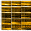 |
Fig. 6. Time-distance diagram for slices 6–20. The image shows the amplitude profiles of the oscillation, triggered at 17:40 UT, along the loop for each slice. The red dashed lines denote the fitting result of a damping cosine profile. |
Figure 6 shows the time-distance diagram of slices 6–20, which excellently reveals the amplitude profile along the loop. As the slice moves from east to west, the amplitude of the oscillations becomes larger. Such a favorable observation in the spatial domain can offer a good opportunity to obtain constraints for spatial seismology analysis. For further study, we used a damping cosine function,
![Mathematical equation: $$ \begin{aligned} A(t)=A_{00}+A_{01}(t-t_0)+A_1\cos \left[\dfrac{2\pi }{P_1}(t-t_0)-\phi _{01}\right]\mathrm{e} ^{-\frac{t-t_0}{\tau _1}}, \end{aligned} $$](/articles/aa/full_html/2023/10/aa46393-23/aa46393-23-eq20.gif) (10)
(10)
to fit the oscillation evolution. Here, A00, A01, A1, t0, τ1, ϕ01, and P1 represent the displacement, linear drift velocity, oscillation amplitude, reference time, damping timescale, initial phase, and fundamental period, respectively. Since we need to use the scaled amplitude ultimately, it is convenient to directly use pixels as the units of amplitude in the fitting instead of megametre (Mm) or arcsec. The fitting curves are denoted in Fig. 6 and the fitting results are listed in Table 1.
Fitting parameters of amplitude profiles.
The oscillation has only a distinct fundamental component and no first overtone can be detected. Therefore, it is sufficient to fit the profile using Eq. (10). Here, we care about the oscillation period and the amplitude distribution. The average period is ⟨P1⟩ = 729.5 ± 47.6 s, where the error was computed as the root mean square of the standard deviation and the error transfer formula. In addition, the amplitudes measured have a tendency to increase with the slice number. This means that we just measured a segment of the loop and the selected slices do not cover the other part since the other half of the loop is not visible in the 171 Å waveband. There is a drawback that measurements are not available for a complete coronal loop because the results of applying seismology in both the temporal domain and spatial domain depend on the measurements of the loop path. The former needs estimates of the geometrical loop length (Roberts et al. 1984; Aschwanden & Schrijver 2011), while the latter needs information about certain locations at which the amplitudes are measured along the loop. The three-dimensional (3D) loop geometry can usually be deduced by applying the triangulation method to stereoscopic observations (Aschwanden & Schrijver 2011), which are observed by, for example, the Solar Terrestrial Relations Observatory (STEREO), or by reconstructing the magnetic field with the potential field model (Guo et al. 2015; Verwichte et al. 2013; Chen et al. 2022). For this work, we also used the potential field extrapolation to reconstruct the 3D structure of the loop for convenience. Doing so has also made it feasible to compare the magnetic field inverted from spatial seismology with the extrapolated one.
We first corrected the projection effect of the magnetic field recorded by HMI using a rotation matrix ℛ(P, B, B0, L, L0) (Gary & Hagyard 1990; Guo et al. 2017). Then, the radial component of the projection-corrected magnetic field was used as the boundary condition for the potential field. Finally, we adopted the Green’s function method to compute the magnetic field by the Message Passing Interface Adaptive Mesh Refinement Versatile Advection Code (MPI-AMRVAC; Keppens et al. 2003, 2023; Porth et al. 2014; Xia et al. 2018). The extrapolated field is represented by the colored tube in Fig. 5c, which is overlapped on the AIA image in 171 Å. It can be seen that the extrapolated field coincides well with the visible segment of the coronal loop, which indicates that it is reasonable to reconstruct the 3D geometry of the loop by the potential field model. The loop length was measured to be 329.9 ± 5.6 Mm. Then, we plotted the slice position on the back-projection image of the magnetic field. Figure 5d shows the side view of the extrapolated filed and the red dashed line denotes the slices’ position and the direction of the line of sight (LOS). According to the reconstructed 3D loop geometry, we plotted the amplitude distribution in Fig. 7d. The selected slices only cover a part of the entire loop, which explains why the measured amplitude increases gradually with the slice number instead of decreasing. In addition, we could also obtain the distribution of the magnetic field strength, as shown in Fig. 7c, which is also asymmetrical.
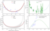 |
Fig. 7. Inversion results of spatial seismology. Panel a: density distribution computed by DEM diagnostics (the blue diamonds), the inversion result of spatial seismology (the red dashed line), and the fitting result to the observed data using an exponentially damping profile (the black dashed line). Panel b: distribution of the measured Alfvén speed (the green star point) and the fitted Alfvén speed (the blue dotted line). Panel c: distribution of the magnetic field strength extrapolated from the potential field model (the gray points with error bars), the inversion result of magnetic field (the red dashed line), the fitting result to the extrapolated field using a bipolar model (the black dashed line). Panel d: measured amplitude multiplied by a scaling coefficient of 0.027 pixel−1 (the blue diamonds with error bars), and the inverted fundamental mode with L/πH = 1.50 and L/πD = 0.61 (the green dotted line). |
In addition, we also performed a DEM analysis to invert the plasma density. Here, we adopted the Oriented Coronal CUrved Loop Tracing (OCCULT) code proposed by Aschwanden et al. (2013) to identify the loop segment. Considering that the OCCULT method cannot identify the loop as a whole, we also relied on the reconstructed loop to determine where the density was measured. We employed a Gaussian profile plus a linear background to fit the intensity variation along the loop radius in all SDO/AIA wavebands to obtain the peak flux,  , and Gaussian loop width σw. The Gaussian width σw could be used to estimate the loop width by
  . The background-subtracted EUV fluxes,
  , could be used for the single Gaussian forward DEM fitting, from which we derived the peak emission measure, EMp, peak temperature, Tp, and the Gaussian temperature width, σT. The density was then computed as
 (11)
(11)
where the subscript i refers to the density inside the coronal loop.
Figure 7a shows the density distribution computed by DEM diagnostics, where the normalized distance x along the loop was derived from finding the corresponding position of the sampling points. It can be seen that the sampling points do not cover the full interval of the normalized distance [0,1], which indicates that the OCCULT algorithm has not identified the coronal loop as a whole. We also checked the temperature distribution and found that the loop is approximately isothermal with Tp = 6.17 MK. With the extrapolated magnetic field and the density from the DEM diagnostics, we exhibit the Alfvén speed distribution in Fig. 7b. The Alfvén speed was computed by  , where mp = 1.67 × 10⁻²⁴ g is the proton mass and μ = 1.2 is the average molecular weight with the consideration of the coronal abundance.
Then, we performed spatial seismology to invert the density and magnetic field distribution. We define the following physical model: the geometry of the loop is a semicircle, the density decays exponentially with the relation ni(x) = nf ⋅ exp[−(L/πH)sin(πx)], and the magnetic field is a bipolar field as B(x) = B0[1 + h(x)/D]−3. Therefore, Eq. (2) could be solved to yield
![Mathematical equation: $$ \begin{aligned} \varphi (x)=\exp [-(L/\pi H)\sin (\pi x)]\cdot [1+(L/\pi D)\cdot \sin (\pi x)]^6.\nonumber \end{aligned} $$](/articles/aa/full_html/2023/10/aa46393-23/aa46393-23-eq26.gif)
The reason why we just used a symmetric bipolar field but not an asymmetric field as expressed by Eq. (9) is that we only measured the amplitudes on the east half of the loop, which cannot offer a good constraint on the information of the asymmetric quantity. We have also checked the inversion results using Eq. (9) and found that the value of the χ2 function has no nontrivial minimum in the given parameter space. Therefore, we adopted a dipole field model for the inversion. Accordingly, we define the following chi-square function as
 (12)
(12)
Here, ψ(x) is the parametric fundamental mode eigenfunction of Eq. (2) with φ(x) mentioned above, ηi is the amplitude measured at xi, and c is the scaling coefficient to ηi. Then, we obtained L/πH = 1.50, L/πD = 0.61, and c = 0.027 pixel−1, which correspond to a minimum  . The density scale height was derived as H = 70.0 ± 1.2 Mm, which is different with that in an isothermal atmosphere H = kT/(μmp g⊙) = 155.2 Mm (g⊙ is the acceleration of gravity on the surface of the Sun). This implies that the existence of the Lorentz force intensifies the density stratification of plasma.
Figure 7 exhibits the inversion results compared with the density distribution obtained by the DEM analysis and the magnetic field distribution derived from the potential field model. As expected, the inversion results from spatial seismology are in good agreement with the measured distribution of the density and magnetic field. It can be seen that the density inverted by spatial seismology matches the density obtained from the DEM analysis relatively well. The inverted magnetic field matches the extrapolated field only on the east side of the loop but it has a large deviation on the west side. Because we could only measure the amplitude of the east half of the coronal loop, there is no information about the asymmetry. For an approximately semi-circular loop, the density distribution should be nearly symmetric; thus, the amplitude measurement for only half a loop is roughly adequate for an inversion. However, in order to reflect the asymmetric properties of the magnetic field, at least the position of the antinode needs to be measured. And we could calculate the inverted Alfvén speed according to the inverted density and magnetic field, whose errors were derived from the error transfer formula (shown in Fig. 7). The inverted Alfvén speed also agrees well with the measured one. In addition, we note that the inverted fundamental mode eigen function matches the measured amplitude distribution well, as can be seen in Fig. 7.
4. Conclusion and discussion
In this paper, we have developed a dynamic inversion method for spatial seismology, which could be used to diagnose the coronal loop oscillations in the spatial domain instead of the temporal domain. We have discussed the influence of density stratification and magnetic field variation on both the eigenvalues and eigenfunctions. Density stratification makes P1/P2 less than two, the fundamental mode amplitude profile becomes wider, and the antinodes of the first overtone shift toward the footpoints. However, the magnetic field variation has the opposite effect. A similar conclusion was also reported in Andries et al. (2005a). By a numerical solution, we obtained the fundamental mode amplitude profile with different values of density scale height L/πH (Fig. 2). We propose that the value of L/πH can be constrained by the measured amplitude at a certain position on the loop. Furthermore, if the amplitudes at different locations are measured to form an amplitude distribution, the physical parameters can be inverted by numerically optimizing the parametric density and magnetic field model to best fit the amplitude profile, which is the inversion by spatial seismology.
Namely, we implemented the spatial seismology technique in two cases, as explored in Sect. 3. The consistency between the seismology in the spatial domain and temporal domain was verified. In both of the cases, we achieved inverting the distribution of the magnetic field and density with the measurement of the amplitude distribution. The effectiveness and feasibility of spatial seismology inversion was validated by comparing the inversion results with the extrapolated magnetic field and the density derived from the DEM diagnostics.
To summarize, the temporal seismology focus on the eigenvalues of the governing equation but spatial seismology focuses on the eigenfunctions (or eigenvectors). Compared with both of them, spatial seismology has the following several advantages.
-
The amplitude measured at each location along the loop can offer a constraint, and thus the amplitude profile along the loop can be applied to invert multiple physical parameters.
-
Applying spatial seismology only requires the amplitude of the fundamental mode at different locations along the loop instead of the higher order overtone. For almost all coronal loop oscillations, their fundamental mode can be easily measured, but only a few of the higher order overtones can be detected.
-
The Rayleigh-Ritz theorem implies that when factors such as the asymmetry is introduced, eigenvectors are more significantly affected (perturbed) than eigenvalues (see Oxley et al. 2020, appendix). Consequently, spatial seismology that focuses on the eigenvectors could have a higher sensitivity on measuring some certain physical parameters.
However, there exist some limitations in spatial seismology. First, although it is easy to measure the amplitudes at different locations along a loop, spatial seismology requires the normalized distance along the loop. Commonly, it is difficult to establish the 3D structure of the whole loop accurately enough. For example, the west half of the coronal loop, discussed in Sect. 3.2, is invisible because of the complex EUV background. Even if we can capture a whole coronal loop, it is still difficult to reconstruct its 3D geometry by triangulation that relies on dual-perspective observations separated by a suitably large angle. Second, spatial seismology is a dynamic inversion method after all. It heavily depends on the parametric model of the density and magnetic field, and thus its accuracy is much lower than that of spectropolarimetric inversions. Third, the local fluctuation of the magnetic field cannot be obtained due to the limitation of the mathematical model. In addition, if there is no clear evolution profile of the loop oscillation or if the measurement error is too large, one may be unable to reach a reasonable fitting result by minimizing χ2.
The above limitation also points to the future development of the spatial seismology inversion technique. For example, it may be possible to improve the accuracy of the inversion by applying a more appropriate χ2, similar to those that involve the errors, to evaluate the inversion results. In addition, we only employed the simplest exponential density stratification and dipole magnetic field here. One may also use a model that considers more comprehensive physical factors and contains more parameters for inversion. In addition, in some special cases, spatial seismology can perhaps be used as a complementary tool to other magnetic field measurements. For instance, if coronal loops are located at or near the limb of the Sun, the potential field extrapolation using the SDO/HMI magnetic field becomes inaccurate due to the projection effects. In such a case, spatial seismology relying on just the dynamic inversion is an alternative method for magnetic field reconstruction.
Acknowledgments
SDO data are available by courtesy of NASA/SDO and the AIA and HMI science teams. This work is supported by the National Key R&D Program of China (2022YFF0503004, 2021YFA1600504, 2020YFC2201201) and NSFC (11773016, 11733003). R.E. is grateful to Science and Technology Facilities Council (STFC grant No. ST/M000826/1) UK and also acknowledges NKFIH (OTKA, grant No. K142987) Hungary for enabling this research.
References
- Andries, J., Arregui, I., & Goossens, M. 2005a, ApJ, 624, L57 [NASA ADS] [CrossRef] [Google Scholar]
- Andries, J., Goossens, M., Hollweg, J. V., Arregui, I., & Van Doorsselaere, T. 2005b, A&A, 430, 1109 [NASA ADS] [CrossRef] [EDP Sciences] [Google Scholar]
- Andries, J., Arregui, I., & Goossens, M. 2009a, A&A, 497, 265 [NASA ADS] [CrossRef] [EDP Sciences] [Google Scholar]
- Andries, J., van Doorsselaere, T., Roberts, B., et al. 2009b, Space. Sci. Rev., 149, 3 [CrossRef] [Google Scholar]
- Arregui, I., Van Doorsselaere, T., Andries, J., Goossens, M., & Kimpe, D. 2005, A&A, 441, 361 [NASA ADS] [CrossRef] [EDP Sciences] [Google Scholar]
- Aschwanden, M. J. 2005, Physics of the Solar Corona. An Introduction with Problems and Solutions (2nd edn.), (Chichester, UK: Praxis Publishing Ltd.) [Google Scholar]
- Aschwanden, M. J., & Schrijver, C. J. 2011, ApJ, 736, 102 [NASA ADS] [CrossRef] [Google Scholar]
- Aschwanden, M. J., Fletcher, L., Schrijver, C. J., & Alexander, D. 1999, ApJ, 520, 880 [Google Scholar]
- Aschwanden, M. J., Boerner, P., Schrijver, C. J., & Malanushenko, A. 2013, Sol. Phys., 283, 5 [NASA ADS] [CrossRef] [Google Scholar]
- Chen, G. Y., Chen, L. Y., Guo, Y., et al. 2022, A&A, 664, A48 [NASA ADS] [CrossRef] [EDP Sciences] [Google Scholar]
- Cheung, M. C. M., Boerner, P., Schrijver, C. J., et al. 2015, ApJ, 807, 143 [Google Scholar]
- De Moortel, I., & Brady, C. S. 2007, ApJ, 664, 1210 [NASA ADS] [CrossRef] [Google Scholar]
- Duckenfield, T., Anfinogentov, S. A., Pascoe, D. J., & Nakariakov, V. M. 2018, ApJ, 854, L5 [Google Scholar]
- Duckenfield, T. J., Goddard, C. R., Pascoe, D. J., & Nakariakov, V. M. 2019, A&A, 632, A64 [NASA ADS] [CrossRef] [EDP Sciences] [Google Scholar]
- Dymova, M. V., & Ruderman, M. S. 2005, Sol. Phys., 229, 79 [Google Scholar]
- Dymova, M. V., & Ruderman, M. S. 2006, A&A, 457, 1059 [NASA ADS] [CrossRef] [EDP Sciences] [Google Scholar]
- Erdélyi, R., & Verth, G. 2007, A&A, 462, 743 [NASA ADS] [CrossRef] [EDP Sciences] [Google Scholar]
- Erdélyi, R., Korsós, M. B., Huang, X., et al. 2022, J. Space Weather Space Clim., 12, 2 [CrossRef] [EDP Sciences] [Google Scholar]
- Gary, G. A., & Hagyard, M. J. 1990, Sol. Phys., 126, 21 [Google Scholar]
- Goossens, M., Andries, J., & Arregui, I. 2006, Phil. Trans. R. Soc. London, Ser. A, 364, 433 [Google Scholar]
- Guo, Y., Erdélyi, R., Srivastava, A. K., et al. 2015, ApJ, 799, 151 [NASA ADS] [CrossRef] [Google Scholar]
- Guo, Y., Cheng, X., & Ding, M. 2017, Science China Earth Sciences, 60, 1408 [NASA ADS] [CrossRef] [Google Scholar]
- Hannah, I. G., & Kontar, E. P. 2012, A&A, 539, A146 [NASA ADS] [CrossRef] [EDP Sciences] [Google Scholar]
- Keppens, R., Nool, M., Tóth, G., & Goedbloed, J. P. 2003, Comput. Phys. Commun., 153, 317 [Google Scholar]
- Keppens, R., Popescu Braileanu, B., Zhou, Y., et al. 2023, A&A, 673, A66 [NASA ADS] [CrossRef] [EDP Sciences] [Google Scholar]
- Lagg, A. 2007, Adv. Space Res., 39, 1734 [Google Scholar]
- Lagg, A., Woch, J., Krupp, N., & Solanki, S. K. 2004, A&A, 414, 1109 [NASA ADS] [CrossRef] [EDP Sciences] [Google Scholar]
- Lemen, J. R., Title, A. M., Akin, D. J., et al. 2012, Sol. Phys., 275, 17 [Google Scholar]
- McEwan, M. P., Donnelly, G. R., Díaz, A. J., & Roberts, B. 2006, A&A, 460, 893 [NASA ADS] [CrossRef] [EDP Sciences] [Google Scholar]
- Nakariakov, V. M., & Ofman, L. 2001, A&A, 372, L53 [NASA ADS] [CrossRef] [EDP Sciences] [Google Scholar]
- Oxley, W., Zsámberger, N. K., & Erdélyi, R. 2020, ApJ, 890, 109 [NASA ADS] [CrossRef] [Google Scholar]
- Pascoe, D. J., Goddard, C. R., & Nakariakov, V. M. 2016, A&A, 593, A53 [NASA ADS] [CrossRef] [EDP Sciences] [Google Scholar]
- Pesnell, W. D., Thompson, B. J., & Chamberlin, P. C. 2012, Sol. Phys., 275, 3 [Google Scholar]
- Plowman, J., Kankelborg, C., & Martens, P. 2013, ApJ, 771, 2 [NASA ADS] [CrossRef] [Google Scholar]
- Porth, O., Xia, C., Hendrix, T., Moschou, S. P., & Keppens, R. 2014, ApJS, 214, 4 [Google Scholar]
- Roberts, B., Edwin, P. M., & Benz, A. O. 1984, ApJ, 279, 857 [CrossRef] [Google Scholar]
- Ruderman, M. S., & Erdélyi, R. 2009, Space. Sci. Rev., 149, 199 [CrossRef] [Google Scholar]
- Ruderman, M. S., & Petrukhin, N. S. 2022, Sol. Phys., 297, 72 [NASA ADS] [CrossRef] [Google Scholar]
- Ruderman, M. S., Verth, G., & Erdélyi, R. 2008, ApJ, 686, 694 [Google Scholar]
- Schad, T. A., Penn, M. J., Lin, H., & Judge, P. G. 2016, ApJ, 833, 5 [Google Scholar]
- Scherrer, P. H., Schou, J., Bush, R. I., et al. 2012, Sol. Phys., 275, 207 [Google Scholar]
- Schou, J., Scherrer, P. H., Bush, R. I., et al. 2012, Sol. Phys., 275, 229 [Google Scholar]
- Schrijver, C. J., Title, A. M., Berger, T. E., et al. 1999, Sol. Phys., 187, 261 [NASA ADS] [CrossRef] [Google Scholar]
- Su, Y., Veronig, A. M., Hannah, I. G., et al. 2018, ApJ, 856, L17 [NASA ADS] [CrossRef] [Google Scholar]
- Van Doorsselaere, T., Nakariakov, V. M., & Verwichte, E. 2007, A&A, 473, 959 [NASA ADS] [CrossRef] [EDP Sciences] [Google Scholar]
- Verth, G. 2007, Astron. Nachr., 328, 764 [CrossRef] [Google Scholar]
- Verth, G., Van Doorsselaere, T., Erdélyi, R., & Goossens, M. 2007, A&A, 475, 341 [NASA ADS] [CrossRef] [EDP Sciences] [Google Scholar]
- Verth, G., Erdélyi, R., & Jess, D. B. 2008, ApJ, 687, L45 [NASA ADS] [CrossRef] [Google Scholar]
- Verwichte, E., Nakariakov, V. M., Ofman, L., & Deluca, E. E. 2004, Sol. Phys., 223, 77 [Google Scholar]
- Verwichte, E., Foullon, C., & Van Doorsselaere, T. 2010, ApJ, 717, 458 [NASA ADS] [CrossRef] [Google Scholar]
- Verwichte, E., Van Doorsselaere, T., Foullon, C., & White, R. S. 2013, ApJ, 767, 16 [Google Scholar]
- Vourlidas, A., Gary, D. E., & Shibasaki, K. 2006, PASJ, 58, 11 [NASA ADS] [CrossRef] [Google Scholar]
- Weber, M. A., Deluca, E. E., Golub, L., & Sette, A. L. 2004, in Multi-Wavelength Investigations of Solar Activity, eds. A. V. Stepanov, E. E. Benevolenskaya, & A. G. Kosovichev, 223, 321 [NASA ADS] [Google Scholar]
- Xia, C., Teunissen, J., El Mellah, I., Chané, E., & Keppens, R. 2018, ApJS, 234, 30 [Google Scholar]
- Yang, Z., Bethge, C., Tian, H., et al. 2020a, Science, 369, 694 [Google Scholar]
- Yang, Z., Tian, H., Tomczyk, S., et al. 2020b, Sci. China E: Technol. Sci., 63, 2357 [CrossRef] [Google Scholar]
- Zsámberger, N. K., & Erdélyi, R. 2022, ApJ, 934, 155 [CrossRef] [Google Scholar]
All Tables
All Figures
|
Fig. 1. Effect of density stratification and the magnetic field variation on the period ratio P1/P2 and on the eigen functions of both the fundamental mode and the first overtone. Panel a: period ratio varying with L/πH. Panel b: similar to panel a, but with L/πD. Panel c: amplitude profiles of the fundamental mode for different values of L/πH, denoted by different line styles. Panel d: similar to panel c, but for different values of L/πD. Panel e: amplitude profiles of the first overtone for different values of L/πH. Panel f: similar to panel e, but for different values of L/πD. Panel g: Alfvén speed distribution for different L/πH. Panel h: similar to panel g, but for different L/πD. In panels a,c,e, we fixed L/πD = 0 to ensure that eigenmodes and eigenvalues are only affected by the density variation, and in panels b,d,f, we fixed L/πH = 0. |
| In the text | |
|
Fig. 2. Normalized amplitude distribution map of the fundamental mode. Panel a: 2D plot of the normalized amplitude of the fundamental mode with varying L/πH and x. When fixing a certain L/πH, one can get an amplitude profile of the fundamental mode along the loop. Panel b: normalized amplitude of the fundamental mode against the L/πH at different positions on the loop. |
| In the text | |
|
Fig. 3. Flow chart of SMS. The green boxed region exhibits the spatial SMS inversion and the yellow boxed region illustrates how the temporal SMS determines the physical parameters. |
| In the text | |
|
Fig. 4. Results of forward fitting and spatial seismology inversion for the oscillation event on 2013 April 11. Panel a: asymmetric fundamental mode derived from forwardly solving the governing equation. The dashed line denotes the numerical solution of the fundamental mode and the solid points with error bars refer to the amplitude profile measured in Guo et al. (2015), multiplied by a coefficient of 0.11 Mm−1. Panel b: comparison of the magnetic field derived from spatial seismology inversion and potential field extrapolation. The red dashed line denotes the inversion result by spatial seismology and the solid points with error bars represent the extrapolated field. |
| In the text | |
|
Fig. 5. SDO/AIA 171 Å image and the extrapolated magnetic field. Panel a: full-disk image in 171 Å at 17:20 UT. Panel b: subregion of the SDO/AIA image overlaid with the line-of-sight magnetic field observed by SDO/HMI. The loop path is denoted by the green dashed line and the selected slices are marked by the red dashed lines. Panel c: potential field model overlaid on the AIA 171 Å image. Panel d: side view of the reconstructed loop. The red dashed lines show the slice position on the loop and the direction of the line of sight. |
| In the text | |
|
Fig. 6. Time-distance diagram for slices 6–20. The image shows the amplitude profiles of the oscillation, triggered at 17:40 UT, along the loop for each slice. The red dashed lines denote the fitting result of a damping cosine profile. |
| In the text | |
|
Fig. 7. Inversion results of spatial seismology. Panel a: density distribution computed by DEM diagnostics (the blue diamonds), the inversion result of spatial seismology (the red dashed line), and the fitting result to the observed data using an exponentially damping profile (the black dashed line). Panel b: distribution of the measured Alfvén speed (the green star point) and the fitted Alfvén speed (the blue dotted line). Panel c: distribution of the magnetic field strength extrapolated from the potential field model (the gray points with error bars), the inversion result of magnetic field (the red dashed line), the fitting result to the extrapolated field using a bipolar model (the black dashed line). Panel d: measured amplitude multiplied by a scaling coefficient of 0.027 pixel−1 (the blue diamonds with error bars), and the inverted fundamental mode with L/πH = 1.50 and L/πD = 0.61 (the green dotted line). |
| In the text | |
Current usage metrics show cumulative count of Article Views (full-text article views including HTML views, PDF and ePub downloads, according to the available data) and Abstracts Views on Vision4Press platform.
Data correspond to usage on the plateform after 2015. The current usage metrics is available 48-96 hours after online publication and is updated daily on week days.
Initial download of the metrics may take a while.