© ESO 2022

1. Introduction

Since the first direct measurement indicating the Universe undergoes an accelerated expansion phase from type Ia supernovae (SNIa; Perlmutter et al. 1999; Riess et al. 1998), several other observations have been accumulated. They strengthen the evidence in favor of an accelerated phase in the Universe, whose standard driving force candidate is a cosmological constant, Λ.

In the current era of precision cosmology, measurements of the cosmic microwave background (CMB) by the Planck satellite, among others, provide constraints on the parameters of the standard Λ cold dark matter (ΛCDM) model with high precision (Planck Collaboration VI 2020). Other probes provide additional information about the Universe’s evolution and are essential to indicate whether alternatives to the ΛCDM model are more suitable to explain the current observations (Abdalla & Marins 2020). In this direction, measurements of the 21 cm line of neutral hydrogen (H I) are expected to be one of the leading cosmological probes in the next years, opening a new avenue to survey the large-scale structure (LSS) of our Universe (Pritchard & Loeb 2012).

H I is a biased tracer of the galaxy distribution. Although the H I distribution can be resolved as in an optical galaxy survey (Bacon et al. 2020), its radio line requires a very large collecting area to obtain the necessary sensitivity for its detection. On the other hand, we can also map the total H I intensity on large angular scales with much smaller instruments (Battye et al. 2013). Intensity mapping (IM) measurements allow us to probe large volumes of the Universe in a much shorter amount of time compared with optical surveys where galaxies have to be resolved (Battye et al. 2004; Chang et al. 2008; Loeb & Wyithe 2008; Sethi 2005; Visbal et al. 2009). The technique is similar to measuring the CMB radiation, but with added redshift information. It is especially suited to measuring baryon acoustic oscillations (BAOs) in the post-reionization era, which are imprinted at large cosmological scales. Due to this combination of large volumes and extra evolutionary information, H I IM is a powerful and competitive probe in cosmology.

The first detection of H I in a cosmological survey became a proof of concept that the IM technique can indeed be used to probe the LSS of our Universe (Kerp et al. 2011; Chang et al. 2010; Switzer et al. 2013; Masui et al. 2013). Even though these measurements were limited in area and sensitivity to extract cosmological information, they highlighted the challenges of such detections: systematics effects present in the observed H I data and astrophysical foregrounds.

Systematic effects can come from the unknown cosmological evolution of both the H I average density and bias. They can also be due to the 1/f noise present in the experiment (see, e.g., Maino et al. 1999; Seiffert et al. 2002; Meinhold et al. 2009), standing waves (Rohlfs & Wilson 2004), and contamination from radio frequency interference (RFI) at the site (Harper & Dickinson 2018). The presence of foregrounds is still one of the main challenges for the H I signal detection (Battye et al. 2013; Bigot-Sazy et al. 2015). They originate from galactic and extra-galactic sources and can be orders of magnitude above the H I signal. Our ability to remove foregrounds and properly understand systematic effects is crucial to adequately extracting the H I signal that can be used for cosmological studies.

Several ongoing and upcoming telescopes will use the IM technique to measure BAOs from the 21 cm line, such as the Canadian Hydrogen Intensity Mapping Experiment¹ (CHIME; Bandura et al. 2014), Five-hundred-meter Aperture Spherical Radio Telescope² (FAST; Nan et al. 2011), Square Kilometer Array³ (SKA; Santos et al. 2015), Tianlai⁴ (Chen 2012), and BAO from Integrated Neutral Gas Observations⁵ (BINGO; Battye et al. 2012, 2016; Wuensche & the BINGO Collaboration 2019; Abdalla et al. 2022a). BINGO aims to measure the H I IM at low-z precisely enough to constrain the cosmological parameters; it is projected to be a Stage II⁶ probe, competitive in the context of current and future cosmological surveys.

One of the first steps of any proposed experiment is to access its capability of providing useful data and its theoretical ability to constrain parameters. In this sense, it is necessary to forecast its ability and precision to extract valuable physical information and constrain various models. In this paper we forecast the potential of BINGO to constrain the cosmological parameters, assuming an ideal data output, and to help us understand the properties of DE, which is one of the main goals of this experiment (Abdalla et al. 2022a).

This is Paper VII in a series of papers describing the BINGO project. The theoretical and instrumental projects are in Papers I and II (Abdalla et al. 2022a; Wuensche et al. 2022), the optical design in Paper III (Abdalla et al. 2022b), the mission simulation in Paper IV (Liccardo et al. 2022), further steps in component separation and bispectrum analysis in Paper V (Fornazier et al. 2022), and a mock is described in Paper VI (Zhang et al. 2022).

This paper is organized as follows. Section 2 presents the theoretical 21 cm angular power spectra, which will be used to constrain our cosmological models. In Sect. 3 we introduce the Fisher matrix formalism that is considered in our forecasts. Our results are described in Sect. 4 for several different experiment configurations and cosmological models. Finally, we summarize our conclusions in Sect. 5. In Appendix A we compare two independent 21 cm angular power spectrum codes developed by members of our collaboration, one of which is used throughout the present analysis.

2. 21 cm angular power spectra

The 21 cm line of H I originates from the hyperfine structure of the hydrogen atom. Some astrophysical mechanisms can lead to a change in the H I state and produce such a line, which is observed (redshifted) on Earth (for a review of 21 cm Cosmology, see, e.g., Furlanetto et al. 2006; Pritchard & Loeb 2012). We relate the photon distribution coming from these sources by the 21 cm brightness temperature, T_b, which at the background level is given by Hall et al. (2013)

$$\begin{array}{cc}\hfill {\overline{T}}_{\mathrm{b}}(z)& =\frac{3{(h_{\mathrm{p}}c)}^3{\overline{n}}_{\mathrm{H}i}{A}_{10}}{32\pi k_{\mathrm{B}}{E}_{21}^2(1+z)H(z)}\hfill \\ \hfill & =188h{\mathrm{\Omega }}_{\mathrm{H}i}(z)\frac{{(1+z)}^2}{E(z)}\mathrm{mK}.\hfill \end{array}$$(1)

Here A₁₀ is the spontaneous emission coefficient, ${\overline{n}}_{\mathrm{H}\mathrm{I}}$ is the rest-frame average number density of H I atoms at redshift z, E₂₁ = 5.88 × 10⁻⁶ eV is the difference between the two energy levels associated with the H I hyperfine splitting, E(z)=H(z)/H₀ is the normalized Hubble parameter, where the Hubble constant is defined by H₀ = 100 h km s⁻¹ Mpc⁻¹, Ω_H I(z) describes the H I density parameter in units of the current critical density, and, finally, c, h_p, and k_B are the light speed, the Planck constant, and the Boltzmann constant, respectively.

At large scales we can treat inhomogeneities and anisotropies assuming small perturbations around the homogeneous and isotropic background. Matter density perturbations will feed the gravitational potentials, which will in turn modify the density distribution. Assuming the conformal Newtonian gauge, the metric takes the form

$$\begin{array}{c}\hfill \mathrm{d}{s}^2=a^2(\eta )[(1+2\mathrm{\Psi }(\eta ,\mathit{x}))\mathrm{d}{\eta }^2-(1-2\mathrm{\Phi }(\eta ,\mathit{x}))\mathrm{d}{\mathit{x}}^2],\end{array}$$(2)

where η is the conformal time, a(η) is the scale factor, and Ψ and Φ are the space-time gravitational potentials. Assuming linear order perturbations, the fractional brightness temperature perturbation in the $\widehat{\mathit{n}}$ direction, at redshift z, is (Hall et al. 2013)

$$\begin{array}{cc}\hfill {\mathrm{\Delta }}_{T_{\mathrm{b}}}(z,\widehat{\mathit{n}})=& {\delta }_{\mathrm{H}i}-\frac{1}{\mathcal{H}}\widehat{\mathit{n}}·(\widehat{\mathit{n}}·\mathrm{\nabla }\mathit{v})+(\frac{\mathrm{d}ln(a^3{\overline{n}}_{\mathrm{H}i})}{\mathrm{d}\eta }-\frac{\dot{\mathcal{H}}}{\mathcal{H}}-2\mathcal{H})\delta \eta \hfill \\ \hfill & +\frac{1}{\mathcal{H}}\dot{\mathrm{\Phi }}+\mathrm{\Psi },\hfill \end{array}$$(3)

where δ_H I is the H I density perturbation, v is its peculiar velocity, and ℋ is the Hubble parameter in conformal time. This expression takes into account all relativistic and line-of-sight components at post-reionization era⁷, assuming that the comoving number density of H I is conserved at low redshifts and using the Euler equation $\dot{\mathit{v}}+\mathcal{H}\mathit{v}+\mathrm{\nabla }\mathrm{\Psi }=0$.

As described in Hall et al. (2013), the terms in Eq. (3) have a simple physical explanation. The first term corresponds to the H I density perturbation, which we relate to the underlying matter distribution through some bias⁸. The second term is the redshift-space distortion (RSD) component. The third term originates from the zero-order brightness temperature calculated at the perturbed time of the observed redshift. The fourth term comes from the part of the integrated Sachs-Wolfe (ISW) effect that is not canceled by the Euler equation. Finally, the last component arises from increments in redshift from radial distances in the gas frame.

Due to the full sky characteristic of 21 cm radio surveys, it is natural to decompose the brightness temperature in spherical harmonics. Therefore, for a fixed redshift, we have

$$\begin{array}{c}\hfill {\mathrm{\Delta }}_{T_{\mathrm{b}}}(z,\widehat{\mathit{n}})={\displaystyle \sum _{\ell m}{\mathrm{\Delta }}_{T_{\mathrm{b}},\ell m}(z)Y_{\ell m}(\widehat{\mathit{n}}).}\end{array}$$(4)

If we express these perturbations in terms of their Fourier transform, we obtain

$$\begin{array}{cc}\hfill {\mathrm{\Delta }}_{T_{\mathrm{b},\ell }}(\mathit{k},z)& ={\delta }_{\mathrm{H}i}{j}_{\ell }(k\chi )+\frac{\mathit{kv}}{\mathcal{H}}{j}_{\ell }^{″}(k\chi )+(\frac{1}{\mathcal{H}}\dot{\mathrm{\Phi }}+\mathrm{\Psi })j_{\ell }(k\chi )\hfill \\ \hfill & -[\frac{1}{\mathcal{H}}\frac{\mathrm{d}ln(a^3{\overline{n}}_{\mathrm{H}i})}{\mathrm{d}\eta }-\frac{\dot{\mathcal{H}}}{{\mathcal{H}}^2}-2][\mathrm{\Psi }{j}_{\ell }(k\chi )+v{j}_{\ell }^{\prime }(k\chi )\hfill \\ \hfill & +{\displaystyle {\int }_0^{\chi }}(\dot{\mathrm{\Psi }}+\dot{\mathrm{\Phi }})j_{\ell }(k{\chi }^{\prime })\mathrm{d}{\chi }^{\prime }],\hfill \end{array}$$(5)

where j_ℓ(kχ) are spherical Bessel functions, which depend on the wave number k and the comoving distance χ, and their primes denote derivatives with respect to the argument.

In order to extract information about the H I distribution, we need to access the statistical properties of the 21 cm brightness temperature signal. The first statistical moment is the average, which corresponds to the background value in Eq. (1). Assuming linear perturbations the second object, the one-point correlation function, should be zero. Therefore, the next term is the two-point correlation function or its Fourier transform, the power spectrum. This is related to the angular cross-spectra by

$$\begin{array}{c}\hfill C_{\ell }(z_i,z_j)=4\pi {\displaystyle \int }\mathrm{d}lnk{\mathcal{P}}_R(k){\mathrm{\Delta }}_{T_{\mathrm{b},\ell }}^W(\mathit{k},z_i){\mathrm{\Delta }}_{T_{\mathrm{b},\ell }}^{W^{\prime }}(\mathit{k},z_j),\end{array}$$(6)

where 𝒫_R(k) corresponds to the dimensionless power spectrum of the primordial curvature perturbation ℛ, and

$$\begin{array}{c}\hfill {\mathrm{\Delta }}_{T_{\mathrm{b},\ell }}^W(\mathit{k},z)={\displaystyle {\int }_0^{\infty }}\mathrm{d}z{\overline{T}}_{\mathrm{b}}(z)W(z){\mathrm{\Delta }}_{T_{\mathrm{b},\ell }}(\mathit{k},z)\end{array}$$(7)

sums up all the contributions to the signal in the redshift bin defined by the normalized window function W(z).

Figure 1 shows all the independent contributions to the 21 cm angular spectrum at the first and last redshift bins of BINGO with a bandwidth of 9.33 MHz. We can observe that as we go to higher redshifts the contributions from the ISW effect and potentials increase. This happens because in a ΛCDM cosmology the gravitational potentials decrease with the scale factor at late times and, as we go to higher redshifts, the ISW effect sums the contributions over a wider range. The other terms in the 21 cm spectrum behave differently at large and small scales. At the first redshift bin of BINGO, they are higher at the largest scales and are gradually surpassed by the spectra of the last bin at small scales.

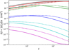Fig. 1. Brightness temperature perturbation power spectrum at z = 0.13 (solid lines) and z = 0.45 (dashed lines) with a 9.33 MHz bandwidth. The auto-spectra of the full signal (black) and of each individual term are shown, generically grouped as Newtonian-gauge density (red), redshift-space distortions (green), velocity term (blue), all potential terms evaluated at the source position (cyan), and the ISW component (magenta). The power spectrum is dominated by the H I overdensity at small scales and has a significant contribution from RSD at large scales.

3. The Fisher matrix

We forecast the constraints from the upcoming 21 cm IM BINGO telescope using the Fisher matrix formalism. The Fisher matrix for the parameters θ_i of a model ℳ is defined as the ensemble average of the Hessian matrix of the log-likelihood. Assuming Gaussian probability distribution with zero mean and covariance C, the Fisher matrix can be calculated as (Tegmark et al. 1997)

$$\begin{array}{c}\hfill F_{\mathit{ij}}\equiv \langle -\frac{\partial ln\mathcal{L}}{\partial {\theta }_i\partial {\theta }_j}\rangle =\frac{1}{2}\mathrm{Tr}\left[{\mathbf{C}}^{-1}\frac{\partial \mathbf{C}}{\partial {\theta }_i}{\mathbf{C}}^{-1}\frac{\partial \mathbf{C}}{\partial {\theta }_j}\right]·\end{array}$$(8)

The covariance C is the sum of the signal and noise spectra estimators. Considering only the thermal and shot noises, it can be written as

$$\begin{array}{c}\hfill \mathbf{C}=C_{\ell }(z_i,z_j)+C_{\ell }^{\mathrm{shot}}(z_i,z_j)+N_{\ell }(z_i,z_j).\end{array}$$(9)

The inverse of the Fisher matrix gives the covariance among the parameters with diagonal elements corresponding to the 1σ marginalized constraints.

Analogously to what is done in the CMB case, we use the a_lm values for the pixelization scheme, where

$$\begin{array}{c}\hfill \langle a_{\ell m}(z_i)a_{{\ell }^{\prime }{m}^{\prime }}^{\ast }(z_j)\rangle ={\delta }_{\ell {\ell }^{\prime }}{\delta }_{m{m}^{\prime }}{C}_{\ell }(z_i,z_j).\end{array}$$(10)

We note that for the CMB all the a_ℓm values are evaluated at the same redshift, while the 21 cm signal has information about a 3D volume that can be analyzed in a tomographic way. Therefore, to extend the covariance matrix to the case of a 21 cm experiment, we use our pixelization as a_ℓm(z). Then, the CMB diagonal matrix is transformed into a diagonal block matrix as

$$\begin{array}{cc}\hfill \mathbf{C}& =\left[\begin{array}{cccc}{A}_{\ell =2}& 0& \dots & 0\\ 0& A_3& \dots & 0\\ ⋮& ⋮& \dots & ⋮\\ 0& 0& \dots & A_n\end{array}\right],\hfill \end{array}$$(11)

where

$$\begin{array}{cc}\hfill A_{\ell }& =(2\ell +1)\left[\begin{array}{cccc}{C}_{\ell }(z_1,z_1)& C_{\ell }(z_1,z_2)& \dots & C_{\ell }(z_1,z_n)\\ C_{\ell }(z_2,z_1)& C_{\ell }(z_2,z_2)& \dots & C_{\ell }(z_2,z_n)\\ ⋮& ⋮& \dots & ⋮\\ C_{\ell }(z_n,z_1)& C_{\ell }(z_n,z_2)& \dots & C_{\ell }(z_n,z_n)\end{array}\right].\hfill \end{array}$$(12)

3.1. Model and parameters

The ΛCDM model is the present cosmological paradigm; it is the simplest model in exquisite agreement with a wide range of cosmological data. In this model the Universe is composed of baryons, photons, neutrinos, DM, and DE, and the gravitational interaction among them is described by general relativity (GR). The Universe begins with an extremely dense and hot plasma. During an early exponential expansion phase, quantum fluctuations in the field driving inflation seeded inhomogeneities in the primordial plasma, providing the initial conditions to all the cosmological structures we observe today. CDM yields the necessary gravitational potentials to amplify the initial fluctuations and DE, assumed as a cosmological constant (Λ), is responsible for the late-time cosmic acceleration. These two components are responsible for about 95% of the energy density budget today.

In this model we assume that the Universe is spatially flat and is governed by six cosmological parameters: Ω_b and Ω_c, the baryon and DM density parameters, respectively, with Ω_i = ρ_i/ρ_c, where ρ_c is the critical density today; h, the Hubble constant parameter H₀ = 100 h km s⁻¹ Mpc⁻¹; the reionization optical depth, τ; the amplitude and spectral index of primordial scalar density perturbations, A_s and n_s, respectively.

The standard model assumes a DE given by a cosmological constant with EoS, w = P/ρ = −1. The simplest extension to this model consists in a dynamical DE with an EoS different from −1. In most of this paper, we use the Chevallier–Polarski–Linder (CPL) parameterization (Chevallier & Polarski 2001; Linder 2003) as our fiducial cosmological model, which allows us to study the constraints on the evolution of the DE EoS. The CPL parameterization is a z-dependent Ansatz for the EoS of DE given by

$$\begin{array}{c}\hfill w_{\mathrm{CPL}}(z)=w_0+w_{\mathrm{a}}\frac{z}{1+z}\mathrm{or}{w}_{\mathrm{CPL}}(a)=w_0+w_{\mathrm{a}}(1-a),\end{array}$$(13)

where w₀ and w_a are constants and ΛCDM is recovered when w₀ = −1 and w_a = 0. Therefore, we vary the Fisher matrix with respect to the following set of cosmological parameters:

$$\begin{array}{c}\hfill \mathit{\theta }=\{{\mathrm{\Omega }}_{\mathrm{b}}{h}^2,{\mathrm{\Omega }}_{\mathrm{c}}{h}^2,h,ln({10}^{10}{A}_{\mathrm{s}}),n_{\mathrm{s}},w_0,w_{\mathrm{a}},b_{\mathrm{H}i}\}.\end{array}$$(14)

In addition, the 21 cm spectra also depends on the H I density parameter Ω_H I, which we fix to its fiducial value. Our ability to constrain this parameter with BINGO and its effect on the cosmological constraints is left to Sect. 4.4.

As our fiducial values we have chosen the best fit from Planck 2018 (Planck Collaboration VI 2020), which we present in Table 1. We have calculated the partial derivatives numerically with a step size of ±0.5%×θ_i. The step size should not be too large, to avoid a miscalculated derivative, nor too small, introducing numerical noise. We checked for the stability of our derivatives to this choice.

BINGO will help put constraints on the late-time Universe parameters. The combination with other probes can break degeneracies among several parameters and improve these constraints. In particular, Planck has provided precise CMB measurements, which gives tight constraints on the standard ΛCDM model. Therefore, we will combine our 21 cm IM forecasts with a prior obtained from the Planck 2018 TT + TE + EE + lowE likelihood data (Planck Collaboration VI 2020). Using the publicly available code CosmoMC (Lewis & Bridle 2002)⁹, we use the Markov chain Monte Carlo (MCMC) technique to estimate the covariance for the cosmological parameters from the Planck data. We then combine the Planck covariance with our 21 cm IM Fisher matrices. It should be noted that, in general, the maximum likelihood from Planck will not coincide with our fiducial values. Here we assume that these constraints do not change significantly over the parameter space.

3.2. Thermal noise

The thermal noise describes the fundamental sensitivity of a radio telescope. It corresponds to the voltages generated by thermal agitations in the resistive components of the antenna receiver. It appears as a uniform Gaussian distribution over the sky, with theoretical noise level per pixel calculated by the radiometer equation (Wilson et al. 2013)

$$\begin{array}{c}\hfill {\sigma }_{\mathrm{T}}=\frac{T_{\mathrm{sys}}}{\sqrt{\mathrm{\Delta }\nu t_{\mathrm{pix}}}},\end{array}$$(15)

where T_sys is the total system temperature (antenna plus sky temperatures), Δν is the frequency channel width, and t_pix is the integration time per pixel, which is related to the total observational time t_obs by

$$\begin{array}{c}\hfill t_{\mathrm{pix}}=t_{\mathrm{obs}}{n}_{\mathrm{beam}}{n}_{\mathrm{f}}\frac{{\mathrm{\Omega }}_{\mathrm{pix}}}{{\mathrm{\Omega }}_{\mathrm{sur}}},\end{array}$$(16)

where n_f denotes the number of feed horns, n_beam is the number of beams and polarizations in each horn, and Ω_pix and Ω_sur describe the pixel and total survey area, respectively.

Assuming the thermal noise between different frequencies are uncorrelated, the noise covariance can be calculated as

$$\begin{array}{c}\hfill N_{\ell }={\sigma }_{\mathrm{T}}^2{\mathrm{\Omega }}_{\mathrm{pix}}=\frac{T_{\mathrm{sys}}^2}{\mathrm{\Delta }\nu t_{\mathrm{obs}}}\frac{{\mathrm{\Omega }}_{\mathrm{sur}}}{2n_{\mathrm{f}}}=\frac{T_{\mathrm{sys}}^2}{\mathrm{\Delta }\nu t_{\mathrm{obs}}}\left(\frac{4\pi f_{\mathrm{sky}}}{2n_{\mathrm{f}}}\right),\end{array}$$(17)

where f_sky is the surveyed fraction of the sky and we have assumed two polarizations are measured.

The telescope also has a maximum beam resolution that should be taken into account. This effect reduces the signal by a factor of $b_{\mathcal{l}}^2$, which is given by (Bull et al. 2015)

$$\begin{array}{c}\hfill b_{\ell }(z_i)=exp(-\frac{1}{2}{\ell }^2{\sigma }_{\mathrm{b},i}^2),\end{array}$$(18)

where ${\sigma }_{\mathrm{b},i}={\theta }_B(z_i)/\sqrt{8ln2}$ with

$$\begin{array}{c}\hfill {\theta }_B(z_i)={\theta }_{\mathit{FWHM}}({\nu }_{\mathrm{center}})\frac{{\nu }_{\mathrm{center}}}{{\nu }_i},\end{array}$$(19)

where ν_center is the middle frequency of the survey. Instead of reducing the signal power spectrum, we can think of the beam resolution as an increase in the noise by the inverse of $b_{\mathcal{l}}^2$.

3.3. Shot noise

Due to the discrete nature of the sources emitting an H I signal, the measured auto-spectra have a shot noise contribution in addition to the clustering part described in Sect. 2. The shot noise power spectrum can be calculated as (Hall et al. 2013)

$$\begin{array}{c}\hfill C_{\ell }^{\mathrm{shot}}=\frac{{\overline{T}}^2(z)}{\overline{N}(z)},\end{array}$$(20)

where $\overline{N}(z)$ is the angular density of the sources; assuming a comoving number density $n=\frac{\mathrm{d}N}{\mathrm{d}V}=0.03h^3$ Mpc⁻³ (Masui et al. 2010), the angular density is given by

$$\begin{array}{c}\hfill \overline{N}(z)=\frac{\mathrm{d}N}{\mathrm{d}\mathrm{\Omega }}=0.03h^3{\mathrm{Mpc}}^{-3}\frac{c}{H_0}{\displaystyle \int }{\chi }^2(z)\frac{\mathrm{d}z}{E(z)}·\end{array}$$(21)

Figure 2 presents these contributions with respect to the H I signal at the first and last redshift bins of BINGO.

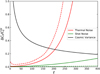Fig. 2. Fractional uncertainties expected for the angular power spectrum for the BINGO experiment (fsky = 0.07) for redshifts z = 0.127 (solid lines) and z = 0.449 (dashed lines) after 1 year of sky integration. The ratio is plotted between different sources of uncertainty (cosmic variance, shot noise, and thermal noise) and the H I angular power spectrum, $\mathrm{\Delta }{C}_{\ell }/C_{\ell }^{\mathrm{H}\mathrm{I}}$, as a function of multipole. For the cosmic variance the standard formula, $\sqrt{2/(2\ell +1)f_{\mathrm{sky}}}$, is used, and for the thermal and shot noise ΔCℓ is equal to their angular power spectrum multiplied by the cosmic variance factor.

3.4. 1/f noise

In addition to the thermal noise, significant contamination will come from the receiver system caused by gain fluctuations, the detector’s temperature changes, quantum fluctuations, and power voltage variations. The power spectrum of this noise is expected to behave as a power law of the frequency. It is generally called pink noise, or more specifically 1/f noise at low frequencies. It introduces stripes along the scan direction in the observed maps (Bigot-Sazy et al. 2015), contaminates the H I signal, and can dominate the Gaussian thermal noise. Therefore, 1/f noise is an important effect that must be taken into account in order to properly detect the H I signal from single-dish IM radio telescopes.

The power spectral density (PSD) combining both the thermal and 1/f noise is the quadratic addition of the two components, given by (Seiffert et al. 2002; Bigot-Sazy et al. 2015)

$$\begin{array}{c}\hfill \mathrm{PSD}(f)={\sigma }_{\mathrm{T}}^2[1+{\left(\frac{f_{\mathrm{knee}}}{f}\right)}^{\alpha }],\end{array}$$(22)

where σ_T is the thermal noise level in Eq. (15), f_knee is the frequency where the 1/f noise has the same amplitude as the thermal noise, and the spectral index α ≈ 1−2 is a parameter. In order to take into account correlations in the frequency direction, an extension to this equation has been proposed by Harper et al. (2018)

$$\begin{array}{c}\hfill \mathrm{PSD}(f,\omega )={\sigma }_{\mathrm{T}}^2[1+{\left(\frac{f_{\mathrm{knee}}}{f}\right)}^{\alpha }{\left(\frac{{\omega }_0}{\omega }\right)}^{\frac{1-\beta }{\beta }}],\end{array}$$(23)

where ω = 1/ν is another parameter, ranging from ω₀ = (NΔν)⁻¹ to ω_N − 1 = (Δν)⁻¹; N is the number of frequency channels with width Δν; and β is the correlation index that describes the 1/f noise correlation in frequency with values in the interval [0,  1]. The 1/f noise will be completely correlated across all frequency channels for β = 0 and completely uncorrelated if β = 1.

The effect of 1/f noise on 21 cm angular power spectra and the final cosmological parameters were analyzed in Chen et al. (2020) for SKA1-MID band 1 and band 2. Here we extrapolate these results for the case of BINGO. Given the redshift range of BINGO, we expect a degradation from 1/f noise that is more similar to what was obtained for SKA1-MID band 2.

In Chen et al. (2020) three cases were considered: with effectively no 1/f noise (completely removed by component separation techniques, β = 0); partially correlated 1/f noise (β = 0.5); and totally uncorrelated 1/f noise (β = 1). The other 1/f noise parameters were kept fixed: the slew speed v_t = 1 deg s⁻¹; the knee frequency f_knee = 1 Hz; and the spectral index α = 1. From the area of the w₀ × w_a joint contour, they found that SKA1-MID band 2 alone was degraded by ≈1.5 with β = 0.5 and ≈2 with β = 1. Combining SKA band 2 with Planck the degradation was less than a factor of ≈1.3 even at β = 1.

As discussed in Chen et al. (2020), higher redshifts and smaller scales are more affected by 1/f noise. BINGO will reach lower redshifts than SKA1-MID band 2 and have a better angular resolution, which amplifies the 1/f noise as in our thermal noise in Sect. 3.2. Therefore, we expect that the 1/f noise will have a degradation factor at most of the same order as found for SKA1-MID band 2 in that paper. Moreover, we aim to obtain with BINGO a knee frequency of ∼1 mHz (Wuensche et al. 2022), which would greatly improve our ability to extract the H I signal. In this paper we do not consider further the effect of 1/f noise.

3.5. Foreground residuals

The success of a 21 cm IM experiment will require the effective removal of galactic and extra-galactic foregrounds that can be up to ∼10⁴ times stronger than the H I signal. This requires refined component separation methods able to properly reconstruct the H I signal immersed in the foreground contamination (Olivari et al. 2016). The foreground cleaning process we plan to apply to the BINGO data are presented in the companion papers (Liccardo et al. 2022; Fornazier et al. 2022). In this paper, we assume the foreground cleaning process has already been performed as part of the BINGO pipeline. However, the foreground cleaning procedure leaves some residuals which are also sources of uncertainties. The component separation method GNILC (Remazeilles et al. 2011a,b; Olivari et al. 2016) projects the observed data into a subspace dominated by H I plus noise and performs an ILC analysis restricted to that space. Therefore, by construction, the foreground residuals should be subdominant. On the other hand, these residuals can introduce a bias in the determination of the 21 cm power spectra and, hence, affect our final cosmological constraints.

We can add this bias to our Fisher matrix formalism following the procedure in Amara & Refregier (2008). For small residual systematics, the bias in the parameter estimation is

$$\begin{array}{c}\hfill b[{\theta }_i]=⟨{\theta }_i⟩-⟨{\theta }_i^{\mathrm{true}}⟩={\displaystyle \sum _j{(F^{-1})}_{\mathit{ij}}{B}_j,}\end{array}$$(24)

where ${\theta }_i^{\text{true}}$ is the true value of the parameters and the bias vector B_j is given by

$$\begin{array}{c}\hfill B_j=\mathrm{Tr}\left[{\mathbf{C}}^{-1}{C}_{\ell }^{\mathrm{sys}}{\mathbf{C}}^{-1}\frac{\partial \mathbf{C}}{\partial {\theta }_j}\right],\end{array}$$(25)

which is similar to the Fisher matrix. In this case the total error covariance matrix is

$$\begin{array}{cc}\hfill \mathrm{Cov}[{\theta }_i,{\theta }_j]& =⟨({\theta }_i-{\theta }_i^{\mathrm{true}})({\theta }_j-{\theta }_j^{\mathrm{true}})⟩\hfill \\ \hfill & ={(F^{-1})}_{\mathit{ij}}+b[{\theta }_i]b[{\theta }_j],\hfill \end{array}$$(26)

including both statistical and systematical errors. Therefore, the presence of foreground residuals should not only increase the parameter uncertainties, but also shift the center of the error ellipses away from the fiducial model.

4. Results

In this section we discuss the expected constraints from the BINGO survey. We adopt the Fisher matrix formalism described in Sect. 3 with the 21 cm angular power spectra presented in Sect. 2. Unless stated otherwise, we consider an optimal scenario where 1/f noise and foreground contamination were already removed using a component separation method (see Liccardo et al. 2022; Fornazier et al. 2022). Therefore, in most of the analysis below we consider the cosmic variance, thermal noise and shot noise only.

First, we discuss the constraints in the basic ΛCDM and in a simple extension, the wCDM model. Then, under the scope of the CPL parameterization, we test the effect of several experimental setups on the final cosmological parameters. We consider the effect of varying the number of feed horns, the total observational time, the number of redshift bins, considering or not cross-correlations between redshift bins, and the effect of RSD. In Sect. 4.3.6 we add foreground residuals in our analysis. Finally, in Sect. 4.3.7 we compare the expected results with SKA band 1 and SKA band 2. Our fiducial experimental setup is given in Table 2 and a more detailed description of the instrument can be found in the companion Paper II (Wuensche et al. 2022).

BINGO will shed light on the H I distribution and evolution at low redshift. In Sect. 4.4 we study the expected constraints on the H I density and bias. We also analyze how BINGO can help constraining the total neutrino mass in Sect. 4.5 and alternative cosmologies in Sect. 4.6.

4.1. The ΛCDM model

The ΛCDM model has been well constrained by the latest CMB measurements made by the Planck satellite, with precision of percent to the sub-percent level on the cosmological parameters (Planck Collaboration VI 2020). In this section we investigate how BINGO can help constrain these parameters.

We performed the Fisher matrix analysis described in Sect. 3 for BINGO and for BINGO and Planck combined (BINGO + Planck). The results are presented in Table 3. In the second column of Table 3 we note that BINGO alone cannot put competitive constraints on the cosmological parameters from Table 1. However, the combination of the two surveys can improve the confidence in all cosmological parameters (Col. 4 of Table 3). The most significant improvements are in the DM density parameter, Ω_ch², and the Hubble parameter, h, by more than 25% in both of them. This is on the same order as what has been currently obtained by adding CMB lensing and BAO to the final Planck temperature and polarization results (cf. Table 2 in Planck Collaboration VI 2020). We can also see that the primordial density parameters, A_s and n_s, are mostly constrained by Planck itself with an enhancement of 3.8% and 8.7%, respectively. The uncertainty on the baryon fraction, parameterized by Ω_bh², decreases by 11%.

On the other hand, the most important contribution from 21 cm experiments will not be reducing these error bars, but providing additional information from a different tracer of the matter distribution. Although the ΛCDM model has been in good agreement with data, recent observations have pointed out severe tensions between the CMB and low redshift data under the ΛCDM scenario. Riess et al. (2019) obtained a 4.4σ deviation of the value for the Hubble constant measured by Planck and the one using Cepheids in the Large Magellanic Cloud. Measurements from weak gravitational lensing have also pointed out a disagreement of 2.3σ for the value of $S_8={\sigma }_8\sqrt{{\mathrm{\Omega }}_{\mathrm{m}}/0.3}$ obtained with Planck data (Hildebrandt et al. 2020). Therefore, a new and independent tracer of the matter distribution, with different systematics, will provide valuable information and improve our understanding of the evolution of the Universe. Our projected constraints show that BINGO alone will not have enough power to solve these tensions; however, it can be combined with other constraints and will also open the way to more precise 21 cm experiments in the future.

4.2. wCDM model

Because of the extra freedom in the parameter space, the previous constraint from Planck data in the Hubble constant is loosened. The 1% precision measurement for the Hubble constant at 1σ in the ΛCDM model goes to ∼13% in the wCDM model. The ability to constrain the DE EoS using CMB information only is also rather weak, providing 25% uncertainty at a 1σ confidence level (CL). In this case additional data at low redshifts where DE dominates is crucial.

The 21 cm IM power spectra measured by BINGO will be able to improve these constraints. In Table 4 we show the expected constraints in the wCDM model by BINGO and in combination with Planck. We can see that BINGO alone will be able to put similar constraints to those from Planck on the Hubble constant and a 17% precision measurement at 1σ CL on the DE EoS. Combining them can greatly improve these results, reaching a remarkable precision of 1.1% for H₀ and 3.3% for the EoS, which are consistent with previous results obtained by Olivari et al. (2018). The reason for this improvement can be observed in Fig. 3. BINGO can help break the degeneracy between H₀ and w in the Planck data, dramatically improving the constraints.

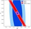Fig. 3. Marginalized constraints (68% and 95% CL) on the DE EoS and Hubble parameters for the wCDM model using BINGO, Planck, and BINGO + Planck.

As a comparison, recent measurements from the three years of the Dark Energy Survey (DES) (Abbott et al. 2021) using three two-point correlation functions (from cosmic shear, galaxy clustering, and cross-correlation of source galaxy shear with lens galaxy positions) over 5000 deg² obtained a constraint on the DE EoS of $\mathit{w}=-0.{98}_{-0.20}^{+0.32}$. Combining their measurement with Planck (no lensing), their marginalized constraint is given by $\mathit{w}=-1.{090}_{-0.113}^{+0.128}$. Therefore, although we are still performing an optimistic analysis, we can see that BINGO has the potential to put constraints that is competitive with the current LSS surveys.

4.3. CPL parameterization

Considering the BINGO fiducial setup, we show the forecast constraints on the CPL parameterization in Table 5. The additional parameter increased the uncertainties on the cosmological variables, as expected. The combination of 21 cm IM from BINGO with CMB data from Planck can put a 2.9% constraint on the Hubble constant, 30% on the DE EoS parameter w₀, and a σ_wa = 1.2 at 68% CL. Although these constraints are still large, BINGO has improved the results from Planck alone by 78% for H₀, 34% for w₀, and 31% for w_a. Figure 4 shows the 68% and 95% confidence contours in the w₀ × w_a parameter space.

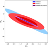Fig. 4. Marginalized constraints (68% and 95% CL) on the DE EoS parameters for the CPL parameterization using BINGO, Planck, and BINGO + Planck.

Yohana et al. (2019) have made a forecast for BINGO using the angular power spectra under the CPL parameterization. Their analysis considers the same cosmological parameters used here plus the effective number of relativistic neutrinos, N_eff, and the sum of neutrino masses, ∑m_ν. The H I bias was kept fixed. Their projected constraints for the DE EoS parameters were significantly weaker than ours, while for the Hubble constant it was more than two times stronger. Although the degradation in the DE EoS parameters can be understood in terms of the extra degrees of freedom, the difference in the Hubble constant may be related to differences in the analysis and BINGO setup.

4.3.1. Effect of total observational time

Using the CPL parameterization as our fiducial cosmology, we analyze how different experimental setups can impact our final measurements of cosmological parameters. We start by considering the impact of BINGO’s total observational time. Figure 5 presents the results for 1, 2, 3, 4, and 5 years of the BINGO survey. We show the results for BINGO only and in combination with Planck. Considering BINGO alone, a five-year experiment can improve the constraints in a range from 21% to 35%. We can observe that the inclination of these curves decreases, going to a plateau, but it has not yet been achieved at five years.

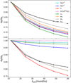Fig. 5. Constraints on the cosmological and H I parameters as a function of the total observational time relative to those with tobs = 1 year for BINGO (top) and BINGO + Planck (bottom). We vary tobs in a range of [1,  2,  3,  4,  5] years. In the bottom plot wa is on top of w0, which cannot be seen.

In order to better evaluate the improvement in our parameter space, we calculate the figure of merit (FoM), defined as the volume of the error ellipsoid FoM ≡ V ∝ det(F)^−1/2. Table 6 presents these values for BINGO and BINGO + Planck as a function of the total observational time. We can observe that the ellipsoid volume decreases by 11 times from 1 year to 5 years with BINGO only, and significantly flattens after year 3.

On the other hand, the combination with Planck data shows that some parameters are not strongly dependent on the BINGO setup since they are mostly constrained by Planck. BINGO will mainly affect the measurement of the Hubble constant, DE EoS parameters, and the H I bias, as has already been observed (Olivari et al. 2018). A five-year experiment can improve the bias measurement by 19%, the EoS parameters (w₀ and w_a) by about 21% each, and the Hubble constant by 25% compared to the standard case. Combining the two surveys, the error ellipsoid decreases by 2.7 times from 1 to 5 years of IM survey.

4.3.2. Effect of varying the number of horns

In this section we consider the effect of the total number of feed horns. As described in Table 2, the BINGO standard setup will consist of 28 feed horns. In Fig. 6 we represent the BINGO + Planck standard scenario by a star. Then, keeping all parameters fixed and only varying the number of horns as N_horns = 20, 30, 40, 50, 60, we observe its effect on the cosmological constraints. We observe that some parameters are mainly constrained by Planck and, therefore, will not be very sensitive to BINGO’s number of horns. The most affected parameters are the DE EoS parameters, the Hubble constant, and the H I bias. They improve by about 15% with respect to N_horns = 20, more specifically δw₀ and δw_a = 14%, δb_H I = 16%, and δh = 17%.

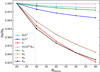Fig. 6. Constraints on the cosmological and H I parameters as a function of the number of feed horns for BINGO + Planck.

We observe, however, that these curves are only taking into account how the number of horns affects the thermal noise without changing the total observational area. A simple telescope design with drift scan only may not be able to cover the same fraction of the sky if the number of horns is too small. Several horn arrangements are discussed in the BINGO companion paper (Abdalla et al. 2022b): a rectangular configuration (n_f = 33), a double-rectangular configuration (n_f = 28), and a hexagonal configuration (n_f = 49). In all cases the total surveyed area was kept constant. In this case, as can be observed in Eq. (17), varying the total observational time or the number of horns produces the same result if they change accordingly.

4.3.3. Effect of the number of redshift bins

Our analysis of the volume surveyed by BINGO was done using the 21 cm angular power spectra in redshift bins. The angular power spectrum projects all contributions inside a thin shell. Therefore, we can make a tomographic analysis of the Universe volume. If we sliced that volume into thinner shells, we could obtain a more detailed observation; however, as can be observed in Eq. (17), thinner shells also mean larger thermal noise. Therefore, we expect an optimal number of slices beyond which no more cosmological information could be extracted from a specific survey. In addition, the number of necessary calculations to take all auto- and cross-correlated C_ℓs into account increases as we increase the number of redshift bins, hence it is desirable to keep this number as small as possible for computational purposes.

We study this behavior with the BINGO telescope considering N_bin = 2, 4, 8, 16, 32, 64, 128, which implies in equally spaced frequency bins with bandwidths equal to Δν = 140, 70, 35, 17.5, 8.75, 4.375, 2.187 MHz. Figure 7 presents our results for BINGO and for BINGO + Planck. We can see that increasing the number of bins can greatly improve several cosmological constraints, especially those related to the late-time cosmic acceleration. On the other hand, there is not much difference from N_bin = 64 to N_bin = 128 and a plateau has been reached for several parameter uncertainties. The projected uncertainties with BINGO for N_bin = 128 relative to N_bin = 2 have improved by about 92 times for w_a, 74 times for w₀, 55 times for b_H I, 18 times for ln(10¹⁰A_s) and h, 17 times for Ω_bh², 15 times for Ω_ch², and 12 times for n_s. On the other hand, if we compare our results for N_bin = 128 with N_bin = 64, the maximum improvement is of 1.8 times for w_a. The comparison with N_bin = 32, which is close to our fiducial value, shows that N_bin = 128 improves our constraints by about 4 times for the DE EoS parameters w₀ and w_a, 3 times for b_H I, and 2 times for the other parameters. In the case of BINGO + Planck, the constraints with N_bin = 128 are smaller than those with N_bin = 2 by about 11 times for b_H I, 5 times for h, 3 times for w₀ and w_a, 1.7 times for Ω_ch², 1.2 times for Ω_bh² and n_s, and is negligible for ln(10¹⁰A_s). Comparing N_bin = 128 with N_bin = 64, the largest improvements are 1.5 times for the DE EoS parameters, followed by the Hubble constant with an uncertainty that is 1.4 times smaller.

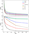Fig. 7. Projected constraints on the cosmological and H I parameters as a function of the number of bins for BINGO (top) and BINGO + Planck (bottom). They show that w0, wa, and h can have their constraints further improved for Nbin > 30.

4.3.4. Effect of cross-correlations

Previous analyses in the literature considered the Limber approximation to forecast 21 cm IM constraints (Olivari et al. 2018). The Limber approximation does not take into account the cross-correlations between redshift bins, only the auto-correlation spectra. Although this allows a faster and simpler calculation, we miss part of the information contained in the whole spectra. Here we study the effect including all information using the full power spectra. We demonstrate that effect in Fig. 8, where we calculate the percentage difference between the results with and without cross-correlation (Δσ_θ/σ_θ = σ_θ without/σ_θ with − 1) as a function of the number of bins. As can be seen, the importance of cross-correlations increases as we increase the number of bins, but it eventually reaches a plateau. For N_bin = 32, which is close to the fiducial BINGO setup, we find that the cross-correlations improve the constraints by δln(10¹⁰A_s) = 0.4%, δΩ_bh² = 6.8%, δn_s = 7.2%, δh = 8.3%, δw₀ = 8.8%, δw_a = 11%, δΩ_ch² = 22%, and δb_H I = 31%. The primordial spectrum amplitude, A_s, is the least affected by cross-correlations as it is basically constrained by Planck data. At the maximum number of bins considered, these constraints have improved to δln(10¹⁰A_s) = 1.7%, δΩ_bh² and δn_s = 14%, δh = 25%, δw₀ = 29%, δw_a = 31%, δΩ_ch² = 65%, and δb_H I = 90%.

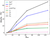Fig. 8. Percentage difference between using and not using information from the cross-correlations in the projected cosmological parameter constraints expected for BINGO + Planck.

4.3.5. Effect of RSD

Another feature that is worth investigating is the effect of RSD. First, we observe that without RSD the primordial scalar amplitude and the H I bias are completely degenerate. RSD is able to break that degeneracy and allows us to constrain these parameters individually with 21 cm data alone. We show the percentage difference between the Fisher matrix results with and without RSD (Δσ_θ/σ_θ = σ_θ without/σ_θ with − 1) in Fig. 9. The parameters A_s and b_H I go from a complete ignorance to constraints on the order of the percent level, and therefore we do not include them in the plot with BINGO alone. Second, we expect RSD to become more and more important as the frequency (or redshift) smoothing width gets narrower. This happens because the angular spectra sum up all contributions inside the bin, and hence a large bandwidth will cancel out the contributions. This behavior can be seen in Fig. 9, where there is a tendency for RSD to improve the cosmological constraints as we decrease the bandwidth.

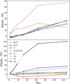Fig. 9. Percentage difference between using and not using information from RSD in the cosmological parameter constraints from BINGO (top) and BINGO + Planck (bottom).

Considering BINGO alone, the most significantly affected parameters by RSD at N_bin = 32 are the EoS parameters, with δw₀ = 13% and δw_a = 30%. The other parameters improve by at most ∼3%. Increasing the number of bins, we achieve a difference between using and not using RSD in a range from ∼15% to ∼57% at N_bin = 128. If we combine our H I results with CMB data from Planck, the CMB measurements can put constraints on the amplitude of the primordial spectrum, A_s, and break the degeneracy with our H I bias even if we do not consider RSD. Figure 9 also includes the results in combination with CMB data. The addition of Planck data will put tight constraints on and will affect the correlation between several parameters; therefore, RSD from our 21 cm IM spectra will behave differently from the earlier results. We can observe this in the behavior of the Hubble constant parameter, which increases the uncertainty with the inclusion of RSD for several values of redshift bins. At N_bin = 128 the improvements from RSD are given by δh = 1%, δln(10¹⁰A_s) = 2.2%, δΩ_bh² = 7.8%, δn_s = 9.5%, δw₀ = 14%, δw_a = 34%, δΩ_ch² = 44%, and δb_H I = 176%.

4.3.6. Effect of foreground residuals

Our results so far have considered a perfect foreground cleaning process. However, as discussed in Sect. 3.5, these procedures leave residuals that can bias the parameter estimation and increase the statistical noise. In order to take these effects into account, we assume that there has already been some sort of foreground removal technique and model the residual contamination as the sum of Gaussian processes with angular power spectra given by (Santos et al. 2005; Bull et al. 2015)

$$\begin{array}{c}\hfill C_{\ell }^{\mathrm{FG}}({\nu }_1,{\nu }_2)={ϵ}_{\mathrm{FG}}^2{\displaystyle \sum _i{A}_i{\left(\frac{{\ell }_{\mathrm{ref}}}{\ell }\right)}^{{\beta }_i}{\left(\frac{{\nu }_{\mathrm{ref}}^2}{{\nu }_1{\nu }_2}\right)}^{{\alpha }_i}exp(-\frac{{log}^2({\nu }_1/{\nu }_2)}{2{\xi }_i^2})·}\end{array}$$(27)

We assume four foreground contributions with the parameters described in Table 7. The overall scaling, ϵ_FG, parameterizes the efficiency of the foreground removal technique, with ϵ_FG = 1 corresponding to no foreground removal.

The additional contribution from foreground residuals increases the covariance given by Eq. (9), and consequently enlarges the statistical errors on the final cosmological parameters. The ratios of the marginalized 1σ constraints with respect to the case without foreground residuals are plotted in Fig. 10 as a function of the residual amplitude ϵ_FG. We find the constraints are degraded by at most 16% in the case of BINGO only, and 6% for BINGO + Planck. If the efficiency of foreground removal is ϵ_FG < 10⁻⁵, these effects are negligible.

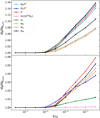Fig. 10. Marginalized statistical errors as a function of the residual foreground contamination amplitude, ϵFG, from BINGO (top) and BINGO + Planck (bottom).

The residuals will also shift the cosmological parameters from their true value according to Eq. (24), with $C_{\mathcal{l}}^{\text{sys}}=C_{\mathcal{l}}^{\text{FG}}$. Figure 11 shows the ratio of bias to the marginalized statistical errors as a function of ϵ_FG. We find that unlike the marginalized constraints that always decrease as ϵ_FG goes to zero, the bias presents an unpredictable behavior for large values of the residual amplitude. This can be understood from Eq. (25), which basically depends on the foreground residuals as $\frac{C_{\ell }^{\mathrm{FG}}}{{(C_{\ell }+C_{\ell }^{\mathrm{shot}}+N_{\ell }+C_{\ell }^{\mathrm{FG}})}^2}$. This function increases as we decrease $C_{\mathcal{l}}^{\text{FG}}$, and has a maximum at $C_{\mathcal{l}}^{\text{FG}}=C_{\mathcal{l}}+C_{\mathcal{l}}^{\text{shot}}+N_{\mathcal{l}}$. The bias procedure in Eq. (24) is valid when $C_{\mathcal{l}}^{\text{sys}}$ is small compared to C, which in our case happens for ϵ_FG ≲ 10⁻⁴. Considering a foreground removal process with ϵ_FG = 10⁻⁴, the largest bias was |b[Ω_ch²]| = 0.9σ and |b[Ω_ch²]| = 1σ for BINGO and BINGO + Planck, respectively. Figure 12 shows the marginalized constraints for the DE EoS parameters considering both statistical and systematic errors with BINGO.

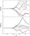Fig. 11. Ratio of bias to the marginalized statistical errors for each parameter as a function of the residual foreground contamination amplitude, ϵFG, from BINGO (top) and BINGO + Planck (bottom).

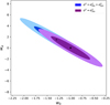Fig. 12. Marginalized constraints (68% and 95% CL) on the DE EoS parameters for the CPL parameterization with BINGO, considering the effect of foreground residuals on the statistical and systematic errors. The star corresponds to our fiducial value and the cross shows the value recovered given the Fisher matrix bias. We have fixed ϵFG = 10−4.

4.3.7. Comparison with SKA

We now compare the expected constraints from BINGO with the experiment design for SKA1-MID band 1 and SKA1-MID band 2 (Bacon et al. 2020). We consider the same experimental setup for SKA as used in Chen et al. (2020), except that we use a bandwidth of 10 MHz. In order to have a proper comparison between them, in this section we only use 28 redshift bins for BINGO, which implies a bandwidth of 10 MHz, consistent with the value used for the SKA results. This produces a small degradation in our forecast in comparison with the fiducial scenario presented in Table 5. We compare the marginalized constraints on our eight-parameter space in Fig. 13 and Table 8. For a better comparison, we also repeat the constraints from Planck alone from Table 5.

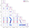Fig. 13. One- and two-dimensional (68% and 95% CL) cosmological constraints for a CPL parameterization from BINGO, SKA1-MID band 1, and SKA1-MID band 2 in combination with Planck data. This illustrates that BINGO can be considered a pathfinder for constraints obtained by SKA.

Even considering the power of SKA, we can observe that several cosmological parameters are mainly constrained by Planck, although small improvements are still possible, especially breaking degeneracies in the parameter space. Their main contributions are in the DE EoS parameters and the Hubble constant. The Hubble constant improved from a projected constraint of 13% with Planck alone to 2.9%, 1%, and 0.5% in combination with BINGO, SKA Band 1, and SKA Band 2, respectively. In addition, the DE EoS parameter w₀ goes from 46% to 31%, 8%, and 3.2%. Finally, we obtained a projected constraint for w_a of 1.8, 1.2, 0.26, and 0.037 from Planck, BINGO + Planck, SKA Band 1 + Planck, and SKA Band 2 + Planck, respectively. For all these parameters, SKA Band 2 showed the best constraints. Generally, these results are in agreement with what was found in Chen et al. (2020) for the SKA. Some discrepancies may be related to our larger number of bins and the fact that we are considering dimensional C_ℓs. This better takes into account the dependence with the brightness temperature in the Fisher matrix derivatives.

Both SKA band 1 and band 2 will survey a larger fraction of the sky than BINGO. They are also designed to explore a wider redshift range. In addition, although BINGO has a better angular resolution, the number of antennas is much lower than for SKA and the system temperature is higher. Combining all these aspects favors SKA in the ability to constrain cosmology. On the other hand, SKA will require a more complicated technique combining the dish array for a IM single-dish mode. Therefore, the simplicity of the BINGO instrument will be a pathfinder for IM with SKA. In particular, Table 8 shows BINGO can provide valuable information for the H I bias.

4.4. HI,density and bias

Using the 21 cm line of H I as a tracer of the underlying matter distribution requires the knowledge of the H I mean density and bias. If we are only interested in the cosmological constraints, they can be considered nuisance parameters that we marginalize over. On the other hand, we can also use our 21 cm survey to learn about their distribution and evolution.

In the previous sections we fix the value for the H I density parameter, Ω_H I, and described the bias by a constant in the whole redshift range. We now extend these assumptions and see their impact in our cosmological parameters and our ability to constrain them with BINGO.

First we fix the H I density parameter and assume a constant bias. Table 3 shows that we can achieve a 4.1% precision measurement in the bias with BINGO under the ΛCDM model, which can be improved to 1.1% if we combine with Planck data. Beyond the ΛCDM model, the constraints are degraded by the extra cosmological parameters, but we still obtain a 2.3% precision measurement at 1σ in the joint analysis BINGO + Planck, as calculated in Tables 4 and 5.

Next, we extend this simplest model and allow Ω_H I to be a free parameter. Equations (1), (6), and (7) tell us that in this case Ω_H I and A_s are completely degenerate, and therefore we cannot constrain them with BINGO alone. In order to break that degeneracy, we combine our analysis with Planck. Our results are presented in Table 9. We obtain

$$\begin{array}{cc}\hfill {\sigma }_{{\mathrm{\Omega }}_{\mathrm{H}i}}& =4.1\times {10}^{-5}(6.6\%),\hfill \end{array}$$(28)

$$\begin{array}{cc}\hfill {\sigma }_{b_{\mathrm{H}i}}& =3.6\times {10}^{-2}(3.6\%).\hfill \end{array}$$(29)

Compared with the fiducial model presented in Table 5, the parameter most affected by the inclusion of Ω_H I is the bias, with a degradation of 61%. The next most sensitive is the DM density parameter, Ω_ch², which is degraded by 15%, followed by the DE EoS parameter, w_a, which has its uncertainty increased by 9.5%. The other parameters change by at most ∼5%.

A natural extension to this model is to assume that the H I parameters evolve with redshift. We use a stepwise model, which is simple and provides an agnostic way to describe the evolution of these parameters over redshift. Therefore, we combine our 30 redshift bins into three groups and define the parameters as ${\mathrm{\Omega }}_{\mathrm{H}\mathrm{I}}^i$ and $b_{\mathrm{H}\mathrm{I}}^i$ inside each group. We first consider the H I density as a function of redshift, keeping the bias constant. In this case our constraints are given by

$$\begin{array}{cc}\hfill {\sigma }_{{\mathrm{\Omega }}_{\mathrm{H}i}^1}& =4.5\times {10}^{-5}(7.2\%),\hfill \end{array}$$(30)

$$\begin{array}{cc}\hfill {\sigma }_{{\mathrm{\Omega }}_{\mathrm{H}i}^2}& =4.6\times {10}^{-5}(7.4\%),\hfill \end{array}$$(31)

$$\begin{array}{cc}\hfill {\sigma }_{{\mathrm{\Omega }}_{\mathrm{H}i}^3}& =4.8\times {10}^{-5}(7.7\%),\hfill \end{array}$$(32)

$$\begin{array}{cc}\hfill {\sigma }_{b_{\mathrm{H}i}}& =3.7\times {10}^{-2}(3.7\%),\hfill \end{array}$$(33)

where the indices 1, 2, and 3 represent each group of ten redshift bins. The projected constraints are very similar in all three groups of bins, but lower redshifts show slightly better results. In addition, the projected bias is only marginally affected by the extra degrees of freedom in the H I density parameter.

Finally, we consider the case where both Ω_H I and b_H I are functions of redshift. Our results are presented in Table 9 together with the previous scenarios. The extra parameters describing the H I distribution and evolution mainly affect our uncertainties on the cosmological parameters describing the DE EoS (degrading by δw₀ = 4.9% and δw_a = 5.5%) and the Hubble constant (with δh = 2.3%) compared with the previous case. The other CPL parameters are not significantly impacted as Planck is mainly responsible for their constraints. On the other hand, the H I bias constraints vary by at most 88%. This last scenario can put constraints on the H I parameters with uncertainties of around 8.5% and 6% for the H I density parameter and bias, respectively:

$$\begin{array}{cc}\hfill {\sigma }_{{\mathrm{\Omega }}_{\mathrm{H}i}^1}& =5.4\times {10}^{-5}(8.7\%),\hfill \end{array}$$(34)

$$\begin{array}{cc}\hfill {\sigma }_{{\mathrm{\Omega }}_{\mathrm{H}i}^2}& =5.2\times {10}^{-5}(8.4\%),\hfill \end{array}$$(35)

$$\begin{array}{cc}\hfill {\sigma }_{{\mathrm{\Omega }}_{\mathrm{H}i}^3}& =5.6\times {10}^{-5}(9\%),\hfill \end{array}$$(36)

$$\begin{array}{cc}\hfill {\sigma }_{b_{\mathrm{H}i}^1}& =6.9\times {10}^{-2}(6.9\%),\hfill \end{array}$$(37)

$$\begin{array}{cc}\hfill {\sigma }_{b_{\mathrm{H}i}^2}& =5.8\times {10}^{-2}(5.8\%),\hfill \end{array}$$(38)

$$\begin{array}{cc}\hfill {\sigma }_{b_{\mathrm{H}i}^3}& =5.9\times {10}^{-2}(5.9\%).\hfill \end{array}$$(39)

Further details about the H I distribution using N-body simulations can be obtained in our BINGO companion paper (Zhang et al. 2022).

4.5. Massive neutrinos

It is well known that neutrinos should have a low mass in order to explain their change of flavors, observed in both solar and atmospheric neutrinos (Fukuda et al. 1998; Ahmad et al. 2002). However, the experiments only allow us to determine two squared mass differences. On the other hand, it is possible to constrain the sum of neutrino masses, ∑m_ν, from a combination of the CMB and matter power spectrum.

Massive neutrinos can impact the CMB spectrum in different ways. At the background level they may change the redshift of matter-to-radiation equality, the angular diameter distance to the last scattering surface, and the late ISW effect, while neutrino perturbations affect the early ISW effect (Lesgourgues & Pastor 2012). In order to analyze the constraints on the total neutrino mass, we consider an extension to the ΛCDM model allowing for an extra degree of freedom on the sum of neutrino masses, ΛCDM + ∑m_ν. We performed a MCMC sampling with the Planck 2018 TT + TE + EE + lowE likelihood, assuming one massive neutrino with total mass equal to ∑m_ν. Our result is given by

$$\begin{array}{c}\hfill {\sigma }_{\sum m_{\nu }}<0.36\mathrm{eV}(95\%\mathrm{CL},\mathit{Planck}).\end{array}$$(40)

This is higher than the value of 0.26 eV reported in Planck Collaboration VI (2020) using the Plik likelihood, but below the value of 0.38 eV from the CamSpec likelihood. For the purpose of this forecast paper, we use the value we report above.

The combination of CMB data with other cosmological observations, such as measurements of the H I power spectrum, can break the geometric degeneracy in the parameter space of the ΛCDM + ∑m_ν model and improve the constraints. We combined the covariance matrix from the Planck data with our 21 cm Fisher analysis, and this leads to

$$\begin{array}{c}\hfill {\sigma }_{\sum m_{\nu }}<0.14\mathrm{eV}(95\%\mathrm{CL},\mathrm{BINGO}+\mathit{Planck}),\end{array}$$(41)

which is slightly higher than what was obtained in Planck Collaboration VI (2020) for the combination between Planck temperature and polarization with other BAO data. Therefore, if BINGO’s systematic noise can be properly taken into account, it will be able to put competitive constraints on the sum of neutrino masses compared with the present available constraints, but using a completely independent tracer of LSS.

4.6. Alternative cosmologies

4.6.1. Modified Gravity: μ and Σ parameterization

An alternative explanation for the accelerated expansion of the Universe is to invoke modifications of GR. To properly describe the current data, these modifications must explain the current acceleration with background dynamics very close to the ΛCDM predictions today, while maintaining the local and astrophysical tests of GR. There are several proposed modifications of gravity in the literature (for a review see Clifton et al. 2012) with the most studied being scalar-tensor theories and higher-derivative theories, such as f(R). The f(R) theory is the simplest modification of GR and can be mapped onto a scalar-tensor theory via field redefinition and conformal transformation. A more general class of scalar-tensor theories are the Horndeski models (Horndeski 1974), a class of models that modify GR while still maintaining up to second-order derivatives in the equations of motion, avoiding instabilities (Deffayet et al. 2011). Although the background evolution of these modifications of GR needs to behave close to ΛCDM today, the evolution of their perturbations might behave very differently, and that represents an avenue to test these models.

Modified gravity (MG) models can be parameterized through two phenomenological functions, μ and γ. On sub-Hubble scales, the Poisson equation and the relation between the gravitational potentials receive corrections if gravity is modified, given by

$$\begin{array}{cc}\hfill -k^2\mathrm{\Psi }& =4\pi G{a}^2\mu (a,k)\overline{\rho }\mathrm{\Delta },\hfill \\ \hfill \mathrm{\Phi }& =\gamma (a,k)\mathrm{\Psi },\hfill \end{array}$$(42)

where $\overline{\rho }$ is the background value of the matter energy density, Δ = δ + 3ℋv/k is the comoving density perturbation with ℋ the conformal time Hubble parameter, δ is the density contrast, and where the anisotropic stress from relativistic species was neglected. The parameters μ and γ represent deviations from GR, since in GR μ = γ = 1 at all times, while for alternative models both functions can depend upon time and scale. Using these equations, the variation of the energy-momentum tensor of a scalar tensor theory in the Jordan frame yields the continuity and Euler equations on sub-Hubble scales (Hall et al. 2013)

$$\begin{array}{cc}\hfill \ddot{\delta }+\mathcal{H}\dot{\delta }-4\pi G{a}^2\mu \overline{\rho }\delta & =0,\hfill \end{array}$$(43)

$$\begin{array}{cc}\hfill \ddot{v}+(2\mathcal{H}-\frac{\dot{\mu }}{\mu })\dot{v}+(\dot{\mathcal{H}+{\mathcal{H}}^2-\mathcal{H}}\frac{\dot{\mu }}{\mu }-4\pi G{a}^2\mu \overline{\rho })v& =0.\hfill \end{array}$$(44)

These equations show that the density perturbation and velocity depend only on changes in μ on subhorizon scales. Changes in the density and velocities can be probed by experiments like BINGO since the 21 cm brightness temperature is sensitive to density and RSD, offering a chance to probe the time and scale dependence of the parameter μ.

To project constraints on the cosmological parameters, we use the results from BINGO combined with data from the CMB. Modifications of gravity that aim to explain the late-time acceleration only affect the CMB at perturbed level via the ISW effect in the CMB temperature anisotropies and via CMB weak lensing. This is a result of the time dependency of the potentials Φ and Ψ. The CMB is sensitive to modifications of the Weyl potential, given by (Φ + Ψ)/2, which can be related to the density perturbation from Eq. (42),

$$\begin{array}{c}\hfill -k^2(\mathrm{\Phi }+\mathrm{\Psi })=8\pi G{a}^2\mathrm{\Sigma }(a,k)\overline{\rho }\mathrm{\Delta },\end{array}$$(45)

where Σ(a, k)≡μ(1 + γ)/2. Due to the degeneracy between μ and γ, it can be more convenient to work with this new function Σ (Daniel et al. 2010).

In order to forecast constraints on MG models with the BINGO telescope, we consider a specific form for that parameterization that is related to f(R) theories of gravity. The B₀-parameterization of f(R) gravity provides a good approximation on quasi-static scales (Hu & Sawicki 2007; Giannantonio et al. 2010; Hojjati et al. 2012), and has a parameterization given by

$$\begin{array}{cc}\hfill \mu (a,k)& =\frac{1}{1-1.4\times {10}^{-8}{|\lambda /\mathrm{Mpc}|}^2{a}^3}\frac{1+4{\lambda }^2{k}^2{a}^4/3}{1+{\lambda }^2{k}^2{a}^4},\hfill \end{array}$$(46)

$$\begin{array}{cc}\hfill \gamma (a,k)& =\frac{1+2{\lambda }^2{k}^2{a}^4/3}{1+4{\lambda }^2{k}^2{a}^4/3},\hfill \end{array}$$(47)

where $B_0\equiv 2H_0^2{\lambda }^2$. Therefore, considering the ΛCDM parameters plus B₀, we obtained a projected constraint of

$$\begin{array}{cc}\hfill {\sigma }_{B_0}& =3.1\times {10}^{-5}(\mathrm{BINGO}),\hfill \end{array}$$(48)

$$\begin{array}{cc}\hfill {\sigma }_{B_0}& =5.3\times {10}^{-2}(\mathit{Planck}),\hfill \end{array}$$(49)

$$\begin{array}{cc}\hfill {\sigma }_{B_0}& =1.1\times {10}^{-5}(\mathrm{BINGO}+\mathit{Planck}).\hfill \end{array}$$(50)

Figure 14 shows the 2D marginalized contours for B₀ and h. We can see that BINGO will lead to a tight constraint on the MG parameter and also how the combination with Planck breaks the degeneracy in the parameter space. We note that the tight constraint on the Hubble constant from Planck comes from the fact we have assumed the ΛCDM model for the cosmological background.

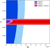Fig. 14. Marginalized constraints (68% and 95%) CL on the modified gravity parameter B0 and the Hubble parameter from BINGO, Planck, and BINGO + Planck.

4.6.2. Interacting dark energy

Another possible modification of the ΛCDM is to consider an interaction in the dark sector (Wetterich 1995; Amendola 2000). Since the dark sector is only detected gravitationally, different types of interaction of DE and DM are possible (Wang et al. 2016). In a field theory description of these components, this interaction is allowed and even mandatory (Micheletti et al. 2009). It can also alleviate the coincidence problem, given an appropriate interaction and a dynamical mechanism to make DE leave the scaling solution and produce late acceleration (Copeland et al. 2006).

The study of the interacting dark sector model is challenging because of the unknown nature of the two components, which makes it hard to describe the origin of such an interaction from first principles. Many different models of this interaction have been studied in the literature either from a phenomenological or from a field theory point of view. Here we take a purely phenomenological approach to describe the interacting dark sector (for a more general description of the classification of these models see Wang et al. 2016; Koyama et al. 2009; Pu et al. 2015; Ferreira et al. 2017; Costa et al. 2014, 2015; Marcondes et al. 2016; Landim & Abdalla 2017; Landim et al. 2018).

The interaction acts so that the energy-momentum of the dark sector components alone does not obey a conservation law,

$$\begin{array}{c}\hfill {\mathrm{\nabla }}_{\mu }{T}_{(i)}^{\mu \nu }=Q_{(i)}^{\nu },\end{array}$$(51)

where conservation of the total energy-momentum implies that the right-hand sides add up to zero, $\sum _i{Q}_{(i)}^{\nu }=0$. This is how the interaction can be realized.

Given the energy conservation of the full energy-momentum tensor, we represent DE and DM as fluids in a Friedmann-Lemaître-Robertson-Walker (FLRW) Universe obeying

$$\begin{array}{cc}& {\dot{\rho }}_{\mathrm{dm}}+3H{\rho }_{\mathrm{dm}}=+Q,\hfill \\ \hfill & {\dot{\rho }}_{\mathrm{de}}+3H(1+w_{\mathrm{de}}){\rho }_{\mathrm{de}}=-Q,\hfill \end{array}$$(52)

where ρ_dm and ρ_de are the energy densities of DM and DE, respectively, and the interaction Q can be a function of ρ_dm, ρ_de, or both. We assume that the EoS is constant in this simple model. By this definition if Q > 0, we have DE decaying in DM and for Q < 0 we have DM decaying in DE. The second case favors a Universe dominated by DM in the past and DE in the future. The interaction Q(ρ_dm, ρ_de) can be expanded in a Taylor series, and the phenomenological term (Feng et al. 2008; He et al. 2011)

$$\begin{array}{c}\hfill Q=3H({\xi }_{\mathrm{dm}}{\rho }_{\mathrm{dm}}+{\xi }_{\mathrm{de}}{\rho }_{\mathrm{de}})\end{array}$$(53)

is considered, where ξ_dm and ξ_de are constants.

This model presents two extra parameters when compared to the ΛCDM. However, due to instabilities in the DE perturbations and curvature (Valiviita et al. 2008; He et al. 2009), the parameter space of this model is reduced; the allowed regions are listed in Table 10 (He et al. 2009; Gavela et al. 2009).

In addition to the energy transfer in the background continuity equations, the phenomenological interaction will affect the time evolution of the first-order perturbations, which in the synchronous gauge are given by (He et al. 2011; Costa et al. 2014)

$$\begin{array}{cc}\hfill {\dot{\delta }}_{\mathrm{dm}}& =-(k{v}_{\mathrm{dm}}+\frac{\dot{h}}{2})+3\mathcal{H}{\xi }_{\mathrm{de}}\frac{1}{r}({\delta }_{\mathrm{de}}-{\delta }_{\mathrm{dm}}),\hfill \end{array}$$(54)

$$\begin{array}{cc}\hfill {\dot{\delta }}_{\mathrm{de}}& =-(1+w)(k{v}_{\mathrm{de}}+\frac{\dot{h}}{2})+3\mathcal{H}(w-c_{\mathrm{e}}^2){\delta }_{\mathrm{de}}\hfill \\ \hfill & +3\mathcal{H}{\xi }_{\mathrm{dm}}r({\delta }_{\mathrm{de}}-{\delta }_{\mathrm{dm}})\hfill \\ \hfill & -3\mathcal{H}(c_{\mathrm{e}}^2-c_{\mathrm{a}}^2)[3\mathcal{H}(1+w)+3\mathcal{H}({\xi }_{\mathrm{dm}}r+{\xi }_{\mathrm{de}})]\frac{v_{\mathrm{de}}}{k},\hfill \end{array}$$(55)

$$\begin{array}{cc}\hfill {\dot{v}}_{\mathrm{dm}}& =-\mathcal{H}{v}_{\mathrm{dm}}-3\mathcal{H}({\xi }_{\mathrm{dm}}+\frac{1}{r}{\xi }_{\mathrm{de}})v_{\mathrm{dm}},\hfill \end{array}$$(56)

$$\begin{array}{cc}\hfill {\dot{v}}_{\mathrm{de}}& =-\mathcal{H}(1-3c_{\mathrm{e}}^2)v_{\mathrm{de}}+\frac{3\mathcal{H}}{1+w}(1+c_{\mathrm{e}}^2)({\xi }_{\mathrm{dm}}r+{\xi }_{\mathrm{de}})v_{\mathrm{de}}\hfill \\ \hfill & +\frac{k{c}_{\mathrm{e}}^2{\delta }_{\mathrm{de}}}{1+w},\hfill \end{array}$$(57)

where δ_dm (δ_de) and v_dm (v_de) refer respectively to the overdensity and peculiar velocity of DM (DE), h is the metric perturbation in the synchronous gauge, c_e represents the effective sound speed, c_a refers to the adiabatic sound speed for the DE fluid at the rest frame, and r ≡ ρ_dm/ρ_de. Through Eqs. (52)–(57) the expansion history and the growth of LSS are seen to be changed by the phenomenological interaction, and thereby the deviated H I IM signals relative to standard cosmology can be used to characterize and/or constrain the interacting DE model.

We observe that Eq. (3) was obtained assuming the Euler equation. However, in an interacting DE model, the DM component exchanges energy-momentum with DE and does not obey the same relation as the regular matter. This can be observed in Eq. (56). This leads to an additional contribution to the fractional brightness temperature perturbation, assuming that the H I velocity follows the standard relation $\mathit{v}=({\overline{\rho }}_{\mathrm{b}}{\mathit{v}}_{\mathrm{b}}+{\overline{\rho }}_{\mathrm{dm}}{\mathit{v}}_{\mathrm{dm}})/\overline{\rho }$. A more detailed discussion about the imprints that interacting DE models can leave on the 21 cm power spectrum can be found in Xiao et al. (2021).

It is known that an interaction in the dark sector can modify the CMB spectrum at small ℓ and shift the acoustic peaks at large multipoles (Costa et al. 2014). On the other hand, the DE EoS only modifies the low multipoles in the CMB spectrum. Combining information from the late Universe can further break degeneracies and improve the parameter constraints. Figure 15 presents the 2D marginalized contours for two interacting DE scenarios with Q ∝ ρ_de and Q ∝ ρ_dm. Because of the stability conditions, the Q ∝ ρ_de model needs to be divided into two regions, as described in Table 10. This will not be important in our Fisher matrix analysis with BINGO, as we only need to calculate derivatives around the fiducial model. However, our covariance matrices from Planck were obtained from a MCMC process, and therefore will depend on these priors. In Fig. 15 we do not distinguish between these regions and plot the results for Q ∝ ρ_de and w < −1.

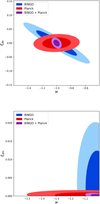Fig. 15. Marginalized constraints (68% and 95% CL) for two interacting dark energy models with Q ∝ ρde and w < −1 (top) or Q ∝ ρdm (bottom) from BINGO, Planck, and BINGO + Planck.

Our results show that BINGO can put a better constraint on the interaction parameter ξ_de than Planck for the model with Q ∝ ρ_de and w > −1. However, the constraint on the DE EoS is weakened. If w < −1, we do not observe appreciable difference in our H I Fisher matrix compared with the previous case, but Planck possesses better constraints for both the DE EoS and the interaction parameter. In general, the combination with Planck yields results of δw ∼ 5% and σ_ξde ∼ 0.02 for Q ∝ ρ_de. If the interaction is proportional to the DM energy density, BINGO and Planck have opposite behaviors, with BINGO providing tighter constraints on the DE EoS, but allowing a wider uncertainty in the interaction, and Planck having looser constraints on the EoS, but tight contours for the interaction parameter. This is expected, as shown in Fig. 1 of Costa et al. (2019) where the BAO scale is more affected by the interaction at higher redshifts, and was also obtained in Table 10 of Costa et al. (2017) comparing low-redshift data with Planck data. Finally, the combination of the two surveys greatly improves the cosmological constraints. We summarize our results in Table 11.

Projected constraints with H I IM experiments for interacting DE models were also considered in Xu et al. (2018). Their result for BINGO, however, could be about ten times stronger for the DE EoS and about four times stronger for the interacting parameter under the model with Q ∝ ρ_de and w > −1. Although there are some differences in the BINGO setup, we were only able to obtain this level of constraint in combination with Planck data.

5. Conclusions

BINGO will be a single-dish radio telescope designed to observe the LSS using H I intensity mapping as a tracer of the underlying matter distribution. Therefore, it will provide additional data, susceptible to different systematic effects, that can help improve our current understanding of the late-time cosmological expansion and structure formation. In this work we used the 21 cm angular power spectra and the Fisher matrix formalism to forecast the constraining power of BINGO on standard and alternative cosmological models, and analyzed the dependency with different instrument configurations. In summary, we obtained the following:

• If we assume the ΛCDM model, the fiducial BINGO setup (see Table 2) cannot put competitive constraints on Planck. However, their combination can improve the confidence in all cosmological parameters; the Hubble constant and the DM parameter (Ω_ch²) are the most significant with an improvement of ∼25% in both. This is competitive with current combined constraints from CMB and BAO data.

• BINGO plays a more significant role if we leave the DE EoS as a free parameter. In the wCDM model, BINGO alone can establish better constraints than Planck for the EoS. Their combination can reach 1.1% precision for H₀ and 3.3% for w at 68% CL, which have improved by respectively 92% and 87% in comparison with Planck alone.

• Under the CPL parameterization, BINGO + Planck achieves a 2.9% precision in the Hubble constant, 30% in the DE parameter w₀, and σ_wa = 1.2 for w_a at one standard deviation. Although these constraints can be considered large, BINGO has improved the constraints from Planck alone by up to 78%.

• Fixing the CPL parameterization as our fiducial cosmological model, we considered how the cosmological constraints should be affected by several different instrumental scenarios: Total observational time: We considered the impact of the total observational time on our cosmological constraints, which affects the thermal noise level of our experiment. We observe that BINGO will mainly affect the constraints on the Hubble constant and the DE EoS. A five-year experiment can improve these constraints by δσ_H0 = 25%, δσ_w0 and δσ_wa ∼ 21% compared to the one-year survey. The FoM defined by the error ellipsoid improved by 11 times for BINGO only and 2.7 times in combination with Planck. Although our constraints have improved for longer total observational time, they significantly flatten after three years, suggesting this as an optimal observational time. Number of feed horns: The fiducial setup assumes 28 feed horns. Considering the effect on the noise level only, increasing the number of horns to a maximum value of 60 can improve the constraints by at most 10%. Given the costs necessary to increase the number of horns and its connection with the total observational time, it may be more significant to increase the number of horns in such way to cover a larger area in the sky. Number of redshift bins: The constraints are significantly affected by the number of bins considered; however, we observe small deviations from N_bin = 64 to N_bin = 128, suggesting that we have reached a plateau. As the actual number of redshift bins in the raw data of BINGO will be much larger, this choice must take into account the necessary computational calculations. Our analysis suggests that N_bin = 64 is optimal. Cross-correlations: Some previous analysis considered the Limber approximation to extract the 21 cm information. We analyzed the effect of including all the spectra on the final constraints. The importance of cross-correlations increases as we increase the number of bins, but eventually reaches a plateau. For N_bin = 32, near BINGO standard configuration, we obtain improvements of δln(10¹⁰A_s) = 0.4%, δΩ_bh² = 6.8%, δn_s = 7.2%, δh = 8.3%, δw₀ = 8.8%, δw_a = 11%, δΩ_ch² = 22%, and δb_H I = 31%. RSD: RSD can break the degeneracy between A_s and b_H I and improve the constraints on the other cosmological parameters. At N_bin = 128 the improvements from RSD are given by δh = 1%, δln(10¹⁰A_s) = 2.2%, δΩ_bh² = 7.8%, δn_s = 9.5%, δw₀ = 14%, δw_a = 34%, δΩ_ch² = 44%, and δb_H I = 176%, combining BINGO with Planck data. Foreground residuals: Foreground residuals will both increase the statistical errors and introduce biases in our final cosmological parameter estimation. We take these effects into account assuming that some sort of foreground removal technique has already been accomplished, and model the residual contamination as the sum of Gaussian processes. We obtain that the statistical error bars are not strongly enhanced; the maximum degradation was of 16% for BINGO only and 6% for BINGO + Planck with the overall scaling factor ϵ_FG = 1 (no foreground removal). On the other hand, we found that the bias in our cosmological constraints will be at maximum 1σ if ϵ_FG = 10⁻⁴, and can be significantly smaller if we can achieve smaller values for ϵ_FG.

• We also compared the BINGO constraints to those from SKA1-MID band 1 and SKA1-MID band 2. Given the larger surveyed area, deeper redshift range, larger number of antennas, and lower system temperature, BINGO cannot compete with them. However, SKA will have more complicated systematic effects and BINGO can be a pathfinder to better understand them.

• In addition to our cosmological parameters, BINGO will help us understand the H I evolution and distribution. This is affected by the cosmological model and the H I model considered. Combining BINGO and Planck data, we obtained a 2.3% precision fixing the H I density parameter under the CPL parameterization. Our worst scenario is obtained assuming that Ω_H I and b_H I vary with redshift as a free parameter over three groups of redshift bins. In this case we have ${\sigma }_{{\mathrm{\Omega }}_{\mathrm{H}\mathrm{I}}^i}\sim 8.5\%$ and ${\sigma }_{b_{\mathrm{H}\mathrm{I}}^i}\sim 6\%$.

• Measurements from the H I power spectrum can break the geometric degeneracy in the parameter space of ΛCDM + ∑m_ν. In combination with BINGO, we obtained σ_∑mν < 0.14 eV at 95% CL, which is on the same order of current constraints.

• BINGO can also help constrain alternative cosmological models breaking degeneracies in the parameter space. In particular, under the B₀-parameterization of f(R) gravity, we obtained σ_B0 = 3.1 × 10⁻⁵ with BINGO against σ_B0 = 5.3 × 10⁻² from Planck. On the other hand, we forecast that BINGO + Planck will be able to put constraints of σ_ξde ∼ 0.02 and σ_ξdm = 0.0007 on the interacting dark energy parameters.

We would like to note some limitations and future extensions of the present work:

• First, we considered the full 21 cm angular power spectrum. Although this has more information than the BAO data alone, it is also more contaminated by the H I physics.

• In our analysis we used the Fisher matrix formalism. It is well known that the Fisher matrix produces the optimal scenario, thus we should expect deviations from the present constraints in a more robust MCMC sampling of the parameter space through the 21 cm likelihood. Because of the tomographic nature of our 21 cm angular spectra, spanning a 3D volume, the number of necessary computations can increase dramatically compared to the CMB angular spectra. Therefore, given our computational resources at the moment, we decided to adopt the Fisher matrix formalism, which has been widely used in the literature to forecast cosmological constraints and can provide consistent results.

• As discussed before, BINGO will be mainly affected by the presence of foregrounds. Here the bulk of our analysis considers a perfect foreground removal technique. Of course, this will not be the case, and foreground residuals must be taken into account. In the BINGO companion papers (Liccardo et al. 2022; Fornazier et al. 2022), the foreground cleaning process is further discussed.

• The real situation will also be contaminated by other effects. The 1/f noise will be the most prominent of them for the BINGO configuration. Other effects that must be taken into account in the final analysis include standing waves, side lobes, RFI, and atmospheric effects.

• Although BINGO’s beam resolution will suppress most nonlinear effects, very thin redshift bins can have a significant contribution from nonlinearities. Nonlinear effects are further discussed in our BINGO companion paper (Zhang et al. 2022) and their impact on the cosmological parameters will be analyzed in a future work.

Acknowledgments

The BINGO project is supported by FAPESP grant 2014/07885-0; the support from CNPq is also gratefully acknowledged (E.A.). A.A.C. acknowledges financial support from the China Postdoctoral Science Foundation, grant number 2020M671611. R.G.L. thanks CAPES (process 88881.162206/2017-01) and the Alexander von Humboldt Foundation for the financial support. C.P.N. would like to thank São Paulo Research Foundation (FAPESP), grant 2019/06040-0, for financial support. F.B.A. acknowledges the UKRI-FAPESP grant 2019/05687-0, and FAPESP and USP for Visiting Professor Fellowships where this work has been developed. B.W. and A.A.C. were also supported by the key project of NNSFC under grant 11835009. C.A.W. acknowledges a CNPq grant 2014/313.597. T.V. acknowledges CNPq Grant 308876/2014-8. K.S.F.F. would like to thank FAPESP for financial support grant 2017/21570-0. A.R.Q., F.A.B., L.B. and M.V.S. acknowledge PRONEX/CNPq/FAPESQ-PB (Grant no. 165/2018). V.L. would like to thank São Paulo Research Foundation (FAPESP), grant 2018/02026-0, for financial support. L.S. is supported by the National Key R&D Program of China (2020YFC2201600). J.Z. was supported by IBS under the project code, IBS-R018-D1. We thank an anonymous referee for his/her very insightful comments.

References

Appendix A: Code comparison

In order to check the outputs of the code used throughout this work, we show here a comparison between the C_ℓ values (and their derivatives) calculated using this code and those obtained from the Unified Cosmological Library for C_ℓs code (UCLCL; McLeod et al. 2017; Loureiro et al. 2019), matching cosmologies as closely as possible. UCLCL uses the power spectra and transfer functions from the CLASS code (Blas et al. 2011) to construct the angular power spectrum C_ℓ,

$$\begin{array}{c}\hfill C_{\ell }^{\mathit{ij}}=\frac{2}{\pi }{\displaystyle \int }{W}_{\ell }^i(k)W_{\ell }^j(k)k^{2}P(k)dk,\end{array}$$(A.1)

where the indices i and j denote the different redshift bins, P(k) is the underlying matter density field power spectrum at zero redshift, and W_ℓ(k) is the window function that accounts for projection effects and all the processes involved in the evolution, including RSD (see discussion in Loureiro et al. 2019).

We set the cosmological parameters to the most recent Planck results for ΛCDM as fiducial values (Ω_bh² = 0.0224, Ω_ch² = 0.120, h = 0.673, Ω_kh² = 0, w₀ = −1, w_a = 0, n_s = 0.965, ln(10¹⁰A_s) = 3.096; Planck Collaboration VI 2020).

We performed several tests and comparisons, and here we present a set of them as illustrative examples in order to give the overall picture of the level of agreement among the results of each code. We first compared the results obtained for a total of 30 frequency bands, each with 10 MHz bandwidths, covering the BINGO frequency range. Some examples of the resulting auto- and cross-correlation spectra are shown in the upper panel of Figs. A.1 and A.2, respectively. The lower panel in each figure presents the respective relative difference, in percentage, and shows that the codes deviate from each other by less than 1% for the auto-$C_{\mathcal{l}}^{ij}$s and less than 2% for the cross-$C_{\mathcal{l}}^{ij}$s at multipoles up to ℓ ∼ 100. A larger discrepancy for higher multipoles is introduced not only by small numerical errors (characterized by the noisy behavior), but mainly because the $C_{\mathcal{l}}^{ij}$s have very small absolute values at this region, reaching zero, especially in the case of cross-correlation. This is evident from the blue line in Fig. A.2, representing the cross-correlation among the frequency bins centered at 1105 MHz and 1085 MHz, which present $C_{\mathcal{l}}^{ij}$ values near zero at the first multipoles (upper panel), resulting in a larger relative difference at these multipoles as well (lower panel).

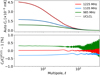Fig. A.1. Comparison between the auto-correlation $C_{\mathcal{l}}^{ij}$s (for i = j) calculated in this work and those obtained with the UCLCL code at three BINGO redshift bins, centered at the frequencies 985, 1105, and 1225 MHz (redshifts z ≈ 0.44, 0.28, and 0.16, respectively), and bandwidths of 10 MHz. The upper panel shows the UCLCL results overplotted as dotted lines on each of the calculated curves (colored lines), while the lower panel shows the percentage relative difference among them.

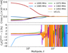Fig. A.2. Same as Fig. A.1, but for the cross-correlation $C_{\mathcal{l}}^{ij}$s (i ≠ j) between the frequency bin centered at 1105 MHz (z = 0.28) and the five following frequency bins, with bandwidth of 10 MHz.

We also investigated the influence of different bandwidths when comparing the codes. We tested four bandwidths (2 MHz, 10 MHz, 35 MHz and 75 MHz) centered at the frequency of 1110 MHz. The comparison among some of the auto-$C_{\mathcal{l}}^{ij}$s resulting from each code is depicted in Fig. A.3. Again, the level of agreement is better than 99.5% for the thinner bandwidths, while it reaches 99% for the thicker bandwidth, showing that the smaller the bandwidth the better the level of agreement between the codes.

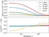Fig. A.3. Comparison between the auto-correlation $C_{\mathcal{l}}^{ij}$s calculated in this work and using the UCLCL code for four different bandwidths between 2 and 75 MHz, all of them centered at a frequency of 1110 MHz. Again, the upper panel shows the results overplotted and the lower panel shows the percentage difference among them.

Finally, we compared the two codes in the context of the derivatives of the $C_{\mathcal{l}}^{ij}$s with respect to a set of cosmological and 21 cm parameters, calculated with a variation of 1% on the corresponding fiducial values. The comparison, presented in Fig. A.4 for a bandwidth of 10 MHz centered at 1110 MHz, shows an agreement of more than 99%, for all parameters considered, for multipoles up to ℓ ∼ 100, and of more than 98% for larger multipoles. The same comparison was performed for other different bandwidths, obtaining results similar to those observed in Fig. A.4 for bandwidths of 2 MHz and 35 MHz, and a larger discrepancy for the broader band, 75 MHz, but still following the expected from Fig. A.3.

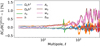Fig. A.4. Percentage relative difference comparing the derivatives, $\delta C_{\mathcal{l}}^{ij}=d{C}_{\mathcal{l}}^{ij}/dx$ (for auto-correlation, i = j), with x representing each cosmological and 21 cm parameter, calculated in this work and by using the UCLCL code. All the cases correspond to a frequency channel with a bandwidth of 10 MHz centered at 1110 MHz.

All Tables

All Figures

Fig. 1. Brightness temperature perturbation power spectrum at z = 0.13 (solid lines) and z = 0.45 (dashed lines) with a 9.33 MHz bandwidth. The auto-spectra of the full signal (black) and of each individual term are shown, generically grouped as Newtonian-gauge density (red), redshift-space distortions (green), velocity term (blue), all potential terms evaluated at the source position (cyan), and the ISW component (magenta). The power spectrum is dominated by the H I overdensity at small scales and has a significant contribution from RSD at large scales.

In the text

Fig. 2. Fractional uncertainties expected for the angular power spectrum for the BINGO experiment (fsky = 0.07) for redshifts z = 0.127 (solid lines) and z = 0.449 (dashed lines) after 1 year of sky integration. The ratio is plotted between different sources of uncertainty (cosmic variance, shot noise, and thermal noise) and the H I angular power spectrum, $\mathrm{\Delta }{C}_{\ell }/C_{\ell }^{\mathrm{H}\mathrm{I}}$, as a function of multipole. For the cosmic variance the standard formula, $\sqrt{2/(2\ell +1)f_{\mathrm{sky}}}$, is used, and for the thermal and shot noise ΔCℓ is equal to their angular power spectrum multiplied by the cosmic variance factor.

In the text

	Fig. 3. Marginalized constraints (68% and 95% CL) on the DE EoS and Hubble parameters for the wCDM model using BINGO, Planck, and BINGO + Planck.
In the text

	Fig. 4. Marginalized constraints (68% and 95% CL) on the DE EoS parameters for the CPL parameterization using BINGO, Planck, and BINGO + Planck.
In the text

	Fig. 5. Constraints on the cosmological and H I parameters as a function of the total observational time relative to those with tobs = 1 year for BINGO (top) and BINGO + Planck (bottom). We vary tobs in a range of [1,  2,  3,  4,  5] years. In the bottom plot wa is on top of w0, which cannot be seen.
In the text

	Fig. 6. Constraints on the cosmological and H I parameters as a function of the number of feed horns for BINGO + Planck.
In the text

	Fig. 7. Projected constraints on the cosmological and H I parameters as a function of the number of bins for BINGO (top) and BINGO + Planck (bottom). They show that w0, wa, and h can have their constraints further improved for Nbin > 30.
In the text

	Fig. 8. Percentage difference between using and not using information from the cross-correlations in the projected cosmological parameter constraints expected for BINGO + Planck.
In the text

	Fig. 9. Percentage difference between using and not using information from RSD in the cosmological parameter constraints from BINGO (top) and BINGO + Planck (bottom).
In the text

	Fig. 10. Marginalized statistical errors as a function of the residual foreground contamination amplitude, ϵFG, from BINGO (top) and BINGO + Planck (bottom).
In the text

	Fig. 11. Ratio of bias to the marginalized statistical errors for each parameter as a function of the residual foreground contamination amplitude, ϵFG, from BINGO (top) and BINGO + Planck (bottom).
In the text

	Fig. 12. Marginalized constraints (68% and 95% CL) on the DE EoS parameters for the CPL parameterization with BINGO, considering the effect of foreground residuals on the statistical and systematic errors. The star corresponds to our fiducial value and the cross shows the value recovered given the Fisher matrix bias. We have fixed ϵFG = 10−4.
In the text

	Fig. 13. One- and two-dimensional (68% and 95% CL) cosmological constraints for a CPL parameterization from BINGO, SKA1-MID band 1, and SKA1-MID band 2 in combination with Planck data. This illustrates that BINGO can be considered a pathfinder for constraints obtained by SKA.
In the text

	Fig. 14. Marginalized constraints (68% and 95%) CL on the modified gravity parameter B0 and the Hubble parameter from BINGO, Planck, and BINGO + Planck.
In the text

	Fig. 15. Marginalized constraints (68% and 95% CL) for two interacting dark energy models with Q ∝ ρde and w < −1 (top) or Q ∝ ρdm (bottom) from BINGO, Planck, and BINGO + Planck.
In the text

Fig. A.1. Comparison between the auto-correlation $C_{\mathcal{l}}^{ij}$s (for i = j) calculated in this work and those obtained with the UCLCL code at three BINGO redshift bins, centered at the frequencies 985, 1105, and 1225 MHz (redshifts z ≈ 0.44, 0.28, and 0.16, respectively), and bandwidths of 10 MHz. The upper panel shows the UCLCL results overplotted as dotted lines on each of the calculated curves (colored lines), while the lower panel shows the percentage relative difference among them.

In the text

	Fig. A.2. Same as Fig. A.1, but for the cross-correlation $C_{\mathcal{l}}^{ij}$s (i ≠ j) between the frequency bin centered at 1105 MHz (z = 0.28) and the five following frequency bins, with bandwidth of 10 MHz.
In the text

	Fig. A.3. Comparison between the auto-correlation $C_{\mathcal{l}}^{ij}$s calculated in this work and using the UCLCL code for four different bandwidths between 2 and 75 MHz, all of them centered at a frequency of 1110 MHz. Again, the upper panel shows the results overplotted and the lower panel shows the percentage difference among them.
In the text

	Fig. A.4. Percentage relative difference comparing the derivatives, $\delta C_{\mathcal{l}}^{ij}=d{C}_{\mathcal{l}}^{ij}/dx$ (for auto-correlation, i = j), with x representing each cosmological and 21 cm parameter, calculated in this work and by using the UCLCL code. All the cases correspond to a frequency channel with a bandwidth of 10 MHz centered at 1110 MHz.
In the text

References

- Abbott, T. M. C., Aguena, M., Alarcon, A., et al. 2021, Phys. Rev. D, 105, 023520 [Google Scholar]
- Abdalla, E., & Marins, A. 2020, Int. J. Mod. Phys. D, 29, 2030014 [NASA ADS] [CrossRef] [Google Scholar]
- Abdalla, E., Ferreira, E. G. M., Landim, R. G., et al. 2022a, A&A, 664, A14 (Paper I) [NASA ADS] [CrossRef] [EDP Sciences] [Google Scholar]
- Abdalla, F. B., Marins, A., Motta, P., et al. 2022b, A&A, 664, A16 (Paper III) [NASA ADS] [CrossRef] [EDP Sciences] [Google Scholar]
- Ahmad, Q. R., et al. (SNO Collaboration) 2002, Phys. Rev. Lett., 89, 011301 [NASA ADS] [CrossRef] [Google Scholar]
- Albrecht, A., Bernstein, G., Cahn, R., et al. 2006, ArXiv e-prints [arXiv:astro-ph/0609591] [Google Scholar]
- Amara, A., & Refregier, A. 2008, MNRAS, 391, 228 [NASA ADS] [CrossRef] [Google Scholar]
- Amendola, L. 2000, Phys. Rev. D, 62, 043511 [NASA ADS] [CrossRef] [Google Scholar]
- Bacon, D. J., Battye, R. A., Bull, P., et al. 2020, PASA, 37, e007 [NASA ADS] [CrossRef] [Google Scholar]
- Bandura, K., Addison, G. E., Amiri, M., et al. 2014, Proc. SPIE Int. Soc. Opt. Eng., 9145, 22 [Google Scholar]
- Battye, R. A., Davies, R. D., & Weller, J. 2004, MNRAS, 355, 1339 [NASA ADS] [CrossRef] [Google Scholar]
- Battye, R. A., Brown, M. L., Browne, I. W. A., et al. 2012, ArXiv e-prints [arXiv:1209.1041] [Google Scholar]
- Battye, R., Browne, I., Dickinson, C., et al. 2013, MNRAS, 434, 1239 [NASA ADS] [CrossRef] [Google Scholar]
- Battye, R., Browne, I., Chen, T., et al. 2016, ArXiv e-prints [arXiv:1610.06826] [Google Scholar]
- Bigot-Sazy, M. A., Dickinson, C., Battye, R., et al. 2015, MNRAS, 454, 3240 [NASA ADS] [CrossRef] [Google Scholar]
- Blas, D., Lesgourgues, J., & Tram, T. 2011, JCAP, 2011, 034 [Google Scholar]
- Bull, P., Ferreira, P. G., Patel, P., & Santos, M. G. 2015, ApJ, 803, 21 [NASA ADS] [CrossRef] [Google Scholar]
- Chang, T.-C., Pen, U.-L., Peterson, J. B., & McDonald, P. 2008, Phys. Rev. Lett., 100, 091303 [NASA ADS] [CrossRef] [Google Scholar]
- Chang, T.-C., Pen, U.-L., Bandura, K., & Peterson, J. B. 2010, Nature, 466, 463 [Google Scholar]
- Chen, X. 2012, Int. J. Mod. Phys. Conf. Ser., 12, 256 [NASA ADS] [CrossRef] [Google Scholar]
- Chen, T., Battye, R., Costa, A., Dickinson, C., & Harper, S. 2020, MNRAS, 491, 4254 [NASA ADS] [CrossRef] [Google Scholar]
- Chevallier, M., & Polarski, D. 2001, Int. J. Mod. Phys. D, 10, 213 [Google Scholar]
- Clifton, T., Ferreira, P. G., Padilla, A., & Skordis, C. 2012, Phys. Rep., 513, 1 [NASA ADS] [CrossRef] [Google Scholar]
- Copeland, E. J., Sami, M., & Tsujikawa, S. 2006, Int. J. Mod. Phys. D, 15, 1753 [NASA ADS] [CrossRef] [Google Scholar]
- Costa, A. A., Xu, X.-D., Wang, B., Ferreira, E. G. M., & Abdalla, E. 2014, Phys. Rev. D, 89, 103531 [NASA ADS] [CrossRef] [Google Scholar]
- Costa, A. A., Olivari, L. C., & Abdalla, E. 2015, Phys. Rev. D, 92, 103501 [NASA ADS] [CrossRef] [Google Scholar]
- Costa, A. A., Xu, X.-D., Wang, B., & Abdalla, E. 2017, JCAP, 01, 028 [CrossRef] [Google Scholar]
- Costa, A. A., Marcondes, R. J. F., Landim, R. G., et al. 2019, MNRAS, 488, 78 [NASA ADS] [CrossRef] [Google Scholar]
- Daniel, S. F., Linder, E. V., Smith, T. L., et al. 2010, Phys. Rev. D, 81, 123508 [NASA ADS] [CrossRef] [Google Scholar]
- Deffayet, C., Gao, X., Steer, D. A., & Zahariade, G. 2011, Phys. Rev. D, 84, 064039 [NASA ADS] [CrossRef] [Google Scholar]
- Feng, C., Wang, B., Abdalla, E., & Su, R.-K. 2008, Phys. Lett. B, 665, 111 [NASA ADS] [CrossRef] [Google Scholar]
- Ferreira, E. G., Quintin, J., Costa, A. A., Abdalla, E., & Wang, B. 2017, Phys. Rev. D, 95, 043520 [NASA ADS] [CrossRef] [Google Scholar]
- Fornazier, K. S. F., Abdalla, F. B., Remazeilles, M., et al. 2022, A&A, 664, A18 (Paper V) [NASA ADS] [CrossRef] [EDP Sciences] [Google Scholar]
- Fukuda, Y., et al. (Super-Kamiokande Collaboration) 1998, Phys. Rev. Lett., 81, 1562 [NASA ADS] [CrossRef] [Google Scholar]
- Furlanetto, S., Oh, S., & Briggs, F. 2006, Phys. Rep., 433, 181 [NASA ADS] [CrossRef] [Google Scholar]
- Gavela, M. B., Hernandez, D., Lopez Honorez, L., Mena, O., & Rigolin, S. 2009, JCAP, 0907, 034 [Erratum: JCAP 1005, E01 (2010)] [CrossRef] [Google Scholar]
- Giannantonio, T., Martinelli, M., Silvestri, A., & Melchiorri, A. 2010, JCAP, 04, 030 [CrossRef] [Google Scholar]
- Hall, A., Bonvin, C., & Challinor, A. 2013, Phys. Rev. D, 87, 064026 [NASA ADS] [CrossRef] [Google Scholar]
- Harper, S. E., & Dickinson, C. 2018, MNRAS, 479, 2024 [NASA ADS] [CrossRef] [Google Scholar]
- Harper, S., Dickinson, C., Battye, R., et al. 2018, MNRAS, 478, 2416 [NASA ADS] [CrossRef] [Google Scholar]
- He, J.-H., Wang, B., & Abdalla, E. 2009, Phys. Lett. B, 671, 139 [NASA ADS] [CrossRef] [Google Scholar]
- He, J.-H., Wang, B., & Abdalla, E. 2011, Phys. Rev. D, 83, 063515 [NASA ADS] [CrossRef] [Google Scholar]
- Hildebrandt, H., Köhlinger, F., van den Busch, J. L., et al. 2020, A&A, 633, A69 [NASA ADS] [CrossRef] [EDP Sciences] [Google Scholar]
- Hojjati, A., Pogosian, L., Silvestri, A., & Talbot, S. 2012, Phys. Rev. D, 86, 123503 [NASA ADS] [CrossRef] [Google Scholar]
- Horndeski, G. W. 1974, Int. J. Theor. Phys., 10, 363 [NASA ADS] [CrossRef] [Google Scholar]
- Hu, W., & Sawicki, I. 2007, Phys. Rev. D, 76, 064004 [CrossRef] [Google Scholar]
- Kerp, J., Winkel, B., Ben Bekhti, N., Floeer, L., & Kalberla, P. 2011, Astron. Nachr., 332, 637 [NASA ADS] [CrossRef] [Google Scholar]
- Koyama, K., Maartens, R., & Song, Y.-S. 2009, JCAP, 0910, 017 [CrossRef] [Google Scholar]
- Landim, R. G., & Abdalla, E. 2017, Phys. Lett. B, 764, 271 [NASA ADS] [CrossRef] [Google Scholar]
- Landim, R. G., Marcondes, R. J. F., Bernardi, F. F., & Abdalla, E. 2018, Braz. J. Phys., 48, 364 [NASA ADS] [CrossRef] [Google Scholar]
- Lesgourgues, J., & Pastor, S. 2012, Adv. High Energy Phys., 2012, 608515 [CrossRef] [Google Scholar]
- Lewis, A., & Bridle, S. 2002, Phys. Rev. D, 66, 103511 [Google Scholar]
- Liccardo, V., de Mericia, E. J., Wuensche, C. A., et al. 2022, A&A, 664, A17 (Paper IV) [NASA ADS] [CrossRef] [EDP Sciences] [Google Scholar]
- Linder, E. V. 2003, Phys. Rev. Lett., 90, 091301 [Google Scholar]
- Loeb, A., & Wyithe, S. 2008, Phys. Rev. Lett., 100, 161301 [NASA ADS] [CrossRef] [Google Scholar]
- Loureiro, A., Moraes, B., Abdalla, F. B., et al. 2019, MNRAS, 485, 326 [NASA ADS] [CrossRef] [Google Scholar]
- Maino, D., Burigana, C., Maltoni, M., et al. 1999, A&AS, 140, 383 [NASA ADS] [CrossRef] [EDP Sciences] [Google Scholar]
- Marcondes, R. J., Landim, R. C., Costa, A. A., Wang, B., & Abdalla, E. 2016, JCAP, 12, 009 [CrossRef] [Google Scholar]
- Masui, K. W., Schmidt, F., Pen, U.-L., & McDonald, P. 2010, Phys. Rev. D, 81, 062001 [NASA ADS] [CrossRef] [Google Scholar]
- Masui, K. W., Switzer, E. R., Banavar, N., et al. 2013, ApJ, 763, L20 [Google Scholar]
- McLeod, M., Balan, S. T., & Abdalla, F. B. 2017, MNRAS, 466, 3558 [NASA ADS] [CrossRef] [Google Scholar]
- Meinhold, P., Leonardi, R., Aja, B., et al. 2009, J. Instrum., 12, T12009 [CrossRef] [Google Scholar]
- Micheletti, S., Abdalla, E., & Wang, B. 2009, Phys. Rev. D, 79, 123506 [NASA ADS] [CrossRef] [Google Scholar]
- Nan, R., Li, D., Jin, C., et al. 2011, Int. J. Mod. Phys. D, 20, 989 [Google Scholar]
- Olivari, L., Remazeilles, M., & Dickinson, C. 2016, MNRAS, 456, 2749 [NASA ADS] [CrossRef] [Google Scholar]
- Olivari, L. C., Dickinson, C., Battye, R. A., et al. 2018, MNRAS, 473, 4242 [Google Scholar]
- Perlmutter, S., Aldering, G., Goldhaber, G., et al. 1999, ApJ, 517, 565 [Google Scholar]
- Planck Collaboration VI. 2020, A&A, 641, A6 [NASA ADS] [CrossRef] [EDP Sciences] [Google Scholar]
- Pritchard, J. R., & Loeb, A. 2012, Rept. Prog. Phys., 75, 086901 [NASA ADS] [CrossRef] [Google Scholar]
- Pu, B.-Y., Xu, X.-D., Wang, B., & Abdalla, E. 2015, Phys. Rev. D, 92, 123537 [NASA ADS] [CrossRef] [Google Scholar]
- Remazeilles, M., Delabrouille, J., & Cardoso, J.-F. 2011a, MNRAS, 410, 2481 [Google Scholar]
- Remazeilles, M., Delabrouille, J., & Cardoso, J.-F. 2011b, MNRAS, 418, 467 [Google Scholar]
- Riess, A. G., Filippenko, A. V., Challis, P., et al. 1998, AJ, 116, 1009 [Google Scholar]
- Riess, A. G., Casertano, S., Yuan, W., Macri, L. M., & Scolnic, D. 2019, ApJ, 876, 85 [Google Scholar]
- Rohlfs, K., & Wilson, T. 2004, Tools of Radio Astronomy (Berlin, Heidelberg: Springer-Verlag), 16 [CrossRef] [Google Scholar]
- Santos, M. G., Cooray, A., & Knox, L. 2005, ApJ, 625, 575 [NASA ADS] [CrossRef] [Google Scholar]
- Santos, M. G., Bull, P., Alonso, D., et al. 2015, Proceedings of Advancing Astrophysics with the Square Kilometre Array (AASKA14), 9-13 June, 2014. Giardini Naxos, Italy, id.19 [Google Scholar]
- Seiffert, M., Mennella, A., Burigana, C., et al. 2002, A&A, 391, 1185 [NASA ADS] [CrossRef] [EDP Sciences] [Google Scholar]
- Sethi, S. K. 2005, MNRAS, 363, 818 [NASA ADS] [CrossRef] [Google Scholar]
- Switzer, E. R., Masui, K. W., Bandura, K., et al. 2013, MNRAS, 434, L46 [NASA ADS] [CrossRef] [Google Scholar]
- Tegmark, M., Taylor, A., & Heavens, A. 1997, ApJ, 480, 22 [NASA ADS] [CrossRef] [Google Scholar]
- Valiviita, J., Majerotto, E., & Maartens, R. 2008, JCAP, 0807, 020 [CrossRef] [Google Scholar]
- Visbal, E., Loeb, A., & Wyithe, J. B. 2009, JCAP, 10, 030 [CrossRef] [Google Scholar]
- Wang, B., Abdalla, E., Atrio-Barandela, F., & Pavon, D. 2016, Rep. Prog. Phys., 79, 096901 [NASA ADS] [CrossRef] [Google Scholar]
- Wetterich, C. 1995, A&A, 301, 321 [NASA ADS] [Google Scholar]
- Wilson, T., Rohlfs, K., & Huettemeister, S. 2013, Tools of Radio Astronomy, 6th edn. (Berlin, Heidelberg: Springer-Verlag) [CrossRef] [Google Scholar]
- Wuensche, C. A., & the BINGO Collaboration 2019, J. Phys. Conf. Ser., 1269, 012002 [NASA ADS] [CrossRef] [Google Scholar]
- Wuensche, C. A., Villela, T., Abdalla, E., et al. 2022, A&A, 664, A15 (Paper II) [NASA ADS] [CrossRef] [EDP Sciences] [Google Scholar]
- Xiao, L., Costa, A. A., & Wang, B. 2021, MNRAS, 510, 1495 [NASA ADS] [CrossRef] [Google Scholar]
- Xu, X., Ma, Y.-Z., & Weltman, A. 2018, Phys. Rev. D, 97, 083504 [NASA ADS] [CrossRef] [Google Scholar]
- Yohana, E., Li, Y.-C., & Ma, Y.-Z. 2019, Res. Astron. Astrophys., 19, 186 [CrossRef] [Google Scholar]
- Zhang, J., Motta, P., Novaes, C. P., et al. 2022, A&A, 664, A19 (Paper VI) [NASA ADS] [CrossRef] [EDP Sciences] [Google Scholar]