| Issue |
A&A
Volume 666, October 2022
|
|
|---|---|---|
| Article Number | A83 | |
| Number of page(s) | 17 | |
| Section | Cosmology (including clusters of galaxies) | |
| DOI | https://doi.org/10.1051/0004-6361/202243158 | |
| Published online | 10 October 2022 | |
The BINGO project
VIII. Recovering the BAO signal in HI intensity mapping simulations
1
Instituto Nacional de Pesquisas Espaciais, Av. dos Astronautas 1758, Jardim da Granja, São José dos Campos, SP, Brazil
e-mail: This email address is being protected from spambots. You need JavaScript enabled to view it.
, This email address is being protected from spambots. You need JavaScript enabled to view it.
2
Shanghai Astronomical Observatory, Chinese Academy of Sciences, Shanghai 200030, PR China
3
University College London, Gower Street, London WC1E 6BT, UK
4
Instituto de Física, Universidade de São Paulo, R. do Matão, 1371 – Butantã, 05508-09 São Paulo, SP, Brazil
5
Department of Physics and Electronics, Rhodes University, PO Box 94 Grahamstown 6140, South Africa
6
CNRS-UCB International Research Laboratory, Centre Pierre Binétruy, IRL2007, CPB-IN2P3, Berkeley, USA
7
Laboratoire Astroparticule et Cosmologie (APC), CNRS/IN2P3, Université Paris Diderot, 75205 Paris Cedex 13, France
8
IRFU, CEA, Université Paris-Saclay, 91191 Gif-sur-Yvette, France
9
Department of Astronomy, School of Physical Sciences, University of Science and Technology of China, Hefei, Anhui 230026, PR China
10
Instituto de Física de Cantabria (CSIC-Universidad de Cantabria), Avda. de los Castros s/n, 39005 Santander, Spain
11
Jodrell Bank Centre for Astrophysics, Department of Physics and Astronomy, The University of Manchester, Oxford Road, Manchester M13 9PL, UK
12
Center for Gravitation and Cosmology, College of Physical Science and Technology, Yangzhou University, Yangzhou 225009, PR China
13
School of Aeronautics and Astronautics, Shanghai Jiao Tong University, Shanghai 200240, PR China
14
Technische Universität München, Physik-Department T70, James-Franck-Strasse 1, 85748 Garching, Germany
15
Unidade Acadêmica de Física, Universidade Federal de Campina Grande, R. Aprígio Veloso, Bodocongó, 58429-900 Campina Grande, PB, Brazil
16
Centro de Gestão e Estudos Estratégicos SCS Qd 9, Lote C, Torre C S/N Salas 401 a 405, 70308-200 Brasília, DF, Brazil
17
Instituto de Física, Universidade de Brasília, Campus Universitário Darcy Ribeiro, 70910-900 Brasília, DF, Brazil
18
College of Science, Nanjing University of Aeronautics and Astronautics, Nanjing 211106, PR China
19
Kavli IPMU (WPI), UTIAS, The University of Tokyo, 5-1-5 Kashiwanoha, Kashiwa, Chiba 277-8583, Japan
Received:
19
January
2022
Accepted:
29
July
2022
Abstract
Context. A new and promising technique for observing the Universe and study the dark sector is the intensity mapping of the redshifted 21 cm line of neutral hydrogen (H I). The Baryon Acoustic Oscillations [BAO] from Integrated Neutral Gas Observations (BINGO) radio telescope will use the 21 cm line to map the Universe in the redshift range 0.127 ≤ z ≤ 0.449 in a tomographic approach, with the main goal of probing the BAO.
Aims. This work presents the forecasts of measuring the transversal BAO signal during the BINGO phase 1 operation.
Methods. We used two clustering estimators: the two-point angular correlation function (ACF) in configuration space, and the angular power spectrum (APS) in harmonic space. We also used a template-based method to model the ACF and APS estimated from simulations of the BINGO region and to extract the BAO information. The tomographic approach allows the combination of redshift bins to improve the template fitting performance. We computed the ACF and APS for each of the 30 redshift bins and measured the BAO signal in three consecutive redshift blocks (lower, intermediate, and higher) of ten channels each. Robustness tests were used to evaluate several aspects of the BAO fitting pipeline for the two clustering estimators.
Results. We find that each clustering estimator shows different sensitivities to specific redshift ranges, although both of them perform better at higher redshifts. In general, the APS estimator provides slightly better estimates, with smaller uncertainties and a higher probability of detecting the BAO signal, achieving ≳90% at higher redshifts. We investigate the contribution from instrumental noise and residual foreground signals and find that the former has the greater impact. It becomes more significant with increasing redshift, in particular for the APS estimator. When noise is included in the analysis, the uncertainty increases by up to a factor of ∼2.2 at higher redshifts. Foreground residuals, in contrast, do not significantly affect our final uncertainties.
Conclusions. In summary, our results show that even when semi-realistic systematic effects are included, BINGO has the potential to successfully measure the BAO scale at radio frequencies.
Key words: large-scale structure of Universe
© C. P. Novaes et al. 2022
 Open Access article, published by EDP Sciences, under the terms of the Creative Commons Attribution License (https://creativecommons.org/licenses/by/4.0), which permits unrestricted use, distribution, and reproduction in any medium, provided the original work is properly cited.
This article is published in open access under the Subscribe-to-Open model. This email address is being protected from spambots. You need JavaScript enabled to view it. to support open access publication.
1. Introduction
Recent cosmological observations, such as distance measurements with type Ia supernovae, observations of cosmic microwave background (CMB) temperature and polarization anisotropies, and the detection of baryon acoustic oscillations (BAO) in large-scale structure spectroscopic surveys, have been key in establishing the current standard cosmological model, ΛCDM. Although a remarkable fit to existing observations, ΛCDM requires 95% of the energy content of the Universe to be in the form of dark matter (∼25%), and a puzzling component that causes the current accelerated expansion of the Universe, dark energy, with approximately 70%. Confidence in the model requires the identification of these two components of the Universe (Abdalla & Marins 2020). Otherwise, the ΛCDM model will be subject to being challenged by alternative interpretations, many of which involve modifications of our theory of gravitation on large scales.
The BAO feature, appearing as a fixed scale in both the CMB and large-scale structure (LSS) data (a geometrical probe), originates in the early Universe, when the temperature was high enough to keep photons and baryons coupled. The BAO are the imprints left by acoustic waves traveling at relativistic speed, generated by the gravitational infall of baryons (and dark matter) into the potential wells of dark matter balanced by the radiation pressure pushing out these baryons from overdense regions. The comoving distance they traveled until recombination when the baryons were released from the drag of the photons defines the BAO scale (Dodelson 2003). This characteristic scale is then imprinted in the LSS distribution and evolves with structure formation as a standard ruler that can be measured as a function of the redshift (Eisenstein et al. 2007a; Seo & Eisenstein 2007). This makes the BAO one of the most powerful and well-established tools for investigating the history of the acceleration of the expansion of the Universe (Weinberg et al. 2013).
The first statistically significant measurements of the BAO feature imprinted on the galaxy distribution were made by Eisenstein et al. (2005), who analyzed the Sloan Digital Sky Survey (SDSS) data, and by Cole et al. (2005), who used the 2dF Galaxy Survey (2dFGS). After this, several other detections of the BAO scale were performed using different biased tracers of the dark matter in several redshift ranges. These include the analyses of SDSS data at various stages of data gathering (Anderson et al. 2012, 2014; Alam et al. 2017, 2021; Ata et al. 2018), in addition to the WiggleZ Dark Energy Survey (DES) (Hinton et al. 2016) and the 6dFGS (Carter et al. 2018) analyses. More recently, data releases of the DES have been analyzed for the detection of the BAO signature through different clustering measurement methods: in configuration, in harmonic and Fourier spaces, and for a two- or three-dimensional distribution of sources (Camacho et al. 2019; Abbott et al. 2019, 2022). These results have used the common template-based fitting method to study the BAO feature from clustering estimates. Alternative approaches for measuring the BAO scale in the angular (two-dimensional) two- and three-point statistics use an empirical parametric fit technique, for example, Sánchez et al. (2011), Carnero et al. (2012), de Simoni et al. (2013), Carvalho et al. (2016, 2020), De Carvalho et al. (2018, 2020), and de Carvalho et al. (2021).
A new and very promising way of measuring BAO is through the detection of structures as traced by the redshifted diffuse 21 cm hyperfine transition line of neutral hydrogen (HI) through the so-called intensity mapping (IM) technique (Chang et al. 2008). Compared to radio surveys using the 21 cm emission to detect individual galaxies (for an example of its use in cosmological analyses, see Avila et al. 2018), limited by the low luminosity of the 21 cm line emission, the IM technique can cover a larger volume of the Universe in a much shorter time, using instruments with a relatively small, and consequently cheaper, collecting area, as discussed and evaluated in Battye et al. (2013) and Abdalla et al. (2022a) (see also Chang et al. 2008; Loeb & Wyithe 2008). The idea is to measure the overall HI brightness temperature field, similarly to what is done for CMB temperature fluctuations, but mapping the Universe as a function of redshift. This is possible given the high abundance of hydrogen, so that a hydrogen map is expected to be a powerful tracer of the underlying total matter content of the Universe. In this sense, through redshift surveys at radio frequencies, the 21 cm IM constitutes a new window for observing the Universe, and for studying the dark sector.
To exploit this new observational window, several radio instruments that are already observing or are still under construction will survey a large volume of the Universe through the 21 cm IM technique and measure the BAO feature. They include the Square Kilometer Array1 (SKA; SKA Cosmology SWG 2020); MeerKAT2 (Santos et al. 2017), a precursor of the SKA; the Five-Hundred-Meter Aperture Spherical Radio Telescope, currently the largest single-dish telescope in the world (FAST; Nan et al. 2011); the Canadian Hydrogen Intensity Mapping Experiment3 (CHIME; Bandura et al. 2014); Tianlai4 (Chen 2012); HIRAX (Crichton et al. 2022); and the Baryon Acoustic Oscillations from Integrated Neutral Gas Observations5 (BINGO; Battye et al. 2013; Bigot-Sazy et al. 2015; Abdalla et al. 2022a), which is described in the next section.
In this work we evaluate what to expect from future BINGO observations in terms of measuring the transversal (angular) BAO signal. To perform this task, we employ and compare two clustering estimators, the two-point angular correlation function (ACF) in configuration space, and the angular power spectrum (APS) in harmonic space. To our knowledge, this is the first forecasting study of the BAO detection from 21 cm IM simulations using the ACF. The anisotropic two-point correlation function estimator ξ(r⊥, r∥) was explored by Avila et al. (2022) for the case of an SKA-like survey employing simulations and by Kennedy & Bull (2021) for a theoretical modeling approach focusing on the MeerKAT survey. Both of them focused on the impact of the instrumental beam smoothing and foreground removal in recovering the BAO scale. Villaescusa-Navarro et al. (2017) also explored the SKA case, assessing the BAO detection through the radial power spectrum, under the presence of instrumental effects and foreground contamination, and the impact of the angular resolution imposed by a single-dish instrument. They reported that the telescope beam will compromise the detection of the isotropic BAO feature at redshifts z ≳ 1, while the radial BAO seems to be robust against the foreground removal. These published results confirm the potential of future 21 cm IM observations for detecting the BAO signature.
In the present work, we use a template-based method to model the APS and ACF estimated from two types of mock realizations, mimicking future BINGO observations, and extract the BAO information from each of them. We use the covariance matrices calculated from the mocks to construct the likelihood corresponding to each template, and using a maximum likelihood estimator, we estimate the parameters of the model for each simulation. We apply this template-fitting procedure to three sets of consecutive bins, so that we can evaluate the BAO detection at three different redshift intervals.
This paper is organized as follows. Section 2 briefly describes the main aspects of the BINGO project. Section 3 introduces the HI clustering theory and the template model constructed for each estimator. Section 4 presents the details of the cosmological 21 cm simulations, the characteristics of the instrumental noise, and the foreground contamination, as well as the foreground cleaning process employed here. Section 5 summarizes our method for the clustering measurements, the BAO fitting process, and the covariance matrix construction. The results from all our analyses are discussed in Sect. 6, and the conclusions are summarized in Sect. 7.
2. The BINGO telescope
The BINGO radio telescope is in construction at a site (for the site selection process, see Peel et al. 2019) located in Paraíba State, northeastern Brazil (latitude: 7°2′27.6″ S; longitude: 38°16′4.8″ W; altitude: 350 to 460 m). Its main scientific goal is to measure the BAO signal imprinted on the 21 cm distribution in the redshift range 0.127 ≤ z ≤ 0.449 (Abdalla et al. 2022a). This goal will be achieved through an IM survey covering 5324 square degrees, using the telescope in sky-transit mode, with a 14.75° wide declination strip centered at a declination δ = −15°.
The telescope has a crossed-Dragone design, with a 40 m diameter primary paraboloid and a 34 m diameter secondary hyperboloid. During BINGO Phase 1, the telescope will operate with a focal plane containing 28 horns (Wuensche et al. 2022; Abdalla et al. 2022b). Each horn is sensitive to circular polarization and is coupled to a correlation receiver with four amplifier chains. They are expected to perform at an expected system temperature Tsys = 70 K. The optical design will produce a suitable angular resolution for the BAO signal, with a full width at half maximum θFWHM = 40′ of the beam in the central frequency ν = 1120 MHz. In a second phase, we intend for BINGO to operate with 28 additional horns, totaling 56 horns.
The redshift range covered by BINGO corresponds to the frequency interval 980 − 1260 MHz, which is quite complementary to instruments such as CHIME (400 − 800 MHz; Bandura et al. 2014). A more detailed description of the BINGO project, its scientific goals, and instrument status is available in previous publications of the collaboration (Abdalla et al. 2022a; Wuensche et al. 2022).
3. Modeling the BAO signal
3.1. H I clustering
The intensity mapping of the 21 cm signal measures the brightness temperature of the average HI intensity in a given volume of the Universe, which can be written as function of the redshift, z, as (see, e.g., Battye et al. 2013; Hall et al. 2013)
 (1)
(1)
where H0 = 100 h km s−1 Mpc−1 is the Hubble constant, E(z) = H(z)/H0, and ΩHI is the HI density parameter. Fluctuations of the HI brightness temperature, δTHI, are a biased tracer of the dark matter fluctuations, δ. Their Fourier transform can be written in terms of the growth function D(z) as
 (2)
(2)
where bHI(z) is the bias factor as a function of redshift z, and δ(k, 0) is the underlying dark matter distribution at z = 0. In this way, the HI power spectrum is given by ![Mathematical equation: $ P_{\mathrm{HI}} \approx [D(z) \, \bar{T}_{\mathrm{HI}}(z) \, b_{\mathrm{HI}}(z)]^2 P(k) $](/articles/aa/full_html/2022/10/aa43158-22/aa43158-22-eq3.gif) , where P(k) is the matter power spectrum at z = 0.
, where P(k) is the matter power spectrum at z = 0.
As detailed by Battye et al. (2013) and Seehars et al. (2016), since the 21 cm IM surveys the Universe within tomographic bins of redshift, we can project the three-dimensional quantity  on the sky by integrating it along the line of sight
  as
as
 (3)
(3)
where  is the density fluctuation of neutral hydrogen at the comoving distance to redshift z, χ(z), and ϕ(z) is the projection kernel (a window function of observation). Here, we assume a top-hat kernel, that is, ϕ(z) = 1/(zmax − zmin) for zmin < z < zmax and ϕ(z) = 0 outside the redshift bin. Decomposing the HI temperature fluctuations in spherical harmonics, we have (see also Sobreira et al. 2011; Costa et al. 2022)
 (4)
(4)
with the aℓm harmonic coefficients written as
 (5)
(5)
where jℓ is the spherical Bessel function. Therefore, from the above equations, we can define the APS of the temperature fluctuations, Cℓ = ⟨ |aℓm|2⟩, as a function of the matter power spectrum, such that (for the analogous case of a galaxy distribution, see also Loureiro et al. 2019)
 (6)
(6)
where the indices i and j denote two tomographic bins. For i = j and i ≠ j, we obtain auto- and cross-APS, respectively (see also Costa et al. 2022). The redshift dependence is given by the window function
 (7)
(7)
In a similar way to the APS, we can also define the ACF, ω(θ), defined as the probability of finding galaxies separated by an angle θ. For a tomographic bin around z, the ACF can be defined as a function of the matter three-dimensional spatial correlation function ξ(r) (Sobreira et al. 2011; Crocce et al. 2011; Sánchez et al. 2011; de Simoni et al. 2013)
 (8)
(8)
 (9)
(9)
where  and r(z1, z2, θ) is the radial comoving distance between spatial fluctuations δHI at redshifts z1 and z2 separated by an angle θ. This equation neglects the time evolution of the matter correlation function inside the bin, so that it can be evaluated at a given
  (the average redshift of the bin) as
 (10)
(10)
where j0 is the spherical Bessel function of zeroth order and  is the matter power spectrum at redshift
  .
.
Alternatively, following Sobreira et al. (2011) and Crocce et al. (2011) and using Eq. (4), we can still obtain the ACF as
 (11)
(11)
and, as a function of the APS, as
 (12)
(12)
 (13)
(13)
where Pℓ are the Legendre polynomials.
The theoretical auto- and cross-Cℓs employed in this paper, both as input to the 21 cm log-normal simulations (see Sect. 4.1.1) and to construct the BAO templates, were calculated using the Unified Cosmological Library for Cℓs (UCLCL) code (Loureiro et al. 2019; McLeod et al. 2017). This code implements Eqs. (6) and (7) using the CLASS Boltzmann code (Lesgourgues 2011; Blas et al. 2011) to estimate the primordial power spectra and transfer function. To account for all processes involved in the evolution of the Universe, we used the window function  . In addition to Eq. (7), it also includes a term describing the redshift space distortion (RSD) effect,
  . A detailed description of how the two terms are implemented in the UCLCl code can be found in Loureiro et al. (2019).
3.2. BAO template
The extraction of the BAO features from data clustering estimates is commonly performed by fitting a template model, derived from a parameterization of the matter power spectrum (see, e.g., Anderson et al. 2014, and references in the Introduction). Following the same approach, we write this parameterization as a function of the linear power spectrum, Plin, and the no-wiggle (no BAO feature) power spectrum, Pnw,
![Mathematical equation: $$ \begin{aligned} P^\mathrm{temp}(k) = [P^\mathrm{lin}(k) - P^\mathrm{nw}(k)] \, e^{-k^2 \Sigma _{\rm nl}^2} + P^\mathrm{nw}(k). \end{aligned} $$](/articles/aa/full_html/2022/10/aa43158-22/aa43158-22-eq24.gif) (14)
(14)
We employed the nbodykit6 code to obtain both Plin(k) and Pnw(k), using the transfer functions calculated by the CLASS code and the analytic calculation by Eisenstein & Hu (1998), respectively. The exponential term,  , takes into account the effect of nonlinear structure growth by damping the signal around the BAO scale. The damping scale,
  , is written in terms of the components along (Σ∥) and across (Σ⊥) the line of sight, taking into account the RSD effect. Seo & Eisenstein (2007) have shown that these components can be written as Σ⊥ = 10.4D(z)σ8 (prediction for real space) and Σ∥ = (1 + f)Σ⊥, where f is the growth rate of cosmic structures (see also the discussion by Chan et al. 2018; Ata et al. 2018). Because we already account for the RSD in the window function
  when projecting Ptemp(k) into the APS (Eqs. (6) and (7)), we can consider Σnl = Σ⊥. For our fiducial cosmology (see Sect. 4.1.1), we then fixed the damping scale at Σnl = 7.6, 7.1, and 6.7 h−1 Mpc, appropriate values for the lower, intermediate, and higher redshift intervals into which we split the BAO fitting analyses, as discussed below. Then, from the projection of Ptemp(k) into Ctemp(ℓ), we constructed the template used for the APS analysis,
 (15)
(15)
where α, B and Aq are free parameters, the last two of them intended to absorb linear and nonlinear bias effects, noise, and uncertainties in the RSD, in addition to any other difference between the data points and the full shape template, such as those introduced by systematic effects.
For the ACF analyses, the template model was constructed by substituting the same Ctemp(ℓ) in Eq. (12) to calculate ωtemp(θ), so that we guarantee the consistency of the two templates, obtaining
 (16)
(16)
where α, B and Aq are free parameters, as in Eq. (15). The last term in both templates, appearing as functions of ℓ and θ, can be written so that the number q of Aq parameters optimizes our fitting pipeline. Section 6.4 shows results from testing different degrees of freedom, that is, different choices for minimum and maximum values to run the q index, for the Cℓ and ω(θ) templates.
In both cases, the α parameter, the most important parameter of the analysis, is the so-called shift parameter, associated with the change in the BAO peak position with respect to a fiducial cosmology,
 (17)
(17)
where DA is the angular diameter distance and rd is the sound horizon scale at the drag epoch. Then, α characterizes any observed deviation with respect to the model, so that α > 1 (α < 1) indicates a shift of the acoustic peak to smaller (larger) scales. Because the fiducial cosmology adopted to model the BAO templates and to generate the synthetic data are the same, we expect to find α ≈ 1 when fitting them to the APS and ACF clustering computed from the simulations. This allowed us to test the method and to predict what to expect from the BAO analysis of the future BINGO data.
4. Synthetic data preparation
In this section we describe the different sets of simulations we employed in the analyses. Sky maps were produced in the HEALPix pixelization scheme (Gorski et al. 2005), with Nside = 256. The semi-realistic mock data sets (referred to as BINGO-like simulations) include instrumental noise, beams effects, the BINGO sky coverage scan, and simulated foreground signals that will contaminate 21 cm observations in the BINGO frequency range. A foreground cleaning pipeline, outlined in Sect. 4.2, was applied to a small set of BINGO-like simulations, constructed from a subset of the FLASK mocks, to mitigate the effect of the foreground signal on the 21 cm signal and estimate the residual contamination in the recovered maps.
4.1. BINGO-like simulations
4.1.1. Cosmological signal
The 21 cm signal simulations we employed here were produced in two ways. In most of the tests, we used a large set of (fast) log-normal simulations of the 21 cm signal generated by the FLASK7 code (Xavier et al. 2016); hereafter FLASK mocks. We also tested the BAO fitting pipeline over a smaller data set based on the density contrast from N-body simulations; hereafter N-body mocks. The two types of simulations are described below.
(a) Fast log-normal distributions. The first set of 21 cm IM simulations consisted of full-sky log-normal realizations generated with FLASK. This is a publicly available code able to produce two- or three-dimensional tomographic realizations of an arbitrary number of random astrophysical fields and reproducing the desired cross-correlations between them. FLASK took as input the auto- and cross-APS, Cij(ℓ), previously calculated for each of the i and j redshift slices, and created two-dimensional HEALPix maps of correlated log-normal realizations of the projected 21 cm signal in each redshift bin (z-bin). We used the fiducial Cij(ℓ) computed using the UCLCl code. Cosmological parameters matched those from WMAP 5-year results (Table 2, Five-Year Mean values, of Dunkley et al. 2009), Ωm = 0.26, Ωb = 0.044, ΩΛ = 0.74, and H0 = 72 km s−1 Mpc−1, for consistency with the N-body mock simulations described below. Although more recent parameter constraints have been obtained with the Planck satellite (Planck Collaboration VI 2020), our pipeline and results do not strongly depend on the exact cosmological parameter values. Here we are not interested in constraining these parameters, but to show the consistency of our method and the detection of BAO.
We generated a total of 1500 log-normal realizations, each of them corresponding to 30 HI maps, one for each tomographic z-bin. Despite our ad hoc choice of 30 channels (δν = 9.33 MHz width each), the BINGO hardware and data analysis pipeline allows different choices for the number of channels. Consequently, their width can be chosen according to what is most suitable for cosmological analyses, for example, as a function of the efficacy of a foreground cleaning procedure (Mericia et al. 2022). Tests of how the BAO measurement is impacted when a different number of channels is used are left for future work.
(b) N-body simulations. A second set of mocks was generated using the friend-of-friends (FoF) halo catalogs from the HR4 N-body simulation (Kim et al. 2015). The HR4 has a box size of 3150 Mpc h−1 and uses WMAP 5-year cosmological parameters.
First, we selected 100 random observer locations in the simulation box to mimic 100 different realizations in just one simulation. We then constructed the light cone catalog from snapshots at z = 0.1, 0.15, 0.2, 0.3, 0.4, and 0.5. According to the designated frequency bin, the halos from the closest two snapshots were selected. These halos were further filtered randomly, and the selection probability was proportional to the radial distance of this bin and the corresponding comoving distance at the redshift of the snapshot. Therefore, the generated light cone halo catalog is a random mixture of the snapshots. We validated the method by comparing the angular power spectrum and halo mass function to the light cone halo catalog provided by HR4. The two results are consistent and meet our requirements.
We constructed the full-sky 21 cm brightness temperature map from the light cone halo catalog following the method described in Zhang et al. (2022). By further considering redshift distortion effects, we constructed 100 realizations of full-sky mock maps, each containing 30 redshift bins. Because BINGO exploits only a strip of the sky, we obtained independent realizations by randomly rotating the full-sky maps before including realistic characteristics of the BINGO observations. Using four independent rotations (the spherical rotations as performed by the healpy package), we generated another 400 mock maps in the BINGO footprint using the 100 original full-sky maps. After performing these simulations, we had 1500 FLASK and 500 N-body mocks on which to test our BAO detection pipelines.
4.1.2. Foreground signals, instrumental effects, and sky coverage
Following previous BINGO papers by Fornazier et al. (2022) and Liccardo et al. (2022), our simulations included the contribution of seven foreground components, including Galactic synchrotron, free-free, thermal dust, and anomalous microwave (AME) emissions, extragalactic thermal and kinetic Sunyaev–Zel’dovich (SZ) effects, and unresolved radio point sources, all generated using a recent version of the Planck Sky Model software (PSM; Delabrouille et al. 2013). The specific configuration of the PSM code that was used to generate our foreground emissions is as described bellow.
The synchrotron emission was based on the 408 MHz all-sky map produced by Remazeilles et al. (2015), extrapolated to BINGO frequencies with a spatially variable spectral index map following the model derived by Miville-Deschênes et al. (2008). Free-free emission was simulated using a template given by the Hα emission map from Dickinson et al. (2003), with a uniform frequency scaling over the sky and slowly varying with frequency. For the AME, which is usually described as radio emission produced by the rapid rotation of electric dipoles associated with small dust grains, we used a high-resolution thermal dust template from Planck observations, scaled to low frequency according to the ratio of the AME and thermal dust as found by Ade et al. (2016), and extrapolated it to BINGO frequencies using a single emission law. A template for the thermal dust emission was obtained by applying the generalized needlet internal linear combination (GNILC) code to Planck 2015 data. This is the component separation code that was also employed here to clean the 21 cm maps (see Sect. 4.2). Dust spectral index and temperature maps, used to extrapolate thermal dust emission across frequencies using a single modified blackbody in each pixel, were obtained from fits of GNILC dust maps at different frequencies. Although AME and thermal dust emission are subdominant at BINGO frequencies, both were taken into account here for completeness.
The extragalactic emission from thermal and kinetic SZ effects was modeled according to prior knowledge of existing galaxy clusters for a number density as a function of mass and redshift predicted by the cosmological model of interest given by Tinker et al. (2008). The unresolved radio point source component was simulated using catalogs of observed sources from 850 MHz and 4.85 GHz. A population of sources below the detection threshold was simulated on the basis of theoretical number counts. A more complete discussion of the foreground simulation for the BINGO frequency can be found in Fornazier et al. (2022) and Liccardo et al. (2022).
We also took the expected thermal (white) noise level per pixel into account by employing a system temperature of 70 K. This level was estimated considering 28 horns, each of them observing at a constant elevation, achieving a survey area of 5324 deg2 (a sky fraction of fsky ∼ 0.13). We assumed five years of observation and the horn arrangement designed for the Phase 1 of observations, as discussed in previous BINGO publications (Wuensche et al. 2022; Abdalla et al. 2022b; Liccardo et al. 2022). For a good sampling of the map in declination, the position of the horns will be shifted to displace their pointing on the sky by a fraction of a beam width in elevation. This will homogenize the observation time over the innermost BINGO area. A detailed description of the noise simulations employed here can be found in Fornazier et al. (2022).
Although this paper does not account for the low-frequency (1/f) noise, we are aware that it is an important complication in real data and can be very detrimental to HI IM data if not efficiently removed (Bigot-Sazy et al. 2015; Li et al. 2021). The 1/f noise is correlated across the frequency band, and when the observed signal is projected onto a map, it appears as stripes, that is, as large-scale spatial fluctuations (Harper et al. 2018). In this sense, because this instrumental effect has the potential to impact our analyses at the lowest redshifts, where the BAO scale is comparable to the 15° stripe of the BINGO coverage, it is being addressed in various working groups across the collaboration and our findings will be presented in upcoming works of the BINGO series. Moreover, we also recall that another instrumental effect relevant for intensity mapping experiments is the leakage of polarized foregrounds into the intensity data (Alonso et al. 2015; Cunnington et al. 2021). Unlike the foregrounds described above, this polarization leakage is not expected to have a smooth dependence on frequency, which makes the cleaning process more complex (Carucci et al. 2020). In this sense, although BINGO is designed to minimize the impact of this effect (Wuensche et al. 2022; Abdalla et al. 2022b), future work will investigate its impact on the foreground cleaning efficiency, as well as on the BAO recovery.
Because all simulations were generated as full-sky maps, we selected the BINGO region using an appropriate mask that accounted not only for the expected sky coverage, but also cut out a region with strong Galactic foreground signal. To avoid the impact of sharp edges in the masked region, the mask was apodized with a cosine square transition of 5° using the NaMaster code (Alonso et al. 2019, see also Sect. 5.1.1). A detailed description of the procedure to create this mask is provided in Mericia et al. (2022). Figure 1 shows an illustrative example of a 21 cm IM simulation in the lowest redshift bin 0.127 < z < 0.138 in the BINGO region.
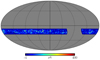 |
Fig. 1. Illustrative example of a FLASK simulation at the lowest redshift bin (0.127 < z < 0.138), convolved with a Gaussian beam of θFWHM = 40 arcmin, after selecting the sky region (apodized mask) considered in all the analyses. The color indicates the brightness temperature in μK. The Mollweide projection corresponds to celestial coordinates. |
We also accounted for the angular smoothing effect introduced by the BINGO beam, with θFWHM = 40 arcmin, which we approximated by a Gaussian of the same width for all the frequency bins. Each simulated sky map was convolved with such a Gaussian beam before thermal noise was added. In addition, we investigated the impact of θFWHM scaled with the frequency ν according to θFWHM(ν) = θFWHM(ν0) × ν0/ν, where ν0 = 1120 MHz and θFWHM(ν0) = 40 arcmin (Bigot-Sazy et al. 2015). Although in both cases we approximated the BINGO beam by a Gaussian, there will be contribution from structures such as the side lobes, discussed in the companion papers Wuensche et al. (2022) and Abdalla et al. (2022b), as well as the possible coupling of the horns, which is still to be investigated.
4.2. Foreground cleaning process
One of the main challenges of 21 cm IM observations is the efficient subtraction of the foreground contamination, whose amplitude can be up to 104 larger than the HI signal. Even when an efficient cleaning technique is employed, a residual contamination is expected to remain in the observations, and therefore it is important to evaluate their impact on the cosmological analyses. In this work, we used the GNILC method (Remazeilles et al. 2011), a nonparametric component separation technique, to perform the foreground cleaning process. This method has been tested in previous work and showed an excellent performance when applied to 21 cm IM observations (Olivari et al. 2016) and, more specifically, to the BINGO-simulated data (see Liccardo et al. 2022; Fornazier et al. 2022; Mericia et al. 2022).
The temperature signal, x(p), represented by a vector of dimension nch (where nch is the number of BINGO channels) for each sky pixel p, can be modeled as
 (18)
(18)
where s(p) is the 21 cm signal, n(p) is the instrumental noise, and f(p) is the total foreground signal. All contributions to x(p) have the same dimension nch. To distinguish foreground emission from 21 cm signals, GNILC exploits the fact that foreground emissions are highly correlated between frequencies channels and thus effectively rely on a few independent spectral degrees of freedom, while the 21 cm signal, probing shells at different redshifts, is only weakly correlated between frequency bands. Using a prior (theoretical template) of the 21 cm and thermal noise power spectra, GNILC evaluates the effective dimension of the foreground subspace locally in pixel and harmonic space, as identified by a principal component analysis of empirical channel data covariance matrices, computed on a redundant basis (a tight frame) of a type of wavelets on the sphere (called “needlets”). With this approach, GNILC does not use any prior information on the foreground components, except for the safe assumption that their emission between frequencies is strongly correlated. Then, GNILC projects the data x(p) out of the foreground subspace.
The 21 cm plus noise signal was then reconstructed for each wavelet scale by applying an ILC filter W to the data,  , in the subspace orthogonal to that of the foregrounds. The ILC filter was constructed in such a way as to preserve the 21 cm signal while filtering out the foreground contamination. The complete reconstructed 21 cm plus noise map at each frequency was finally obtained by adding the maps corresponding to each wavelet scale. A detailed discussion of the use of the GNILC method for 21 cm foreground cleaning can be found in Olivari et al. (2016) and Fornazier et al. (2022).
Finally, we emphasize that the reconstructed 21 cm maps contain a residual contribution from the foreground components along with the noise,
 (19)
(19)
where Wn and Wf are the residual noise and foreground contribution to the reconstructed 21 cm signal, respectively. In the case of simulations for which we know the exact input foreground contamination, as is the case here, we can then estimate its residual contribution over the recovered cosmological signal. Here, we used this facility to include a realistic foreground residual contribution to the simulations to evaluate its impact on the BAO fitting process, avoiding the need to apply GNILC to each one of them (see Sect. 6.3).
5. Method
This section summarizes the method we employed to extract the BAO information from BINGO-simulated HI maps. We describe (1) how the APS and ACF were measured from the simulated maps, (2) how the covariance matrices were calculated, and (3) the fitting method we used to estimate the α parameter from each of the simulations.
5.1. Clustering measurements
5.1.1. Angular power spectrum
The partial-sky coverage is a common situation for CMB and galaxy surveys, whether due to the observation strategy or to cuts of regions with strong foreground contamination. The APS computation in these cases is not as straightforward as it would be in full-sky analyses, where Cℓs are computed by expanding the radiation field in spherical harmonics and averaging the aℓm coefficients,
 (20)
(20)
The effect of a mask when calculating the aℓm coefficients over partial sky is to mix (or couple) different multipoles so that the estimated APS,  , can be written in terms of the true one, Cℓ, through
 (21)
(21)
where ℳℓℓ′ is the multipole mixing matrix, which depends on the mask geometry (Hivon et al. 2002).
Here we estimated the APS using the so-called pseudo-Cℓ formalism as implemented in the NaMaster code8 (Alonso et al. 2019). The mixing matrix was estimated analytically, according to the shape of the mask, and was used to obtain an unbiased estimate of Cℓ (for examples of application of this formalism and/or this code to different cases, see, e.g., Brown et al. 2005; Moura-Santos et al. 2016; Loureiro et al. 2019; Nicola et al. 2020; Anderson et al. 2022).
However, the loss of information due to the mask usually makes the mixing matrix ill-conditioned and, for this reason, singular, with no direct inversion. To deal with this, NaMaster allows the usage of bandbowers, calculating a binned and invertible version of ℳℓℓ′. Here, we considered a linear binning, calculating  at bins of width Δℓ, centered at ℓ. This procedure also helps making the corresponding covariance matrix more diagonal. Different Δℓ widths were tested so that we were able to find the more appropriate width that was to be used in the more realistic analyses, composing the fiducial configuration, defined when running the several robustness tests.
5.1.2. Angular correlation function
We measured the ACF from each of the simulations using the following equation (de Simoni et al. 2013):
 (22)
(22)
with δTp = Tb − ⟨Tb⟩, where Tb is the HI brightness temperature at each pixel p, and θ is the angular separation between pixels p and p′. The parameter wtp is associated with the observed sky region (mask information; Fig. 1), receiving value 1 when pixel i contains valid data and 0 when its area has not been observed or if it is located in the Galactic region and is removed from the analyses. The ω(θ), as given by Eq. (22), were calculated at equally spaced θ values, with a bin width Δθ, using the public code TreeCorr9 (Jarvis et al. 2004). In the same way as for the APS analyses, the best Δθ width for our fiducial configuration was defined after a few different values were tested.
5.2. Covariance matrix
We used N = 1500 FLASK and N = 500 N-body mock realizations to estimate the covariance matrices as
 (23)
(23)
where k and m indices ran over the different ℓ or θ bins, and i and j indicate the z-bin;  is the clustering measurement,
  or ωi(θ), and
  is the respective average over the simulations.
It is well known that the statistical noise in the covariance matrix estimated from simulations introduces a bias on its inverse, ![Mathematical equation: $ [\mathtt{C}^{ij}_{km}]^{-1} $](/articles/aa/full_html/2022/10/aa43158-22/aa43158-22-eq43.gif) , the precision matrix. The bias is mainly dependent on the number N of simulations used to construct
, the precision matrix. The bias is mainly dependent on the number N of simulations used to construct  and the number of entries Np of the data vectors X. However, as proposed by Hartlap et al. (2007) and as used, for example, in the analyses of Camacho et al. (2019), Ata et al. (2018), and Anderson et al. (2014), an unbiased version of the precision matrix can be obtained by rescaling it as
![Mathematical equation: $$ \begin{aligned}[\mathtt C ^{ij}_{km}]^{-1} \rightarrow \frac{N - N_{\rm p} - 2}{N - 1} [\mathtt C ^{ij}_{km}]^{-1}. \end{aligned} $$](/articles/aa/full_html/2022/10/aa43158-22/aa43158-22-eq45.gif) (24)
(24)
The rescaled version of the precision matrix was employed in all our analyses.
5.3. Parameter inference
The fit of the template models to the estimated clustering measurement goes through two (recursive) steps: one of them is to fit the nuisance parameters, B and Aq, appearing linearly in both template models, and the other step is to use the maximum likelihood estimator (MLE) to evaluate α, as described in Eqs. (15) and (16). Following Chan et al. (2018) and Camacho et al. (2019), we performed a least-square fit to find the best-fit Aq values, and, fixing them, we repeated the procedure to obtain the best-fit B value, in both cases by minimizing the χ2 defined as
![Mathematical equation: $$ \begin{aligned} \chi ^2(\lambda ) = \sum _{k,m} [X^i_k - x^i_k(\lambda )] \, [\mathtt C ^{ij}_{km}]^{-1} \, [X^j_m - x^j_m(\lambda )], \end{aligned} $$](/articles/aa/full_html/2022/10/aa43158-22/aa43158-22-eq46.gif) (25)
(25)
where λ = {α, B, Aq} and  is the template model for the ith z-bin and the kth ℓ/θ bin. We then maximized the likelihood function,
 (26)
(26)
now dependent on only one parameter, since χ(λ) is reduced to χ(α), allowing us to estimate the best-fit α value (see also Anderson et al. 2014). In practice, this value was obtained through a grid search, so that the least-square fit of the nuisance parameters, Aq and B, was repeated for each α value we evaluated.
Taking advantage of a tomographic approach, we were able to combine redshift bins so that the significance of the BAO detection can increase. We fit one α parameter through a joint analysis applying the MLE over a set of Nz consecutive z-bins. In particular, we fit the nuisance parameters, B and Aq, to each z-bin individually, and, fixing their values, we find one best-fit α for each set of Nzz-bins.
The 1σ error for the α estimates, σα, is defined as the deviation from the maximum likelihood point, at  , by Δχ2 = 1. It is worth noting that this Δχ2 = 1 rule is valid in the case of a Gaussian likelihood, L(p), for only one parameter, in our case, p = α (see Chan et al. 2018, and references therein, for details). In principle, this can be employed in our analyses, as commonly seen in literature (e.g., Ata et al. 2018; Carter et al. 2018; Abbott et al. 2019, 2022), but we have to be careful with deviations from Gaussian distribution, which can lead to σα values that underestimate the error bars. In the next section, we discuss and evaluate the validity of this rule for each clustering statistic used here.
6. BAO fitting results
In this section we present our findings from analyzing FLASK and N-body mock realizations. We start with an ideal case, analyzing pure 21 cm simulations, only accounting for the BINGO sky coverage and fixed 40 arcmin beam (Sect. 6.1). The contribution of thermal noise and foreground residuals are then considered one at a time, so that we can investigate the impact of each one separately, as well as the impact of a redshift-dependent beam size (Sects. 6.2 and 6.3). We also present the results from an extensive (but not exhaustive) list of robustness tests evaluating several aspects of the method employed here to extract the BAO signal from BINGO-like simulations, using FLASK mocks as the cosmological signal (Sect. 6.4). These tests allow finding the most appropriate configuration (hereafter called fiducial configuration), optimizing the analysis. In particular, the fiducial configuration is defined by
-
(a)
Angular and multipole binning: Δθ = 0.5° and Δℓ = 10,
-
(b)
Aq parameters for Cℓ and ω(θ) templates: q = −1, 0, 1, 2 and q = 0, 1, 2, respectively.
The 500 N-body mocks were analyzed using only this fiducial configuration (Sect. 6.5).
The choice for the range of scales, θ, and ℓ intervals is also important. Because the BINGO coverage is limited to a declination strip of ∼15°, the Cℓ determination at the smallest multipoles (ℓ ≲ 15) is compromised. Then, applying the BAO fitting to the (high signal-to-noise ratio) mean Cℓ from the 1500 FLASK mocks, we chose ℓmin ≈ 32, for which α estimate is the least biased with the smallest σα error. In this way, the choice of the multipole range can also account for any artifact introduced by the mask geometry, which would be more evident in the mean clustering measurement. Details about the fitting procedure over the mean APS and ACF are presented in the next subsections.
For all the z-bins we considered the same minimum multipole, but the maximum multipole was chosen according to the multipole ranges at which the BAO wiggles are concentrated, which are more spread out over higher multipoles the higher the redshift (Fig. 2). In this sense, after a few tests over the mean Cℓ, we chose 141 ≲ ℓmax ≲ 401 for lower to higher redshifts, so that we used only the range containing the BAO wiggles, avoiding to increase the number of data points with multipoles that do not bring information about the BAO signal (see discussion in Sect. 5.2).
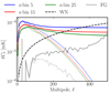 |
Fig. 2. Theoretical APS calculated for three of the 30 tomographic bins linearly spaced in frequency, whose average redshifts are |


A similar procedure was used to choose the θ range for the ACF analyses. Applying the BAO fitting pipeline over the mean ω(θ) measurements from the FLASK mocks, we chose for each z-bin the range of scales that was large enough to encompass slightly more than the full width of the BAO peak. Our choices for the θ ranges extend from 10.5° ⪅ θ ⪅ 21.0° for the smallest z-bin to 2.5° ⪅ θ ⪅ 8.0° for the highest z-bin.
The θ and ℓ ranges used for each z-bin in all our analyses are presented in Table 1. The large number of z-bins demanded a large number of tests to find the more appropriate angular and mutipole ranges for each estimator. We therefore only show our final choice in each case. We use the double tilde to refer to minimum and maximum θ and ℓ values because although these numbers are exact for the fiducial values of Δθ and Δℓ, they are slightly different when testing other binning schemes. For such cases, we chose the range of scales that was as close as possible to the fiducial configuration. This is shown in Table 1. All tests for choosing the best angular and multipole ranges were applied to the BINGO-like simulations because our goal was to optimize our analyses for future BINGO observations.
Maximum multipole, ℓmax, and minimum and maximum angular scales, θmin and θmax, in degrees considered for the template fitting over APS and ACF clustering estimates from each z-bin.
6.1. Fitting clustering measurements from 21 cm only simulations
Employing the fiducial configuration, we measured the BAO signal by jointly fitting three sets of Nz = 10 consecutive z-bins, the lower, intermediate, and higher z-bins (redshift ranges of Δz ≈ 0.09, 0.11, and 0.12 widths), estimating only one α parameter for each set. The advantage of a tomographic approach, combining different z-bins, is to improve the error bars and statistical significance of the measurements. The nuisance parameters, one parameter B and four (three) parameters Aq, were fit to the Cℓ (ω(θ)) estimated for each of the ten z-bins individually, so that for the fiducial configuration, we had a total of 10 × 5(4) = 50(40) nuisance parameters. The α fitting results obtained from analyzing the 21 cm only simulations (accounting for BINGO sky coverage and beam) are shown in the first part of Tables 2 and 3 for the ACF and APS estimators, respectively.
BAO fitting results for the ACF using 1500 FLASK mocks.
We started to test our BAO fitting pipeline over the high signal-to-noise ratio mean clustering measurements, that is, the mean Cℓ and ω(θ) from the 1500 FLASK mocks. Our aim in fitting a measurement with such a high signal-to-noise ratio is not only to help decide about angular and multipole ranges and their binning widths, Δℓ and Δθ, but also to be able to identify any possible systematic bias on α estimates. Hereafter, we use αm and  to denote the results of fitting the mean Cℓ or ω(θ), and α and σα the results for individual mocks. The fitting over the mean clustering measurement required dividing the original covariance matrix by the total number of simulations, but this scaling would not provide a realistic estimate of σα for one mock realization. Because likelihoods can be well approximated by Gaussians for high signal-to-noise ratio measurements of the BAO feature, we therefore followed Abbott et al. (2019) and divided the original covariance matrix by 10 to obtain the likelihood and fit the αm parameter. The corresponding 1σ uncertainty was calculated as described in the previous section and was then normalized to obtain
  . Using a different normalization factor, for example, 20 instead of 10, leads to similar error amplitude. The
  results are presented in the last column of Tables 2 and 3. Using the fiducial configuration to fit the mean clustering measurements from the 21 cm only simulations, we find a prediction of 24%, 10%, and 5% errors for the lower, intermediate, and higher z-bins, respectively. The same procedure was employed to all tests fitting the mean clustering measurements, namely, varying the fiducial configuration or/and including contaminant signals, whose results are shown in the last column of Tables 2–5 and are discussed in the next subsections. In general, αm estimates are consistent with unity, although they present a small bias, which in all the cases is well below the statistical uncertainty.
In addition, Tables 2–5 present the same summary statistics that were obtained applying the BAO fitting pipeline to each mock for each of the three redshift ranges. In particular, there we show the average shift parameter ⟨α⟩, the average error in α estimates ⟨σα⟩, and two measures of the dispersion of the α distribution, the symmetric error around ⟨α⟩ encompassing 68% of the mocks (less sensitive to the tails) σ68, and the common standard deviation of the distribution σstd, as well as the average ⟨χ2⟩ (and degrees of freedom, d.o.f.). All these quantities were calculated from the fraction Ns of the total 1500 mocks, which correspond to the mocks fulfilling our selection criteria, namely, those whose α ± σα interval are inside the range [0.6, 1.4] and that have  , where
  is obtained from fitting a non-BAO template model to the clustering estimates (see Sect. 6.6). This fraction Ns is also presented in the tables, as is the fraction Nd of the mock whose α estimate is inside the range [0.8, 1.2]. We consider these as the mocks with a BAO detection. Figures 3 and 4 show for ACF and APS the distribution of the α parameter, the σα error, and the χ2, estimated from the Ns fraction of the mocks, respectively; the blue curves show the 21 cm only results.
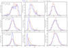 |
Fig. 3. Histogram distribution of the α parameter, σα error, and χ2 obtained by applying the BAO fitting pipeline to each of the FLASK simulations for the ACF estimator using the fiducial configuration. The rows from top to bottom show the results for each redshift range, the lower (1−10 z-bins), the intermediate (11−20 z-bins), and the higher redshifts (21−30 z-bins). The average redshift for each range is presented in the first panel of each row. In all the plots, the solid blue, dashed red, and dotted green lines show the distribution of the parameters resulting from analyzing the 21 cm only simulations (21 cm), the noisy 21 cm simulations (21 cm + WN), and the BINGO-like simulations (adding also the foreground residual; 21 cm + WN + FG), respectively. All these results correspond to the Ns fraction of the mocks. See Table 2. |
The detection criterion of having the full interval α ± σα inside the prior range [0.8, 1.2] (e.g., Ata et al. 2018; Chan et al. 2018) has commonly been employed in the literature. However, we can observe from these analyses that the distribution of the α parameter in general seems to be more Gaussian than what we find in our analyses (left panels in Figs. 3 and 4). A possible reason for this is the lower redshift we considered here, where the contribution from nonlinear effects is stronger. However, results from Villaescusa-Navarro et al. (2017), who investigated the BAO detection from 21 cm signal for the SKA case for the redshift range 0.35 < z < 3.05, also showed α distributions with clear deviations from a perfect Gaussian (but note the smaller number of simulations employed there, namely, 100). As pointed out by Chan et al. (2018) and Abbott et al. (2022), a natural consequence from having a (approximate) Gaussian distribution is a reasonable concordance among the three different error measurements, that is, ⟨σα⟩∼σ68 ∼ σstd. This is not our case, as can be seen from Tables 2 and 3 (as well as from Tables 4 and 5), indicating that ⟨σα⟩ is not meaningful or representative of the error in the α measurements for individual mock realizations (see also Figs. 3 and 4). Our results show that compared to ⟨σα⟩, the errors given by σ68 are overestimated by ∼18% to 33%, from the smallest to the highest z-bins when the ACF is used, but is underestimated by ∼50% for APS. Moreover, comparing the expected  obtained fitting the mean Cℓ and ω(θ) to the average ⟨σα⟩, we find a reasonable agreement for intermediate and higher z-bins, but not for the lower z-bins, in particular, for the ACF estimator. In addition, although σstd agrees better with σ68, we still find non-negligible differences among them, which confirms our α distributions as non-Gaussian (a larger σstd indicates non-Gaussian tails). These reasons motivated our choice of using the α values instead of α ± σα ranges, which belong to the interval [0.8, 1.2] as a criterion for a BAO detection (defining the Nd fraction), as well as our choice of using the 68% spread of the α distributions, σ68, as the representative error in our measurements.
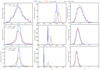 |
Fig. 4. Same as Fig. 4, but for the APS estimator. All distributions are again constructed from the corresponding Ns fraction of the mocks. See Table 3. |
BAO fitting results for the ACF using 500 N-body mocks.
Comparing the results obtained for the three redshift ranges, we confirm that the two clustering estimators perform better at higher redshifts, as expected. We recall that the lower the redshift, the larger the BAO angular scale, θBAO, which for the BINGO redshift range, 0.127 < z < 0.449, corresponds to 18° ≳θBAO ≳ 7° for the fiducial cosmology. This means that at the smallest redshifts, the θBAO is larger than the 15° stripe of the BINGO coverage, leading to worse statistics at these z-bins. Figure 5 compares APS and ACF results obtained from 21 cm only simulations (first row), showing the improvement in their performance for intermediate and higher redshifts, as well as a high correlation among their results. Comparing the performance from each of the clustering estimators, we found that they show different sensitivities to specific redshift ranges. Our results show that Cℓ measurements lead to smaller σ68 errors for intermediate and higher redshift ranges, namely, 20% and 25% smaller σ68 when compared to ω(θ). Furthermore, both Ns and Nd fractions of the mocks are larger for the APS at lower and intermediate redshifts, and comparable at higher redshifts. For the Nd fraction, the APS has ∼1.8 higher probability of detecting BAO at lower redshifts at 21 cm only mocks compared to the ACF.
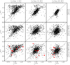 |
Fig. 5. Comparison of the α values estimated using the ACF and APS estimators (black dots). The columns from left to right show estimates from lower to higher redshift ranges, with average ⟨z⟩ = 0.172, ⟨z⟩ = 0.270, and ⟨z⟩ = 0.386. The first row shows results for the 21 cm only analyses, and the middle and bottom rows show results including white noise only and white noise + foreground residual, respectively. The red dots in the bottom row show α estimates from the reconstructed (foreground cleaned) maps. |
Finally, comparing the two estimators, we find in summary an apparently better performance of the APS over the ACF. This conclusion is mainly based on the following aspects of the ACF results: the slightly larger σ68 uncertainties at intermediate and higher redshifts; the quite larger bias on the average ⟨α⟩, especially at lower z-bins, corresponding to 0.95σ68; and the smaller Ns and Nd fractions at small and intermediate z-bins.
We also evaluated the z-bin width and the way in which the 30 z-bins were combined to estimate the shift parameter. First, the BAO fitting pipeline was applied to three ranges of redshift composed by Nz = 12, 10, 8 consecutive z-bins with δν = 9.33 MHz, so that α is estimated over three redshift ranges of same total width each (Δz ≈ 0.10). Then, we tested a tomographic binning of the BINGO frequency band into 30 z-bins linearly spaced in redshift (δz ≈ 0.01), instead of frequency, but still estimating α for three redshift ranges of Nz = 10 z-bins each (same total redshift width). We find that in general, both cases lead to results comparable to those from Tables 2 and 3, although each redshift range and clustering estimator has its own most advantageous configuration. In this sense, for simplicity, and because previous BINGO papers employ a redshift binning linear in frequency (Liccardo et al. 2022; Fornazier et al. 2022; Costa et al. 2022), we continued to use z-bins with δν = 9.33 MHz width and the BAO fitting process considering three sets of Nz = 10 z-bin for both estimators.
6.2. Impact of including instrumental noise
Taking all specifications summarized in Sect. 4.1.2 into account, we estimated the white noise level at each pixel in the BINGO region, σpix, considering the same resolution as was used to generate the 21 cm simulations, Nside = 256. From this σpix map, we generated as many realizations of the corresponding white noise map as necessary by multiplying it by random values defined by a Gaussian distribution of zero mean and unitary standard deviation. We added a different noise realization to each of the 1500 FLASK mocks and repeated the same process of calculating Cℓ and ω(θ) from each of them.
White noise adds a constant term Nℓ at all multipoles to the APS term, which for BINGO dominates the 21 cm signal as a function of redshift bin for ℓ ≥ 200 − 350 (Fig. 2). Then, we debiased the Cℓ from each noisy 21 cm simulation by subtracting the expected Nℓ amplitude, computed from the theoretical noise level. In contrast, white noise affects the ACF over all angular scales, so that this debiasing cannot be considered. However, because the ω(θ) was calculated by averaging over δTpδTp′ from all pairs of pixels p and p′ separated by θ (Eq. (16)), a natural consequence is a reduction of the noise.
Our results show that the presence of thermal noise increases the σ68 uncertainty by 19% and 90% for intermediate and higher z-bins when the ACF is used, while at lower z-bins, this error surprisingly diminishes by 14% (similarly to the respective bias on ⟨α⟩). The noise impact is more expressive for APS analyses, with an increase of 9%, 51%, and 122% in σ68 from lower to higher z-bins. However, although APS results are more affected by the noise, it still has a smaller σ68 uncertainty for higher z-bins, while for intermediate z-bins, the two estimators have comparable errors. The second row of Fig. 5 shows a comparison of the best-fit α from ω(θ) and Cℓ estimators. It is clearly much more spread due to the presence of noise. In addition, for both estimators, the Ns and Nd fractions decrease due to the presence of thermal noise, with the greatest impact over Ns, decreasing by 10% for the ACF estimator at lower z-bins. Again surprising, Nd increases by 6% for ACF at small z-bins after including noise. In addition, the number of simulations with a BAO detection decreases more strongly the higher the redshift. In summary, the presence of thermal noise has the main impact on higher z-bins, for which the BAO feature appears at smaller angular scales (spread to larger multipoles; Fig. 2), where noise starts to dominate.
6.3. Foreground residual contamination
The last step was to take residual foreground into account, as expected for BINGO. For this we added the most important foreground signals contributing to the BINGO frequency range along with the thermal noise (Sect. 4.1.2) to a 21 cm realization. Using the GNILC code, we performed component separation to reconstruct the noisy 21 cm signal as discussed in Sect. 4.2. Moreover, from Eq. (19), using the ILC filter and the known foreground contamination, we estimated the amplitude of the foreground residual in each z-bin, Wf. This process was repeated for ten different realizations of the 21 cm signal, each of them contaminated by a different realization of the thermal noise, but all with the same foreground signal contribution. These ten different estimates of the foreground residual were used to include the expected contaminant signal to each of the 1500 mock realizations (the BINGO-like simulations). The noise realizations are still different from one mock to another, while the foreground residual was repeated every ten mocks. This avoided the necessity of applying the (computationally expensive) component separation process to all the simulations.
Given the 1500 semi-realistic BINGO-like simulations, we calculated the Cℓ and ω(θ) from each of them and repeated the BAO fitting process using the fiducial configuration. We again debiased Cℓ by subtracting the expected Nℓ term. The results are shown in Tables 2 and 3, as well as in Figs. 3 and 4, for ACF and APS estimators, respectively. The last row of Fig. 5 also shows how the foreground residual can affect the concordance among the two estimators. In general, this contamination has a less significant impact, with negligible changes in the ⟨σα⟩, σ68, and σstd uncertainties compared to a case including noise (similar conclusions were drawn by Villaescusa-Navarro et al. 2017). Still, both Ns and Nd fractions decrease, especially at higher z-bins using ACF, and another ∼10% of the 1500 mocks no longer satisfy the selection and detection criteria. We note also that for all the redshift ranges, the best-fit αm from the mean ACF shows a slight shift to values lower than those found when only noise was included. Because this shift persists at some redshift ranges when the fiducial configuration was changed (Table 2) and also when the N-body mocks were used (Table 4), this suggests that the foreground residual might cause this systematic bias. For the APS, on the other hand, the results do not lead to the same conclusion. In any case, even though this shift is observed from ω(θ) results after the foreground residual contribution is included, it is quite small with respect to the error estimates, that is, small enough to be of no concern.
In order to evaluate the validity of including the expected foreground residual to the mocks, instead of applying the GNILC code to each of them, we added the BAO fitting results from the ten reconstructed maps to the last row of Fig. 5. The red dots appear to agree well with the black dots. The middle and last panels do not show all ten red dots because not all the reconstructed maps provided best-fit α values in the range [0.6, 1.4] for (at least) one of the estimators.
Additionally, we tested the impact of a frequency-dependent beam size, with the BINGO θFWHM taking values from ∼35′ to ∼45′ from low to high z-bins. In this case, the component separation was applied after the resolution of each frequency map (21 cm, along with thermal noise and foreground signals) was converted into the common θFWHM ∼ 45′, the largest beam size. The foreground residual for each z-bin was estimated as before. It was added to a realization after each frequency map, containing the 21 cm signal (FLASK mocks), convolved with the corresponding beam size, and the thermal noise, was converted into the common θFWHM. The BAO fitting results from this set of 1500 mock realizations are presented in the last part of Tables 2 and 3. These results show that for the two clustering estimators, a frequency-dependent beam size has a negligible impact on the BAO analyses for lower and intermediate redshift ranges. At higher z-bins, the bias on ⟨α⟩ for ω(θ) and Cℓ is slightly larger, but still quite smaller than the error estimates, and in addition, the Ns and Nd fractions for Cℓ and ω(θ) slightly decrease and increase, respectively. We find that the foreground residuals have a larger amplitude in the higher z-bins than when the beam size is fixed (Fig. 2), which mainly contributes at larger multipoles (a deeper investigation of the impact of the frequency-dependent beam size in the foreground cleaning is necessary, but beyond the scope of this paper and will be considered in future work). Still, even with a larger contribution, the foreground residual does not seem to have a significant impact on BAO results. This allows us to keep the previous conclusions.
6.4. Robustness tests
Here we test the aspects of the fiducial configuration, that is, we consider variations of (a) the angular (Δθ) and multipole (Δℓ) binning and (b) the q index in the templates, Eqs. (15) and (16). These robustness tests were performed over the BINGO-like simulations because they are the closest to what BINGO will observe. We varied only one aspect of the fiducial configuration at a time. This aspect is listed in the first column of Tables 2 and 3, where the results of all robustness tests are summarized.
From testing the Δθ width, Table 2 shows that the different binning leads to small changes at distinct statistics. The most discrepant result concerns the larger bias on αm obtained from the mean ω(θ) at all the redshift ranges for Δθ = 0.25°. Moreover, although Δθ = 0.40° shows slightly better results for some statistics, for example, larger Ns and Nd fractions at some redshift ranges, we find a smaller bias on ⟨α⟩ at higher z-bins for Δθ = 0.50°. In this sense, and in order to have a more diagonal covariance matrix, we chose to use Δθ = 0.50° as the fiducial configuration. Similar conclusions can be drawn from the tests on the ω(θ) template, showing that some choices of q can help to improve different statistics. However, by comparing all template tests, we note the large reduced ⟨χ2⟩ for all redshift ranges, using q = −2, 0, 1, and the large bias on ⟨α⟩ and αm for the ACF at small z-bins for q = 0, 1. In general, cases q = 0, 1, 2 and q = −1, 0, 1, 2 present the better results, especially in terms of the fraction Nd of mocks with BAO detection. The first case produces larger Ns and Nd for lower z-bins, while the second case provides larger fractions at higher z-bins. Given the smaller bias amplitude in ⟨α⟩ at higher z-bins, we chose q = 0, 1, 2 as part of the fiducial configuration.
Results from testing Δℓ width, presented in Table 3, show a good concordance between the different uncertainties from all three cases considered, but a clearly poorer performance for Δℓ = 20. While this larger bin width gives larger Ns and Nd fractions, it also introduces large bias on ⟨α⟩ and αm for most of the redshift ranges. When Δℓ = 10 and 15 are compared, the second case leads to slightly larger Ns and Nd fractions, but also to a larger bias on ⟨α⟩ and αm, as well as a larger ⟨χ2⟩, for the lower z-bins. It is therefore more appropriate to use Δℓ = 10 as part of the fiducial configuration. Finally, testing the different templates to fit Cℓ measurements, we again searched for the one with the smallest bias and uncertainty, combined with the largest Ns and Nd. In this sense, q = 0, 1, 2 and q = −1, 0, 1, 2 have the best results, but the latter gives a larger fraction of the mocks with BAO detection, Nd, and also larger Ns. We therefore chose it as part of the fiducial configuration.
From all the robustness tests, considering each redshift range individually, we might conclude that each of them would require a slightly different configuration. However, for simplicity, we chose to use the same θ/ℓ binning and ω(θ)/Cℓ templates for all three redshift ranges, that is, the (a) and (b) aspects of the fiducial configuration, as discussed.
6.5. Tests of N-body mocks
An additional test of the BAO fitting pipeline was its application on the set of 500 N-body mocks, generated through a completely different method, as described in Sect. 4.1.1. We employed the fiducial configuration to analyze the 21 cm only simulations and the BINGO-like simulations, constructed using the N-body mocks. We used the same ten foreground residual maps as before and a fixed beam size θFWHM = 40 arcmin. The summary statistics from these analyses are presented in Tables 4 and 5 for ACF and APS, respectively.
From the 21 cm only analyses, we find small differences with respect to what is obtained from the FLASK mocks, more expressive for the APS estimator, especially the smaller amplitude of ⟨χ2⟩ and fractions Ns and Nd for all the redshift ranges. However, these differences can be partially explained by the number of available N-body mocks: one-third of the number of FLASK mocks. The smaller number of simulations implies, for example, a lower signal-to-noise ratio from the mean clustering measurements, providing a poorer fitting over them (note the slightly large bias on αm from small and intermediate z-bins for both estimators). Additionally, for the APS (ACF), the number of d.o.f., increases (decreases) with the redshift, making the covariance matrix and its inverse the more biased the higher (lower) the redshift, explaining the discrepancy in the ⟨χ2⟩ and the uncertainty estimates. In this sense, we can argue that the slight differences between other summary statistics from N-body and FLASK mocks seems to be of statistical origin, although we also need to take into account that the two types of mocks were generated following very different methods.
The impact of introducing noise and foreground residuals to the N-body mocks is very similar to that obtained using the FLASK mocks. The greater impact appears in intermediate and high z-bins for the same reasons as previously discussed (see Sects. 6.2 and 6.3).
6.6. Wiggle versus no-wiggle template fitting
In order to evaluate the goodness of fit of the ω(θ) and Cℓ templates to the corresponding measurements from each mock, we compared the minimum χ2, evaluated at the best-fit αbf value, to that obtained by using a no-BAO template,  . To do this, we constructed a template model for each estimator (the same Eqs. (15) and (16)) using Ctemp(ℓ) obtained by imposing Ptemp(k) = Pnw, instead of using the parameterization from Eq. (14). The square root of the difference among the two quantities,
  , given in term of number of σ, is commonly used to evaluate the statistical significance of the BAO signal detection (see, e.g., Villaescusa-Navarro et al. 2017; Camacho et al. 2019; Abbott et al. 2022). This means that the BAO model (baryon signature) is preferred by Δχ2 compared to a model without the BAO.
To evaluate the effective significance of our BAO detection over BINGO-like simulations, we considered the complete BINGO redshift range, fitting all the 30 z-bins together instead of three subsets of them. Because the number of d.o.f. increases significantly in this case, namely, 256 and 604 for ACF and APS, respectively, an unbiased estimate of the covariance matrix and its inverse requires a larger set of simulations, which directly influences the χ2 estimate (see the discussion in Sect. 6.5). To do this, we rotated the original 1500 FLASK mocks six times, similarly to the procedure used to enlarge the number of N-body mocks, as described in Sect. 4.1.1, achieving a total of 10 500 mocks. The clustering statistics measured from the 10 500 BINGO-like simulations were used to estimate the covariance matrix, while the Δχ2 quantity was calculated only for the 1500 original mocks. The distribution of  from the corresponding Ns ∼ 90% and 94% of the mocks for ACF and APS, with average significance of ⟨S⟩ = 1.48σ and 1.61σ, respectively, are presented in Fig. 6. From the Ns fraction of mocks, we find ∼14% and ∼24% of them with
  , for ACF and APS, respectively. Confirming the slightly better performance of the APS over the ACF estimator, the first seems to provide a BAO detection with a higher significance than the last. Moreover, although the
  distribution is shown only for the BINGO-like simulations, it is impacted by systematic effects similarly to other summary statistics. Compared to 21 cm only case,
  is significantly shifted to lower values due to the inclusion of thermal noise, while the contribution of foreground residual has a negligible impact.
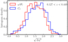 |
Fig. 6. Histogram distribution of the significance, |

7. Conclusions
The BAO feature measured from galaxy distribution is currently recognized as one of the most important cosmological probes. Its dependence on the evolution and the components of the Universe makes it a powerful tool for investigating the physical nature of dark energy. Since its first detection, the BAO scale has been measured using different matter tracers in several redshift ranges, and now the radio 21 cm IM experiments, such as BINGO, plan to provide a complementary route for studying the BAO.
We assessed the BINGO telescope potential in its phase 1 operation to detect the transversal BAO signal. To do this, we developed a template fitting pipeline with two clustering estimators, ω(θ) and Cℓ, to extract the BAO information from two different sets of simulations, FLASK and N-body mocks. Our analyses accounted for the BINGO sky coverage and beam effect and evaluated the impact of including thermal noise and foreground residual. The fitting procedure to measure the shift parameter, α, from the mocks was performed over three sets of consecutive z-bins using a maximum likelihood estimator. Most of our analyses were performed employing the fiducial configuration (aspects a and b defined in Sect. 6), optimized to be applied to all redshift ranges. Our main results are summarized below.
-
We found that both estimators perform better at higher redshifts, but show different sensitivities to specific redshift ranges. The bias amplitude in ⟨α⟩, the σ68 uncertainty, and the selection and detection fractions, Ns and Nd, suggest that the APS slightly outperforms the ACF estimator, although the ACF presents slightly smaller σ68 at lower z-bins. The APS also leads to a greater average significance, ⟨S⟩, than the ACF. This behavior is observed by analyzing 21 cm only simulations and remains after contaminant signals and redshift-dependent beam size are included (see Tables 2–5).
-
Accounting for the impact of including thermal noise and foreground residual one at a time, we found that the first affects the two clustering estimators more. It affects the results more significantly the higher the redshift. It enlarges the σ68 error significantly, in particular for the APS estimator, for which it reaches 122% in higher z-bins. The reason for this is that the BAO wiggles appear at higher multipoles (smaller angular scales) the higher the redshift. At these scales, the thermal noise starts to dominate. The inclusion of the foreground residual, on the other hand, does not seem to have a significant impact in our results.
-
Robustness tests of the fiducial configuration, considering different Δθ and Δℓ binning and alternative template models (q indexes), suggested that a more appropriate choice would be to select an optimal configuration for each of the three redshift ranges.
-
In the fiducial configuration, the BAO fitting pipeline applied to 500 N-body mocks (Tables 4 and 5) showed a few aspects that differed from those in the analysis of FLASK mocks. This is caused mainly by the smaller number of N-body mocks.
-
We also evaluated how preferred a BAO model is when compared to a fit of a non-BAO model, and found an average significance for the BAO detection of ∼1.48σ for ACF and ∼1.48σ for APS, combining all 30 z-bins. A fraction of 14% and 24% of the FLASK mocks for ACF and APS, respectively, provide a > 2σ BAO detection.
We emphasize that some aspects of the analysis presented here might benefit from the inclusion of more realistic choices of instrumental issues, such as the structure of the beam and instrumental effects such as 1/f noise and polarization leakage, or even aspects of the method that can be improved and deserve further study. These include a test of alternative component separation procedures, a different number of z-bins for the BAO fitting (see the results from the BINGO paper, Mericia et al. 2022), and a different fitting method from MLE.
Moreover, it is well known (Eisenstein et al. 2007b) that the nonlinear gravitational evolution of the Universe smears out the acoustic signature by inducing a damping and broadening on the BAO peak in addition to shifting its position so that the lower the redshift, the more difficult an accurate measurement of the BAO features. Because BINGO will survey a large volume of the Universe at relatively low redshifts, we also expect to improve our BAO fitting results, in particular at lower redshifts, by considering a reconstruction procedure (Obuljen et al. 2017).
In summary, we conclude that intermediate and higher redshift intervals are the most promising for measuring the BAO scale, with a probability of detection of more than ∼80% (∼70%) with the APS (ACF) estimator. These numbers are obtained using a fixed fiducial configuration and can be significantly improved by the choice of an optimal configuration for each redshift interval. Although we showed that systematic effects have a non-negligible impact on α estimates, our analyses of a semi-realistic scenario (BINGO-like mocks) confirmed that BINGO should be able to successfully detect the BAO signal at radio frequencies.
Acknowledgments
The BINGO project is supported by São Paulo Research Foundation (FAPESP) grant 2014/07885-0. C.P.N. would like to thank Edilson de Carvalho, Armando Bernui, Henrique Xavier, and Hugo Camacho for very enlightening and useful discussions. C.P.N. also acknowledges FAPESP for financial support through grant 2019/06040-0. J.Z. acknowledges support from the Ministry of Science and Technology of China (grant Nos. 2020SKA0110102). R.G.L. thanks CAPES (process 88881.162206/2017-01) and the Alexander von Humboldt Foundation for the financial support. L.S. is supported by the National Key R&D Program of China (2020YFC2201600). A.A.C. acknowledges financial support from the National Natural Science Foundation of China (grant 12175192). L.B., F.A.B, A.R.Q., and M.V.S. acknowledge PRONEX/CNPq/FAPESQ-PB (Grant no. 165/2018). E.F.: The Kavli IPMU is supported by World Premier International Research Center Initiative (WPI), MEXT, Japan. We thank an anonymous referee for her/his very insightful comments. This research made use of astropy (Astropy Collaboration 2018), healpy (Zonca et al. 2019), numpy (Van Der Walt et al. 2011), scipy (Virtanen et al. 2020) and matplotlib (Hunter 2007).
References
- Abbott, T., Abdalla, F., Alarcon, A., et al. 2019, MNRAS, 483, 4866 [NASA ADS] [CrossRef] [Google Scholar]
- Abbott, T., Aguena, M., Allam, S., et al. 2022, Phys. Rev. D, 105, 043512 [CrossRef] [Google Scholar]
- Abdalla, E., & Marins, A. 2020, Int. J. Mod. Phys. D, 29, 2030014 [NASA ADS] [CrossRef] [Google Scholar]
- Abdalla, E., Ferreira, E. G. M., Landim, R. G., et al. 2022a, A&A, 664, A14 [NASA ADS] [CrossRef] [EDP Sciences] [Google Scholar]
- Abdalla, F. B., Marins, A., Motta, P., et al. 2022b, A&A, 664, A16 [NASA ADS] [CrossRef] [EDP Sciences] [Google Scholar]
- Ade, P., Aghanim, N., Alves, M., et al. 2016, A&A, 594, A25 [NASA ADS] [CrossRef] [EDP Sciences] [Google Scholar]
- Alam, S., Ata, M., Bailey, S., et al. 2017, MNRAS, 470, 2617 [Google Scholar]
- Alam, S., Aubert, M., Avila, S., et al. 2021, Phys. Rev. D, 103, 083533 [NASA ADS] [CrossRef] [Google Scholar]
- Alonso, D., Bull, P., Ferreira, P. G., & Santos, M. G. 2015, MNRAS, 447, 400 [NASA ADS] [CrossRef] [Google Scholar]
- Alonso, D., Sanchez, J., & Slosar, A. 2019, MNRAS, 484, 4127 [Google Scholar]
- Anderson, L., Aubourg, E., Bailey, S., et al. 2012, MNRAS, 427, 3435 [Google Scholar]
- Anderson, L., Aubourg, E., Bailey, S., et al. 2014, MNRAS, 441, 24 [NASA ADS] [CrossRef] [Google Scholar]
- Anderson, C. J., Switzer, E. R., & Breysse, P. C. 2022, MNRAS, 514, 1169 [CrossRef] [Google Scholar]
- Astropy Collaboration (Price-Whelan, A. M., et al.) 2018, AJ, 156, 123 [Google Scholar]
- Ata, M., Baumgarten, F., Bautista, J., et al. 2018, MNRAS, 473, 4773 [NASA ADS] [CrossRef] [Google Scholar]
- Avila, F., Novaes, C. P., Bernui, A., & de Carvalho, E. 2018, JCAP, 2018, 041 [CrossRef] [Google Scholar]
- Avila, S., Vos-Ginés, B., Cunnington, S., et al. 2022, MNRAS, 510, 292 [Google Scholar]
- Bandura, K., Addison, G. E., Amiri, M., et al. 2014, Int. Soc. Opt. Photon., 9145, 914522 [Google Scholar]
- Battye, R., Browne, I., Dickinson, C., et al. 2013, MNRAS, 434, 1239 [NASA ADS] [CrossRef] [Google Scholar]
- Bigot-Sazy, M.-A., Dickinson, C., Battye, R. A., et al. 2015, MNRAS, 454, 3240 [NASA ADS] [CrossRef] [Google Scholar]
- Blas, D., Lesgourgues, J., & Tram, T. 2011, JCAP, 2011, 034 [Google Scholar]
- Brown, M. L., Castro, P., & Taylor, A. 2005, MNRAS, 360, 1262 [NASA ADS] [CrossRef] [Google Scholar]
- Camacho, H., Kokron, N., Andrade-Oliveira, F., et al. 2019, MNRAS, 487, 3870 [NASA ADS] [CrossRef] [Google Scholar]
- Carnero, A., Sánchez, E., Crocce, M., Cabré, A., & Gaztanaga, E. 2012, MNRAS, 419, 1689 [NASA ADS] [CrossRef] [Google Scholar]
- Carter, P., Beutler, F., Percival, W. J., et al. 2018, MNRAS, 481, 2371 [NASA ADS] [CrossRef] [Google Scholar]
- Carucci, I. P., Irfan, M. O., & Bobin, J. 2020, MNRAS, 499, 304 [NASA ADS] [CrossRef] [Google Scholar]
- Carvalho, G., Bernui, A., Benetti, M., Carvalho, J., & Alcaniz, J. 2016, Phys. Rev. D, 93, 023530 [NASA ADS] [CrossRef] [Google Scholar]
- Carvalho, G., Bernui, A., Benetti, M., et al. 2020, Astropart. Phys., 119, 102432 [NASA ADS] [CrossRef] [Google Scholar]
- Chan, K. C., Crocce, M., Ross, A., et al. 2018, MNRAS, 480, 3031 [NASA ADS] [CrossRef] [Google Scholar]
- Chang, T.-C., Pen, U.-L., Peterson, J. B., & McDonald, P. 2008, Phys. Rev. Lett., 100, 091303 [NASA ADS] [CrossRef] [Google Scholar]
- Chen, X. 2012, Int. J. Mod. Phys.: Conf. Ser., 12, 256 [CrossRef] [Google Scholar]
- Cole, S., Percival, W. J., Peacock, J. A., et al. 2005, MNRAS, 362, 505 [Google Scholar]
- Costa, A. A., Landim, R. G., Novaes, C. P., et al. 2022, A&A, 664, A20 [NASA ADS] [CrossRef] [EDP Sciences] [Google Scholar]
- Crichton, D., Aich, M., Amara, A., et al. 2022, J. Astron. Telesc. Instrum. Syst., 8, 011019 [NASA ADS] [CrossRef] [Google Scholar]
- Crocce, M., Cabré, A., & Gaztañaga, E. 2011, MNRAS, 414, 329 [NASA ADS] [CrossRef] [Google Scholar]
- Cunnington, S., Irfan, M. O., Carucci, I. P., Pourtsidou, A., & Bobin, J. 2021, MNRAS, 504, 208 [NASA ADS] [CrossRef] [Google Scholar]
- De Carvalho, E., Bernui, A., Carvalho, G., Novaes, C., & Xavier, H. 2018, JCAP, 2018, 064 [CrossRef] [Google Scholar]
- De Carvalho, E., Bernui, A., Xavier, H., & Novaes, C. 2020, MNRAS, 492, 4469 [NASA ADS] [CrossRef] [Google Scholar]
- de Carvalho, E., Bernui, A., Avila, F., Novaes, C., & Nogueira-Cavalcante, J. 2021, A&A, 649, A20 [NASA ADS] [CrossRef] [EDP Sciences] [Google Scholar]
- de Simoni, F., Sobreira, F., Carnero, A., et al. 2013, MNRAS, 435, 3017 [NASA ADS] [CrossRef] [Google Scholar]
- Delabrouille, J., Betoule, M., Melin, J.-B., et al. 2013, A&A, 553, A96 [NASA ADS] [CrossRef] [EDP Sciences] [Google Scholar]
- Dickinson, C., Davies, R., & Davis, R. 2003, MNRAS, 341, 369 [NASA ADS] [CrossRef] [Google Scholar]
- Dodelson, S. 2003, Modern Cosmology (Elsevier) [Google Scholar]
- Dunkley, J., Komatsu, E., Nolta, M., et al. 2009, ApJS, 180, 306 [NASA ADS] [CrossRef] [Google Scholar]
- Eisenstein, D. J., & Hu, W. 1998, ApJ, 496, 605 [Google Scholar]
- Eisenstein, D. J., Zehavi, I., Hogg, D. W., et al. 2005, ApJ, 633, 560 [Google Scholar]
- Eisenstein, D. J., Seo, H.-J., & White, M. 2007a, ApJ, 664, 660 [Google Scholar]
- Eisenstein, D. J., Seo, H.-J., Sirko, E., & Spergel, D. N. 2007b, ApJ, 664, 675 [NASA ADS] [CrossRef] [Google Scholar]
- Fornazier, K. S. F., Abdalla, F. B., Remazeilles, M., et al. 2022, A&A, 664, A18 [NASA ADS] [CrossRef] [EDP Sciences] [Google Scholar]
- Gorski, K. M., Hivon, E., Banday, A. J., et al. 2005, ApJ, 622, 759 [Google Scholar]
- Hall, A., Bonvin, C., & Challinor, A. 2013, Phys. Rev. D, 87, 064026 [NASA ADS] [CrossRef] [Google Scholar]
- Harper, S., Dickinson, C., Battye, R., et al. 2018, MNRAS, 478, 2416 [NASA ADS] [CrossRef] [Google Scholar]
- Hartlap, J., Simon, P., & Schneider, P. 2007, A&A, 464, 399 [NASA ADS] [CrossRef] [EDP Sciences] [Google Scholar]
- Hinton, S. R., Kazin, E., Davis, T. M., et al. 2016, MNRAS, 464, 4807 [Google Scholar]
- Hivon, E., Górski, K. M., Netterfield, C. B., et al. 2002, ApJ, 567, 2 [NASA ADS] [CrossRef] [Google Scholar]
- Hunter, J. D. 2007, Comput. Sci. Eng., 9, 90 [NASA ADS] [CrossRef] [Google Scholar]
- Jarvis, M., Bernstein, G., & Jain, B. 2004, MNRAS, 352, 338 [Google Scholar]
- Kennedy, F., & Bull, P. 2021, MNRAS, 506, 2638 [NASA ADS] [CrossRef] [Google Scholar]
- Kim, J., Park, C., L’Huillier, B., & Hong, S. E. 2015, J. Korean Astron. Soc., 48, 213 [Google Scholar]
- Lesgourgues, J. 2011, ArXiv e-prints [arXiv:1104.2932] [Google Scholar]
- Li, Y., Santos, M. G., Grainge, K., Harper, S., & Wang, J. 2021, MNRAS, 501, 4344 [NASA ADS] [CrossRef] [Google Scholar]
- Liccardo, V., de Mericia, E. J., Wuensche, C. A., et al. 2022, A&A, 664, A17 [NASA ADS] [CrossRef] [EDP Sciences] [Google Scholar]
- Loeb, A., & Wyithe, J. S. B. 2008, Phys. Rev. Lett., 100, 161301 [NASA ADS] [CrossRef] [Google Scholar]
- Loureiro, A., Moraes, B., Abdalla, F. B., et al. 2019, MNRAS, 485, 326 [NASA ADS] [CrossRef] [Google Scholar]
- McLeod, M., Balan, S. T., & Abdalla, F. B. 2017, MNRAS, 466, 3558 [NASA ADS] [CrossRef] [Google Scholar]
- Mericia, E. J., Santos, L., Wuensche, C. A., et al. 2022, A&A, submitted [arXiv:2204.08112] [Google Scholar]
- Miville-Deschênes, M.-A., Ysard, N., Lavabre, A., et al. 2008, A&A, 490, 1093 [NASA ADS] [CrossRef] [EDP Sciences] [Google Scholar]
- Moura-Santos, E., Carvalho, F., Penna-Lima, M., Novaes, C., & Wuensche, C. 2016, ApJ, 826, 121 [NASA ADS] [CrossRef] [Google Scholar]
- Nan, R., Li, D., Jin, C., et al. 2011, Int. J. Mod. Phys. D, 20, 989 [Google Scholar]
- Nicola, A., Alonso, D., Sánchez, J., et al. 2020, JCAP, 2020, 044 [Google Scholar]
- Obuljen, A., Villaescusa-Navarro, F., Castorina, E., & Viel, M. 2017, JCAP, 2017, 012 [CrossRef] [Google Scholar]
- Olivari, L., Remazeilles, M., & Dickinson, C. 2016, MNRAS, 456, 2749 [NASA ADS] [CrossRef] [Google Scholar]
- Peel, M. W., Wuensche, C. A., Abdalla, E., et al. 2019, J. Astron. Instrum., 8, 1940005 [NASA ADS] [CrossRef] [Google Scholar]
- Planck Collaboration VI. 2020, A&A, 641, A6 [NASA ADS] [CrossRef] [EDP Sciences] [Google Scholar]
- Remazeilles, M., Delabrouille, J., & Cardoso, J.-F. 2011, MNRAS, 418, 467 [Google Scholar]
- Remazeilles, M., Dickinson, C., Banday, A., Bigot-Sazy, M.-A., & Ghosh, T. 2015, MNRAS, 451, 4311 [NASA ADS] [CrossRef] [Google Scholar]
- Sánchez, E., Carnero, A., García-Bellido, J., et al. 2011, MNRAS, 411, 277 [CrossRef] [Google Scholar]
- Santos, M. G., Cluver, M., Hilton, M., et al. 2017, ArXiv e-prints [arXiv:1709.06099] [Google Scholar]
- Seehars, S., Paranjape, A., Witzemann, A., et al. 2016, JCAP, 2016, 001 [CrossRef] [Google Scholar]
- Seo, H.-J., & Eisenstein, D. J. 2007, ApJ, 665, 14 [Google Scholar]
- SKA Cosmology SWG (Bacon, D. J., et al.) 2020, PASA, 37, e007 [Google Scholar]
- Sobreira, F., de Simoni, F., Rosenfeld, R., et al. 2011, Phys. Rev. D, 84, 103001 [CrossRef] [Google Scholar]
- Tinker, J., Kravtsov, A. V., Klypin, A., et al. 2008, ApJ, 688, 709 [Google Scholar]
- Van Der Walt, S., Colbert, S. C., & Varoquaux, G. 2011, Comput. Sci. Eng., 13, 22 [Google Scholar]
- Villaescusa-Navarro, F., Alonso, D., & Viel, M. 2017, MNRAS, 466, 2736 [NASA ADS] [CrossRef] [Google Scholar]
- Virtanen, P., Gommers, R., Oliphant, T. E., et al. 2020, Nat. Meth., 17, 261 [Google Scholar]
- Weinberg, D. H., Mortonson, M. J., Eisenstein, D. J., et al. 2013, Phys. Rep., 530, 87 [Google Scholar]
- Wuensche, C. A., Villela, T., Abdalla, E., et al. 2022, A&A, 664, A15 [NASA ADS] [CrossRef] [EDP Sciences] [Google Scholar]
- Xavier, H. S., Abdalla, F. B., & Joachimi, B. 2016, MNRAS, 459, 3693 [NASA ADS] [CrossRef] [Google Scholar]
- Zhang, J., Motta, P., Novaes, C. P., et al. 2022, A&A, 664, A19 [NASA ADS] [CrossRef] [EDP Sciences] [Google Scholar]
- Zonca, A., Singer, L. P., Lenz, D., et al. 2019, J. Open Sour. Softw., 4, 1298 [NASA ADS] [CrossRef] [Google Scholar]
All Tables
Maximum multipole, ℓmax, and minimum and maximum angular scales, θmin and θmax, in degrees considered for the template fitting over APS and ACF clustering estimates from each z-bin.
All Figures
|
Fig. 1. Illustrative example of a FLASK simulation at the lowest redshift bin (0.127 < z < 0.138), convolved with a Gaussian beam of θFWHM = 40 arcmin, after selecting the sky region (apodized mask) considered in all the analyses. The color indicates the brightness temperature in μK. The Mollweide projection corresponds to celestial coordinates. |
| In the text | |
|
Fig. 2. Theoretical APS calculated for three of the 30 tomographic bins linearly spaced in frequency, whose average redshifts are |
| In the text | |
|
Fig. 3. Histogram distribution of the α parameter, σα error, and χ2 obtained by applying the BAO fitting pipeline to each of the FLASK simulations for the ACF estimator using the fiducial configuration. The rows from top to bottom show the results for each redshift range, the lower (1−10 z-bins), the intermediate (11−20 z-bins), and the higher redshifts (21−30 z-bins). The average redshift for each range is presented in the first panel of each row. In all the plots, the solid blue, dashed red, and dotted green lines show the distribution of the parameters resulting from analyzing the 21 cm only simulations (21 cm), the noisy 21 cm simulations (21 cm + WN), and the BINGO-like simulations (adding also the foreground residual; 21 cm + WN + FG), respectively. All these results correspond to the Ns fraction of the mocks. See Table 2. |
| In the text | |
|
Fig. 4. Same as Fig. 4, but for the APS estimator. All distributions are again constructed from the corresponding Ns fraction of the mocks. See Table 3. |
| In the text | |
|
Fig. 5. Comparison of the α values estimated using the ACF and APS estimators (black dots). The columns from left to right show estimates from lower to higher redshift ranges, with average ⟨z⟩ = 0.172, ⟨z⟩ = 0.270, and ⟨z⟩ = 0.386. The first row shows results for the 21 cm only analyses, and the middle and bottom rows show results including white noise only and white noise + foreground residual, respectively. The red dots in the bottom row show α estimates from the reconstructed (foreground cleaned) maps. |
| In the text | |
|
Fig. 6. Histogram distribution of the significance, |
| In the text | |
Current usage metrics show cumulative count of Article Views (full-text article views including HTML views, PDF and ePub downloads, according to the available data) and Abstracts Views on Vision4Press platform.
Data correspond to usage on the plateform after 2015. The current usage metrics is available 48-96 hours after online publication and is updated daily on week days.
Initial download of the metrics may take a while.