| Issue |
A&A
Volume 663, July 2022
|
|
|---|---|---|
| Article Number | A137 | |
| Number of page(s) | 26 | |
| Section | Stellar structure and evolution | |
| DOI | https://doi.org/10.1051/0004-6361/202243313 | |
| Published online | 21 July 2022 | |
Comprehensive analysis of southern eclipsing systems with pulsating components: The cases of HM Pup, V632 Sco, and TT Vel⋆
1
Institute for Astronomy, Astrophysics, Space Applications and Remote Sensing, National Observatory of Athens, Metaxa & Vas. Pavlou St., 15236 Penteli, Athens, Greece
e-mail: alliakos@noa.gr
2
School of Mathematics and Physics, The University of Queensland, Queensland 4072, Australia
3
Variable Stars South (VSS), Congarinni Observatory, Congarinni, NSW 2447, Australia
4
Astronomical Association of Queensland, St. Lucia, Queensland 4067, Australia
5
El Sauce Observatory, Coquimbo Province, Chile
6
ARC Centre of Excellence for All Sky Astrophysics in 3 Dimensions (ASTRO 3D), Australia
Received:
11
February
2022
Accepted:
20
April
2022
This work presents an extensive analysis of the properties of three southern semi-detached eclipsing binaries hosting a pulsating component, namely HM Pup, V632 Sco, and TT Vel. Systematic multi-filtered photometric observations were obtained using telescopes located in Australia and Chile mostly between 2018 and 2021. These observations were combined with data from the Transiting Exoplanet Survey Satellite (TESS) mission for a detailed analysis of pulsations. Spectral types and radial velocities were determined from spectra obtained with the Australian National University’s 2.3 m telescope and Wide Field Spectrograph. The data are modelled and the absolute parameters of all components are derived. The light curve residuals are further analysed using Fourier transformation techniques for the determination of the pulsation frequencies. Using theoretical models, the most probable modes of the principal oscillations are also identified. Eclipse-timing variation analysis is also carried out for all systems and the most likely mechanisms modulating the orbital period are proposed. The physical properties of these systems are compared with other similar cases and the locations of their components are plotted in the Mass-Radius (M−R) and Hertzsprung-Russell diagrams. Finally, the pulsational properties of the oscillating components are compared with currently known systems of this type within the orbital-pulsation period and log g-pulsation period diagrams. These systems are confirmed as oscillating eclipsing Algol-type systems (oEA stars), as the primary components are pulsating stars of δ Scuti type, with evidence of mass flow from the evolved secondary components present in their Na I D spectra.
Key words: binaries: eclipsing / stars: fundamental parameters / binaries: close / stars: oscillations / stars: variables: delta Scuti
Reduced WiFES spectra are only available at the CDS via anonymous ftp to cdsarc.u-strasbg.fr (130.79.128.5) or via http://cdsarc.u-strasbg.fr/viz-bin/cat/J/A+A/663/A137
© A. Liakos et al. 2022
 Open Access article, published by EDP Sciences, under the terms of the Creative Commons Attribution License (https://creativecommons.org/licenses/by/4.0), which permits unrestricted use, distribution, and reproduction in any medium, provided the original work is properly cited.
This article is published in open access under the Subscribe-to-Open model. Subscribe to A&A to support open access publication.
1. Introduction
A goal of asteroseismology is to improve the physics of stellar structure and evolution models by requiring such models to fit observed oscillation frequencies and modes of δ Scuti stars (Antoci et al. 2014). The single pulsating stars of δ Scuti type exhibit radial and non-radial oscillation modes triggered mostly by the κ mechanism (c.f. Aerts et al. 2010; Balona et al. 2015). Their pulsations are, in general, relatively fast (20 min–8 h), and typically show multi-periodic behaviour. The masses of these stars range between 1.5–2.5 M⊙ (Aerts et al. 2010), their temperatures between 6100–9800 K (A-F spectral classes), and their luminosity classes between III-V. They are located inside the classical instability strip and share a border in the colour-magnitude diagram (i.e. red edge of the classical instability strip) with the γ Doradus pulsating stars, which oscillate in lower frequencies up to 4 cycle d−1 (Handler 1999). In an analysis of 750 A-F type stars, observed by the Kepler mission (Borucki et al. 2010; Koch et al. 2010), Uytterhoeven et al. (2011) discovered that 63% are of δ Scuti or γ Doradus type or present a hybrid behaviour. The latter result regarding the hybrid nature of these stars is an open question to date.
The eclipsing binaries (EBs) are the ultimate astrophysical tools for determining the absolute parameters of stellar components. Their light curves (LCs) provide information about the luminosity and radius ratio of their components, as well as the orbital period, eccentricity, and inclination of the system. The radial velocities (RVs) of both components are required for calculating the mass ratio of the system. That is extremely critical for modelling eclipsing systems accurately, compared to models using only photometric data (i.e. degeneracy of solutions). Thus, combining photometry and spectroscopy of the EBs and using Kepler’s third law, we are able to calculate stellar physical parameters with a high accuracy. However, although the aforementioned methods concern the current status of an EB, using past eclipse timings and by applying the eclipse timing variation (ETV) method (also called as ‘O−C analysis’), it is feasible to identify short-, mid-, or long-term orbital period changes (such as cyclic or secular). These changes can be attributed to standard orbital period (Porb) modulation mechanisms, such as mass transfer, mass loss, additional components orbiting the EB, or even magnetic braking. Semi-detached Algol-type EBs have cool secondary stars that have filled their inner critical Lagrangian surface and are transferring mass to the hotter star, which was originally the less massive component. Emission in the Hα spectra of these systems has provided evidence of the mass flow and presence of circumstellar gas (Richards & Albright 1999). In systems where the cool component is very faint, Hα emission would only be detected during primary eclipses if the secondary component was larger than the hotter star. However, the Na I D lines of late K stars are relatively much stronger than those of their hot companions, thus they can reveal the presence of circumstellar gas at quadrature orbital phases, especially if the systemic velocity is large (Moriarty et al. 2019).
The high accuracy (order of 10−4 mag) and the continuity in time of the photometric data of Kepler (Koch et al. 2010; Borucki et al. 2010), K2 (Howell et al. 2014), and the Transiting Exoplanet Survey Satellite (TESS; Ricker et al. 2009, 2015) missions provide the means for detailed studies of stellar oscillations, especially in the case they are combined with multi-band photometry and high-resolution spectroscopy. The time resolutions for the data of these missions vary from 2 up to 30 min and they are quite useful for the determination of short-period frequencies, such as those met in δ Scuti stars. Given their accuracy, they also provide the opportunity to detect low-amplitude pulsations of the order of a few μmag (c.f. Murphy et al. 2013; Bowman & Kurtz 2018; Liakos 2020b; Kurtz et al. 2020; Liakos & Niarchos 2020; Kim et al. 2021). Moreover, these missions provide long time coverage (sometimes of the order of years) which is very useful for the calculation of many minima timings of EBs, which in turn, allows for a better study of their orbital period changes.
Eclipsing binary systems in which one component is a pulsating star are especially important in modern astrophysics as they provide the means to calculate the absolute properties of the pulsating star. The latter is quite significant and allows for the checking of stellar evolution theory and for the asteroseismology as well. Moreover, EBs hosting oscillating components and exhibiting mass transfer are very important in the field of asteroseismology as they show a different pulsational behaviour in terms of initiation, preservation, and evolution in comparison with those that are members of detached systems or are single stars (Liakos & Niarchos 2017; Liakos 2017; Mkrtichian et al. 2018b; Bowman et al. 2019). EBs of the Algol type, designated as oscillating eclipsing Algol (oEA) systems (Mkrtichian et al. 2002), contain an active cool G-K giant or subgiant star that transfers mass to a hot (A-F type) mass-accreting primary star of the δ Scuti type.
Currently, more than 330 binary systems with a δ Scuti component are known (Liakos & Niarchos 2017; Liakos 2018, 2020a, and personal collection from literature from 2020 and later – available online1). However, only 233 of these systems are EBs, while only 48 of these 233 are also double-line spectroscopic binaries (SB2), that is they can provide accurate absolute stellar properties. From these 48 EB+SB2 systems, only 21 are oEA stars, while the rest are in detached configurations. The aforementioned numbers indicate the difficulty and the importance in determining the absolute properties of pulsating stars in EBs.
This work is a continuation of the detailed study on individual oEA stars with a δ Scuti component (see also Liakos et al. 2012; Liakos & Niarchos 2013; Soydugan et al. 2013; Liakos & Cagaš 2014; Liakos 2017, 2018; Ulaş et al. 2020) and the first paper of a series dedicated to southern systems. We report analyses of three EBs that were apparently single-lined: HM Puppis, V632 Scorpii, and TT Velorum. These systems are previously known EBs exhibiting pulsations (Moriarty et al. 2013; Streamer et al. 2016; Mkrtichian et al. 2018a, respectively), but there is no detailed study for any of them nor any classification for their Roche geometry based on models to date. Therefore, this work significantly enriches the sample of oEAs with well-determined absolute stellar properties by ∼14% and the total number of known oEAs by ∼2.4%. For the selected systems, multi-band ground-based and space-borne photometric and low- and high-resolution spectroscopic data (see Sect. 2) have been collected in order to: (a) perform a detailed modelling (Sect. 3); (b) calculate the stellar parameters with high accuracy (Sect. 3); (c) perform ETV analysis for the determination of the most possible orbital period modulating mechanisms (Sect. 4); (d) detect the most powerful pulsation frequencies (Sect. 5); and (e) estimate the oscillation modes (Sect. 5). The properties of the systems as well as the pulsation properties of their oscillating stars are compared with others of a similar type (Sect. 6). Finally, a summary and conclusions are given in Sect. 7. In all tables of the present study, the errors of the parameters are given in parentheses alongside values and they correspond to the last digit(s).
2. Observations, data reduction, and analysis
In this study, three different data sources are used: (a) ground-based multi-band photometric time series; (b) TESS data obtained with long- (30 min), mid- (10 min), and short-cadence (2 min) modes; and (c) high and low resolution spectroscopic data for the calculation of RVs and spectral type determination.
2.1. Ground-based photometry
The ground-based data were obtained from three different observatories located at the southern hemisphere. Small-sized telescopes in Australia and Chile, equipped with CCD cameras and photometric filters, were employed for the observations. The majority of the data were collected between 2018 and 2021; however, for one system, data from 2013 and 2014 were also used in our study. The detailed log of observations is given in Table 1. It should be noted, that in one night more than one filter might have been used. After the completion of the LC of the EB, the B filter observations continued around the quadratures of the systems for a longer time coverage of the pulsations.
Ground-based photometric log of observations.
The data reduction was carried out with various photometric packages such as MaximDL (Diffraction Limited 2012) and AstroImageJ (Collins et al. 2017), using the differential aperture photometry technique. The magnitude calibration of the variables was based on the respective apparent magnitudes of the comparison stars taken from the AAVSO Photometric All-Sky Survey (APASS) DR9 (Henden et al. 2015) and the differential magnitude (for details see Moriarty et al. 2019). The phase-folded LCs of the systems are given in Sect. 3.
2.2. TESS photometry
The TESS data were downloaded from the Mikulski Archive for Space Telescopes (MAST2) archive. The log of observations for each system is given in Table 2, where the following are listed: the BJD of the beginning, the number of continuous days of observations, the sector (Sr) of TESS, the time resolution (Res.), and the number of points of each data set.
TESS log of observations.
For all systems, the Pre-search Data Conditioning Simple Aperture Photometry (PDCSAP) flux, which typically is corrected for long-term trends caused by instrumental effects, was used when available. However, in the data sets where the PDC pipeline produced distorted LCs, the SAP flux values were used instead. The magnitudes of the systems (assumed as the maximum brightness values) were taken from the TESS Input Catalog v8.0 (Stassun et al. 2019) and were used for the flux-to-magnitude conversion (Table 2).
For HM Pup, there are five data sets, two in long- and three in mid-cadence modes. For the latter ones (i.e. data sets of sectors 33–35), although PDCSAP flux values are available, they present obvious distortions, and therefore the SAP fluxes were used. V632 Sco was observed in long- and short-cadence modes. For the long-cadence data set, only the SAP flux is given, while the PDCSAP flux values are available for the short-cadence set. The time-series data sets for TT Vel were made in long- and mid-cadence modes. The PDCSAP flux was available, but as in the case of HM Pup, there are several distortions, thus, the SAP flux values were again used. Samples of the TESS LCs for all systems are plotted in Fig. 1, while the folded data in the orbital period are given in Fig. 10.
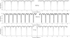 |
Fig. 1. TESS LCs that cover approximately 26 days of continuous monitoring. The rest of the data are not shown for scaling reasons. The time resolution of the data sets is 10, 2, and 10 min for HM Pup (top), V632 Sco (middle), and TT Vel (bottom), respectively. |
2.3. Spectroscopy
Spectra were observed with the wide field spectrograph (WiFeS) mounted at the Nasmyth focal position of the Australian National University’s 2.3 m telescope at Siding Spring Observatory, Australia (Dopita et al. 2007, 2010). The spectrograph is equipped with two Fairchild Imaging CCDs with a resolution of 4096 × 4096 pixels and a pixel scale of 0.5 arcsec. The 560 nm dichroic beam splitter was used. The detailed spectroscopic log of observations is given in Table 3. Readers can refer to Moriarty et al. (2019) for details on the procedures used to determine RVs and spectral types. In general, for RV determinations, sets of three or four spectra were observed at each phase with the B7000 grating, together with a spectrum of the Ne-Ar arc lamp before and after each set or closely grouped sets. Exposure times with the B7000 grating were long enough to allow for the detection of the faint secondary stars’ metal lines with the broadening function in RAVESPAN (Pilecki et al. 2017). On several occasions, at the same time as long exposure times were used with the B7000 grating, shorter exposure times were used with the R7000 grating to enhance the separation of Na I D lines of the primary stars from the lines due to circumbinary gas. As HM Pup is a totally eclipsing system, spectra of its secondary component can be observed during the 42 minute period of totality. We observed it twice with the B3000 grating for spectral classification and with the R7000 grating to seek evidence of chromospherical activity and mass flow.
Spectroscopic log of observations.
2.3.1. Spectral classification
Spectra for classification were observed with the low-resolution B3000 grating (708 lines mm−1, R = 3000). Its wavelength range of 3200–5900 Å includes the Balmer lines from Hβ-Hη, and the important Ca I K line (the Ca II H line is blended with Hϵ in the spectra of the A- and F-type stars in the systems studied here). The spectra of the primary components of HM Pup, V632 Sco, and TT Vel were observed during the secondary eclipse (phase 0.5) with short exposures to exclude an interference by their faint secondary components. The secondary component of HM Pup was observed at phase 0.0. All these spectra were corrected to heliocentric values by subtracting the systemic RVs of 58, −17, and 24 km s−1, respectively (see Table 4). Spectral types were determined using ‘XCLASS’ and ‘MKCLASS’ programmes (Gray & Corbally 2014). XCLASS provides a direct comparison of the target spectrum with reference spectra from the MKCLASS3 libraries, which encompass integer spectral temperature types from O6 to M5, and a wide range of luminosity types between V and Ia. The target spectra were normalised to unity at 4503 Å to match the library spectra.
Modelling and physical parameter results.
We classified the spectra initially by visual comparisons with selected reference spectra across the wavelength range of 3800–4600 Å. The best fits of the primary stars were: A6V for HM Pup, F2V for V632 Sco, and A8V for TT Vel. We classified the HM Pup secondary star as K8IV/III. The spectra were rectified to deliver a linear continuum baseline using the ‘Autorectify’ function in the XMK25 display routine in XCLASS (Fig. 2). These were then compared with other reference spectra, including the examples provided in the work of Gray & Corbally (2009).
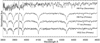 |
Fig. 2. Rectified spectra of the primary components of each system and the secondary component of HM Pup. |
2.3.2. Radial velocities
In general, for RV determinations, sets of three or four spectra were observed at each phase with the high-resolution B7000 grating (1530 lines mm−1, R = 7000) that provides a velocity resolution of 45 km s−1 and a wavelength range between 4180–5580 Å. Exposure times were long enough to allow for the detection of the metal lines of the faint secondary stars with the broadening function method in RAVESPAN software (Ruciński 1992, 2002; Pilecki et al. 2017). Spectra in the phase ranges shown in Table 3 were analysed. The optimum settings used for the three systems studied here were as follows. Spectra were normalised and analysed in the wavelength range 4355–4840 Å and 4880–5548 Å with the Balmer line masked. A template, with an effective temperature of 4000 K, a gravity coefficient set at 2.5, and a metallicity at 0.0, was selected from the synthetic spectra supplied with the RAVESPAN software (Coelho et al. 2005). A fourth-order polynomial was used with the resolution set at 2.0 km s−1 and a v range of 1.8. With these settings, the broadening function velocity peak of the secondary components was clearly evident (Fig. 3). The phased RV curves are plotted in Fig. 10, while the complete list of RV values is given in Table A.1.
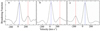 |
Fig. 3. Examples of broadening functions analyses on the spectra of (a) HM Pup at phase 0.25, (b) V632 Sco at phase 0.25, and (c) TT Vel at phase 0.75. Blue lines denote the RVs of the primary and red lines those of the secondary components. |
2.3.3. Chromospherical activity and gas streaming
Emission was observed in the centres of the Ca II H and K lines of the secondary component of HM Pup during the total primary eclipse. The emission peaks had a red shift of 58 km s−1 from the systemic velocity, indicating they were due to chromospherical activity and not circumbinary gas (Fig. 4). On the same nights, the Hα spectra had an emission peak with a blue shift of 120 km s−1 and the absorption line was broadened with a red shift from 33 to 110 km s−1 (Fig. 5). The Na I D lines of the secondary component on those nights were broadened towards red at velocities of 110–170 km s−1 (Fig. 5). Sky background flux values were subtracted from all the spectra in Figs. 4 and 5 since the exposures used were long. The sky background flux values in all spectra in Figs. 6 and 7 were 2–3 orders of magnitude lower than the stellar flux values; the difference was similar to that found for ST Cen and V775 Cen (Moriarty et al. 2019). Flux units are ergs cm−2 s−1 arcsec−2 Å−1.
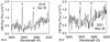 |
Fig. 4. Spectra of the HM Pup secondary star in the range 3900–4020 Å (with R = 3000) during totality on two occasions. The K and H emission peaks have a red shift of 58 km s−1. |
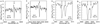 |
Fig. 5. Hα (a) and Na I D (b) spectra of the HM Pup secondary star observed at the same time as the Ca II spectra in Fig. 4, but with R = 7000. Arrows mark the calculated wavelength positions of the spectral line centres at the systemic velocity. |
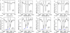 |
Fig. 6. Spectra of HM Pup Na I D lines at several orbital phases (Φ) with R = 7000. Downward arrows mark the calculated position of the line centres for the primary star that are the sum of the systemic and orbital velocities. Lines of circumstellar gas are marked with blue arrows. |
 |
Fig. 7. Spectra of Na I D lines at quadrature phases (R = 7000): (a, b) V632 Sco and (c, d) TT Vel. Downward arrows mark the calculated position of the line centres for primary components that are the sum of their orbital and systemic velocities. |
Broadening or splitting in the spectra of the sodium D doublet lines at different phases indicates evidence of gas streaming from the secondary components of Algol systems (see Moriarty et al. 2019). Circumstellar gas was particularly evident around HM Pup. The primary component’s sodium D line centres at phase 0.75 are red-shifted with a velocity of 103 km s−1 (the sum of the orbital and systemic velocities are of 45 and 58 km s−1, respectively). A clear separation of the sodium lines of the slower moving gas from the photospheric Na I D absorption lines of the receding primary star itself is clearly evident. Conversely, at phase 0.25, the sodium D lines of the approaching primary component were blended with the gas lines, which are evident as a broadening of the lines to the red (compare Figs. 6a–d with Figs. 6e–h).
In contrast to HM Pup, V632 Sco – with a negative systemic velocity – has sodium D line centres which are blue-shifted at phase 0.25 with a velocity of −69 km s−1; the sum of the orbital and systemic velocities are −52 and −17 km s−1, respectively. The narrow lines to the red side are evidence of circumstellar gas (Fig. 7a). At phase 0.75, the circumstellar gas lines are blended with those of the primary component, which are rotationally broadened (Fig. 7b). There was also evidence of circumbinary gas in the Na I D spectra of TT Vel, but its stellar and gas sodium lines were similarly blended at the resolution available to us (Figs. 7c,d). The sodium lines of the primary components of each system were strong in comparison to those of their secondary stars, which have low luminosities.
The Na I D absorption lines of circumstellar gas, seen against the continuum of the primary star of HM Pup, are distinctly separate from the Na I D lines of the stellar photosphere at phases between 0.6 and 0.9, as shown in Fig. 6. The full width at half maximum (FWHM) of the primary component’s absorption lines is 1.5 Å, based on the primary star’s rotational surface velocity; its velocity relative to the observer determines its central wavelength. Using these values, we were able to estimate the central position of the gas stream Na I D absorption lines at phases between 0.24 and 0.5 within the blended lines. This is illustrated in Fig. 8 for phase 0.28; the centre of the stellar Na I D2 line was determined to be 5890.24 Å. The shape of the blended absorption line indicates that the line centre of the gas stream is 5890.68 Å.
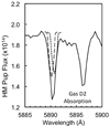 |
Fig. 8. Illustration of the method used to estimate the wavelength of the D2 line of the gas at phase 0.28. The primary star absorption line is long-dashed, and the gas is short-dashed. |
This method was used to estimate the observed velocities of the gas along the observer’s line of sight, and thence its velocity relative the primary star at a range of phases. These velocities (listed in Table B.1) were used to determine an approximate path for the gas streaming from the secondary star and around the primary (Fig. 9). The gas is shown as leaving the secondary star at the first Lagrangian point and orbiting the primary star (at least in part). The velocity and direction of the gas flow within this region are reflected in the observed gas velocities, particularly those between phases 0.24 and 0.32, where the gas appears to fall onto the primary star. A transient accretion cloud or annulus could be present, depending on the rate of mass loss from the secondary star. As discussed by Richards & Albright (1999), accretion disks do not develop around EBs with short orbital periods.
 |
Fig. 9. Estimated path of the HM Pup gas stream. The phases of the observations are marked around the periphery of the dashed circle, and the corresponding observed gas velocity and direction relative to the primary star are indicated inside the circle. The orbital direction and direction of rotation of the two stars are shown by the long-dashed and short-dashed arrows, respectively. The wavelengths and velocities were adjusted, for clarity, to remove the fixed systemic velocity of 58 km s−1. |
3. Light and radial velocity curve modelling and calculation of absolute parameters
The light and RV curves of the three systems were analysed with ‘PHOEBE’ v.0.29d software (Prša & Zwitter 2005), which uses the 2003 version of the Wilson-Devinney code (Wilson & Devinney 1971; Wilson 1979, 1990). Temperatures, T, of the components were given values derived from the spectral classification (see Sect. 2.3.1) and the spectral type-temperature correlation of Cox (2000). The temperatures of the primary components were kept fixed during the analysis, while those of the secondaries were adjusted. For all systems, the albedos, A, and gravity darkening coefficients, g, of the components were given values according to their spectral types (Ruciński 1969; von Zeipel 1924; Lucy 1967). As the maxima of the LCs are displaced towards the secondary minimum (typically between phases 0.25–0.45 and 0.55–0.75) as a result of reflection due to the heating of the secondary components’ atmospheres by the hot primary components, A2 was adjusted. The (linear) limb darkening coefficients, x, for the B, V, and I filters were taken from the tables of van Hamme (1993), while those for the TESS photometric system, xTESS, are from Claret (2018, Table 5 in that work). The dimensionless potentials Ω and the fractional luminosity of the primary component L1 were also adjusted during the modelling. The systemic RV, Vsys, the mass ratio, q, and the inclination of the system, i, were set as free parameters. As the three systems exhibit cyclic orbital period modulations (see Sect. 4) that could potentially be attributed to tertiary component(s), the third light parameter, l3, was tested initially, but it converged to a zero value in each case and, therefore, it was excluded from further modelling.
Intense magnetic dynamo activity is expected in close EBs with convective outer regions and rapid rotation rates locked to their orbital velocities (see Berdyugina 2005). The magnetic activity causes variability or asymmetry in LCs which could affect the modelling results. Several LC cycles for each system were obtained from the TESS data (see Table 2). We carefully examined them to determine the stability of the asymmetries in successive LCs, and then decided how to proceed with the model. There were 20 and 12 complete LCs of mid-cadence data for HM Pup and for TT Vel, respectively, which, although displaying some variability, were sufficiently stable for modelling over the time range of the observations. However, in the case of V632 Sco, there were 12 complete LCs of short-cadence data which show noticeable changes every few days. Therefore, for this system, we modelled three groups of four LCs folded into the Porb.
Given that the purpose of this work concerns mostly the asteroseismology of these systems, we excluded the long-cadence data of the systems from the modelling and kept only those with the best available time resolution. However, the long-cadence data were used for minima timing calculations (see Sect. 4). As with the TESS data, the ground-based observations obtained in different time periods show asymmetries that cannot be fitted easily in a unique phased LC. In order to avoid this in our study, we again modelled the LCs of each system separately, according to the asymmetries found. In particular, as V632 Sco is more active than the other two systems, in order to have complete LCs for the modelling, photometric observations in the V and I passbands over several years were combined. The examination of the LCs was carried out with great care, as the LC residuals are used later for frequency analysis. They must, therefore, be kept free of any proximity or stellar magnetic activity effects.
During the modelling process, all LCs from each passband were used initially with the RVs to derive the mean model of each system. Then, the values from the output of the mean model were used as initial inputs to model the individual phase-folded LCs (or groups of LCs) mostly by adjusting the spot parameters, namely the Co-latitude, longitude, radius, and temperature factor. Thus, the parameters of the final model of each system are the average of the respective parameters of each LC model, and their uncertainties are the standard deviations. This procedure gives more realistic uncertainty values in comparison with the direct errors derived from ‘PHOEBE’ (c.f. Liakos 2017, 2018). Three modes of LC analyses were tried: mode 2 (detached system), mode 4 (semi-detached system with the primary component filling its Roche lobe), and mode 5 (conventional semi-detached binary). Models for the three systems converged in mode 5. Therefore, all of them are semi-detached systems with their secondary components (less massive and cooler) filling their Roche lobes; thus, they are classical Algols (from an evolutionary point of view). The amplitudes K1 and K2 were calculated using sinusoidal fittings on the respective RVs. The (linear) ephemeris of each system, that is the orbital period, Porb, and a reference time of a primary minimum, T0, was based on the observed times of minima between 2012 and 2020 (see Sect. 4). The absolute parameters of the components were calculated based on the modelling results using the ‘AbsParEB’ software (Liakos 2015, mode 3). The upper and middle parts of Table 4 list the LCs’ and RVs’ modelling parameters, while the lower part of it provides the absolute parameters of the components. The fit on the LCs and RVs for all systems are given in Fig 10. The spots parameters for each system are given in Table C.1.
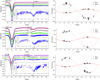 |
Fig. 10. Synthetic (solid lines) over observed (points) LCs (left plots) and RVs (right plots) for HM Pup (top panels), V632 Sco (middle panels), and TT Vel (bottom panels). Some LCs were vertically shifted for scaling reasons. The fit on the out-of-primary eclipse points of the B filter was re-scaled and plotted allowing for better viewing. |
4. Orbital period variation analyses
In order to determine whether orbital periods of the systems have changed, accurate eclipse times over a long period of time are necessary in order to apply an ETV analysis. For this, the first step was to gather the past times of minima from the literature and relevant minima databases and calculate new ones from our ground-based LCs as well as from the TESS data. Subsequently, these minima timings were used for the construction of the ETV plots and were fitted by various curves that correspond to different orbital period modulating physical mechanisms.
The times of minima of the systems observed at the Congarinni, El Sauce and Glen Aplin observatories were calculated in PERANSO4 from a seventh-order polynomial fit to the light curves spanning two hours on each side of the minima. Past times of minima were collected from the ‘O–C gateway5’, ‘TIDAK6’ (Ogloza et al. 2022, TIming DAtabase at Krakow; former O–C atlas; private communication with B. Zakrzewski), and the International Variable Star Index (VSX) databases7 and other literature sources containing times of minima. For eclipses observed in multiple filters in the same night, the average of the timings derived from each filter was used. All available TESS data sets (see Table 2) were used for minima timing derivations. Due to the huge amount of observations in each data set, the software ‘B-Minima’ v.1.2 (Nelson 2005) was used; it searches and calculates minima timings automatically in big files. The calculated times of minima are given in Table D.1.
The mass transfer and mass loss mechanisms that are expected to occur in semi-detached EBs were tested for the studied systems. Mass transfer stipulates secular changes of Porb, while the ETV points present a parabolic distribution, whose curvature indicates the direction of the mass transfer (i.e. upward means mass transfer from the less to more massive component). The parabolic coefficient C2 can be determined by fitting a parabola on the data points, and it is used to calculate the Porb change rate (Ṗ) using the following equation (c.f. Kalimeris et al. 1994):

In the case of conservative mass transfer, the mass transfer rate (Ṁtr) is calculated with the following equation (c.f. Kruszewski 1966; Hilditch 2001):
where M1 and M2 are the masses of the components of the EB.
Mass loss from EB systems can be due to stellar winds. This mechanism causes an increase in the orbital period, which is reflected as an upward parabolic distribution of the ETV points. The mass loss rate, Ṁloss, is computed according to the formula of Hilditch (2001):
Cyclic changes in the orbital period can be explained by either the Light-Time effect Irwin (1959, LITE) or with variations in magnetic cycles that could also modulate changes in eclipse timing due to the effect of star spots or with changes in the magnetic quadrupole moment in the secondary star (Applegate mechanism Applegate & Patterson 1987; Applegate 1992; Lanza et al. 1998; Hoffman et al. 2006; Rovithis-Livaniou et al. 2000; Lanza & Rodonò 2002). Applegate’s mechanism, however, is not likely to contribute significantly to period modulation in systems such as those in this study (Lanza 2006; Völschow et al. 2018). An alternative mechanism involving a persistent non-axisymmetric internal magnetic field in the active component (Lanza 2020) may explain the observed ETV. However, an in-depth examination of the cyclic modulations of the orbital periods of the systems are beyond the scope of this study.
Eclipse times were analysed with the LITE code of Zasche et al. (2009) that uses the method of statistical weights according to the method used for the observations of the eclipses. Statistical weights, w, were applied as follows: visually or photographically determined minima were assigned w = 1, and the photoelectric and CCD minima were assigned w = 10. This method works well when the minima timings are spread uniformly in time. For V632 Sco and TT Vel, most eclipse times were obtained after the year 2000. Moreover, there are a lot of minima timings from the TESS mission that cover only one or two years. In order to avoid over-weighting only one part of the ETV distribution, the TESS data were given w = 1 instead of ten. Using this method, the many data points gathered within a short time range do not drag the fitting functions on them. In addition, minima timings based on the data of the ASAS (Pojmanski 2002), ASAS-SN (Shappee et al. 2014), and Catalina (Drake et al. 2009) surveys (included in the TIDAK database) were given w = 1 due to their large uncertainties.
The code can fit one parabola and up to two LITE curves simultaneously. The initial ephemerides used for the ETV diagrams of the systems were taken from the ‘TIDAC’ and ‘O–C gateway’ databases. The ephemeris (T0-reference time of minimum and Porb), the period of the modulation P3, the amplitude of the ETV variation AETV, the argument of periastron ω3, the eccentricity e3, and the time of the periastron passage Tper of the additional body are the free parameters of each LITE fitting curve. Moreover, the parabolic coefficient C2 is also adjusted when a parabola is selected for the fit (for more details see Zasche et al. 2009). The selection of the final model is based on the Bayes information criterion (BIC).
Analyses of eclipse times of HM Pup did not show evidence of mass transfer, that is to say no secular changes were detected. However, one possible cyclic variation was found (Fig. 11). The results from a LITE curve fit are shown in Table 5. The proposed mass of the additional component would require a comparable large luminosity, but there was no evidence for that in our spectroscopic observations nor in the LC analysis. Therefore, other modulating mechanisms need to be tested to find an explanation for this cyclic change. Moreover, a second LITE curve was tested because the data points after 2000 show evidence of an additional cyclic change. However, this LITE curve was proven statistically insignificant based on the BIC and it was excluded.
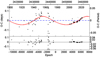 |
Fig. 11. Eclipse timing variations plot for HM Pup. Top panel: O–C points of the system fitted by a LITE curve (upper part) and the residuals (lower part) of the fit. For both panels, the bigger the symbol is, the bigger the statistical weight of the individual points. |
ETV analysis results.
For V632 Sco, there was only one published time of minimum before the year 2000, that is in 1939. A parabola was chosen to fit the data (Fig. 12, top panel), but the residuals show an additional cyclic distribution. Therefore, a LITE curve was also tested and is plotted in Fig. 12 (bottom panel). Results for several possible mechanisms are given in Table 5 and they were calculated using the ‘InPeVEB’ software (Liakos 2015). The upward curvature of the parabola is in good agreement with what would be expected for a conventional semi-detached configuration of this EB. It is a classical Algol system with mass transfer from the less to more massive component and a rate of ∼2.1 × 10⁻⁸ M⊙ yr−1. The third body hypothesis suggests a minimum mass of 0.66 M⊙ and a potential luminosity contribution of only about ∼1.8% in the system (following the formalism of Liakos et al. 2011). This contribution would not have been detectable in the analyses of LCs and RVs.
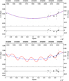 |
Fig. 12. Eclipse timing variations plots for V632 Sco. Top panel: O–C points of the system fitted by a parabola (upper part) and the residuals (lower part) of the fit. Bottom panel: same as previous panel, but with the fit of a parabolic and LITE curves. |
Most of the eclipse timings for TT Vel were carried out in the past two decades; after its discovery in 1913, only a few timings were reported in the late 1930s. In the ETV analysis, a parabola fitted the data (Fig. 13, top panel). The residuals indicated a periodic trend, to which a LITE curve was fitted (Fig. 13, bottom panel). The orbital period changes agree with a conservative mass transfer from the less to more massive component of the system with a rate of ∼4.9 × 10⁻⁸ M⊙ yr−1. The cyclic changes can be explained by the LITE that suggests a low mass component (M3,min ∼ 0.34 M⊙), whose light contribution is found less than 0.5%. Therefore, its absence from photometry and spectroscopy is plausible.
5. Pulsation analyses
The search for oscillation frequencies was carried out with the software PERIOD04 v.1.2 (Lenz & Breger 2005), which is based on classical Fourier analysis. Given that the typical frequency range of δ Scuti stars is 4–80 cycle d−1 (Breger 2000; Bowman & Kurtz 2018), yet as many of them exhibit slower modes (e.g., due to possible γ Doradus-δ Scuti hybrid nature and/or due to g-mode pulsations), the search was expanded to slower frequency regimes, that is 0–80 cycle d−1. For the analysis of the pulsations, only the best quality ground-based data and the TESS data with the best available time resolution were used. For this analysis, the binary model was subtracted from the observed LCs (see Sect. 3 for details) of each system and the Fourier method on the time-series residuals data was applied. Moreover, since the pulsation amplitudes are modified during the eclipses, and in order to keep a homogeneous data sample, only the out-of-eclipse data points were used. For the three systems, the data corresponding to phases 0.92–0.08 and 0.42–0.58 were excluded.
The S/N of the frequencies was calculated around the area of the signal (Balona 2014) with a spacing of 2 cycle d−1 and a box size of 2. A S/N = 4, suggested by the developers of the software (see also Breger et al. 1993), as the minimum value of a detected frequency to be considered as reliable was adopted. However, this threshold concerned only the ground-based data sets. For the TESS data, based on the conclusions of Baran et al. (2015), Baran & Koen (2021), and Bowman & Michielsen (2021), a S/N = 5 value was adopted. After the detection of a frequency, the software subtracts it from the observed points and searches for another in the new residuals’ data until the amplitude of the last frequency reaches the critical S/N.
Representative Fourier fittings on the data points of B filter (because the maximum amplitude of the pulsations is met in this pass band) and TESS (due to their high photometric accuracy) are given for all systems in Fig. 14. The respective periodograms are illustrated in Fig. 15, where the strongest detected frequencies are indicated. In Table 6 we list the properties of the data sets used in the frequency analysis. The independent pulsation frequencies are listed in Table 7. The complete lists of detected frequencies, also including the S/N and the most possible combination of each one, are given in Appendix E for each studied system.
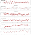 |
Fig. 14. Representative Fourier fit on the data of B filter and TESS. |
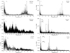 |
Fig. 15. Periodograms of B filter (left panels) and TESS data (right panels). Some of the detected strong frequencies are indicated. |
Properties of the data sets used for the frequency search.
Probable independent pulsation frequencies for each observed band.
The results from the spectral classification (Sect. 2.3.1) as well as the frequency regimes where the majority of the frequencies are detected (i.e. 0–4 and 10–40 cycle d−1; see Tables 7, E.1, E.3, and E.4) clearly suggest that the primaries of the studied systems are pulsating stars of δ Scuti type. The pulsations constant, Q, of the independent frequencies are calculated using the formula of Breger (2000):

where f is the frequency of the pulsation mode, while log g, Mbol, and Teff denote the standard quantities (see Table 4, bottom part). The density of the pulsating star, ρpul, is calculated with the pulsation constant - density relation:
where fdom is the frequency of the dominant pulsation mode. Alternatively, the ρpul can also be computed using the physical parameters of the stars directly (Table 4), that is  . For the oscillation mode identification, the theoretical MAD models for δ Scuti stars (Montalbán & Dupret 2007) in the FAMIAS software v.1.01 (Zima 2008) were used. Given that for all systems multi-colour photometry is available, FAMIAS uses the amplitude and the phase ratios in different filters for a given frequency to estimate the most likely l degrees based on the theoretical models’ grids. However, it should to be noted that these models are based on the absolute parameters (log g, M, and Teff) of the pulsators and they have been calculated for single δ Scuti stars. The pulsating stars of the studied systems have increased mass values due to the mass transfer (i.e. their Teff is low for their mass in comparison with main-sequence stars; see Cox 2000), hence, the results for the l degrees can be considered as only approximate.
The following subsections include comments on the analysis and results for each system, while a discussion regarding the real pulsation frequencies is also provided. The latter discussion for each system is based on the comparison between the detected frequencies in the different passbands of observations. The indices of the compared and discussed frequencies have, in addition to their increasing number, a filter designation in order to be checked more easily by the reader in Tables 7, E.1–E.4. It is quite common in EBs with pulsating components that the imperfect fit of the LCs produces artificial slow frequencies that are connected to instrumental and observational drifts. The time gaps between the ground-based observations may also produce alias frequencies (Breger 2000). Furthermore, searching for pulsations in light curves with removed eclipses also creates aliases at the orbital frequency and multiples thereof. Therefore, distinguishing the real independent frequencies from the possible artefacts is done using the data obtained in bluer passbands (i.e. B and V) as indicators for the low-amplitude frequencies (i.e. the pulsations show larger amplitudes in these bands) and the TESS data as an indicator for the slow frequencies (i.e. no time gaps and a higher photometric accuracy). All periodograms were checked for potential sidelobes due to the fast rotation of the pulsating stars (i.e. due to the tidal locking), but none of them showed such evidence. Finally, Table 8 includes the Q value and the most possible oscillation mode (l degrees) for the independent frequencies identified as real as well as the ρpul of each pulsating star.
Independent pulsation frequencies and MAD model results for the δ Scuti stars in each system.
5.1. HM Pup
For this system, B, V, I, and TESS data were used for the pulsations search. As listed in Table 6, many data points in B, V, and I filters were available; they have a very good time resolution (< 2 min) and cover a time span of more than 40 days. On the other hand, the available TESS data have a 10 min time resolution, but they cover ∼78 consecutive days. Moreover, and clearly by chance, the majority of the ground-based observations in the B and V filters and all the data of the I filter for this system were acquired during the TESS observations.
The independent frequencies 38.56 cycle d−1 and 36.42 cycle d−1, as can be seen in Table 7, are detected in all data sets, and therefore they are valid. The f8, V was identified as independent only in the V filter, while its value is very close to that of f13, B, f21, B, and f22, T (see Table E.1), thus it is probably not an independent frequency. The frequency f5, V was not detected in any of the other filters; therefore, it is probably an artefact. Finally, f1, B and f4, T concern a slow frequency of the order of 0.03 cycle d−1. Although its absence in the V and I filters is spurious, especially since it has the highest amplitude in B, we cannot neglect its presence in TESS data. Therefore, this frequency can be characterised as suspected-independent frequency. According to the MAD models, the most probable l degrees for the f2, B (=f1, V = f1, I = f1, T) and f3, B (=f2, V = f2, I = f2, T) are l = 2 and l = 1, respectively. The complete list of detected frequencies is given in Table E.1.
5.2. V632 Sco
For the pulsation analysis of V632 Sco, we used the short-cadence data set of TESS (see Table 2) and only the data set obtained from the Congarinni observatory (see Table 1), because it was obtained over a much shorter time period and has higher time resolution in comparison with that obtained from the Glen Aplin observatory. Eight nights of observations in the B filter within a time range of ∼57 d were available, only two in the V filter, and none in the I passband. The TESS data cover ∼28 d of continuous monitoring; therefore, the analysis relies mostly on them.
The frequency ∼23 cycle d−1 was detected in all data sets, and therefore it is considered as the dominant independent frequency. The second frequency detected both in B and TESS data is the f4, B (=f5, T), thus, we conclude that this is also an independent frequency. The frequency f1, B, which is found to be the strongest frequency, is not detected in the TESS data; therefore, its reliability is strongly questioned and it may be attributed to instrumental and observational drifts or imperfect LC fitting. The frequency f3, B is close to the value of 6forb (=3.726 cycle d−1), but it can also be the alias frequency of ∼2.548 cycle d−1 (i.e. f3, B-1), which is found as f2, T (=4forb). So, this frequency can only be considered as a suspected independent frequency. Similar to the one found for HM Pup, a slow frequency is detected in B and TESS data (i.e. f6, B and f4, T), and it is of the order of 0.2 cycle d−1. Although f6, B and f4, T have relatively similar values, it cannot be concluded that this frequency is indeed independent. In conclusion, f2, B (=f1, V = f1, T) and f4, B (=f5, T) are certainly the dominant and independent frequencies of the pulsating star of V632 Sco. It should be noted that the ground-based and TESS observations have a time difference of approximately 11 months. Thus, for the l-degree calculation of the first independent frequency, that is f2, B, the amplitude and phase ratios of the B and V filter sets were used. Moreover, f4, B was not detected in the V-filter data set. Therefore, for the l degrees of the second independent frequency, we assumed the following: (a) that no modulation in the amplitude and phase of this frequency was made within these 11 months, and (b) that the amplitude of a frequency in the TESS passband is similar to that of the I filter. The latter assumption can be supported by the similarity of the wavelength coverage of TESS (i.e. 600–1000 nm, with a peak at ∼880 nm; Ricker et al. 2015) and that of the I filter (i.e. 720–850 nm, with a peak at ∼790 nm; Ricker et al. 2015), and it can also be checked in the results of HM Pup (Table E.2) for the I filter and TESS data sets. Finally, based on MAD models and the aforementioned assumptions, the l degrees are estimated to be 3 or 1 for f2, B and 2 or 3 for f4, B. In total, 11 frequencies were detected in the B filter and 12 in the TESS data (Table E.3).
5.3. TT Vel
In the search for frequencies of pulsations in TT Vel, we mostly relied on only the good ground-based B data set and the mid-cadence data set of TESS. Some observations through the V and I filters were obtained, but were spread over a 50 day time period (see Table 7). However, for clarity concerns, a frequency search was also carried out for these data sets.
Four possible independent frequencies were detected in the B filter (Table 8). The frequency f4, B is the same with f5, V and f1, T and can be plausibly considered as the dominant frequency in the δ Scuti regime. We note that f5, B and f7, B are again in the frequency range of δ Scuti stars, but they are not found in all filters. The frequencies f1, B, f1, T, and f3, T are slow frequencies and cannot be verified as real ones. The remaining frequencies in the V filter and all frequencies in the I filter are not very reliable because of the poor data sets used.
Eight and 19 frequencies were detected in the B and TESS data sets, respectively (Table E.4). However, only the f ∼ 15 cycle d−1 is definitely an independent frequency. It should be noted that since the ground-based and the TESS observations were carried out within a time range of approximately 100 days, we assumed that the phase and the amplitude of this frequency remained constant, and the result of the MAD models is l = 3.
The independent frequencies of the pulsating primary component of each system are shown in Table 8, where AB is the amplitude in the B band, Q is the pulsation constant, and ρ is the density of the pulsator. Based on these Q values and the models of Fitch (1981, M = 2 M⊙ for HM Pup and V632 Sco and M = 1.5 M⊙ for TT Vel), these frequencies are identified as non-radial pressure oscillation modes. Moreover, all of them, except the f = 38.563 cycle d−1 of HM Pup, have typical Q values for δ Scuti stars (0.015 < Q < 0.035; Breger 2000).
6. Evolution and comparison with similar systems
The positions of the components of HM Pup, V632 Sco, and TT Vel on the mass-radius (M − R) and Hertzsprung-Russell (HR) evolutionary diagrams are shown in Figs. 16 and 17, respectively. The locations of their primaries relative to the pulsating components of other oEA stars in the relationship between pulsation and orbital periods (Porb − Ppul) are shown in Fig. 18. The locations of the same components in the relationship between the pulsation periods and stellar gravity log g − Ppul) are shown in Fig. 19 (c.f. Liakos & Niarchos 2017; Liakos 2017). The data points for these diagrams were collected from Liakos & Niarchos (2017, Table 1 therein) and the online catalogue8 of these systems (detailed lists will be published in a future study).
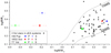 |
Fig. 16. Location of the primary (filled symbols) and secondary (empty symbols) components of HM Pup (points), V632 Sco (squares), and TT Vel (diamonds) within the mass-radius diagram. The star symbols denote the δ Scuti components of other oEA systems (taken from Liakos & Niarchos 2017), while the solid black lines represent the boundaries of the main sequence. |
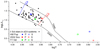 |
Fig. 17. Location of the components of the studied systems within the HR diagram. Symbols and solid black lines have the same meaning as in Fig. 16. The solid coloured lines (B = blue and R = red) denote the boundaries of the instability strip (IS; taken from Murphy et al. 2019). |
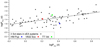 |
Fig. 18. Locations of the pulsating components of each studied system and other δ Scuti star members of oEA stars within the Porb − Ppul diagram. Symbols have the same meaning as in Fig. 16, while the solid line denotes the empirical fit of Liakos & Niarchos (2017). |
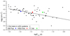 |
Fig. 19. Locations of the pulsating components of each studied system and other δ Scuti star members of oEA stars within the log g − Ppul diagram. The symbols and line have the same meaning as in Fig. 18. |
The primary components of each system lie in the centre of the main sequence within the instability strip (Fig. 17). The evolution of Algol binary systems, in which mass ratio reversal occurs, is complex and is not a topic of discussion in this paper. The primary component of V632 Sco is close to the red edge of the instability strip and the border with the γ Doradus stars (Uytterhoeven et al. 2011). This evolutionary position, together with the frequency analysis indicating a probable independent frequency in the 0–4 cycle d−1 range (Sect. 5.2), suggests that this star could have a δ Scuti-γ Doradus hybrid nature.
There is a relationship between the frequency of pulsations and the orbital period in close binary systems (c.f. Liakos & Niarchos 2017). The primary components of V632 Sco and TT Vel fit the trend calculated by Liakos & Niarchos (2017) quite well, whereas that of HM Pup deviates from it a little (Fig. 18). Furthermore, a relationship has been found between the pulsation period and the evolutionary stage (log g) of the δ Scuti-type components of close binary stars (Liakos & Niarchos 2017), although it is based on only a small sample of systems where RVs have been determined. The primaries of HM Pup and V632 Sco are very close to the empirical fit, while that of TT Vel shows a larger deviation.
The secondary components of each system are well above the terminal age on the main sequence (Figs. 16 and 17). Their derived log g values are 3.3–3.57 cm s−2 (Table 4), which indicates that all of them are in the subgiant or giant evolutionary phase of evolution. As the primary eclipse of HM Pup is total, with totality extending for 42 min, we were able to observe and classify the spectrum of its secondary component and confirm that it is a subgiant or giant, although smaller in size than typical single giant K8 stars.
7. Summary and conclusions
In this study we present a holistic and detailed analysis of three southern EBs with a pulsating component. Multi-filter ground-based photometric observations and TESS data were used. Moreover, spectroscopic observations were obtained allowing for the determination of the spectral types of the primaries of all systems and the secondary of HM Pup as well as the RVs of both components. The combination of these data provided the means for accurate photometric modelling followed by the determination of the physical parameters and the evolutionary stages of the components of the systems. Analysis of eclipse timings collected from the literature, and our observations, offered the opportunity to determine possible orbital period modulation mechanisms and quantify the mass transfer and mass loss rates, which were found in the spectra. The residuals of the LCs were analysed to detect pulsation frequencies. The frequencies detected in different wavelength bands were compared with each other in order to determine the oscillation modes of the pulsators. The primary components of the systems were identified as δ Scuti type stars based on their physical (i.e. Teff, M, and R) and pulsation properties (frequency ranges). All systems were found to be in a semi-detached configuration with the primaries being main-sequence stars and with the secondaries (cooler and less massive components), filling their Roche lobes and being in evolved evolutionary stages. Therefore, these systems are classical Algols (in terms of evolution) and are oEA stars according to the definition of Mkrtichian et al. (2002). The current status of these systems confirms the conclusion of Liakos & Niarchos (2017) regarding the earlier initiation of the pulsations due to the presence of a close companion.
The primary component of HM Pup pulsates in two independent frequencies at 36.4 and 38.6 cycle d−1, which are identified as p-mode oscillations. In total, 22 and 26 frequencies were detected in B filter and TESS data, respectively, but all except for the two above are combinations of other frequencies. The HM Pup orbital period has one cyclic variation which cannot be fully explained by the possible presence of a tertiary companion. No third light trace was detected in the analyses of light curves, Na I D spectra, or broadening function values. On the other hand, our results show that there is evidence for gas streaming from the secondary component and impacting on the primary component. The secondary component was found to be magnetically active and at a subgiant-giant phase of evolution.
The pulsating component of V632 Sco oscillates in two independent frequencies at 23.54 and 16.78 cycle d−1, which are independent non-radial pressure mode oscillations. More frequencies were detected (11 and 12 in the B filter and TESS data, respectively), but they are combinations of other frequencies. Another one was found in the slow-frequency regime, but its value was not exactly the same in all data sets; therefore, it might be an artefact. On the other hand, the location of the primary-pulsating component on the borders of δ Scuti-γ Doradus stars leaves the possibility open of a hybrid nature. The secular changes in the orbital period of the system indicate mass transfer from the secondary component at the rate of 2.1 × 10⁻⁸ M⊙ yr−1. As is the case for all three systems, mass flow from the secondary component is seen in the sodium doublet spectra. Furthermore, there is no evidence of a tertiary component in the sodium spectra, nor in the broadening function analyses. The secondary component was found to have an active spot migrating with a time period of a few days.
For the δ Scuti star of TT Vel, at least seven frequencies were detected in B, V, and I filters and more than 15 in the TESS data. However, only one (∼15.3 cycle d−1) was validated as a real independent frequency and is identified as a p-mode oscillation. The other potential independent frequencies were either not detected in all data sets or they are combinations of other frequencies. The secular changes in the orbital period can be explained with a mass transfer rate of 4.9 × 10⁻⁸ M⊙ yr−1. However, the current evolutionary status of the components gives rise to the possibility of mass loss from the system. The mass loss was calculated as −3 × 10⁻⁷ M⊙ yr−1, and probably both mechanisms occur with slower rates. The periodic changes of the orbital period might be due to the presence of a faint tertiary component.
More studies of similar systems are highly recommended. This will enrich the sample of oEA stars with accurately determined absolute properties. In turn, this will improve our knowledge of how interactions of components in close binary systems influence pulsations.
Acknowledgments
A.L. acknowledges financial support by the European Space Agency (ESA) under the Consolidating Activities Regarding Moon, Earth and NEOs (CARMEN) project, NOA/SRFA no. 1084 and wishes to thank Dr N. Nanouris for his valuable comments on the ETV analysis. D.J.W.M., M.G.B. and J.F.W. acknowledge grants for time on the ANU 2.3 m telescope from the Edward Corbould Research Fund of the Astronomical Association of Queensland. D.J.W.M. is grateful to Prof. Michael Drinkwater for his extensive assistance with the planning and data analysis of the ANU 2.3 m telescope observations. D.J.W.M. thanks A. Mohit, Y. Rist and L. Coetzee for their assistance with the spectroscopic observations. We thank the anonymous reviewer for the valuable comments that improved the quality of this work. This research has made use of NASA’s Astrophysics Data System Bibliographic Services, the SIMBAD database, operated at CDS, Strasbourg, France, the TIDAK database (B. Zakrzewski), the ‘O–C’ gateway database, and the Mikulski Archive for Space Telescopes (MAST). To the memory of Georgia and Eleftherios Stavrou aunt and uncle of AL.
References
- Aerts, C., Christensen-Dalsgaard, J., & Kurtz, D. W. 2010, Asteroseismology (Netherlands: Springer) [Google Scholar]
- Antoci, V., Cunha, M., Houdek, G., et al. 2014, ApJ, 796, 118 [Google Scholar]
- Applegate, J. H. 1992, ApJ, 385, 621 [Google Scholar]
- Applegate, J. H., & Patterson, J. 1987, ApJ, 322, L99 [NASA ADS] [CrossRef] [Google Scholar]
- Balona, L. A. 2014, MNRAS, 439, 3453 [NASA ADS] [CrossRef] [Google Scholar]
- Balona, L. A., Daszyńska-Daszkiewicz, J., & Pamyatnykh, A. A. 2015, MNRAS, 452, 3073 [Google Scholar]
- Baran, A. S., & Koen, C. 2021, Acta Astron., 71, 113 [Google Scholar]
- Baran, A. S., Koen, C., & Pokrzywka, B. 2015, MNRAS, 448, L16 [NASA ADS] [CrossRef] [Google Scholar]
- Berdyugina, S. V. 2005, Liv. Rev. Sol. Phys., 2, 8 [Google Scholar]
- Borucki, W. J., Koch, D., Basri, G., et al. 2010, Science, 327, 977 [Google Scholar]
- Bowman, D. M., & Kurtz, D. W. 2018, MNRAS, 476, 3169 [NASA ADS] [CrossRef] [Google Scholar]
- Bowman, D. M., & Michielsen, M. 2021, A&A, 656, A158 [NASA ADS] [CrossRef] [EDP Sciences] [Google Scholar]
- Bowman, D. M., Johnston, C., Tkachenko, A., et al. 2019, ApJ, 883, L26 [Google Scholar]
- Breger, M. 2000, in Delta Scuti and Related Stars, eds. M. Breger, & M. Montgomery, ASP Conf. Ser., 210, 3 [Google Scholar]
- Breger, M., Stich, J., Garrido, R., et al. 1993, A&A, 271, 482 [NASA ADS] [Google Scholar]
- Claret, A. 2018, A&A, 618, A20 [NASA ADS] [CrossRef] [EDP Sciences] [Google Scholar]
- Coelho, P., Barbuy, B., Meléndez, J., Schiavon, R. P., & Castilho, B. V. 2005, A&A, 443, 735 [NASA ADS] [CrossRef] [EDP Sciences] [Google Scholar]
- Collins, K. A., Kielkopf, J. F., Stassun, K. G., & Hessman, F. V. 2017, AJ, 153, 77 [Google Scholar]
- Cox, A. N. 2000, Allen’s Astrophysical Quantities (New York: Springer-Verlag) [Google Scholar]
- Dopita, M., Hart, J., McGregor, P., et al. 2007, Ap&SS, 310, 255 [Google Scholar]
- Dopita, M., Rhee, J., Farage, C., et al. 2010, Ap&SS, 327, 245 [Google Scholar]
- Drake, A. J., Djorgovski, S. G., Mahabal, A., et al. 2009, ApJ, 696, 870 [Google Scholar]
- Fitch, W. S. 1981, ApJ, 249, 218 [NASA ADS] [CrossRef] [Google Scholar]
- Gray, R. O., & Corbally, C. J. 2009, Stellar Spectral Classification (Princeton University Press) [Google Scholar]
- Gray, R. O., & Corbally, C. J. 2014, AJ, 147, 80 [CrossRef] [Google Scholar]
- Handler, G. 1999, MNRAS, 309, L19 [NASA ADS] [CrossRef] [Google Scholar]
- Henden, A. A., Levine, S., Terrell, D., & Welch, D. L. 2015, Am. Astron. Soc. Meeting Abstr., 225, 336.16 [Google Scholar]
- Hilditch, R. W. 2001, An Introduction to Close Binary Stars (Cambridge University Press) [Google Scholar]
- Hoffman, D. I., Harrison, T. E., McNamara, B. J., et al. 2006, AJ, 132, 2260 [NASA ADS] [CrossRef] [Google Scholar]
- Howell, S. B., Sobeck, C., Haas, M., et al. 2014, PASP, 126, 398 [Google Scholar]
- Irwin, J. B. 1959, AJ, 64, 149 [Google Scholar]
- Kalimeris, A., Rovithis-Livaniou, H., & Rovithis, P. 1994, A&A, 282, 775 [Google Scholar]
- Kim, S.-L., Lee, J. W., Lee, C.-U., et al. 2021, AJ, 162, 212 [NASA ADS] [CrossRef] [Google Scholar]
- Koch, D. G., Borucki, W. J., Basri, G., et al. 2010, ApJ, 713, L79 [Google Scholar]
- Kruszewski, A. 1966, Adv. Astron. Astrophys., 4, 233 [CrossRef] [Google Scholar]
- Kurtz, D. W., Handler, G., Rappaport, S. A., et al. 2020, MNRAS, 494, 5118 [Google Scholar]
- Lanza, A. F. 2006, MNRAS, 369, 1773 [NASA ADS] [CrossRef] [Google Scholar]
- Lanza, A. F. 2020, MNRAS, 491, 1820 [NASA ADS] [Google Scholar]
- Lanza, A. F., & Rodonò, M. 2002, Astron. Nachr., 323, 424 [NASA ADS] [CrossRef] [Google Scholar]
- Lanza, A. F., Catalano, S., Cutispoto, G., Pagano, I., & Rodono, M. 1998, A&A, 332, 541 [NASA ADS] [Google Scholar]
- Lenz, P., & Breger, M. 2005, Commun. Asteroseismol., 146, 53 [Google Scholar]
- Liakos, A. 2015, in Living Together: Planets, Host Stars and Binaries, eds. S. M. Rucinski, G. Torres, & M. Zejda, ASP Conf. Ser., 496, 286 [Google Scholar]
- Liakos, A. 2017, A&A, 607, A85 [NASA ADS] [CrossRef] [EDP Sciences] [Google Scholar]
- Liakos, A. 2018, A&A, 616, A130 [NASA ADS] [CrossRef] [EDP Sciences] [Google Scholar]
- Liakos, A. 2020a, Acta Astron., 70, 265 [NASA ADS] [Google Scholar]
- Liakos, A. 2020b, A&A, 642, A91 [NASA ADS] [CrossRef] [EDP Sciences] [Google Scholar]
- Liakos, A., & Cagaš, P. 2014, Ap&SS, 353, 559 [NASA ADS] [CrossRef] [Google Scholar]
- Liakos, A., & Niarchos, P. 2013, Ap&SS, 343, 123 [NASA ADS] [CrossRef] [Google Scholar]
- Liakos, A., & Niarchos, P. 2017, MNRAS, 465, 1181 [NASA ADS] [CrossRef] [Google Scholar]
- Liakos, A., & Niarchos, P. 2020, Galaxies, 8, 75 [NASA ADS] [CrossRef] [Google Scholar]
- Liakos, A., Zasche, P., & Niarchos, P. 2011, New A, 16, 530 [NASA ADS] [CrossRef] [Google Scholar]
- Liakos, A., Niarchos, P., Soydugan, E., & Zasche, P. 2012, MNRAS, 422, 1250 [Google Scholar]
- Lucy, L. B. 1967, ZAp, 65, 89 [NASA ADS] [Google Scholar]
- Mkrtichian, D. E., Kusakin, A. V., Gamarova, A. Y., & Nazarenko, V. 2002, in IAU Colloq. 185: Radial and Nonradial Pulsationsn as Probes of Stellar Physics, eds. C. Aerts, T. R. Bedding, & J. Christensen-Dalsgaard, ASP Conf. Ser., 259, 96 [Google Scholar]
- Mkrtichian, D. E., Lehmann, H., Rodríguez, E., et al. 2018a, MNRAS, 475, 4745 [NASA ADS] [CrossRef] [Google Scholar]
- Mkrtichian, D. E., Gunsriwiwat, K., Reichart, D. E., et al. 2018b, Inf. Bull. Var. Stars, 6238, 1 [NASA ADS] [Google Scholar]
- Montalbán, J., & Dupret, M. A. 2007, A&A, 470, 991 [NASA ADS] [CrossRef] [EDP Sciences] [Google Scholar]
- Moriarty, D. J. W., Bohlsen, T., Heathcote, B., Richards, T., & Streamer, M. 2013, JAAVSO, 41, 182 [NASA ADS] [Google Scholar]
- Moriarty, D. J. W., Liakos, A., Drinkwater, M. J., et al. 2019, Ap&SS, 365, 1 [Google Scholar]
- Murphy, S. J., Pigulski, A., Kurtz, D. W., et al. 2013, MNRAS, 432, 2284 [NASA ADS] [CrossRef] [Google Scholar]
- Murphy, S. J., Hey, D., Van Reeth, T., & Bedding, T. R. 2019, MNRAS, 485, 2380 [NASA ADS] [CrossRef] [Google Scholar]
- Nelson, R. H. 2005, B-Minima [Google Scholar]
- Ogloza, W., Stachowski, G., Zakrzewski, B., & Zejmo, M. 2022, in TIDAK: the updated Suhora database of O−C diagrams and elements of eclipsing binary stars, XL Polish Astronomical Society Meeting proc, 123 [Google Scholar]
- Pilecki, B., Gieren, W., Smolec, R., et al. 2017, ApJ, 842, 110 [Google Scholar]
- Pojmanski, G. 2002, Acta Astron., 52, 397 [NASA ADS] [Google Scholar]
- Prša, A., & Zwitter, T. 2005, ApJ, 628, 426 [Google Scholar]
- Richards, M. T., & Albright, G. E. 1999, ApJS, 123, 537 [NASA ADS] [CrossRef] [Google Scholar]
- Ricker, G. R., Latham, D. W., Vanderspek, R. K., et al. 2009, in Am. Astron. Soc. Meeting Abstr., 213, 403.01 [NASA ADS] [Google Scholar]
- Ricker, G. R., Winn, J. N., Vanderspek, R., et al. 2015, J. Astron. Telesc. Instrum. Syst., 1, 014003 [Google Scholar]
- Rovithis-Livaniou, H., Kranidiotis, A. N., Rovithis, P., & Athanassiades, G. 2000, A&A, 354, 904 [NASA ADS] [Google Scholar]
- Ruciński, S. M. 1969, Acta Astron., 19, 245 [Google Scholar]
- Ruciński, S. M. 1992, AJ, 104, 1968 [CrossRef] [Google Scholar]
- Ruciński, S. M. 2002, AJ, 124, 1746 [CrossRef] [Google Scholar]
- Shappee, B., Prieto, J., Stanek, K. Z., et al. 2014, in Am. Astron. Soc. Meeting Abstr., 223, 236.03 [NASA ADS] [Google Scholar]
- Soydugan, F., Soydugan, E., Kanvermez, Ç., & Liakos, A. 2013, MNRAS, 432, 3278 [NASA ADS] [CrossRef] [Google Scholar]
- Stassun, K. G., Oelkers, R. J., Paegert, M., et al. 2019, AJ, 158, 138 [Google Scholar]
- Streamer, M., Bohlsen, T., & Ogmen, Y. 2016, JAAVSO, 44, 39 [NASA ADS] [Google Scholar]
- Ulaş, B., Gazeas, K., Liakos, A., et al. 2020, Acta Astron., 70, 219 [Google Scholar]
- Uytterhoeven, K., Moya, A., Grigahcène, A., et al. 2011, A&A, 534, A125 [CrossRef] [EDP Sciences] [Google Scholar]
- van Hamme, W. 1993, AJ, 106, 2096 [Google Scholar]
- Völschow, M., Schleicher, D. R. G., Banerjee, R., & Schmitt, J. H. M. M. 2018, A&A, 620, A42 [NASA ADS] [CrossRef] [EDP Sciences] [Google Scholar]
- von Zeipel, H. 1924, MNRAS, 84, 665 [NASA ADS] [CrossRef] [Google Scholar]
- Wilson, R. E. 1979, ApJ, 234, 1054 [Google Scholar]
- Wilson, R. E. 1990, ApJ, 356, 613 [Google Scholar]
- Wilson, R. E., & Devinney, E. J. 1971, ApJ, 166, 605 [Google Scholar]
- Zasche, P., Liakos, A., Niarchos, P., et al. 2009, New A, 14, 121 [NASA ADS] [CrossRef] [Google Scholar]
- Zima, W. 2008, Commun. Asteroseismol., 157, 387 [NASA ADS] [Google Scholar]
Appendix A: Radial velocities
This appendix includes the heliocentric RV measurements of the studied systems. Details regarding the calculation method of the RVs are given in Section 3.
Radial velocity measurements. The columns contain the heliocentric Julian date of the observations and the RVs of the components of the systems (1=primary and 2=secondary).
Appendix B: Gas velocities of HM Pup
This appendix (Table B.1) includes – for various orbital phases of HM Pup – the velocities of the primary component (V1), based on the centred wavelength (λ1) of its Na I D line, the centred wavelength of the line of the gas (λgas), and its corresponding velocity (Vgas) as well as the relative velocity of the gas to the primary component (V1, gas). The wavelengths and velocities were adjusted, for clarity, to remove the fixed systemic velocity of 58 km s−1.
Velocities of the HM Pup primary star and wavelengths and velocities of its Na I D lines and the gas stream from the secondary star at a range of orbital phases (with systemic velocity subtracted).
Appendix C: Spots
The location of the spots on the secondary components of the systems, assumed in the LC and RV modelling (Section 3), are given in Table C.1.
Spot location on the surface of the secondary components. The columns include the passbands used for modelling LCs and RVs, the number of spots for each model, and the parameters of the spots (Co-latitude, longitude, radius, and temperature factor). The letter ‘G’ given for the models of V632 Sco using the TESS data stands for group of LCs (see Section 3 for details).
Appendix D: Times of minima
Table D.1 hosts the times of minima calculated from personal ground-based observations and the available data from the TESS mission. In cases where two or more filters are listed for a given minimum time, the latter is the average of the times of minima calculated for the data of each filter. More details about the calculation method are given in Section 4.
Times of minima derived from the ground-based and TESS data. The columns contain the heliocentric Julian date and the type (I=primary eclipse and II=secondary eclipse) of each minimum and the filters used for the individual observations.
Table D.1 cont.
Appendix E: Complete pulsation models
This appendix contains three tables which list the detected frequencies in all available data sets for each system. Details about the frequency analysis can be found in Section 5.
Detected pulsation frequencies of the δ Scuti component of HM Pup in all data sets. The columns contain the increasing number (n), the value (fn), the amplitude (A), the phase (Φ), the S/N, and the most possible combination of each detected frequency.
Table E.1 cont.
Same as Table E.1, but for V632 Sco.
Same as Table E.1, but for TT Vel.
All Tables
Independent pulsation frequencies and MAD model results for the δ Scuti stars in each system.
Radial velocity measurements. The columns contain the heliocentric Julian date of the observations and the RVs of the components of the systems (1=primary and 2=secondary).
Velocities of the HM Pup primary star and wavelengths and velocities of its Na I D lines and the gas stream from the secondary star at a range of orbital phases (with systemic velocity subtracted).
Spot location on the surface of the secondary components. The columns include the passbands used for modelling LCs and RVs, the number of spots for each model, and the parameters of the spots (Co-latitude, longitude, radius, and temperature factor). The letter ‘G’ given for the models of V632 Sco using the TESS data stands for group of LCs (see Section 3 for details).
Times of minima derived from the ground-based and TESS data. The columns contain the heliocentric Julian date and the type (I=primary eclipse and II=secondary eclipse) of each minimum and the filters used for the individual observations.
Detected pulsation frequencies of the δ Scuti component of HM Pup in all data sets. The columns contain the increasing number (n), the value (fn), the amplitude (A), the phase (Φ), the S/N, and the most possible combination of each detected frequency.
All Figures
|
Fig. 1. TESS LCs that cover approximately 26 days of continuous monitoring. The rest of the data are not shown for scaling reasons. The time resolution of the data sets is 10, 2, and 10 min for HM Pup (top), V632 Sco (middle), and TT Vel (bottom), respectively. |
| In the text | |
|
Fig. 2. Rectified spectra of the primary components of each system and the secondary component of HM Pup. |
| In the text | |
|
Fig. 3. Examples of broadening functions analyses on the spectra of (a) HM Pup at phase 0.25, (b) V632 Sco at phase 0.25, and (c) TT Vel at phase 0.75. Blue lines denote the RVs of the primary and red lines those of the secondary components. |
| In the text | |
|
Fig. 4. Spectra of the HM Pup secondary star in the range 3900–4020 Å (with R = 3000) during totality on two occasions. The K and H emission peaks have a red shift of 58 km s−1. |
| In the text | |
|
Fig. 5. Hα (a) and Na I D (b) spectra of the HM Pup secondary star observed at the same time as the Ca II spectra in Fig. 4, but with R = 7000. Arrows mark the calculated wavelength positions of the spectral line centres at the systemic velocity. |
| In the text | |
|
Fig. 6. Spectra of HM Pup Na I D lines at several orbital phases (Φ) with R = 7000. Downward arrows mark the calculated position of the line centres for the primary star that are the sum of the systemic and orbital velocities. Lines of circumstellar gas are marked with blue arrows. |
| In the text | |
|
Fig. 7. Spectra of Na I D lines at quadrature phases (R = 7000): (a, b) V632 Sco and (c, d) TT Vel. Downward arrows mark the calculated position of the line centres for primary components that are the sum of their orbital and systemic velocities. |
| In the text | |
|
Fig. 8. Illustration of the method used to estimate the wavelength of the D2 line of the gas at phase 0.28. The primary star absorption line is long-dashed, and the gas is short-dashed. |
| In the text | |
|
Fig. 9. Estimated path of the HM Pup gas stream. The phases of the observations are marked around the periphery of the dashed circle, and the corresponding observed gas velocity and direction relative to the primary star are indicated inside the circle. The orbital direction and direction of rotation of the two stars are shown by the long-dashed and short-dashed arrows, respectively. The wavelengths and velocities were adjusted, for clarity, to remove the fixed systemic velocity of 58 km s−1. |
| In the text | |
|
Fig. 10. Synthetic (solid lines) over observed (points) LCs (left plots) and RVs (right plots) for HM Pup (top panels), V632 Sco (middle panels), and TT Vel (bottom panels). Some LCs were vertically shifted for scaling reasons. The fit on the out-of-primary eclipse points of the B filter was re-scaled and plotted allowing for better viewing. |
| In the text | |
|
Fig. 11. Eclipse timing variations plot for HM Pup. Top panel: O–C points of the system fitted by a LITE curve (upper part) and the residuals (lower part) of the fit. For both panels, the bigger the symbol is, the bigger the statistical weight of the individual points. |
| In the text | |
|
Fig. 12. Eclipse timing variations plots for V632 Sco. Top panel: O–C points of the system fitted by a parabola (upper part) and the residuals (lower part) of the fit. Bottom panel: same as previous panel, but with the fit of a parabolic and LITE curves. |
| In the text | |
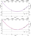 |
Fig. 13. Same as Fig. 12, but for TT Vel. |
| In the text | |
|
Fig. 14. Representative Fourier fit on the data of B filter and TESS. |
| In the text | |
|
Fig. 15. Periodograms of B filter (left panels) and TESS data (right panels). Some of the detected strong frequencies are indicated. |
| In the text | |
|
Fig. 16. Location of the primary (filled symbols) and secondary (empty symbols) components of HM Pup (points), V632 Sco (squares), and TT Vel (diamonds) within the mass-radius diagram. The star symbols denote the δ Scuti components of other oEA systems (taken from Liakos & Niarchos 2017), while the solid black lines represent the boundaries of the main sequence. |
| In the text | |
|
Fig. 17. Location of the components of the studied systems within the HR diagram. Symbols and solid black lines have the same meaning as in Fig. 16. The solid coloured lines (B = blue and R = red) denote the boundaries of the instability strip (IS; taken from Murphy et al. 2019). |
| In the text | |
|
Fig. 18. Locations of the pulsating components of each studied system and other δ Scuti star members of oEA stars within the Porb − Ppul diagram. Symbols have the same meaning as in Fig. 16, while the solid line denotes the empirical fit of Liakos & Niarchos (2017). |
| In the text | |
|
Fig. 19. Locations of the pulsating components of each studied system and other δ Scuti star members of oEA stars within the log g − Ppul diagram. The symbols and line have the same meaning as in Fig. 18. |
| In the text | |
Current usage metrics show cumulative count of Article Views (full-text article views including HTML views, PDF and ePub downloads, according to the available data) and Abstracts Views on Vision4Press platform.
Data correspond to usage on the plateform after 2015. The current usage metrics is available 48-96 hours after online publication and is updated daily on week days.
Initial download of the metrics may take a while.