| Issue |
A&A
Volume 663, July 2022
|
|
|---|---|---|
| Article Number | A17 | |
| Number of page(s) | 16 | |
| Section | Cosmology (including clusters of galaxies) | |
| DOI | https://doi.org/10.1051/0004-6361/202040238 | |
| Published online | 04 July 2022 | |
Triaxiality in galaxy clusters: Mass versus potential reconstructions
1
Institut für Theoretische Physik, Heidelberg University, Philosophenweg 16, 69120 Heidelberg, Germany
e-mail: This email address is being protected from spambots. You need JavaScript enabled to view it.
2
Institut für Theoretische Astrophysik, Zentrum für Astronomie, Heidelberg University, Philosophenweg 12, 69120 Heidelberg, Germany
3
Department of Physics, University of Miami, Coral Gables, FL, 33124
USA
4
Center for Astrophysics, Harvard & Smithsonian, 60 Garden St, Cambridge, MA, 02138
USA
Received:
24
December
2020
Accepted:
4
April
2022
Abstract
Context. Accounting for the triaxial shapes of galaxy clusters will become important in the context of upcoming cosmological surveys. This will provide a challenge given that the density distribution of gas cannot be described by simple geometrical models without loss of information.
Aims. We investigate the effects of simple 3D models on cluster gravitational potentials and gas density distribution to determine which of these quantities is most suitable and appropriate for characterising galaxy clusters in cosmological studies.
Methods. We use a statistical sample of 85 galaxy clusters from a large cosmological N-body + hydrodynamical simulation to investigate cluster shapes as a function of radius for both gas density and potential. We examine how the resulting parameters are affected by the substructure removal (for the gas density) and by the definition of the computation volume (interior vs. shells).
Results. We find that the orientation and axis ratio of gas isodensity contours are degenerate with the presence of substructures and are unstable against fluctuations. Moreover, as the derived cluster shape depends on the method used for removing the substructures, thermodynamic properties extracted from the X-ray emissivity profile, for example, suffer from this additional and often underestimated bias. In contrast, the shapes of the smooth cluster potentials are less affected by fluctuations and converge towards simple geometrical models, both in the case of relaxed and dynamically active clusters.
Conclusions. The observation that cluster potentials can be represented better by simple geometrical models and reconstructed with a lower level of systematic error for both dynamically active and relaxed clusters suggests that characterising galaxy clusters by their potential is a promising alternative to using cluster masses in cluster cosmology. With this approach, dynamically active and relaxed clusters could be combined in cosmological studies, improving statistics and lowering scatter.
Key words: galaxies: clusters: general / cosmology: observations / X-rays: galaxies: clusters / methods: data analysis
© S. Stapelberg et al. 2022
 Open Access article, published by EDP Sciences, under the terms of the Creative Commons Attribution License (https://creativecommons.org/licenses/by/4.0), which permits unrestricted use, distribution, and reproduction in any medium, provided the original work is properly cited.
This article is published in open access under the Subscribe-to-Open model. This email address is being protected from spambots. You need JavaScript enabled to view it. to support open access publication.
1. Introduction
The statistics of the galaxy cluster population as a function of redshift and mass is often used to trace the evolution of large-scale structures (see e.g. Voit 2005; Planck Collaboration XIII 2016). Such cosmological probes require well-constrained cluster mass estimates for comparison with theoretical predictions. The X-ray bremsstrahlung emission (e.g. Sarazin 1988; Eckert et al. 2019), the signal from the thermal Sunyaev-Zel’dovich effect (tSZ, e.g. Sunyaev & Zeldovich 1969; Sayers et al. 2011), and gravitational lensing measurements (e.g. Bartelmann 2010; Jauzac et al. 2019) are typical mass proxies based on the assumption that the cluster matter distribution can be described by a simple spherical or spheroidal1 model2. In addition, cosmological studies are often based on scaling relations derived from a sample of relaxed clusters selected for being almost spherical and in hydrostatic equilibrium (Vikhlinin et al. 2009; Mantz et al. 2016). Pratt et al. (2019), for example, recently published a thorough review of the past and ongoing efforts to derive cosmological constraints using the subsample of relaxed clusters in order to tighten the existing mass-observable scaling relations (see their Sect. 4.5). These estimates are then compared to theoretical predictions that have been derived for these same simple geometrical models (e.g. the spherical collapse model; see Press & Schechter 1974; Tozzi & Norman 2001; Voit 2005, for some applications).
However, both simulations and observations have demonstrated for decades that the shape of isodensity contours in clusters is non-spherical and can deviate largely from spheroidicity as well (see e.g. Limousin et al. 2013 for a review). Cosmological simulations predict the formation of triaxial dark matter haloes (e.g. Jing & Suto 2002) as a consequence of the anisotropic gravitational collapse for a Gaussian random field of primordial density fluctuations. This also affects the relaxed clusters, whose shape can vary with radius (e.g. Dubinski & Carlberg 1991; Allgood et al. 2006; Vera-Ciro et al. 2011; Harvey et al. 2019). At the same time, cluster shapes depend on mass, with higher mass haloes being less spherical than lower mass haloes (e.g. Kasun & Evrard 2005; Allgood et al. 2006; Bett et al. 2007). Depending on the selected cluster sample, different cosmological results may be obtained. Thus, accounting for the most precise cluster shape is crucial. Being the most massive bound objects, galaxy clusters formed latest in cosmic history and represent a population that is, at least in parts, out of dynamical equilibrium (e.g. Gao et al. 2012; Bartelmann et al. 2013). Cosmological simulations suggest that the morphologies of cluster haloes are closely linked to the formation history of the galaxy clusters (Evrard et al. 1993; Suto et al. 2016; Lau et al. 2021). Their axial ratios are sensitive to σ8 and (weakly) to Ωm (see e.g. Buote & Humphrey 2012, and references therein) and are expected to be closer to unity if dark matter is self-interacting (e.g. Davé et al. 2001; Peter et al. 2013; Banerjee et al. 2020).
In the context of upcoming cosmological studies, taking into account the three-dimensional (3D) cluster shapes and their influence on the reconstruction of cluster quantities is going to be critical (e.g. Limousin et al. 2013). Observational mass biases arising from the symmetry assumption are already well documented (see e.g. Rasia et al. 2012). Due to the dependence of the X-ray emissivity on the squared gas density and on the steep slope of gas density, the cluster morphology derived from X-rays appears typically more spherical than it would if it were derived from other observables (combining different observational probes is necessary to constrain the cluster shape; e.g. Morandi et al. 2010, 2012; Limousin et al. 2013; Sereno et al. 2018). In addition, the presence of substructures may lead to underestimation of the total hydrostatic mass (HE mass) derived from X-rays (e.g. Ettori et al. 2013). A dedicated analysis of the effect of the assumed symmetry on the results obtained from hydrostatic equilibrium can be found in Chiu & Molnar (2012). Regarding gravitational lensing measurements, cluster masses derived under the assumption of spherical symmetry may be over- or underestimated depending on the orientation of the principal axis of the lens mass distribution with respect to the line of sight (Meneghetti et al. 2010; Osato et al. 2018; Lee et al. 2018).
Contrary to most of the studies listed above and to the analysis performed in Buote & Humphrey (2012) – where the authors computed the orientation-averaged biases arising when masses of ellipsoidal clusters are estimated assuming spherical symmetry –, in the present study, we do not assume that the density distribution is stratified in ellipsoids of constant axis ratio and orientation, as this is clearly not the case. Instead, we are interested in the variation of the shape of isodensity layers with cluster-centric distance. We investigate the impact of asymmetries, fluctuations, and substructure-removal methods on the shape of these isodensity layers. Substructures are clumps of matter that are not yet in virial equilibrium with the cluster gravitational potential. This implies that their temperature, metallicity, and density are not representative of the surrounding intracluster medium (ICM), and therefore that they should be removed from the analysis if we wish to derive bulk properties such as the hydrostatic mass. This step is particularly important for the treatment of X-ray observations, as the signal emitted by these density inhomogeneities is enhanced relative to the signal from the ICM gas (e.g. Ettori et al. 2013).
Modelling the 3D morphology of a cluster from 2D observations is complicated by projection effects arising from the unknown orientation angle and the intrinsic ellipticity of the cluster, but also from the contribution of the substructures. We show here that this task is not trivial because of ambiguities even if we have at hand the full 3D density distribution of simulated clusters. For example, substructure removal is performed for an assumed cluster morphology and this, in turn, biases the resulting density distribution, as can be observed when using the azimuthal median method to remove substructures (Eckert et al. 2015): in each spherical shell, the median is used instead of the mean. While being very efficient for spherically symmetric clusters (Zhuravleva et al. 2013), we saw in our companion study (Tchernin et al. 2020) that applying this method to an elliptical cluster biases low the resulting profile (even for a cluster with small ellipticity; see Fig. A.8 of that study). However, there also exist less stringent selection criteria to identify substructures in spherical shells, such as the X-σ criterion, where X corresponds to a density threshold above which the pixels with larger density values are excluded from the analysis (e.g. X = 3.5 is used in Zhuravleva et al. 2013; Lau et al. 2015).
Here, we investigate the 3D shapes of a statistical sample of simulated galaxy clusters drawn from a cosmological hydrodynamic simulation. This includes a reference sample of 32 relaxed clusters, for which we explore several parameters of our shape determination methods, and an additional sample of 53 non-relaxed clusters, for which we measure shapes with the best working set of parameters. We show that removing substructures for an assumed spherical symmetry significantly affects the shape of the gas density distribution and should therefore be carefully taken into account in the systematic errors of the extracted mass profiles. In particular, in Sect. 3 we show that the analysis of the principal axes of the gas density distribution is heavily affected by the presence of fluctuations and by the specific choice of substructure-removal technique, even for relaxed clusters. We demonstrate that the distribution of the gravitational potential, in contrast, can be described by a simpler morphology and that fitting the potential isocontours is much more robust against the presence of local fluctuations and perturbations. We also note that differences in methodical details, such as the definition of the integration domain, have a smaller impact on the potential due to its simple geometry.
The gravitational potential contains all relevant information on the cluster morphology and can be related straightforwardly to a large number of multi-wavelength observables including X-ray, SZ, gravitational lensing, and galaxy kinematics, which allow for a joint reconstruction of cluster potentials (Konrad et al. 2013; Sarli et al. 2014; Tchernin et al. 2015; Stock et al. 2015; Majer et al. 2016). We discuss our results and their implications in Sect. 4 and conclude with the advantages of using the gravitational potential in Sect. 5.
2. Simulation and methods
2.1. Cosmological simulations
In this study, we use a statistical sample of 85 galaxy clusters extracted from the non-radiative hydrodynamic cosmological simulation OMEGA500 (Nelson et al. 2014), which was specially designed for studying galaxy clusters and also used in the companion paper (Tchernin et al. 2020). OMEGA500 was performed using the Eulerian ADAPTIVE REFINEMENT TREE (ART) N-body+gas-dynamics code (Kravtsov 1999; Rudd et al. 2008), adopting a flat ΛCDM cosmology with H0 = 70 km s−1 Mpc−1, Ωm = 0.27, ΩΛ = 0.73, Ωb = 0.0469, and σ8 = 0.82. The evolution of dark matter and gas was followed on an adaptive grid with a co-moving box size length of 500 Mpc h−1, resolved using a uniform 5123 root grid with eight levels of mesh refinement. Clusters were identified using a halo finder that detects mass peaks on a given scale and then performs an iterative search for the centre of mass (see Nelson et al. 2012, for details). The full sample of clusters consists of 85 objects at z = 0 with masses M200c ≳ 1.94 × 10¹⁴ h−1 M⊙, shown in a histogram in Fig. 1.
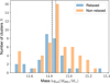 |
Fig. 1. Distributions of virial masses for the 85 simulated clusters of the OMEGA500 sample used in this work, subdivided into the relaxed and non-relaxed samples. The vertical lines mark the corresponding median values (dashed: relaxed, dotted: non-relaxed). |
We divide this cluster sample into ‘relaxed’ and ‘non-relaxed’ clusters based on the structural morphology of their X-ray images according to the ‘symmetry–peakiness–alignment’ (SPA) criterion by Mantz et al. (2015). This criterion applies cuts in three shape parameters referring to the regularity of X-ray isophotes, and has previously been applied to mock Chandra maps of the OMEGA500 clusters (Shi et al. 2016; Tchernin et al. 2020). This classification results in 32 relaxed and 53 unrelaxed clusters. Its purpose is to study the impact of the dynamical state of the clusters, which is expected to correlate with the deviation from sphericity. For both categories of clusters, we carry out the same analysis and comparisons.
In our previous study, we derived the systematic errors of the potential and HE mass for the OMEGA500 clusters, assuming spherical symmetry (Tchernin et al. 2020). We observed that the reconstructed potential is less affected by this simplifying assumption than the HE mass. We now go one step further and study the cluster morphology using the entire gas density distribution. We show in Sect. 3 that the gas density distribution ρg(x) in such galaxy clusters cannot be approximated with simple geometrical models and is significantly affected by the presence of substructures and fluctuations in the bulk gas density. We then compare these results to the cluster morphological information extracted using the potential distribution Φ(x).
2.2. Substructure removal
The triaxiality of clusters is degenerate with the presence of substructures. Substructures are gas-rich subhaloes of matter that are not yet in virial or hydrostatic equilibrium with the gravitational potential. The impact of these substructures must be taken into account when estimating the profiles or 3D shapes of clusters based on observables related to the gas density distribution, such as X-ray emissivity (e.g. Lau et al. 2015). In particular, to avoid large systematic biases for example in the ellipticity of cluster shapes, the contributions caused by inhomogeneities need to be removed from the signal of the bulk gas component. The bulk properties are in fact those relevant for characterising galaxy clusters – whether by their mass or their gravitational potential – under the assumption of hydrostatic equilibrium.
In Tchernin et al. (2020), we considered two methods for removal of the impact of substructures, namely the X-σ criterion and the median method. While the median method replaces the density distribution by its median in spherical shells, the X-σ criterion (Zhuravleva et al. 2013) preserves the 3D cluster shape information by using the shape of the logarithmic probability density distribution. The density distribution in spherical shells can be described by a log-normal function corresponding to a nearly hydrostatic bulk component, and a high-density tail caused by substructure-induced inhomogeneities. For illustration, an example of this is shown for the relaxed cluster CL1 in Fig. 2. The X-σ method removes gas cells with a logarithmic density of a factor X times σ above the median, which are assigned to the high-density tail:
 (1)
(1)
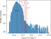 |
Fig. 2. Illustration of the X-sigma method. Shown are gas density values of the relaxed cluster CL1 in an arbitrary, thin spherical shell of width Δr ≈ 11 kpc between r500 and r200 (this is an example choice for illustration only). The dashed line shows the median density, while the blue solid line shows the threshold for X = 3.5. The red solid lines show further arbitrary example choices (X = 2, 3, 4) to give an impression of the extent to which variations of order unity in X affect the distribution. |
Here, σ is the log10-based standard deviation of the density distribution. The specific choice for X controls how sharp the cut will be. A typical empirically motivated value used in the literature is X = 3.5 (Zhuravleva et al. 2013; Lau et al. 2015). However, slightly higher or lower values might be equally viable given the relatively smooth transition between the log-normal component and the high-density tail. A few example values are shown in Fig. 2. For the computation of shape parameters, we substitute the holes left by masking substructures in two different ways by substituting (a) the median gas density at that cluster-centric radius, as was done by Chen et al. (2019); and (b) the threshold density value. While the former choice is representative of the distribution of gas density values within spherical shells, the latter preserves continuity and intrinsic asymmetries of the cluster at the expense of possibly overestimated gas density values at the positions of substructures. We apply and test the outcomes of both methods throughout this work.
For the cut parameter X, aside from the aforementioned reference value of X = 3.5, we also apply a slightly stricter and a less strict threshold X ∈ {3, 4} to study the impact of X. In addition, we include the choice X = 2.0, for which we saw in Tchernin et al. (2020) that this produces a mean density profile more similar to that of the median method. We thus obtain four distinct ‘cleaned’ simulation sets, which we refer to as 2S, 3S, 3.5S (or ‘reference’), and 4S, respectively. For each of these data sets, we apply and study both filling methods (a) and (b) to compare their impact on the 3D cluster morphologies. For comparisons with the gravitational potential distribution, we furthermore distinguish between two different representations of the potential data set: (i) the ‘raw’ non-processed potential of the cluster including all subclump contributions; and (ii) a version in which the regions identified as containing substructures are replaced by the median potential in the same fashion as for the gas density filling method (a). This latter version puts emphasis on methodical consistency while the former comparison (i.e. between substructure-cleaned gas density and raw potential) is interesting because it contrasts the optimum we can hope to achieve with the gas density (in terms of a smooth estimator of the intrinsic shape) after pre-processing it with the result we can expect from the unprocessed potential.
We note that the prevalence of substructures is expected to be highest in the outer regions, e.g. close to r500, which are dynamically younger and still show ongoing accretion of matter (e.g. Nagai & Lau 2011; Roncarelli et al. 2013; Vazza et al. 2013). Nonetheless, applying substructure-removal techniques can introduce uncertainties in the definition of cluster shapes at any radii. Moreover, there is no sharp distinction between inhomogeneities due to non-virialised gas clumps and intrinsic asymmetries of the bulk gas component. As a result, substructures and triaxiality can be highly degenerate (cf. Fig. 3), and the removal of substructures, which is always required for the gas density but may not be required for the potential, may artificially bias cluster shapes towards sphericity. Using all the different aforementioned data sets, we investigate the robustness of cluster shapes with respect to the value of X, the influence of removing or replacing the pixels, and the sensitivity to residual density fluctuations3 in the ‘bulk’ gas component.
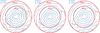 |
Fig. 3. Illustration of the substructure–triaxiality degeneracy: the figure shows 2D projected gas density isocontours of the simulated, average-mass relaxed cluster CL85, which we have picked here because its major axis is almost perpendicular to the viewing direction. Black: density isocontours after substructure removal for different choices. Blue dashed: original isocontours. While X = 3.5 does not remove all substructures, the stricter choice X = 2 also removes ellipticity from contours in the bulk within r500. |
2.3. Cluster shape definitions
We now describe the methods used to analyse the shape of the simulated clusters. An ellipsoidal body can be defined by its three principal axes a ≥ b ≥ c, while the orientation of the axis of longest elongation will be denoted by an angle vector ϕ. For characterising the shape itself, only two axis ratios are required. For a general mass or potential distribution ρ, the principal axis vectors are related to the eigenvectors of the mass tensor4,
 (2)
(2)
for a given volume V, where x is the position vector with respect to the centroid of the mass distribution. For the discrete data cubes provided by the simulations, the integral in Eq. (2) turns into a sum over grid pixels. This sum can be computed numerically and the resulting matrix Mij can be diagonalised to obtain its eigenvectors and eigenvalues.
In order to characterise the cluster shape, we define the ellipticity ϵ and the aspheroidicity A as
 (3)
(3)
 (4)
(4)
where a ≥ b ≥ c are the three principal axis lengths that correspond to the three eigenvalues λ1, λ2, λ3 of the mass tensor,  ,
,  ,
,  . We note that b = c describes the case of a spheroid. The ellipsoidal parametrisation of shapes for the cluster gas and potential distributions is motivated by earlier theoretical studies suggesting that the isopotential surfaces of dark matter haloes are well approximated by triaxial ellipsoids even for mass distributions that are ellipsoidal themselves (e.g. Lee & Suto 2003; Hayashi et al. 2007).
The morphology of a cluster is generally expected to evolve with the distance from the cluster centre (e.g. Allgood et al. 2006). This radial dependence of the cluster shape may contain potentially interesting information about the history of cluster formation, as the geometry of different layers is sensitive to cosmology and structure growth at different epochs (e.g. Lau et al. 2021). In this work we study the cluster shape evolution as a function of radius. This is done by computing the mass tensor for different ‘density layers’ (or potential layers) of each cluster individually, which allows us to obtain profiles of the shape parameters of interest, using the generalised radius r defined in Eq. (5). We start by binning the gas and potential distributions into isodensity (isopotential) shells of constant width in logarithmic space. The width of each bin is set to Δ(lnρ) = ln(ρi + 1/ρi) = 0.05 for the gas density and Δ(lnρ) = 0.02 for the potential. These values are arbitrary choices motivated by the requirement that the resulting shells be both large enough compared to the pixel size given by the finite resolution of the simulation, and small enough to still obtain smooth radial profiles. We verified through testing that small variations in the bin width do not influence our results and conclusions (see also Sect. 4.3, where we comment further on this).
For each bin, we apply two different methods for determining the shape of the cluster, which differ from each other by computing the integral in Mij over different domains: (1) over the corresponding thin shell only (ρ = const.) to define a ‘local’ shape measure; or (2) over the entire ‘inner’ spatial volume enclosed by the shell (including the shell itself), such that each bin effectively acts as an overdensity threshold, defining a region in which the shape of the enclosed cluster mass is measured. An illustration of the two approaches is given in Fig. 4. For brevity, we refer to these two variants respectively as the ‘local’ and ‘inner’ method hereafter. We note that the inner method may produce a slightly different result at a given radius compared to the local method, because the mass tensor is computed from a larger region, picking up contributions from the interior mass distribution and thus from different layers. This may cause its shape evolution in the triaxial profiles to also depend on the density profile and to ‘lag’ in radius compared to the measurement in the local domain, as pointed out in a different context by Zemp et al. (2011). On the other hand, the inner method is expected to be smoother and less affected by the radial fluctuations of each isodensity layer.
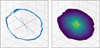 |
Fig. 4. Illustration of the ‘local’ and ‘inner’ choice of PCA integration domain (Eq. (2)), for the simulated relaxed cluster CL6. Left: slicing through a thin gas density layer. Right: slicing through the density distribution enclosed by the same layer. The three lines illustrate the directions of the three principal axes. |
In order to derive triaxial profiles of the shape parameters and the cluster orientation, we introduce the generalised ellipsoidal radius, which is updated with the information on the cluster shape as defined by Dubinski & Carlberg (1991):
 (5)
(5)
where q := b/a and s = c/a ≤ q are the principal axes ratios and the tilde denotes coordinates rotated into the principal-axis frame of the mass tensor. We note that for a = b = c, this definition reduces to the concentric radius  . All profiles shown in this paper are displayed as a function of the generalised ellipsoidal radius. In addition to the quantities we introduced so far, we define the parameter
 (6)
(6)
specifying the relative angle between the major axis at the current radius r and the median major axis orientation of the cluster as a ‘fiducial’ axis. This allows us to quantify the radial variation of orientation in a direction- and coordinate-independent fashion, adapting to the clusters’ own average principal frames. By quantifying and comparing the change in orientation in the principal axis between different methods or data sets, we can investigate the degree of sensitivity of the latter to fluctuations in the isodensity or isopotential shells perturbing the principal axis directions.
3. Results: 3D morphologies of galaxy clusters
We apply the PCA methods defined in Sect. 2 to the gas density and potential distributions of the 85 OMEGA500 clusters. For the gas density, we study the 2S, 3S, 3.5S, and 4S data sets in the variants (a) and (b) discussed in Sect. 2.3. For the potential, we distinguish between variants (i) and (ii) discussed in Sect. 2.2. For each data set, we compute the triaxial ellipsoidal profiles of the quantities ϵ, A and Δϕ (see Eqs. (3), (4), and (6)) averaged over all clusters of the relaxed and non-relaxed cluster subsamples. These profiles are normalised by the halo virial radii r200 and then represented by the median among the cluster population5. We also compute the quartiles of the sample to measure the scatter of each quantity. We start by focusing on relaxed clusters as our main sample of study in Sect. 3.1. We then extend our analysis to the non-relaxed cluster population in Sect. 3.2.
3.1. Cluster shapes from relaxed galaxy clusters
We begin our analysis by determining the ellipticity ϵ(r), the aspheroidicity A(r), and the major axis deviation  of the gas density layers, as defined in Sect. 2.3, for the different data-sets defined in Sect. 2.2. We begin by performing our analysis for the reference configuration 3.5S in the ‘threshold’ filling method b. For this data set, we investigate the cluster shape parameters and their radial behaviour for the gas density both for the inner and the local integration domains. We then compare the results for variations in the parameters of our methods in order to study how the outcome depends on these parameters. In particular, we compare the results for 2S, 3S, 4S for methods (a) and (b), and when using different domains (inner vs. local). This allows us to probe sources of uncertainty but also to study the impact of substructures and their removal.
3.1.1. Cluster shapes from the gas density for the default substructure method (3.5S)
For our reference data set 3.5S, we determine the median cluster shape parameters ϵ, A and Δϕ and their quartiles, which yields the following results for the inner and local domains:
Ellipticity. The ellipticity ϵ of the gas density layers is shown in Fig. 5a. Its median decreases from values of ϵ ∼ 0.75 near the centre down to around ϵ ∼ 0.4 towards the outskirts, regardless of the PCA domain. Around r ∼ r200, the ellipticity ϵ slightly increases again. The quartiles deviate typically by about 20 to 25% (in peaks up to about 50%). The upper quartile shows a larger deviation from the median than the lower quartile. For the inner domain, as expected, the features of the curve are smoothed out and are slightly shifted to higher r due to the delayed response to radial variations that we described in Sect. 2.3. This “lagging” effect can be seen even more clearly when plotting the results for single clusters, as shown for illustration in the example of Fig. 6a.
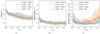 |
Fig. 5. Morphological parameters ϵ(r) (Eq. (3)), A(r) (Eq. (4)) and deviation in orientation Δϕ (Eq. (6)) from the gas density (3.5S) for relaxed clusters. The semi-transparent areas enclose the quartiles of the cluster sample, while ‘med’ and ‘thr’ denote whether regions occupied by substructures are replaced by the median or threshold approach (‘a’ and ‘b’ defined in Sect. 2.2). |
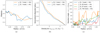 |
Fig. 6. Individual cluster result examples for ϵ(r), r(log10ρ), and Δϕ(r) for the gas density. Left panel: a comparison between inner and local domain for CL1 to illustrate the lagging effect mentioned in Sect. 3.1.1. Middle panel: fluctuation behaviour of the generalised ellipsoidal radius for the same cluster. Right panel: compares the variation in major axis orientation for various different clusters in one particular configuration (local) to highlight the individual fluctuation behaviour in orientation and its differences between the clusters. These figures are intended for illustration only, complementary to our statistical analysis using the full cluster sample. The clusters selected for these figures were picked using a random number generator. The labels ‘med’ and ‘thr’ have the same meaning as in Fig. 5. |
Aspheroidicity. The aspheroidicity profile A(r) is shown in Fig. 5b. Here, we can note that median and quartiles drop by about 60% from values around 0.4 (median), 0.2 (lower quartile), and 0.6 (upper quartile) within the first 10% of r200. This is followed by an almost constant phase in which the median shows a near plateau until r = 0.2 r200 followed by a slight decrease plus fluctuations. The median stays above a value of 0.15 throughout, whereas the quartiles deviate by values of around ∼0.1 from the median and up to ∼0.2 in the peaks (both inner and local). The result for the inner PCA domain differs from that of the local domain mainly in its slightly smoother behaviour, the aforementioned lagging effect, and lower values of the upper quartiles.
Relative orientation. The relative angle  between the major axis at radius r and the median cluster major axis, shown in Fig. 5c, fluctuates very strongly between 5° and 30° in the quartiles (median: ∼11°) between 0 < r/r200 ≲ 0.5 and increases by up to a factor of two towards the virial radius for the local domain. For the inner domain, the orientation is more stable, fluctuating by around 10% and increasing less steeply with radius as a result of the lagging effect. The quartiles on the other hand still show a large spread, with a typical inter-quartile distance of between 10° and 20°.
A look at the same diagrams for examples of randomly picked individual clusters, for example Fig. 6c, shows that radial fluctuations between layers are typically high, with rapid jumps by several tens of degrees occurring between some layers. Investigation of the individual gas density data shows that these rapid changes in orientation are caused by intrinsic fluctuations in the density. For example, for CL25 shown in Fig. 6c, residual fluctuations perturb the shape of isocontours, which are rather close to sphericity at several radii (e.g. ϵρg ∼ 0.2 to 0.4 for this cluster in the outskirts) such that the orientation of the major axis becomes unstable. On top of these fluctuations, as we see in Fig. 6c, there is a monotonic trend of increasing deviation angle with radius. We find that this is a property shared by many clusters and results from perturbations and asymmetries in the gas density distribution increasing with radius. An example of this is CL27, for which the isocontours become elongated and seemingly disturbed in the outskirts. In summary, these various radial variations in the orientations of clusters contribute substantially to the size of the inter-quartile range of Fig. 5c.
3.1.2. Cluster shapes from the gas density for different data sets: Raw, 2S, 3S, 4S
We now extend our analysis to data sets produced for different substructure-removal methods in order to explore how sensitive the derived cluster shape parameters are to the cut-off threshold X. In order to show how important it is to mask substructures in the first place, we also include the original non-processed (‘raw’) density distribution in our comparison. We note that the impact of substructures is even more important when deriving shape information from X-ray data, given the squared dependence of the emissivity on the density. In the following, we present the outcome for these different data sets, which is shown in Figs. 7a,b, and compare to the reference data set:
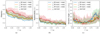 |
Fig. 7. Comparison between substructure-affected (raw) and various cleaned data sets using different cut parameters (2S, 3S and 4S) for a fixed configuration (e.g. local domain + median method). The semi-transparent areas enclose the quartiles of the cluster sample, shown here only for the raw and the 4S results to avoid a crowded plot. Here, ‘med’ has the same meaning as in Fig. 5. |
Raw data set. If the spurious signal from non-virialised substructures is not removed, the axis lengths deviate considerably from each other; for example, for the ellipticity and the aspheroidicity, the median curves deviate from each other by around 20 to 30% below r ∼ 0.75 r200, while the deviation is smaller at large radii. The inter-quartile range increases dramatically, for example enclosing values from ϵ ∼ 0.4 to ϵ ∼ 0.9 for the ellipticity. In contrast, the fluctuations in orientation show opposite trends at small and large radii: Up to r/r200 ≲ 0.4, the raw, non-processed data lead to slightly higher fluctuations than the substructure-cleaned data sets, as can be seen from the median and the upper quartiles. In the outskirts, r/r200 ≳ 0.75, on the other hand, the trend is opposite: here, the median and the upper quartile are similar or lower than for the substructure-cleaned data sets. This suggests that for lower and intermediate radii, the substructures identified by the X-σ criterion introduce significant deviations from the median cluster orientation; while at large radii, conversely, substructure removal increases the deviation. The median orientation itself differs little between the raw and substructure-cleaned data sets, typically by orders of a few degrees only. Thus, the visible deviations between the data sets are mostly showing local deviations between the major axis orientations. In the outskirts, these deviations are the result of a combination of low ellipticity of cluster shapes and residual fluctuations in the gas density that weigh more in the PCA once the largest inhomogeneities caused by substructures have been removed. Contrary to intuition, the asymmetries introduced by these larger inhomogeneities lead to a more stable PCA near the virial radius by defining preferred directions of elongation. However, these are nonetheless strongly misaligned from the median cluster orientation (on average by 20° to 30°) and might not reflect the actual bulk orientation.
Substructure-cleaned data sets. Comparing the outcome for different values of X, we note interesting differences between 2S, 3S, and 4S. While the qualitative trends in the radial evolution are mostly the same, the magnitudes of ϵ, A and Δϕ differ for each choice of X. This can be seen most prominently for the ellipticity, where the 2S curve lies significantly below the 3S result; for example, the median deviates by typically 8% from 3S (and 14% from 4S). For the aspheroidicity and the relative orientation, differences are smaller (around 4% difference between the median values between 2S and 3S, and 10% between 2S and 4S). Thus, the X = 2 criterion in particular leads to more spherical cluster shapes by removing elongation in the direction of the major axis while affecting the two minor axes to a lesser extent. The small differences between 3S and 4S in combination with the large difference between 2S and all the other data sets at large radii suggest that X = 2 is likely too strict, erasing parts of the bulk component both at small and large radii, which is undesired and must be avoided.
We note a low deviation between all data sets at large radii (r/r200 ≳ 0.8) except for the large deviation of 2S from the other curves. The low differences even between 4S and the raw data set suggest that X ≳ 3 may not be efficient for removing all substructures at these radii. Indeed, when inspecting the isocontours of the substructure-cleaned gas-density data sets, we note that a weak impact of inhomogeneities is still present and perturbs the shape of the gas-density distribution.
3.1.3. Cluster shapes from the gravitational potential
For the gravitational potential, we distinguish two different data sets: The non-processed (“raw”) simulation output and a pre-processed data set in which regions occupied by gas substructures (identified with X = 3.5) are substituted by the median potential in shells in formal analogy to the procedure for the gas density. With the raw version, our aim is to compare whether the true, non-processed potential, including all its intrinsic asymmetries and contributions from subclumps, still allows for a less ambiguous shape determination than the substructure-removed gas density. The second data set, produced by substituting the median potential in substructure regions, is included to provide a slightly different comparison that aims to compare the data sets pre-processed in the most similar way. The results are shown for the local PCA method in Fig. 8 next to the results for the gas density, which are shown for a direct comparison. We summarise and compare the results below.
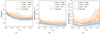 |
Fig. 8. Gas vs. potential in terms of morphological parameters ϵ(r) and A(r), and deviation in orientation Δϕ from the gravitational potential for relaxed clusters, and comparison to the gas density. The semi-transparent areas enclose the quartiles of the cluster sample, while ‘med’ and ‘thr’ denote whether regions occupied by substructures are replaced by the median or threshold approach (‘a’, ‘b’, and ‘ii’ defined in Sect. 2.2). The label ‘raw’ denotes the non-processed original data set. |
Ellipticity. The gravitational potential Φ (see Fig. 8a) starts at a median ellipticity of ϵΦ ∼ 0.6 in the core, which decreases down to a near plateau at ϵΦ ∼ 0.4 towards r/r200 ≳ 0.5. Thus, its behaviour is qualitatively similar to that of the gas density, except that ϵΦ is consistently smoother, slightly rounder than the gas (with a median ellipticity of about 15% to 20% lower), and has a much narrower inter-quartile range (by factors ≳2). Thus, at fixed radius, the spread in ϵΦ over the cluster population is considerably smaller than for the gas density. These results are quite insensitive to the PCA domain and hold even when comparing the local potential data set with the substructure-removed inner gas data set. We note that when comparing individual clusters, the difference in fluctuation behaviour between gas and potential data sets becomes even larger because the sample averaging itself smoothes out many of the fluctuations in ϵρg that contribute to the large inter-quartile distances. For illustration, see the example in Fig. 9a in comparison to Fig. 6a. Moreover, we note that ϵΦ is nearly insensitive to whether or not we mask regions containing substructures. Thus, the shape of the potential along its major axis is highly stable against local fluctuations in the data set. Another interesting difference between ϵΦ and ϵρg is that the potential curve remains flat around r200 while the gas density ellipticity shows a slight increase due to growing asymmetries in the gas density distribution towards r200.
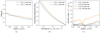 |
Fig. 9. Individual cluster result examples for the gravitational potential, showing the same random set of clusters as we used in Fig. 6. These figures are intended for a better illustration only, complementary to our statistical analysis using the full cluster sample. The label ‘raw’ refers to the non-processed original potential data set. |
Aspheroidicity. From Fig. 8b we can see that the gravitational potential is considerably closer to spheroidal symmetry than the gas density, with values of the average gas density for A being twice as high as the potential. While for the gas density the median aspheroidicity starts from a central value slightly above 0.4 and mostly remains fluctuating around 0.2 to 0.25 with higher radius, regardless of the method, the median aspheroidicity for both potential data sets starts slightly above 0.2 and decreases very smoothly below 0.1 until r ∼ 0.9 r200. In comparison to the gas density, A(r) changes much more slowly with radius and with less fluctuation, and again the inter-quartile range is much narrower. The upper quartile of AΦ mostly remains even below the median ϵρg or just touches it. Differences between the median-substituted and the raw potential data sets are again typically very small, in contrast to the huge difference we note between the 3S (or 4S) and raw gas density data sets in Fig. 7b.
Relative orientation. The spatial orientation of the major axis computed from the potential shows considerably less fluctuation and deviation from the median orientation than for the gas density data set. The angular difference Δϕ to the median cluster major axis mostly remains below 10° (median difference: 5°), while for the gas density it varies between 10° and 30° (median difference: 14°). The upper quartile for the potential varies between values of 10° and 20° (gas density: 20° to 60°). The upper quartile is slightly lower as well, staying mostly below 50° for the potential while the relative deviation from the median is typically around 40% higher for the gas density. For the inner gas density data set, the deviation angle is mostly similar to that of the local method; however, towards large radii, r ≳ 0.7 r200, the deviation angle for the inner gas density data set is similar to that of the potential data sets because of the slow response of the so-defined mass tensor to local shape changes. Still, the corresponding value for the inner potential data set is considerably lower. Thus, comparing only the inner, median-substituted data sets for gas and potential, the potential shows a more stable deviation angle at a smaller value than for the gas density.
3.2. Cluster shapes of non-relaxed clusters
We now turn to the 53 non-relaxed clusters of the OMEGA500 simulation to study their shapes and investigate the influence of the cluster’s dynamical state by comparison with the relaxed sample. The non-relaxed cluster sample consists of objects showing signs of recent dynamical activity, such as irregular X-ray isophotes, as defined through the SPA criteria in Sect. 2.1. For the shape parameters that we derive for the 3D matter and potential distributions, this may imply asymmetries, multiple mass peaks, and higher deviations between gas and potential isosurfaces. Due to the larger irregularity, the prevalence of substructures matching the X-σ criterion is higher as well, such that the uncertainties and ambiguities related to substructures that we identified in the previous section might become even more important. In this section, we fix the substructure criterion to the default choice of X = 3.5 to focus on the impact of the cluster dynamical state by comparing the results for the relaxed and non-relaxed samples.
Ellipticity. The ellipticity profile presented in Fig. 10a shows that the gas density ellipticity ϵρg is consistently higher than the gas density ellipticity in the relaxed sample by around 15%. The inter-quartile distance also increases. For the potential, the median ellipticity ϵΦ is very close to its relaxed values, with the difference that it decreases more slowly with radius than for the relaxed sample, until it reaches the same plateau at r/r200 ≳ 0.75 as before. However, interestingly, the inter-quartile distances are comparably large for the potential, with a pronounced peak in the upper quartile at r/r200 ∼ 0.15, touching the upper quartile of the gas density ellipticity. We note that in this region, the impact of the presence of multiple cluster cores appears to be largest, giving rise to a bi- or multimodality in the distributions of gas and dark matter, while causing equipotential surfaces to become at least more elliptical (for two examples, see Fig. 11) raises the upper quartile of both gas density and potential ellipticities considerably.
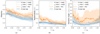 |
Fig. 10. Morphological parameters and deviation in spatial orientation for non-relaxed clusters, comparing gas density and potential. The semi-transparent areas enclose the quartiles of the cluster sample, while ‘med’ and ‘thr’ denote whether regions occupied by substructures are replaced by the median or threshold approach (‘a’ and ‘b’ defined in Sect. 2.2). The label ‘raw’ denotes the non-processed original data set. |
Aspheroidicity. For the aspheroidicity shown in Fig. 10b, one can make an interesting observation: the median value for the potential increases only slightly compared to the relaxed sample, staying below 25%, whereas for the gas density, Aρg increases to values of between 30% and 55%, with broad quartiles and strong fluctuations, while the potential is comparably smooth and nearly constant in AΦ throughout large intervals in radii.
Spatial orientation. The change in spatial orientation of the major axis is shown in Fig. 10c. Here, we can see a rather drastic increase and strong fluctuations in the results for the gas density, fluctuating between 30° and 40° in the median, with upper quartiles extending beyond 60° over a large range in radii. The potential, in contrast, still remains much more stable in its spatial orientation, with median values of between 5° and 18° and upper quartiles up to about 30° – even though in comparison to the relaxed case, the level of potential fluctuations has increased very slightly.
4. Discussion
In the following, we discuss the outcomes of our morphological analyses as well as their implications and uncertainties. We comment on the physical implications of our results and on explanations for them, and discuss methodological aspects that lead to differences or ambiguities in the outcome. We start by discussing common trends that were visible in all data sets and then focus on the differences between single methods. The latter we discuss in the context of removal of substructures, the impact of our choice of PCA method, and the influence of the clusters’ dynamical state, which reflects in the difference between the relaxed and non-relaxed populations.
4.1. Physical context and implications of cluster shapes
We find in this study that relaxed clusters have a median ellipticity of ⟨ϵρg⟩∼0.5 ± 0.1 (for the gas density shells) and ⟨ϵΦ⟩∼0.38 ± 0.06 (for the potential), when averaged within the interval r ∈ [0, r200]. The deviation from spheroidal symmetry was quantified as ⟨Aρg⟩∼0.21 ± 0.08 and ⟨AΦ⟩∼0.11 ± 0.06. Thus, the gas density shows a deviation from spheroidicity that is on average twice that shown by the potential. These values are consistent with the perturbative triaxial modelling of halo potentials by Lee & Suto (2003), who found an analytic relation between gas density and mass axis ratios that allows to arrive at gas ellipticities of order 0.2 to 0.5; and at small values of the aspheroidicity of below 0.2. Our results for the potential shape parameters are in good agreement with those obtained from N-body simulated haloes by Hayashi et al. (2007), who suggest ϵΦ ∼ 0.48 ± 0.06 near the halo centre and less at higher radii; and with AΦ ∼ 0.13 ± 0.02 remaining almost constant over a large range in radius. An earlier systematic study of 16 clusters simulated with the ART code by Lau et al. (2011) shows very similar values for both quantities in the non-radiative runs: ϵρg ∼ 0.4…0.6, ϵΦ ∼ 0.5…0.6, Aρg ∼ 0.2…0.4, and AΦ ∼ 0.2…0.3. Surprisingly, in the study by these latter authors, the potential has a partially higher ellipticity than the gas density and ϵΦ increases again after r/r200 ∼ 0.3, although the uncertainties are significant. Finally, our gas ellipticity measurements are consistent with those obtained earlier for a sample of 80 OMEGA500 clusters by Chen et al. (2019), who focused on the gas ellipticities and their correlation with mass accretion history, finding values for ⟨ϵρg⟩ peaking around 0.6, with scatter of between 0.3 and 0.8.
One of the main trends we are able to identify in the morphological evolution of all data sets is that of an overall decrease in ellipticity and aspheroidicity of both gas and potential with radius. Our study suggests that clusters become rounder and also more spheroidal with increasing radius, in agreement with earlier theoretical studies (e.g. Hayashi et al. 2007; Lau et al. 2011). Although in all comparisons, we find the gravitational potential to be more symmetric than the gas density at most radii, the qualitative behaviour of ellipticity, aspheroidicity, and major axis deviation is mostly very similar between gas and potential. Quantitatively, differences can be noted in the (consistently) larger fluctuations and larger asymmetries present in the gas density distribution. These differences are notable for all substructure-cleaned data sets and become much larger when not removing substructures in the first place.
The trend of isocontours becoming more spherical with growing radii is expected for a gravitational potential generated by an ellipsoidal mass distribution. From potential theory, it is well known that the exterior equipotential surfaces of thin homoeoids are confocal spheroids (Binney & Tremaine 2008) and that the monopole contribution dominates at large distances from a centrally concentrated mass distribution6. In addition, earlier works suggested that the shapes of cluster mass distributions themselves become slightly rounder towards the outskirts in numerical N-body simulations (e.g. Allgood et al. 2006; Vera-Ciro et al. 2011, and references therein). For the intracluster gas residing in a potential well generated by an arbitrary mass distribution, we expect the gas density distribution to follow the potential closely in regions that are in approximate hydrostatic equilibrium. The hydrostatic equation implies the gradients of gas density and potential to be parallel, ∇ρgas × ∇Φ = 0, such that equipotential surfaces are common isosurfaces of density, pressure, and X-ray emissivity (e.g. Buote & Canizares 1994). Thus, we expect the gas density to follow similar overall trends in orientation and axis ratios to the potential.
Nonetheless, the parameters characterising potential shapes are neither found nor expected to be in full agreement with those of the gas density (see e.g. Figs. 8 and 10). Even in ideal hydrostatic equilibrium, the gravitational potential Φ is expected to be distributed more smoothly than the gas density ρg. This can be seen explicitly for an ideal or polytropic gas with an effective adiabatic index γ, for which the hydrostatic equation implies the following analytical relation (Konrad et al. 2013):
 (7)
(7)
For realistic adiabatic indices, 1.1 ≲ γ ≲ 1.2 (Finoguenov et al. 2001), the small exponent causes potential fluctuations to be suppressed relative to density fluctuations by factors of between 5 and 10:
 (8)
(8)
This leads to a smoothing that can be compared to a low-pass filter suppressing small-scale components in the potential distribution, which therefore weigh less in the mass tensor.
However, the gas density contains significant fluctuations even for relaxed clusters and after excluding substructures with the advanced methods such as the X-σ criterion. Some of these fluctuations are consequences of small deviations from the hydrostatic assumption. Due to the large typical dynamical and thermal timescales of galaxy clusters in comparison with the age of the Universe, hydrostatic equilibrium in galaxy clusters is only approximate. With a free-fall timescale similar to that of sound crossing, the intracluster medium can be trans-sonic over large regions, causing slight shocks across the cluster that lead to discontinuities in the density. The presence of such bulk fluctuations is expected to depend only slightly on the input gas physics (Zhuravleva et al. 2013; Roncarelli et al. 2013). At the same time, further deviations from hydrostatic equilibrium are expected due to dynamical activity (i.e. accretion and merging activity of substructures) at the outskirts, r ≳ r500. In the cluster core regions, moreover, the effects of radiative cooling and baryonic feedback – not included in this simulation – may affect the shapes of clusters, with radiative cooling in the centres expected to lead to a more spherical gravitational potential due to a more centrally condensed mass distribution (e.g. Dubinski 1994; Kazantzidis et al. 2004), while at the same time, AGN feedback may largely counteract this effect by preventing the gas from cooling (Bryan et al. 2013; Suto et al. 2017; Chua et al. 2019). Still, the details of these mechanisms need to be better explored and understood. When reconstructing cluster shapes in practice, we expect that deviations from the assumption of hydrostatic equilibrium may be a larger source of concern than the impact of input gas physics on the actual shapes within the inner cluster region.
4.2. Impact of dynamical state
For the non-relaxed cluster sample, we note that clusters have both more elliptical and more triaxial shapes, especially when looking at the gas density distribution. In addition, we find slightly larger quantitative differences between gas and potential (see e.g. Fig. 10), as is to be expected given that the clusters are dynamically more active as indicated by their irregular X-ray morphologies. In such cases, large parts of the gas may not yet have settled into approximate hydrostatic equilibrium, leading to more pronounced clumpiness, shocks, and asymmetries. The presence of two or multiple merging cores can, in addition, lead to more elliptical potential isosurfaces; two examples of this are shown in Fig. 11. The increased ratio of ellipticity to aspheroidicity of the potential suggests that a large number of mergers have their mass centres separated along (or near) the major axis. This is consistent with the predictions of gravitational collapse of dark matter driven by self-gravity for an initial Gaussian random field, which implies that cluster haloes are elongated along the direction of their most recent major mergers because of the anisotropic accretion and merging along filamentary structures (e.g. Limousin et al. 2013). The implication for the ellipticity of the potential becomes apparent from Fig. 10a, where we see increased upper quartiles for the potential, although the latter is still very smooth and deviates significantly less from spheroidal symmetry than those of the gas density.
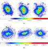 |
Fig. 11. Potential isocontours overlaid on 2D projections of the dark matter distribution for two non-relaxed clusters showing bi- or multimodality in their mass distribution. The three panels in each case show projections of the simulated data cube for the three spatial orientations x, y, and z of the cube. (a) Cluster CL10. (b) Cluster CL77. |
4.3. Impact of methods and data sets
In the previous section, we discuss the impact of density inhomogeneities on the gas density. The presence of inhomogeneities and asymmetry, whether caused by non-virialised subhaloes or residual shocks in the bulk gas component, complicates the determination of cluster shapes by introducing ambiguities and uncertainties, which have a much smaller effect on the gravitational potential. Apart from these difficulties when using the gas density, the 3D morphology of clusters can be defined in several different ways that may be ambiguous with respect to the choice of defining isodensity bins, summation volumes, and radial profiles.
4.3.1. Substructures and their removal
Substructures are density inhomogeneities that are not virialised with the cluster and therefore need to be identified and removed prior to estimating the hydrostatic mass (or potential) based on the gas density distribution (e.g. Nagai & Lau 2011; Zhuravleva et al. 2013; Roncarelli et al. 2013; Vazza et al. 2013, see also our companion paper Tchernin et al. 2020). Additional analysis based on the abundance and/or temperature of these clumps could be used to distinguish the substructures from the cluster body. However, such information is not always available as it requires high-resolution measurements. Nowadays, there exist several different ways to identify or suppress substructures. For example, Dubinski & Carlberg (1991) applied an r−2 weighting in the mass tensor to suppress the impact of dark matter subclumps, which are most prevalent in the dynamically younger cluster outskirts; however, see Zemp et al. (2011), who suggested that this introduces systematic biases. Another definition of substructures is based on the (residual) gas clumpiness factor ρ2/ρ (e.g. Roncarelli et al. 2013, and references therein) or uses the more advanced X-σ criterion (with X = 3.5, e.g. Zhuravleva et al. 2013; Lau et al. 2015), which takes into account the lognormal shape of the bulk gas distribution. Nevertheless, applying such methods may alter the intrinsic shape of the cluster, which is the information we actually want to extract.
We therefore investigated the systematic effect coming from such a treatment of data on the outcome of the shape reconstruction. For this we compared several different generalisations of the 3.5σ method, which we dubbed the X-σ method: Apart from the X = 3.5 criterion, we produced versions of the gas density data set for X = 2, X = 3, and X = 4 as well as for the raw, non-processed gas density distribution to highlight the effect of substructure removal on the final results. It should be noted that the choice for the cut-off parameter X is fully arbitrary and needs to be chosen carefully to avoid erasing too much of the bulk component.
This introduces two notable sources of ambiguity: (1) the value that should be chosen for X is unclear, because there is neither a sharp distinction between bulk and substructure X-ray signals nor a way to distinguish whether asymmetries in the density isolayers are caused by substructures or are intrinsic to the bulk (triaxiality–substructure degeneracy). (2) What to substitute for the regions occupied by substructures it is also unclear. Even after cleaning substructures, we are left with residual fluctuations in the bulk component, for example due to small shocks present in the gas. These fluctuations are present on all scales and affect observable quantities like the X-ray emission, which depends on the square of the gas density. In contrast to the decreasing ellipticity and aspheroidicity, we observe that the relative deviation in orientation of the major axis generally increases with radius. This is most likely the result of two combined effects: First of all, substructures become important at large radii, affecting the derived shape parameters. Second, the more spherical the intrinsic cluster shape is, the less well the orientation of the three axes is constrained and the more sensitive it becomes to any fluctuations along the contours of the ellipsoid. This phenomenon, which is illustrated in Fig. 12, affects the stability of the PCA.
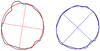 |
Fig. 12. Illustration of the effect of fluctuations on the principal axis of a density isocontour. This example shows isocontours taken from the 3S (left) and 2S (right) data sets of a relaxed cluster when computing a slice of the cube. |
This is a problem that does not affect the gravitational potential, which we find to be almost insensitive to the contributions of subclumps; this enables the use of the raw, non-processed potential data for the shape determination without any problems. Due to its suppression of small-scale components, the potential distribution is intrinsically smoother and more symmetric than the gas density.
4.3.2. PCA domain
We applied the PCA method to simulated clusters for different definitions of the integration domain for the mass tensor (‘inner’ vs. ‘local’; see Fig. 4). We notice that information derived from the local domain is more sensitive to fluctuations in the gas density, as it responds to any local changes in the shape of isocontours. The inner domain, in contrast, provides a more robust dataset, as it consists of a sum of contributions over larger regions enclosed by the isocontours. This suppresses spurious small-scale fluctuations, but it can also result in possibly intrinsic features being hidden or distorted, because the mass tensor computed in the inner domain responds slowly to the radial evolution of cluster shapes. This can be noted especially at higher radii, where the radial profiles of shape quantities no longer reflect the local shape of cluster shells but rather the average behaviour of interior shells. Similar observations were made by Zemp et al. (2011), who studied different choices of defining a halo shape tensor. A related problem is the non-trivial dependence of quantities derived from the inner domain on the slope of the gas density profile. The latter modifies the effective weight of single pixels, increasing it towards high-density regions. As the slope can vary between clusters, this further complicates the interpretation and comparison of profiles between different clusters. In our study, we see that the differences between the two methods are particularly large for the gas density at large radii. Here, the absolute level of fluctuation and uncertainty in ellipticity, aspheroidicity, and orientation angle is considerably larger for the local method. In contrast, the difference between the two domains is found to be remarkably small for the gravitational potential. Thus, the potential-based PCA is much more robust against the domain definition than the gas-based shape reconstruction.
4.3.3. Uncertainties due to bin and radius definition
The radial evolution of shape quantities depends only weakly on the choice of bin width. We explored the impact of the bin width on our results by comparing different choices for the logarithmic bin width parameter. An example is shown for illustration in Fig. 13, where we can see that even a bin width of twice the size causes fluctuations of the quartiles in the orientation angle that are still of similar size to or slightly below the original value. In contrast, the aspheroidicity does not change significantly except for the innermost radii. Our tests using different bin width parameters suggest that a large part of the fluctuations we find in the parameters characterising the shape and orientation of the gas density distribution are not caused by an overly narrow bin width.
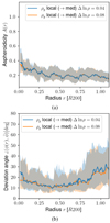 |
Fig. 13. Impact of bin width on shape parameters quantifying asymmetry and orientation. The label ‘med’ denotes that regions occupied by substructures are replaced by the median (‘a’ is defined in Sect. 2.2). |
The noisy fluctuations present in the radial evolution of the major axis orientation of the gas density lead us to question whether these fluctuations are entirely intrinsic or might be affected in part by the definition of the generalised ellipsoidal radius r. The latter is sensitive to fluctuations in the axis ratios, which in principle can lead to small random displacements of the plotted quantities along the r-axis. In order to quantify how stable the ellipsoidal radius is with respect to axis ratio fluctuations both with radius and between different clusters, we investigate the behaviour of the radius r as a function of the density bin for the individual cluster data sets. We find that the resulting curves r(log10ρ) are in all cases rather smooth. An example is shown for illustration in Figs. 6b and 9b. This suggests that the effect that intrinsic fluctuations of iscontours have on the generalised ellipsoidal radius r are small, and are not significant enough to cause artificial fluctuations in ϵ(r), A(r), or  purely because of random shifts along the r-axis. However, we note that radial fluctuations in ϵ(r) and A(r) are naturally connected to changes in the axis orientations; for example, small random fluctuations in the axis directions might be visible in the length ratios too. Nevertheless, these should, to a large extent, average out when taking the sample median. Still, as Figs. 5c, 6c, and 10c show, the large fluctuations indicating instabilities in the PCA are potentially problematic for measuring the shape of the gas density distribution. The values for ϵρg and Aρg may therefore be affected by larger uncertainties than indicated by the quartiles only. This problem does not significantly affect the potential, whose orientation is highly stable for the case of most clusters.
4.4. Importance of accurate shape assumptions
In the context of our comparisons between the symmetries of gas and gravitational potential, we note that it is crucial to model the 3D shape of a cluster as correctly as possible when working with quantities like the gas density or the X-ray emissivity. However, this is not trivial, even for the most relaxed clusters, as our results show. However, we find that even small variations in ellipticity can lead to significant errors in the resulting triaxial profile. To illustrate this point for an example, we extracted a triaxial profile of the X-ray emissivity for the cluster CL135 whose mass and potential profiles we studied in detail in Tchernin et al. (2020), assuming three different values for the ellipticity: the optimal ellipticity obtained for CL135 from our PCA in the range [0.5; 1] r500: ϵ = 0.36; the optimal ellipticity for radii larger than r500: ϵ = 0.2; and the spherical assumption: ϵ = 0 (see Fig. 14). As we can see, a small variation of the ellipticity (between 0.2 and 0.36) leads to an average deviation of about 25% over the entire cluster radius range. Moreover, assuming spherical symmetry for a cluster with an ellipticity as low as 0.36 (in the range [0.5; 1] r500) and 0.2 (in the outskirts) can lead to underestimation of the X-ray emissivity profile by up to 50% in the region between r500 and r200, and by 30% between [0.5; 1] r500, which is part of the region accessible to X-ray measurements. This effect can have non-negligible consequences on the study performed with these profiles (e.g. in HE mass estimates).
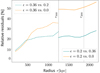 |
Fig. 14. Relative residuals in X-ray emissivity profile for the relaxed simulated cluster CL135 studied by Tchernin et al. (2020), for the region [0.5, 1] r500 (ϵ ≈ 0.36), compared to the optimal ellipticity in the region [r500, r200] (ϵ ≈ 0.2). These optimal ellipticity values are obtained using the inner domain. For comparison, the relative residuals with respect to the spherical symmetry assumption are also shown. Here, x versus y means: |x−y|/x, with x and y being the triaxial profiles derived for a given ellipticity. The vertical lines indicate r500 and r200, respectively. |
Similar impacts due to over-simplified cluster shapes are expected to be numerous, even though they are difficult to quantify given that the actual shapes of clusters are unknown. For example, using a technique like the median approach (Eckert et al. 2015) to remove substructures in spherical shells in a spheroidal cluster can lead to underestimation of the resulting profile by up to 15% (see Figs. A.2a and A.8 in Tchernin et al. 2020).
5. Summary and conclusions
The 3D structure of galaxy clusters contains important information on the initial density field, the halo assembly, cosmological parameters, and the nature of dark matter and gravity. As such, it will play a crucial role in upcoming cosmological studies. Information on the gas density distribution obtained from X-ray and tSZ observations has been extensively used to draw cosmological constraints. However, we see that deriving the shape of a galaxy cluster is not trivial even for a relaxed cluster for which we have all the simulated data at hand. Based on the gas density distribution of relaxed simulated galaxy clusters, we emphasise that deriving the shape of a galaxy cluster is not trivial even from a full 3D simulation. This is due to the fact that cluster shapes evolve with time and therefore their morphology can vary with the distance to the centre. The presence of substructures adds to the complexity of the problem, as their exclusion introduces new uncertainties and ambiguities; for example, using an overly strict criterion may alter the reconstructed shape of a cluster.
In the present study, we analysed the shapes of 85 relaxed and non-relaxed clusters of galaxies from the OMEGA500 simulation. We highlight the difficulty in removing substructures from the matter density distribution and show how this affects the reconstructed shape of the cluster estimated from the mass tensor. We also illustrate the consequences an incorrect assumption on the cluster shape can have on the resulting extracted X-ray emissivity profiles derived for a low-ellipticity relaxed cluster. As a result, we arrive at two main conclusions, which we summarise in the following two subsections.
5.1. Shortcomings of the gas density as a shape proxy
Our results show that the distribution of gas density in clusters of galaxies is a weak proxy for cluster shape. This is because of large inhomogeneities in gas density due to substructures, which need to be excluded and are partially degenerate with the triaxiality of the cluster. In addition, different methods exist both for identifying and removing substructures. Even when substructures are excluded, fluctuations in the bulk gas density complicate the morphological analysis. We tested here: (1) how the result of the PCA is affected by the method used to remove substructures; (2) the sensitivity of the PCA to perturbations in the resulting isodensity shells quantified by the radial fluctuation behaviour; (3) how the PCA domain (‘inner’ vs. ‘local’ domain) influences the outcome of the cluster shape determination; and (4) by how much the cluster shape parameters and orientation vary between different clusters.
Clusters are often assumed to have a simple geometric shape (spherical or spheroidal) when extracting various types of information from 2D observations and linking these to theoretical models. The shape of the gas density distribution is more difficult to characterise using a simple model, deviating strongly from spherical symmetry ⟨ϵρg⟩∼0.5 and significantly from spheroidicity ⟨A⟩∼0.21. Given the intrinsic asymmetries and inhomogeneities in the gas density even after removing substructures, not only does the use of spheroidal models lead to a loss of information, but in addition the gas density distribution allows for a less stable PCA. Both the shape and the orientation of isodensity shells measured for the gas density distribution vary significantly with radius, analysis method, substructure-cleaning method, dynamical state, and between different clusters. For example, the PCA applied to data cleaned from substructures with the 3.5σ criterion leads to large deviations both between different clusters and with respect to other choices of the substructure-identification parameter X. In addition, shape quantities derived from the mass tensor are subject to significant fluctuations with radius, for example in the orientation angle. Therefore, studies of cluster shapes based on the gas distribution in galaxy clusters are not robust.
We also highlight that it is crucial to properly approximate the 3D shape of a cluster when dealing with quantities such as the gas density or the X-ray emissivity. Even small variations in ellipticity can lead to significant errors in the resulting triaxial profile (see Fig. 14). In addition, we observe in our companion paper (Tchernin et al. 2020) that using a technique such as the median approach (Eckert et al. 2015) to remove substructures in spherical shells on a spheroidal cluster can bias low the resulting profiles. This implies that systematical errors arising from substructure removal should be taken into account in the extracted X-ray profiles. Such systematic errors will propagate into other quantities derived from these profiles; for example into HE mass estimates.
5.2. Advantages of using the gravitational potential
The gravitational potential is in multiple ways better suited as a shape and profile reconstruction quantity than the gas density. Not only does it enable a simpler, less ambiguous definition compared to cluster masses (given its nature as a local quantity directly related to observables, e.g. Angrick & Bartelmann 2009; Lau 2011; Angrick et al. 2015) and lower systematic errors in profile reconstructions on simulated data (e.g. 6% bias instead of 13% for the HE mass; and a scatter reduced by ∼35%, see Tchernin et al. 2020), but the results of our study suggest that the shape of the gravitational potential is better approximated by a simple geometry (e.g. spheroidal symmetry) without significant loss of information. We also find that, due to its smoothness7, the potential allows for a more robust PCA, avoiding several problems and ambiguities in determining cluster shapes.
We noted that even for dynamically relaxed clusters in approximate hydrostatic equilibrium, the characterisation of galaxy cluster shapes based on the gravitational potential Φ confers significant advantages over using the gas density. In particular, a simple geometry leads to lower scatter. Indeed, cluster gravitational potentials can be better approximated by a simple spheroidal model, that is, with a typical aspheroidicity ⟨AΦ⟩∼0.11 twice as low as the gas density, a slightly lower ellipticity ⟨ϵΦ⟩∼0.38, and with less scatter (in all quantities) among the relaxed8 cluster population. Studies aiming at reconstructing the potential from observations in order to constrain theoretical predictions are therefore significantly less affected by simplifying assumptions about its shape than when using the gas density. As 2D observations always need to be deprojected to be related to theoretical predictions, this allows for a much more straightforward cluster characterisation. Still, all information about the underlying mass distributions (both gas and dark matter) and on common observables (X-ray, lensing, SZ, galaxy kinematics) are encoded in the gravitational potential (see e.g. Konrad et al. 2013; Sarli et al. 2014; Stock et al. 2015; Majer et al. 2016).
A second advantage of the gravitational potential is its smoothness and stability against fluctuations. As the gravitational potential is considerably smoother than the matter density distribution, its isoshells are nearly unaffected by local perturbations of any kind in the mass distribution, even though it includes the full9 impact of non-virialised substructure contributions δΦ. The spatial orientation of potential isolayers in particular remains highly stable with increasing ellipsoidal radius (ΔϕΦ ∼ 5° to 10° for relaxed clusters). This shows that the cluster orientation is relatively constant with radius; and this needs to be contrasted with the large variations we measure for the gas density (≳10 to 30° and much larger in individual cases). Fluctuations present in the mass density distribution are smoothed out when integrating Poisson’s equation to derive the gravitational potential. The extremely low impact of inhomogeneities on the potential-based PCA implies a more reliable physical characterisation of galaxy clusters, with less uncertainties on shape parameters. In particular, no pre-processing step for substructure removal is needed, which requires additional assumptions. In this context, ambiguities regarding cut thresholds and filling methods are entirely avoided. Thus, the gravitational potential encodes the shape information of the underlying mass distribution in a smooth quantity, which (in projection) can be straightforwardly linked to many different observables.
Finally, these advantages apply to clusters in any dynamical state. Even for non-relaxed clusters, the potential Φ can be approximated by a spheroid with a relative deviation of ≲20% from the actual shape. This result is very encouraging. Combined with the fact that the potential can be relatively well reconstructed for clusters in any dynamical state (with a total bias of 6%, as demonstrated in our companion paper Tchernin et al. 2020), this implies that by characterising galaxy clusters by their gravitational potential in cosmological studies, we can include dynamically active clusters. This will help tighten the existing constraints on the cosmological models. Many cosmological studies rely on relaxed galaxy clusters only (e.g. Vikhlinin et al. 2009; Mantz et al. 2016; Applegate et al. 2016), owing to the fact that these are more easy to compare to theoretical predictions because of their expected spherical (or spheroidal) shapes. However, taking into account dynamically active clusters in such studies will increase the sample statistics. Moreover, as it is generally difficult to assess whether an observed cluster is dynamically active or not, including these clusters will also significantly simplify the process of selecting the clusters. This will be possible by replacing the mass of clusters by their gravitational potential in such studies (see also Lau 2011), both in theoretical predictions (using a ‘potential function’ as e.g. in Angrick et al. 2015) and in observations, where the potential can be reconstructed from direct observables such as lensing, X-ray, or millimetre observations (as done in e.g. Tchernin et al. 2015, 2018; Merten 2016; Huber et al. 2019). The smooth, nearly spheroidal shape of the potential (even for dynamically active clusters) will be an important advantage for this purpose.
Characterising galaxy clusters by their gravitational potential in cosmological studies will allow improvement of constraints on cosmological parameters, the nature of dark matter, dark energy, and gravity. The prospects for releasing the full power of potential-based cluster reconstructions for cosmological studies are highly promising given that large homogeneous and high-quality cluster data sets are or will become available across the electromagnetic spectrum in the near future. X-ray observations such as those from XMM-Newton or Chandra provide high-quality constraints for individual cluster reconstructions (e.g. Merten et al. 2011; Jauzac et al. 2016, 2019; Hallman et al. 2018; Pandge et al. 2019). In combination with other probes, such as gravitational lensing from optical or SZ from millimetre observations from Planck, SPT, ACT, or IRAM for example, these observations can be used in multi-wavelength analyses to probe the physical conditions of clusters out to large radii (e.g. Morandi et al. 2012; Eckert et al. 2017; Ghirardini et al. 2018; Tchernin et al. 2018; Siegel et al. 2018; Huber et al. 2019). The next decade of cluster cosmology will benefit greatly from advanced large-scale surveys such as eROSITA (Merloni et al. 2012), Euclid (Laureijs et al. 2011), and LSST (LSST Science Collaboration 2009), which are going to yield order-of-magnitude increases in cluster samples, thus transforming our our ability to use galaxy clusters as cosmological probes dramatically. It will be highly interesting to see what improvements and new insights can be achieved by using a potential-based modelling approach.
A spheroid is an ellipsoid, whose axis ratio satisfies a > (b = c), where a is the major axis of the ellipsoid and b, c the two minor axes.
While gravitational lensing measurements do not rely on symmetry assumptions, the cluster masses are often estimated using such assumptions.
These are fluctuations not identified and removed by the X-σ criterion either because their amplitude is too weak, or because they belong to the small-scale fluctuations intrinsically present in the bulk component e.g. due to gas motions (see e.g. Zhuravleva et al. 2013).
The definition of M is analogous to the definition of the covariance matrix for a distribution of data points.
We note that we use the median here instead of the mean because it is less sensitive to outliers e.g. caused by largely perturbed individual clusters.
This is valid at least as long as the effects of substructures and – at very large radii – mass contributions from filaments can be assumed to be of negligible order, as is the case for our data sets.
Which results from the suppression of small-scale modes compared to the density distribution (see also Sect. 2 in Tchernin et al. 2020).
For the non-relaxed sample, see the item “dynamical state” below.
Or partial, when masking regions in which gas substructures where identified.
Acknowledgments
We thank the anonymous referee for valuable comments that helped to greatly improve this manuscript. We would like to thank Matteo Maturi, Sara Konrad and Jonas Große Sundrup for stimulating discussions and feedback. This paper was supported in part by the Deutsche Forschungsgemeinschaft under BA 1369/28-1 and by the Swiss National Science Foundation under P2GEP2 159139. Sebastian Stapelberg and Matthias Bartelmann’s work is funded by the Deutsche Forschungsgemeinschaft (DFG, German Research Foundation) under Germany’s Excellence Strategy EXC 2181/1 – 390900948 (the Heidelberg STRUCTURES Excellence Cluster). We thank Daisuke Nagai for kindly giving us the permission to use the data from the Omega500 simulation. The Omega500 simulations were performed and analysed at the HPC cluster Omega at Yale University, supported by the facilities and staff of the Yale Center for Research Computing.
References
- Allgood, B., Flores, R. A., Primack, J. R., et al. 2006, MNRAS, 367, 1781 [NASA ADS] [CrossRef] [Google Scholar]
- Angrick, C., & Bartelmann, M. 2009, A&A, 494, 461 [NASA ADS] [CrossRef] [EDP Sciences] [Google Scholar]
- Angrick, C., Pace, F., Bartelmann, M., & Roncarelli, M. 2015, MNRAS, 454, 1687 [NASA ADS] [CrossRef] [Google Scholar]
- Applegate, D. E., Mantz, A., Allen, S. W., et al. 2016, MNRAS, 457, 1522 [NASA ADS] [CrossRef] [Google Scholar]
- Banerjee, A., Adhikari, S., Dalal, N., More, S., & Kravtsov, A. 2020, JCAP, 2020, 024 [CrossRef] [Google Scholar]
- Bartelmann, M. 2010, Class. Quant. Grav., 27, 233001 [CrossRef] [Google Scholar]
- Bartelmann, M., Limousin, M., Meneghetti, M., & Schmidt, R. 2013, Space Sci. Rev., 177, 3 [NASA ADS] [CrossRef] [Google Scholar]
- Bett, P., Eke, V., Frenk, C. S., et al. 2007, MNRAS, 376, 215 [NASA ADS] [CrossRef] [Google Scholar]
- Binney, J., & Tremaine, S. 2008, Galactic Dynamics: Second Edition (Princeton: Princeton University Press) [Google Scholar]
- Bryan, S. E., Kay, S. T., Duffy, A. R., et al. 2013, MNRAS, 429, 3316 [Google Scholar]
- Buote, D. A., & Canizares, C. R. 1994, ApJ, 427, 86 [NASA ADS] [CrossRef] [Google Scholar]
- Buote, D. A., & Humphrey, P. J. 2012, MNRAS, 421, 1399 [NASA ADS] [CrossRef] [Google Scholar]
- Chen, H., Avestruz, C., Kravtsov, A. V., Lau, E. T., & Nagai, D. 2019, MNRAS, 490, 2380 [NASA ADS] [CrossRef] [Google Scholar]
- Chiu, I. N. T., & Molnar, S. M. 2012, ApJ, 756, 1 [NASA ADS] [CrossRef] [Google Scholar]
- Chua, K. T. E., Pillepich, A., Vogelsberger, M., & Hernquist, L. 2019, MNRAS, 484, 476 [Google Scholar]
- Davé, R., Spergel, D. N., Steinhardt, P. J., & Wandelt, B. D. 2001, ApJ, 547, 574 [CrossRef] [Google Scholar]
- Dubinski, J. 1994, ApJ, 431, 617 [NASA ADS] [CrossRef] [Google Scholar]
- Dubinski, J., & Carlberg, R. G. 1991, ApJ, 378, 496 [Google Scholar]
- Eckert, D., Roncarelli, M., Ettori, S., et al. 2015, MNRAS, 447, 2198 [Google Scholar]
- Eckert, D., Ettori, S., Pointecouteau, E., et al. 2017, Astron. Nachr., 338, 293 [Google Scholar]
- Eckert, D., Ghirardini, V., Ettori, S., et al. 2019, A&A, 621, A40 [NASA ADS] [CrossRef] [EDP Sciences] [Google Scholar]
- Ettori, S., Donnarumma, A., Pointecouteau, E., et al. 2013, Space Sci. Rev., 177, 119 [Google Scholar]
- Evrard, A. E., Mohr, J. J., Fabricant, D. G., & Geller, M. J. 1993, ApJ, 419, L9 [NASA ADS] [CrossRef] [Google Scholar]
- Finoguenov, A., Reiprich, T. H., & Böhringer, H. 2001, A&A, 368, 749 [NASA ADS] [CrossRef] [EDP Sciences] [Google Scholar]
- Gao, L., Navarro, J. F., Frenk, C. S., et al. 2012, MNRAS, 425, 2169 [NASA ADS] [CrossRef] [Google Scholar]
- Ghirardini, V., Ettori, S., Eckert, D., et al. 2018, A&A, 614, A7 [NASA ADS] [CrossRef] [EDP Sciences] [Google Scholar]
- Hallman, E. J., Alden, B., Rapetti, D., Datta, A., & Burns, J. O. 2018, ApJ, 859, 44 [NASA ADS] [CrossRef] [Google Scholar]
- Harvey, D., Tam, S. I., Jauzac, M., Massey, R., & Rhodes, J. 2019, ApJ, submitted [arXiv:1911.06333] [Google Scholar]
- Hayashi, E., Navarro, J. F., & Springel, V. 2007, MNRAS, 377, 50 [NASA ADS] [CrossRef] [Google Scholar]
- Huber, K., Tchernin, C., Merten, J., Hilbert, S., & Bartelmann, M. 2019, A&A, 627, A143 [NASA ADS] [CrossRef] [EDP Sciences] [Google Scholar]
- Jauzac, M., Eckert, D., Schwinn, J., et al. 2016, MNRAS, 463, 3876 [NASA ADS] [CrossRef] [Google Scholar]
- Jauzac, M., Mahler, G., Edge, A. C., et al. 2019, MNRAS, 483, 3082 [Google Scholar]
- Jing, Y. P., & Suto, Y. 2002, ApJ, 574, 538 [Google Scholar]
- Kasun, S. F., & Evrard, A. E. 2005, ApJ, 629, 781 [NASA ADS] [CrossRef] [Google Scholar]
- Kazantzidis, S., Kravtsov, A. V., Zentner, A. R., et al. 2004, ApJ, 611, L73 [Google Scholar]
- Konrad, S., Majer, C. L., Meyer, S., Sarli, E., & Bartelmann, M. 2013, A&A, 553, A118 [NASA ADS] [CrossRef] [EDP Sciences] [Google Scholar]
- Kravtsov, A. 1999, PhD Thesis, New Mexico State University [Google Scholar]
- Lau, E. T. 2011, ApJ, 736, 145 [NASA ADS] [CrossRef] [Google Scholar]
- Lau, E. T., Nagai, D., Kravtsov, A. V., & Zentner, A. R. 2011, ApJ, 734, 93 [CrossRef] [Google Scholar]
- Lau, E. T., Nagai, D., Avestruz, C., Nelson, K., & Vikhlinin, A. 2015, ApJ, 806, 68 [NASA ADS] [CrossRef] [Google Scholar]
- Lau, E. T., Hearin, A. P., Nagai, D., & Cappelluti, N. 2021, MNRAS, 500, 1029 [Google Scholar]
- Laureijs, R., Amiaux, J., Arduini, S., et al. 2011, ApJ, submitted [arXiv:1110.3193] [Google Scholar]
- Lee, J., & Suto, Y. 2003, ApJ, 585, 151 [NASA ADS] [CrossRef] [Google Scholar]
- Lee, B. E., Le Brun, A. M. C., Haq, M. E., et al. 2018, MNRAS, 479, 890 [Google Scholar]
- Limousin, M., Morandi, A., Sereno, M., et al. 2013, Space Sci. Rev., 177, 155 [Google Scholar]
- LSST Science Collaboration (Abell, P. A., et al.) 2009, ApJ, submitted [arXiv:0912.0201] [Google Scholar]
- Majer, C. L., Meyer, S., Konrad, S., Sarli, E., & Bartelmann, M. 2016, MNRAS, 460, 844 [CrossRef] [Google Scholar]
- Mantz, A. B., Allen, S. W., Morris, R. G., et al. 2015, MNRAS, 449, 199 [CrossRef] [Google Scholar]
- Mantz, A. B., Allen, S. W., & Morris, R. G. 2016, MNRAS, 462, 681 [CrossRef] [Google Scholar]
- Meneghetti, M., Rasia, E., Merten, J., et al. 2010, A&A, 514, A93 [NASA ADS] [CrossRef] [EDP Sciences] [Google Scholar]
- Merloni, A., Predehl, P., Becker, W., et al. 2012, ApJ, submitted [arXiv:1209.3114] [Google Scholar]
- Merten, J. 2016, MNRAS, 461, 2328 [CrossRef] [Google Scholar]
- Merten, J., Coe, D., Dupke, R., et al. 2011, MNRAS, 417, 333 [NASA ADS] [CrossRef] [Google Scholar]
- Morandi, A., Pedersen, K., & Limousin, M. 2010, ApJ, 713, 491 [NASA ADS] [CrossRef] [Google Scholar]
- Morandi, A., Limousin, M., Sayers, J., et al. 2012, MNRAS, 425, 2069 [NASA ADS] [CrossRef] [Google Scholar]
- Nagai, D., & Lau, E. T. 2011, ApJ, 731, L10 [NASA ADS] [CrossRef] [Google Scholar]
- Nelson, K., Rudd, D. H., Shaw, L., & Nagai, D. 2012, ApJ, 751, 121 [NASA ADS] [CrossRef] [Google Scholar]
- Nelson, K., Lau, E. T., Nagai, D., Rudd, D. H., & Yu, L. 2014, ApJ, 782, 107 [NASA ADS] [CrossRef] [Google Scholar]
- Osato, K., Nishimichi, T., Oguri, M., Takada, M., & Okumura, T. 2018, MNRAS, 477, 2141 [NASA ADS] [CrossRef] [Google Scholar]
- Pandge, M. B., Monteiro-Oliveira, R., Bagchi, J., et al. 2019, MNRAS, 482, 5093 [NASA ADS] [CrossRef] [Google Scholar]
- Peter, A. H. G., Rocha, M., Bullock, J. S., & Kaplinghat, M. 2013, MNRAS, 430, 105 [Google Scholar]
- Planck Collaboration XIII. 2016, A&A, 594, A13 [NASA ADS] [CrossRef] [EDP Sciences] [Google Scholar]
- Pratt, G. W., Arnaud, M., Biviano, A., et al. 2019, Space Sci. Rev., 215, 25 [Google Scholar]
- Press, W. H., & Schechter, P. 1974, ApJ, 187, 425 [Google Scholar]
- Rasia, E., Meneghetti, M., Martino, R., et al. 2012, New J. Phys., 14, 055018 [Google Scholar]
- Roncarelli, M., Ettori, S., Borgani, S., et al. 2013, MNRAS, 432, 3030 [NASA ADS] [CrossRef] [Google Scholar]
- Rudd, D. H., Zentner, A. R., & Kravtsov, A. V. 2008, ApJ, 672, 19 [Google Scholar]
- Sarazin, C. L. 1988, X-ray Emission from Clusters of Galaxies (Cambridge: Cambridge University Press) [Google Scholar]
- Sarli, E., Meyer, S., Meneghetti, M., et al. 2014, A&A, 570, A9 [NASA ADS] [CrossRef] [EDP Sciences] [Google Scholar]
- Sayers, J., Golwala, S. R., Ameglio, S., & Pierpaoli, E. 2011, ApJ, 728, 39 [NASA ADS] [CrossRef] [Google Scholar]
- Sereno, M., Umetsu, K., Ettori, S., et al. 2018, ApJ, 860, L4 [NASA ADS] [CrossRef] [Google Scholar]
- Shi, X., Komatsu, E., Nagai, D., & Lau, E. T. 2016, MNRAS, 455, 2936 [NASA ADS] [CrossRef] [Google Scholar]
- Siegel, S. R., Sayers, J., Mahdavi, A., et al. 2018, ApJ, 861, 71 [Google Scholar]
- Stock, D., Meyer, S., Sarli, E., et al. 2015, A&A, 584, A63 [NASA ADS] [CrossRef] [EDP Sciences] [Google Scholar]
- Sunyaev, R. A., & Zeldovich, Y. B. 1969, Nature, 223, 721 [NASA ADS] [CrossRef] [Google Scholar]
- Suto, D., Kitayama, T., Nishimichi, T., Sasaki, S., & Suto, Y. 2016, PASJ, 68, 97 [NASA ADS] [CrossRef] [Google Scholar]
- Suto, D., Peirani, S., Dubois, Y., et al. 2017, PASJ, 69, 14 [NASA ADS] [CrossRef] [Google Scholar]
- Tchernin, C., Majer, C. L., Meyer, S., et al. 2015, A&A, 574, A122 [NASA ADS] [CrossRef] [EDP Sciences] [Google Scholar]
- Tchernin, C., Bartelmann, M., Huber, K., et al. 2018, A&A, 614, A38 [NASA ADS] [CrossRef] [EDP Sciences] [Google Scholar]
- Tchernin, C., Lau, E. T., Stapelberg, S., Hug, D., & Bartelmann, M. 2020, A&A, 644, A126 [NASA ADS] [CrossRef] [EDP Sciences] [Google Scholar]
- Tozzi, P., & Norman, C. 2001, ApJ, 546, 63 [NASA ADS] [CrossRef] [Google Scholar]
- Vazza, F., Eckert, D., Simionescu, A., Brüggen, M., & Ettori, S. 2013, MNRAS, 429, 799 [Google Scholar]
- Vera-Ciro, C. A., Sales, L. V., Helmi, A., et al. 2011, MNRAS, 416, 1377 [NASA ADS] [CrossRef] [Google Scholar]
- Vikhlinin, A., Kravtsov, A. V., Burenin, R. A., et al. 2009, ApJ, 692, 1060 [Google Scholar]
- Voit, G. M. 2005, Rev. Mod. Phys., 77, 207 [Google Scholar]
- Zemp, M., Gnedin, O. Y., Gnedin, N. Y., & Kravtsov, A. V. 2011, ApJS, 197, 30 [Google Scholar]
- Zhuravleva, I., Churazov, E., Kravtsov, A., et al. 2013, MNRAS, 428, 3274 [NASA ADS] [CrossRef] [Google Scholar]
All Figures
|
Fig. 1. Distributions of virial masses for the 85 simulated clusters of the OMEGA500 sample used in this work, subdivided into the relaxed and non-relaxed samples. The vertical lines mark the corresponding median values (dashed: relaxed, dotted: non-relaxed). |
| In the text | |
|
Fig. 2. Illustration of the X-sigma method. Shown are gas density values of the relaxed cluster CL1 in an arbitrary, thin spherical shell of width Δr ≈ 11 kpc between r500 and r200 (this is an example choice for illustration only). The dashed line shows the median density, while the blue solid line shows the threshold for X = 3.5. The red solid lines show further arbitrary example choices (X = 2, 3, 4) to give an impression of the extent to which variations of order unity in X affect the distribution. |
| In the text | |
|
Fig. 3. Illustration of the substructure–triaxiality degeneracy: the figure shows 2D projected gas density isocontours of the simulated, average-mass relaxed cluster CL85, which we have picked here because its major axis is almost perpendicular to the viewing direction. Black: density isocontours after substructure removal for different choices. Blue dashed: original isocontours. While X = 3.5 does not remove all substructures, the stricter choice X = 2 also removes ellipticity from contours in the bulk within r500. |
| In the text | |
|
Fig. 4. Illustration of the ‘local’ and ‘inner’ choice of PCA integration domain (Eq. (2)), for the simulated relaxed cluster CL6. Left: slicing through a thin gas density layer. Right: slicing through the density distribution enclosed by the same layer. The three lines illustrate the directions of the three principal axes. |
| In the text | |
|
Fig. 5. Morphological parameters ϵ(r) (Eq. (3)), A(r) (Eq. (4)) and deviation in orientation Δϕ (Eq. (6)) from the gas density (3.5S) for relaxed clusters. The semi-transparent areas enclose the quartiles of the cluster sample, while ‘med’ and ‘thr’ denote whether regions occupied by substructures are replaced by the median or threshold approach (‘a’ and ‘b’ defined in Sect. 2.2). |
| In the text | |
|
Fig. 6. Individual cluster result examples for ϵ(r), r(log10ρ), and Δϕ(r) for the gas density. Left panel: a comparison between inner and local domain for CL1 to illustrate the lagging effect mentioned in Sect. 3.1.1. Middle panel: fluctuation behaviour of the generalised ellipsoidal radius for the same cluster. Right panel: compares the variation in major axis orientation for various different clusters in one particular configuration (local) to highlight the individual fluctuation behaviour in orientation and its differences between the clusters. These figures are intended for illustration only, complementary to our statistical analysis using the full cluster sample. The clusters selected for these figures were picked using a random number generator. The labels ‘med’ and ‘thr’ have the same meaning as in Fig. 5. |
| In the text | |
|
Fig. 7. Comparison between substructure-affected (raw) and various cleaned data sets using different cut parameters (2S, 3S and 4S) for a fixed configuration (e.g. local domain + median method). The semi-transparent areas enclose the quartiles of the cluster sample, shown here only for the raw and the 4S results to avoid a crowded plot. Here, ‘med’ has the same meaning as in Fig. 5. |
| In the text | |
|
Fig. 8. Gas vs. potential in terms of morphological parameters ϵ(r) and A(r), and deviation in orientation Δϕ from the gravitational potential for relaxed clusters, and comparison to the gas density. The semi-transparent areas enclose the quartiles of the cluster sample, while ‘med’ and ‘thr’ denote whether regions occupied by substructures are replaced by the median or threshold approach (‘a’, ‘b’, and ‘ii’ defined in Sect. 2.2). The label ‘raw’ denotes the non-processed original data set. |
| In the text | |
|
Fig. 9. Individual cluster result examples for the gravitational potential, showing the same random set of clusters as we used in Fig. 6. These figures are intended for a better illustration only, complementary to our statistical analysis using the full cluster sample. The label ‘raw’ refers to the non-processed original potential data set. |
| In the text | |
|
Fig. 10. Morphological parameters and deviation in spatial orientation for non-relaxed clusters, comparing gas density and potential. The semi-transparent areas enclose the quartiles of the cluster sample, while ‘med’ and ‘thr’ denote whether regions occupied by substructures are replaced by the median or threshold approach (‘a’ and ‘b’ defined in Sect. 2.2). The label ‘raw’ denotes the non-processed original data set. |
| In the text | |
|
Fig. 11. Potential isocontours overlaid on 2D projections of the dark matter distribution for two non-relaxed clusters showing bi- or multimodality in their mass distribution. The three panels in each case show projections of the simulated data cube for the three spatial orientations x, y, and z of the cube. (a) Cluster CL10. (b) Cluster CL77. |
| In the text | |
|
Fig. 12. Illustration of the effect of fluctuations on the principal axis of a density isocontour. This example shows isocontours taken from the 3S (left) and 2S (right) data sets of a relaxed cluster when computing a slice of the cube. |
| In the text | |
|
Fig. 13. Impact of bin width on shape parameters quantifying asymmetry and orientation. The label ‘med’ denotes that regions occupied by substructures are replaced by the median (‘a’ is defined in Sect. 2.2). |
| In the text | |
|
Fig. 14. Relative residuals in X-ray emissivity profile for the relaxed simulated cluster CL135 studied by Tchernin et al. (2020), for the region [0.5, 1] r500 (ϵ ≈ 0.36), compared to the optimal ellipticity in the region [r500, r200] (ϵ ≈ 0.2). These optimal ellipticity values are obtained using the inner domain. For comparison, the relative residuals with respect to the spherical symmetry assumption are also shown. Here, x versus y means: |x−y|/x, with x and y being the triaxial profiles derived for a given ellipticity. The vertical lines indicate r500 and r200, respectively. |
| In the text | |
Current usage metrics show cumulative count of Article Views (full-text article views including HTML views, PDF and ePub downloads, according to the available data) and Abstracts Views on Vision4Press platform.
Data correspond to usage on the plateform after 2015. The current usage metrics is available 48-96 hours after online publication and is updated daily on week days.
Initial download of the metrics may take a while.