| Issue |
A&A
Volume 662, June 2022
|
|
|---|---|---|
| Article Number | A70 | |
| Number of page(s) | 9 | |
| Section | Planets and planetary systems | |
| DOI | https://doi.org/10.1051/0004-6361/202243550 | |
| Published online | 20 June 2022 | |
KMT-2021-BLG-1077L: The fifth confirmed multiplanetary system detected by microlensing
1
Department of Physics, Chungbuk National University,
Cheongju
28644,
Republic of Korea
e-mail: This email address is being protected from spambots. You need JavaScript enabled to view it.
2
Max Planck Institute for Astronomy,
Königstuhl 17,
69117
Heidelberg,
Germany
3
Department of Astronomy, The Ohio State University,
140 W. 18th Ave.,
Columbus,
OH
43210,
USA
4
Institute of Information and Mathematical Sciences, Massey University,
Private Bag 102-904, North Shore Mail Centre,
Auckland,
New Zealand
5
Korea Astronomy and Space Science Institute,
Daejon
34055,
Republic of Korea
6
University of Canterbury, Department of Physics and Astronomy,
Private Bag 4800,
Christchurch
8020,
New Zealand
7
Department of Particle Physics and Astrophysics, Weizmann Institute of Science,
Rehovot
76100,
Israel
8
Center for Astrophysics | Harvard & Smithsonian 60 Garden St.,
Cambridge,
MA
02138,
USA
9
Department of Astronomy and Tsinghua Centre for Astrophysics, Tsinghua University,
Beijing
100084,
PR China
10
School of Space Research, Kyung Hee University,
Yongin,
Kyeonggi
17104,
Republic of Korea
11
Korea University of Science and Technology,
217 Gajeong-ro, Yuseong-gu,
Daejeon
34113,
Republic of Korea
12
Institute for Space-Earth Environmental Research, Nagoya University,
Nagoya
464-8601,
Japan
13
Laboratory for Exoplanets and Stellar Astrophysics, NASA / Goddard Space Flight Center,
Greenbelt,
MD
20771,
USA
14
Department of Astronomy, University of Maryland,
College Park,
MD
20742,
USA
15
Department of Earth and Planetary Science, Graduate School of Science, The University of Tokyo,
7-3-1 Hongo,
Bunkyo-ku,
Tokyo
16
Instituto de Astrofísica de Canarias,
Vía Láctea s/n,
38205
La Laguna,
Tenerife,
Spain
17
Astrophysics Science Division, NASA/Goddard Space Flight Center,
Greenbelt,
MD
20771,
USA
18
Department of Earth and Space Science, Graduate School of Science, Osaka University,
1-1 Machikaneyama,
Toyonaka,
Osaka
560-0043,
Japan
19
Code 667, NASA Goddard Space Flight Center,
Greenbelt,
MD
20771,
USA
20
Zentrum für Astronomie der Universität Heidelberg, Astronomisches Rechen-Institut,
Mönchhofstr. 12–14,
69120
Heidelberg,
Germany
21
Department of Physics, University of Auckland,
Private Bag 92019,
Auckland,
New Zealand
22
Department of Physics, The Catholic University of America,
Washington,
DC
20064,
USA
23
Institute of Space and Astronautical Science, Japan Aerospace Exploration Agency,
3-1-1 Yoshinodai, Chuo, Sagamihara,
Kanagawa
252-5210,
Japan
24
University of Canterbury Mt. John Observatory,
PO Box 56,
Lake Tekapo
8770,
New Zealand
Received:
15
March
2022
Accepted:
24
March
2022
Abstract
Aims. The high-magnification microlensing event KMT-2021-BLG-1077 exhibits a subtle and complex anomaly pattern in the region around the peak. We analyze the lensing light curve of the event with the aim of revealing the nature of the anomaly.
Methods. We test various models in combination with several interpretations: that the lens is a binary (2L1S), the source is a binary (1L2S), both the lens and source are binaries (2L2S), or the lens is a triple system (3L1S). We search for the best-fit models under the individual interpretations of the lens and source systems.
Results. We find that the anomaly cannot be explained by the usual three-body (2L1S and 1L2S) models. The 2L2S model improves the fit compared to the three-body models, but it still leaves noticeable residuals. On the other hand, the 3L1S interpretation yields a model explaining all the major anomalous features in the lensing light curve. According to the 3L1S interpretation, the estimated mass ratios of the lens companions to the primary are ~1.56 × 10⁻³ and ~1.75 × 10⁻³, which correspond to ~1.6 and ~1.8 times the Jupiter/Sun mass ratio, respectively, and therefore the lens is a multiplanetary system containing two giant planets. With the constraints of the event time-scale and angular Einstein radius, it is found that the host of the lens system is a low-mass star of mid-to-late M spectral type with amass of Mh = 0.14−0.07+0.19 MΘ, and it hosts two gas giant planets with masses of Mp1 = 0.22−0.12+0.31 MJ and Mp2 = 0.25−0.13+0.35. The planets lie beyond the snow line of the host with projected separations of a⊥,p1 = 1.26−1.08+1.41 AU and a⊥,p2 = 0.93−0.80+1.05 AU. The planetary system resides in the Galactic bulge at a distance of DL = 8.24−1.16+1.02 kpc. The lens of the event is the fifth confirmed multiplanetary system detected by microlensing following OGLE-2006-BLG-109L, OGLE-2012-BLG-0026L, OGLE-2018-BLG-1011L, and OGLE-2019-BLG-0468L.
Key words: gravitational lensing: micro / planets and satellites: detection
© ESO 2022
1 Introduction
There are various advantages to using the microlensing method of planet detection, making it an important complement to other planet-detection methods for the demographic study of extrasolar planets. These advantages include the high sensitivity to cold planets lying near and beyond the snow line (e.g., OGLE-2005-BLG-390Lb (Beaulieu et al. 2006) and OGLE-2005-BLG-169L (Gould et al. 2006)), the sensitivity to planets with low masses down to below Earth mass (e.g., OGLE-2016-BLG-1195Lb (Shvartzvald et al. 2017) and KMT-2020-BLG-0414Lb (Zang et al. 2021)), the unique sensitivity to free-floating planets that are not gravitationally bound to hosts (e.g., OGLE-2016-BLG-1540L (Mróz et al. 2018) and KMT-2017-BLG-2820L (Ryu et al. 2021)), and the sensitivity to planets with various types of hosts including not only regular stars but also stellar remnants (e.g., MOA-2010-BLG-477Lb with a white-dwarf host, Blackman et al. 2021). For a detailed and comprehensive discussion about the various advantages of the microlensing method, see the review paper of Gaudi (2012).
Microlensing is also important because of its sensitivity to planetary systems with multiple planets. The microlensing detection of a multiplanetary system is possible because the individual planets of a system induce their own caustics and the multiple planetary signatures can be detected if the source passes through the anomaly regions induced by the individual planets (Han et al. 2001). The efficiency to multiple planets is especially high for high-magnification events, in which the caustics induced by the individual planets lie in the common central magnification region around the planet host and the source passes through this region (Gaudi et al. 1998; Han 2005).
According to the core-accretion model of planet formation (Ida & Lin 2010), multiple giant planets can form near and beyond the snow line, where solid grains are abundant for accretion into planetesimals and eventually planets. From a microlensing simulation conducted within the framework of the core-accretion model, Zhu et al. (2014) predicted that about 5.5% of planetary events that are detectable by high-cadence microlensing surveys would exhibit signatures of multiple planets.
The first multiplanetary system found by microlensing is OGLE-2006-BLG-109L, which contains two planets with masses of ~0.71 MJ and ~0.27 MJ and semi-major axes of ~2.3 AU and ~4.6 AU orbiting a primary star with a mass of ~0.50 Μ⊙. Thus, the system resembles a scaled version of our Solar System in terms of mass ratio and separation ratio, and the equilibrium temperatures of the planets are similar to those of Jupiter and Saturn (Gaudi et al. 2008; Bennett et al. 2010). OGLE-2012-BLG-0026L is the second multiplanetary system, for which a G-type main sequence host star with a mass of ~0.82 Μ⊙ contains two planets with masses of ~0.11 MJ and ~0.68 MJ (Han et al. 2013; Beaulieu et al. 2016; Madsen & Zhu 2019). The third microlensing multiplanetary system is OGLE-2018-BLG-1011L, which has two identified planets with masses of  and
and  around a low-mass host star with a mass of
  (Han 2019). The system found most recently is OGLE-2019-BLG-0468L (Han et al. 2022b), in which two planets with masses of ~3.4 MJ and ~10.2 MJ orbit a G-type host star with a mass of ~0.9 M⊙. We note that planetary signals of all these systems were detected through the high-magnification channel. Besides these systems, there are three candidates multiplanetary systems: KMT-2021-BLG-0240L (Han et al. 2022a), OGLE-2014-BLG-1722 (Suzuki et al. 2018), and KMT-2019-BLG-1953 (Han et al. 2020). Compared to the four confirmed systems, the existence of multiple planets is less secure for these systems either because of the weak signals of the second planet or degeneracies with other interpretations of the signals.
In this work, we report the fifth confirmed multiplanetary system found by microlensing. The signatures of the multiple planets were found from the analysis of a high-magnification lensing event observed during the 2021 bulge season by two high-cadence lensing surveys, the Korea Microlensing Telescope Network (KMTNet: Kim et al. 2016) and the Microlensing Observations in Astrophysics (MOA: Bond et al. 2001). The dense and continuous coverage with the use of the globally distributed multiple telescopes of the surveys captured the detailed structure of the short-duration anomaly, leading to detections of two very low-mass companions of the lens system.
The analysis leading to the discovery of the planetary system is presented as follows. In Sect. 2, we mention the photometric data of the lensing event used in the analysis and the procedure used for data reduction. In Sect. 3, we describe models conducted under various interpretations of the lensing system and explain the modeling procedure in detail. In Sect. 4, we specify the type of the source star and estimate the angular Einstein radius. In Sect. 5, we estimate the physical parameters of the planetary system by conducting a Bayesian analysis of the lensing event. In Sect. 6, we summarize the results from our analysis and present our conclusions.
2 Observations and data
The multiplanetary system was found from the analysis of the microlensing event KMT-2021-BLG-1077. The source of the event lies in the Galactic bulge field with equatorial coordinates (RA, Dec)J2000 = (17:45:57.39, −33:50:34.12), which correspond to the Galactic coordinates (l, b) = (−4°. 154, −2°.613). The baseline brightness of the source before lensing magnification was Ibase = 18.73 based on the calibrated OGLE-III catalog (Szymanski et al. 2011).
The lensing event was first discovered by the KMTNet survey on 2021 June 1 (HJD′ = HJD − 2450000 = 9366.56) using the KMT Alert Finder system (Kim et al. 2018), when the source became ~0.22 mag brighter than the baseline. The KMTNet survey uses three identical telescopes each of which has a 1.6 m aperture and is mounted with a camera yielding a 2 × 2 deg2 field of view. For continuous coverage of lensing events, the telescopes are globally distributed in three continents of the Southern Hemisphere: the Siding Spring Observatory in Australia (KMTA), Cerro Tololo Inter-American Observatory in Chile (KMTC), and South African Astronomical Observatory in South Africa (KMTS). The event was found independently by the MOA survey group, who designated the event MOA-2021-BLG-173 on 2021 June 10 (HJD′ = 9376.04). The MOA telescope, located at the Mt. John Observatory in New Zealand, has a 1.8 m aperture, and it is mounted with a camera yielding a 2.2 deg2 field of view. In accordance with the nomenclature convention of the microlensing community using the event ID of the first discovery survey, we hereafter designate the event KMT-2021-BLG-1077. The event reached a high magnification of Apeak ~ 110 at the peak on 2021 June 12, and then gradually declined to the baseline. Although there was an alert to the event well before the peak, no follow-up observations were conducted to the best of our knowledge.
Because the event reached a high magnification at the peak, around which the light curve is susceptible to anomalies induced by planetary companions (Griest & Safizadeh 1998), it was inspected after the peak was covered. A weak anomaly was seen to reside around the peak, but the deviations from a single-lens single-source (1L1S) model were not only weak but also smooth with few symptoms of caustic-involved features. As a result, no detailed analysis was carried out until we conducted a thorough reinvestigation of the light curve with improved photometry data acquired from optimized reduction of the images.
Observations by the KMTNet and MOA surveys were made mainly in the I and MOA-R bands, respectively, and some data were acquired in the V band for the source color measurement. Reductions of the data were carried out using the photometry pipelines of the individual groups. Both of these pipelines, developed by Albrow et al. (2009) for the KMTNet survey and Bond et al. (2001) for the MOA survey, use the difference image technique (Tomaney & Crotts 1996; Alard & Lupton 1998), which is optimized for the photometry of stars lying in very dense star fields. Because the error bars from the pipelines tend to be underestimated, we renormalize the error bars so that they become consistent with the scatter of data and the χ2 per degree of freedom for the individual data sets becomes unity by applying the Yee et al. (2012) method.
3 Interpreting the anomaly
Figure 1 shows the lensing light curve of KMT-2021-BLG-1077 constructed by combining the KMTNet and MOA data sets. Drawn over the data points is the 1L1S model obtained by fitting the data with the exclusion of those exhibiting deviations in the regions 9370.0 ≲ HJD′ ≲ 9376.1 and 9378.2 ≲ HJD′ ≲ 9379.4. The 1L1S lensing parameters are (t0, u0, tE) ~ (9377.92, 0.012, 21.2). Here, the lensing parameters denote the time of the closest lens-source approach (expressed in HJD′), the lens–source separation normalized to the angular Einstein radius θΕ at that time (impact parameter), and the event timescale (expressed in days), respectively. Figure 2 shows a zoomed-in view of the peak region and the residuals from the 1L1S model (bottom panel) to show the detailed features of the anomaly. This shows that the anomaly exhibits a complex deviation pattern, which is characterized by negative deviations in the region ≲9376.1 (t1) and two bumps in the residual at HJD′ ~ 9477.9 (t2) and ~9478.9 (t3). For an explanation of the anomaly, we test models in conjunction with various interpretations of the lens and source configuration.
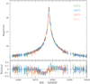 |
Fig. 1 Light curve of the lensing event KMT-2021-BLG-1077. The curve plotted over the data points is a single-lens single-source (1L1S) model obtained with the exclusion of the data lying in the anomaly region. The bottom panel shows the residual from the 1L1S model. The colors of the data points are set to match those of the data sets marked in the legend. |
3.1 Three-body models: 1L2S and 2L1S models
We first check whether or not the deviations from the 1L1S model can be explained by three-body (lens plus source) models, in which either the source or the lens is a binary. Hereafter, we denote lensing events associated with a binary source (Gaudi 1998; Dominik 1998; Han & Jeong 1998) and a binary lens (Mao & Paczyński 1991) as 1L2S and 2L1S events, respectively.
Modeling the lensing light curve of a 1L2S event requires the inclusion of three extra lensing parameters in addition to those of the 1L1S modeling, (t0,2, u0,2,qF), in which the first two represent the approach time and impact parameter of the second source, S2, to the lens, respectively, and the last parameter represents the flux ratio between the binary source stars. We denote the parameters related to the primary source, S1, as (t0,1, u0,1). In order to consider finite-source effects, which arise when the lens passes over the surface of either of the source stars, we additionally include the normalized source radii ρ1 and ρ2, which are defined as the ratios of the angular source radii, θ*,1 and θ*,2, to θΕ, that is, ρ1 = 0*,1 /θΕ and ρ2 = θ*,2./θE. The modeling was conducted by checking various trajectories of the second source with the consideration of the anomalous features in the 1L1S residual. For a given set of the initial lensing parameters related to S1, the best-fit 1L2S solution was searched for by minimizing; χ2 using a downhill approach based on the Markov chain Monte Carlo (MCMC) algorithm. The 1L2S modeling yields a model with lensing parameters of (t0,1, u0,1, t0,2, u0,2, tE, qF) ~ (9377.875,8.69 × 10−3,9378.807,8.98 × 10−3,25.6,0.104), and the normalized radii of both source stars are not constrained.
The residual from the best-fit 1L2S model is presented in Fig. 2. It shows that the model substantially reduces the residual from the 1L1S model by Δχ2 = 531.3, but the model still leaves noticeable residuals throughout the peak region. The residuals are characterized by negative deviations at a 0.05 mag level before t1, positive deviations of a similar level after t3, and a wiggly pattern with alternating positive and negative deviations in the region around t2. This indicates that the 1L2S model is not a correct interpretation of the anomaly.
Similar to the 1L2S case, a 2L1S modeling also requires three additional parameters to describe the lens binarity. These are (s, q, α), which denote the projected separation (scaled to (s, q, α) and mass ratio between the binary lens components, M1 and M2, and the source trajectory angle, which is defined as the angle between the direction of the source-lens relative motion and the binary axis, respectively. For this event, it is also necessary to include the normalized source size ρ = θ*,/θE in order to take into consideration finite-source effects. In the 2L1S modeling, we find a lensing solution in two steps, in which the binary parameters s and q were searched for via a grid approach and the other parameters were found via a downhill approach in the first step, and then local solutions found from the first step were polished by releasing all parameters as free parameters in the second step. It is found that the 2L1S interpretation does not yield a model describing all the features of the anomaly either.
We then checked whether or not a 2L1S model could partially explain the anomaly. We test this possibility because the central anomaly can be affected by an additional lens companion, if it exists, and in this case, a 2L1S model can often describe a part of the anomaly. For this test, we conducted two sets of 2L1S modeling in which the light curve was fitted by excluding the data lying in the regions of 9376.0 < HID′ < 9377.2 and 9378.2 < HID′ < 9379.4 in the first modeling, and by excluding those lying in the regions of 9377.0 < HID′ < 9378.0 and 9379.3 < HID′ < 9381.0 in the second modeling. We designate the solutions found from the modeling of the individual data sets as “solution 1” and “solution 2”, respectively. In Fig. 3, we present the model curves and residuals of solutions 1 and 2. The model and residuals of solution 1 showing all data are separately presented in Fig. 2. Figure 3 shows that solution 1 nicely explains the anomaly feature around the peak centered at t1, while solution 2 describes the bump around t3. The lensing parameters of the models are (s, q, α, ρ) ~ (1.31(1/1.31), 1.6 × 10−3,3.06, 5.4 × 10⁻³) for solution 1, and ~(0.98, 1.2 × 10⁻³, 2.46, 4.2 × 10⁻³) for solution 2. Here, the source trajectory angle is expressed in radians. For solution 1, we note that there exist two locals with binary separations of s ~ 1.31 and s ~ 1/1.31, for which the similarity in the lensing light curves between the two local solutions is caused by the well-known close–wide degeneracy arising due to the similarity between the central lensing caustics formed by binary lenses with s and 1/s (Griest & Safizadeh 1998; Dominik 1999; An 2005). Here, the caustics represent the source positions at which the lensing magnification of a point source becomes infinite. The two insets presented in the top panel of Fig. 3 show the lens system configurations of the individual solutions.
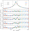 |
Fig. 2 Zoom-in view around the peak of the light curve. The lower five panels show the residuals of the tested models under 3L1S, 2L2S, 2L1S, 1L2S, and 1L1S interpretations. The curve drawn in each residual panel is the difference from the 3L1S model. The curves of the 1L1S, 2L1S, and 3L1S models are drawn over the data points of the light curve in the top panel. The epochs marked t1; t2, and t3 indicate the times of the major anomalous features. |
3.2 Four-body models: 2L2S and 3L1S models
Recognizing the inadequacy of the three-body models, we then examine two four-body models. In one of these, both the source and lens are binaries (2L2S model), and in the other, the lens is a triple system (3L1S model). In the 2L2S modeling, we add three binary-source parameters (t0,2, u0,2, qF) to those of the 2L1S model. In the 3L1S modeling, we add three tertiary-lens parameters (s3, q3, ψ), where s3 and q3 represent the separation and mass ratio between the third lens component, M3, and the primary, and ψ denotes the orientation angle of M3 as measured from the M1−M2 axis with a center at the position of M1. We add the subscript “2” to the lensing parameters describing M2, that is, (s2, q2), to distinguish them from those describing M3.
The 2L2S modeling was carried out by checking various trajectories of the second source under the basic lens-system configurations of the 2L1S models, that is, solutions 1 and 2 of the 2L1S models. In Fig. 2, we present the residual of the bestfit 2L2S model found based on solution 1 of the 2L1S model. The binary-source parameters of the solution are (t0,2, u0,2, qF) ~ (9378.811, 5.74 × 10⁻³, 0.042), and the other parameters are very similar to those of the 2L1S model. From inspection of the residual, we find that the model substantially reduces the 2L1S residuals in the region between t1 and t3 and improves the fit by Δχ2 = 327.1 with respect to the 2L1S model. However, the model still leaves subtle wiggles in the residual throughout the peak region. It is found that the 2L2S model obtained based on solution 2 of the 2L1S model results in a poorer fit than the model found based on solution 1.
We further checked the 3L1S interpretation of the anomaly. Similar to the 2L1S modeling, the 3L1S modeling was carried out in two steps. In the first round, we inspected the space of the tertiary lens parameters, that is, (s3, q3, ψ), via a grid approach by fixing the other lensing parameters as the values found from the 2L1S modeling. In the second round, we refined the locals found in the s3–q3–ψ planes by releasing all parameters as free parameters. This approach is based on the fact that the anomalies induced by two companions to the lens can, in many cases, be approximated by the superposition of the anomalies induced by the M1−M2 and M1−M3 binary pairs (Bozza 1999; Han et al. 2001).
Figure 4 shows the Δχ2 distribution on the log s3–log q3 parameter plane obtained from the grid searches for these parameters in the first round of the 3L1S modeling conducted based on solution 1 of the 2L1S model. It shows a single distinct local at (log s3, log q3) ~ (−0.01, −3, 0). The full lensing parameters of the 3L1S models after refining the local through the second round of the modeling are listed in Table 1. We note that α, that is, the angle between the source trajectory and the M1−M2 axis, is similar for the 3L1S model and for the 2L1S solution 1, while (α + ψ − 2π), that is, the angle between the source trajectory and the M1−M3 axis (additionally inserted in Table 1), for the 3L1S model is similar to the α for the 2L1S solution 2. We find two sets of 3L1S solutions, which are obtained from the modeling based on the close and wide 2L1S models of solution 1. We refer to the individual solutions as close and wide 3L1S solutions, between which the wide solution is favored over the close solution by Δχ2 = 43.4. It is found that the 3L1S model found on the basis of solution 2 of the 2L1S model is consistent with the 3L1S model obtained based on solution 1, except that the order of M2 and M3 is reversed.
It is found that the triple-lens interpretation yields a model that can explain all the major anomalous features in the lensing light curve. This can be seen in the model curve and the residual from the model presented in Figs. 2 and 3. We find that the wide 3L1S model yields a fit that is better than the 1L1S, 1L2S, 2L1S, and 2L2S models by Δχ2 = 937.0, 405.7, 486.4, and 159.3, respectively. In the residual panels of the other models in Fig. 2, we present the curves of the differences from the 3L1S model. The estimated mass ratios of the lens companions to the primary are q2 = M2/M1 ~ 1.56 × 10⁻³ and q3 = M3/M1 ~ 1.75 × 10⁻³. These mass ratios correspond to ~1.6 and ~1.8 times the Jupiter/Sun mass ratio, respectively, and therefore the lens is a multiplanetary system containing two giant planets.
Figure 5 displays the lens system configuration, which shows the source trajectory (line with an arrow) relative to the positions of the lens components (blue dots marked by M1, M2, and M3) and caustics (red cuspy figure). Although the close solution is disfavored with a significant χ2 difference from the wide solution, we present its lens system configuration for comparison with that of the wide solution. For each solution, the main panel shows a zoomed-in view of the central magnification region, and the inset shows the wider view encompassing all the lens components. The central caustic appears to be the combination of a tiny wedge-shaped central caustic induced by M2 and a bigger resonant caustic induced by M3. The similarities of the individual caustics to those of the 2L1S caustics of solutions 1 and 2, shown in the insets of the top panel of Fig. 3, indicate that the anomaly can be approximated by the superposition of the anomalies induced by the two planetary companions. According to the 3L1S interpretation, the negative deviation from the 1L1S model before t1 was produced by the source passage through the negative-deviation region extending from the back end of the M2-induced caustic. The source entered the resonant caustic induced by M3 at around t1, and passed along one of the caustic folds before it crossed the tip of the M1-induced caustic at around t2, which corresponds to the 1L1S residual bump at the corresponding time. The source further proceeded and exited the resonant caustic at t3, and this produced the second bump in the 1L1S residual at the corresponding time. We mark the source positions corresponding to the epochs of the major anomalous features at t1, t2, and t3 with empty magenta circles, whose size is proportionate to the source size.
According to the 3L1S solution, the passage of the source was almost parallel with the M1−M2 axis, with a source trajectory angle of α ~ 4.6°. This indicates the possibility that the source additionally approached the peripheral (planetary) caustic induced by M2, and we find that the source passed the region around the planetary caustic according to either the close or the wide model, roughly 15 days before or after the peak, respectively. See the insets of the panels presented in Fig. 5. If an additional anomaly were produced by this approach and captured by the data, it would further constrain the 3L1S interpretation. We therefore checked the data around the time of the anomaly expected by the individual models. Figure 6 shows the light curve around the regions of the anomalies predicted by the close (upper left panel) and wide (upper right panel) solutions. The light curve would exhibit a short-term dip and a bump at around HJD′ ~ 9362.5 and ~9391.5 according to the close and wide solutions, respectively. However, we find that it was difficult to confirm the additional anomaly in the light curve due to the large photometric uncertainties of the data around the regions, which lie close to the baseline. We note that the difficulty in identifying an extra anomaly may be caused by the orbital motion of the first planet, that is, M2. According to the Bayesian analysis of the physical lens parameters, which we discuss in Sect. 5, the host mass is about 0.14 M⊙, and the projected separation of the planet is about 0.8 AU and 1.4 AU according to the close and wide solutions, respectively. Hence in 15 days, it is expected for the orbital angle to change by ~6° and 2°.5 according to the individual solutions. Consequently, even if the static model predicted an extra anomaly, it might not appear in the light curve because the planet had moved due to its orbital motion.
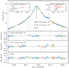 |
Fig. 3 Models and residuals of the “solution 1” and “solution 2” 2L1S models. The individual solutions are obtained from the two sets of 2L1S models, in which the light curve was fitted by excluding the data lying in the regions of 9376.0 < HID′ < 9377.2 and 9378.2 < HID′ < 9379.4 for solution 1, and by excluding those lying in the regions of 9377.0 < HID′ < 9378.0 and 9379.3 < HID′ < 9381.0 for solution 2. The two insets in the top panel show the lens system configurations of the individual solutions. Also presented are the model curve and residual of the 3L1S solution. |
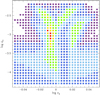 |
Fig. 4 Distribution of Δχ2 on the log s3–log q3 parameter plane. The color coding is arranged to denote regions with ≤ 1nσ (red), ≤ 2nσ (yellow), ≤ 3nσ (green), ≤ 4nσ (cyan), ≤ 5nσ (blue), and ≤ 6nσ (purple), where n = 3. |
Lensing parameters of the 3L1S models.
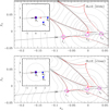 |
Fig. 5 Configuration of the lens system according to the wide (upper panel) and close (lower panel) 3L1S models. In each panel, the cuspy figure is the caustic and the line with an arrow indicates the source trajectory. The three empty magenta circles on the source trajectory represent the source positions corresponding to the three epochs of t1, t2, and t3 marked in Fig. 1. The size of the circle is proportionate to the source size. Lengths are normalized to the Einstein radius corresponding to the total lens mass. The inset in each panel shows a zoomed-out view, in which the locations of the individual lens components (M1, M2, and M3) and the Einstein ring (dotted circle) are marked. The curves encompassing the caustic represent the equi-magnification contours. |
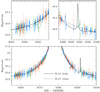 |
Fig. 6 Enlarged view of the light curve around the regions of the planetary-caustic induced anomalies predicted by the close (upper left panel) and wide (upper right panel) models. The bottom panel shows a zoomed-out view of the light curve at low magnification. The solid and dashed curves drawn over the data points are the wide and close 3L1S models, respectively. |
4 Source star and angular Einstein radius
For the lensing event KMT-2021-BLG-1077, it is possible to measure the extra observable of the angular Einstein radius because the anomaly in the lensing light curve was affected by finite-source effects. With the normalized source radius measured from the analysis of the anomaly, the Einstein radius is estimated as
 (1)
(1)
where θ*, is the angular radius of the source star. With the measured θE, together with the basic observable of the event timescale, the physical parameters of the lens mass, M, distance to the lens, DL, and lens-source relative proper motion μ can be constrained using the relations
 (2)
(2)
where κ = 4G/(c2AU) and DS indicates the distance to the source. If an additional lensing observable of the microlensparallax πE = (πrel/θE)(μ/μ) can be measured, the lens mass and distance are uniquely determined by
 (3)
(3)
where πS = AU/DS is the parallax of the source (Gould 1992, 2000). The microlens parallax can sometimes be measured from the subtle deviations in the lensing light curve caused by the positional change of an observer induced by the orbital motion of Earth around the Sun (Gould 1992). We find that it is difficult to securely constrain πE because the photometric precision of the data in the wings of the light curve is not sufficiently high to detect subtle deviations induced by the microlens-parallax effect.
For the measurement of θΕ, we first estimate the angular source radius, which is deduced from the color and magnitude of the source. Figure 7 shows the location of the source (blue solid dot) in the instrumental color-magnitude diagram (CMD) of stars lying in the vicinity of the source constructed from the pyDIA photometry (Albrow 2017) of the KMTC data. Also marked is the location of the blend (green dot). As discussed in Sect. 5, the blend is not the lens but a star (or stars) not involved with the lensing magnification. The I- and V-band source magnitudes were determined from the regression of the pyDIA data with the variation of the lensing magnification. Following the Yoo et al. (2004) method, we calibrate the source color and magnitude using the centroid of the red giant clump (RGC) marked by a red dot in Fig. 7 as a reference. From the offsets in color and magnitude between the source and RGC centroid, Δ(V − I, I), together with the known reddening and extinction-corrected (de-reddened) values of the RGC centroid, (V − I, I)rgc,0 = (1.060, 14.607) (Bensby et al. 2013; Nataf et al. 2013), we estimate the de-reddened source color and magnitude as
 (4)
(4)
indicating that the source is a late G-type main sequence star.
Once (V − I, I)0 are measured, we convert V − I color into V − K color using the color-color relation of Bessell & Brett (1988), and then interpolate θ* from the Kervella et al. (2004) relation between V − K and θ*. The angular radius of the source estimated from this procedure is
 (5)
(5)
The Einstein radius is then estimated from the relation in Eq. (1) as
 (6)
(6)
and the relative lens-source proper motion is estimated using the measured event time scale as
 (7)
(7)
We note that the values of θE and μ are estimated using the lensing parameters of the wide 3l1s solution because it is favored over the close solution with a significant level, that is, Δχ2 = 43.4. The estimated Einstein radius is substantially smaller than ~0.5 mas of a typical lensing event produced by a low-mass star with a mass of ~0.3 M⊙ lying roughly halfway between the source and observer. This suggests that the lens would either have a very low mass or lie close to the source.
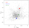 |
Fig. 7 Locations of the source (blue dot) and centroid of the red giant clump (red dot) on the instrumental color–magnitude diagram of stars lying around the source, constructed from the pyDIA photometry of the KMTC data set. Also marked is the location of the blend (green dot). |
5 Physical parameters of the planetary system
In this section, we estimate the physical parameters of the planetary system using the constraints provided by the measured observables of tE and θE. Not being able to uniquely constrain M and DL using the relations in Eq. (3) due to the absence of a πE constraint, we statistically estimate the parameters by conducting a Bayesian analysis using a Galactic model. The analysis is done based on the observables of the wide 3L1S solution.
The Galactic model defines the physical and dynamical distributions of stars and remnants in the Galaxy and their mass function (MF). We use the Galactic model of Jung et al. (2021), in which Robin et al. (2003) and Han & Gould (2003) models are used for the physical distributions of the disk and bulge objects, respectively; Jung et al. (2021) and Han & Gould (1995) models are adopted for the dynamical distributions of the disk and bulge objects, respectively; and the Jung et al. (2018) MF is employed for the MF of both disk and bulge objects. The MF model was constructed by adopting the initial MF and the present-day MF of Chabrier (2003) for the bulge and disk lens populations, respectively.
In the first step of the Bayesian analysis, we generate a large number (107) of artificial lensing events by conducting a Monte Carlo simulation using the Galactic model. For the individual simulated events, we then compute the values of the observables tE and θE using the relations in Eq. (2). In the second step, we construct the probability distributions of events by imposing Gaussian weight based on the measured values of the observables, that is, tE = (24.85 ± 0.73) days and θΕ = (0.13 ± 0.01) mas.
Figure 8 shows the Bayesian posteriors of the host mass, Mh, and the distances to the planetary system and the source star. In each distribution, we mark the median and uncertainty range of the distribution by a solid vertical line and dotted lines, respectively. The uncertainty range is estimated as the 16% and 84% of the distribution. The curves marked in blue and red indicate the disk and bulge lens contributions, respectively, and the black curve represents the sum of the contributions from the two lens populations. It is found that the relative probabilities of the disk and bulge lenses are 17% and 83%, respectively. We present the distribution of DS to show the relative positions of the lens and source. The distributions of DL and DS indicate that the event is likely to be produced by a star lying in the bulge, and the closeness between the lens and source explains the reason for the small Einstein radius. See the relation between θΕ and (Ds, Dl) in Eq. (2).
It is found that KMT-2021-BLG-1077L is a planetary system, in which a mid-to-late M dwarf star hosts two gas giant planets with masses of slightly less than that of Saturn in our Solar System. The estimated mass of the planet host is
 (8)
(8)
and the masses of the two planets are
 (9)
(9)
The planetary system is likely to be in the bulge with a distance from Earth of
 (10)
(10)
The projected separations of the individual planets from the host are
 (11)
(11)
Considering that the snow line distance is dsl = 2.7(Mh/M⊙) ~ 0.38 AU and the separations are projected ones, both planets lie well beyond the snow line of the host. If we assume that a = a⊥, then at face value, the system is not stable. However, a⊥ is simply the minimum possible value for the semi-major axis, and a stable system can easily be achieved simply by moving one or the other planet in or out of the plane of the sky. Madsen & Zhu (2019) explored the issue of stability for the OGLE-2012-BLG-0026L system. The ideas discussed in that paper are broadly applicable to systems such as KMT-2021-BLG-1077L, which appear at first glance to be unstable based on their projected separations.
The estimated host mass and distance indicate that the contribution of the lens flux to the blend, marked on the CMD in Fig. 7 (green solid dot), is negligible. This is additionally confirmed by the astrometric measurement of the offset between the source, measured on the difference image obtained during the lensing magnification, and the baseline object in the reference image. The offset, ~0.352 arcsec, is far larger than the measurement error, which is of the order of 10 mas.
The lens of the event KMT-2021-BLG-1077 is the fifth confirmed multiplanetary system detected by microlensing following OGLE-2006-BLG-109L, OGLE-2012-BLG-0026L, OGLE-2018-BLG-1011L, and OGLE-2019-BLG-0468L. It is the third multiplanetary system detected after the full operation of the high-cadence surveys. If the lenses of the events KMT-2019-BLG-1953 and KMT-2021-BLG-0240 – which exhibit relatively less-secure multi-planet signatures – are multiplanetary systems, the total number of multiplanetary systems detected by the six-year operation of the high-cadence surveys is five Considering that about 20 planets are annually detected by the surveys, this roughly matches the prediction of Zhu et al. (2014) that ~5.5% of planetary events that are detectable by the high-cadence surveys will exhibit multi-planet signals, although the number is too small to draw strong conclusions.
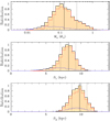 |
Fig. 8 Bayesian posteriors of the host mass (Mh), distances to the planetary system (DL), and source (DS). In each panel, the blue and red curves represent the contributions by the disk and bulge lenses, respectively, and the black curve is the sum of the two lens populations. The solid vertical line represents the median of the distribution, and the two dotted lines represent the 1σ range. |
6 Summary and conclusion
We present an analysis of the high-magnification microlensing event KMT-2021-BLG-1077, for which the peak region of the lensing light curve exhibited a subtle and complex anomaly pattern. The anomaly could not be explained by the usual three-body models, in which either the lens or the source is a binary. However, the anomaly can be explained by a lensing model in which the lens is composed of three masses.
With the constraints of the event timescale and angular Einstein radius, it is found that the lens is a multiplanetary system residing in the Galactic bulge. The primary of the lens system is a mid-to-late M dwarf and hosts two gas giant planets lying beyond the snow line of the host. The lens of the event is the fifth confirmed multiplanetary system detected using microlensing following OGLE-2006-BLG-109L, OGLE-2012-BLG-0026L, OGLE-2018-BLG-1011L, and OGLE-2019-BLG-0468L.
Acknowledgements
Work by C.H. was supported by the grants of National Research Foundation of Korea (2020R1A4A2002885 and 2019R1A2C2085965). This research has made use of the KMTNet system operated by the Korea Astronomy and Space Science Institute (KASI) and the data were obtained at three host sites of CTIO in Chile, SAAO in South Africa, and SSO in Australia. he MOA project is supported by JSPS KAKENHI grant Nos. JSPS24253004, JSPS26247023, JSPS23340064, JSPS15H00781, JP16H06287, JP17H02871, and JP19KK0082. J.C.Y. acknowledges support from NSF Grant No. AST-2108414. C.R. was supported by the Research fellowship of the Alexander von Humboldt Foundation.
References
- Alard, C., & Lupton, R.H. 1998, ApJ, 503, 325 [NASA ADS] [CrossRef] [Google Scholar]
- Albrow, M. 2017, https://doi.org/10.5281/zenodo.268049 [Google Scholar]
- Albrow, M., Horne, K., Bramich, D.M., et al. 2009, MNRAS, 397, 2099 [NASA ADS] [CrossRef] [Google Scholar]
- An, J.H. 2005, MNRAS, 356, 1409 [NASA ADS] [CrossRef] [Google Scholar]
- Beaulieu, J.-P., Bennett, D.P., Batista, V., et al. 2016, ApJ, 824, 83 [CrossRef] [Google Scholar]
- Beaulieu, J.-P., Bennett, D.P., Fouqué, P., et al. 2006, Nature, 439, 437 [NASA ADS] [CrossRef] [Google Scholar]
- Bennett, D.P., Rhie, S.H., Nikolaev, S., et al. 2010, ApJ, 713, 837 [NASA ADS] [CrossRef] [Google Scholar]
- Bensby, T., Yee, J.C., Feltzing, S., et al. 2013, A&A, 549, A147 [NASA ADS] [CrossRef] [EDP Sciences] [Google Scholar]
- Bessell, M.S., & Brett, J.M. 1988, PASP, 100, 1134 [NASA ADS] [CrossRef] [Google Scholar]
- Blackman, J.W., Beaulieu, J.P., Bennett, D.P., et al. 2021, Nature, 598, 272 [NASA ADS] [CrossRef] [Google Scholar]
- Bond, I.A., Abe, F., Dodd, R.J., et al. 2001, MNRAS, 327, 868 [NASA ADS] [CrossRef] [Google Scholar]
- Bozza, V. 1999, A&A, 348, 311 [NASA ADS] [Google Scholar]
- Chabrier, G. 2003, PASP, 115, 763 [Google Scholar]
- Dominik, M. 1998, A&A, 333, 893 [NASA ADS] [Google Scholar]
- Dominik, M. 1999, A&A, 349, 108 [NASA ADS] [Google Scholar]
- Gaudi, B.S. 1998, ApJ, 506, 533 [NASA ADS] [CrossRef] [Google Scholar]
- Gaudi, B.S. 2012, ARA&A, 50, 411 [NASA ADS] [CrossRef] [Google Scholar]
- Gaudi, B.S., Naber, R.M., & Sackett, P.D. 1998, ApJ, 502, L33 [CrossRef] [Google Scholar]
- Gaudi, B.S., Bennett, D.P., Udalski, A., et al. 2008, Science, 319, 927 [NASA ADS] [CrossRef] [Google Scholar]
- Gould, A. 1992, ApJ, 392, 442 [Google Scholar]
- Gould, A. 2000, ApJ, 542, 785 [NASA ADS] [CrossRef] [Google Scholar]
- Gould, A., Udalski, A., An, D., et al. 2006, ApJ, 644, L37 [Google Scholar]
- Griest, K., & Safizadeh, N. 1998, ApJ, 500, 37 [Google Scholar]
- Han, C. 2005, ApJ, 629, 1102 [NASA ADS] [CrossRef] [Google Scholar]
- Han, C., & Gould, A. 1995, ApJ, 447, 53 [Google Scholar]
- Han, C., & Gould, A. 2003, ApJ, 592, 172 [Google Scholar]
- Han, C., & Jeong, Y. 1998, MNRAS, 301, 231 [NASA ADS] [CrossRef] [Google Scholar]
- Han, C., Chang, H.-Y., An, J.H., & Chang, K. 2001, MNRAS, 328, 986 [NASA ADS] [CrossRef] [Google Scholar]
- Han, C., Udalski, A., Choi, J.-Y., et al. 2013, ApJ, 762, L28 [Google Scholar]
- Han, C., Bennett, D.P., Udalski, A., et al. 2019, AJ, 158, 114 [NASA ADS] [CrossRef] [Google Scholar]
- Han, C., Kim, D., Jung, Y.K., et al. 2020, AJ, 160, 17 [NASA ADS] [CrossRef] [Google Scholar]
- Han, C., Kim, D., Yang, H., et al. 2022a, A&A, accepted, https://doi.org/10.1051/0004-6361/202243161 [Google Scholar]
- Han, C., Udalski, A., Lee, C.-U., et al. 2022b, A&A, 658, A93 [NASA ADS] [CrossRef] [EDP Sciences] [Google Scholar]
- Ida, S., & Lin, D.N.C. 2010, ApJ, 719, 810 [NASA ADS] [CrossRef] [Google Scholar]
- Jung, Y.K., Udalski, A., Gould, A., et al. 2018, AJ, 155, 219 [NASA ADS] [CrossRef] [Google Scholar]
- Jung, Y.K., Han, C., Udalski, A., et al. 2021, AJ, 161, 293 [NASA ADS] [CrossRef] [Google Scholar]
- Kervella, P., Thévenin, F., Di Folco, E., & Ségransan, D. 2004, A&A, 426, 29 [Google Scholar]
- Kim, S.-L., Lee, C.-U., Park, B.-G., et al. 2016, JKAS, 49, 37 [Google Scholar]
- Kim, D.-J., Hwang, K.-H., Shvartzvald, et al. 2018, AAS, submitted [arXiv:1806.07545] [Google Scholar]
- Madsen, S., & Zhu, W. 2019, ApJ, 878, L29 [NASA ADS] [CrossRef] [Google Scholar]
- Mao, S., & Paczynski, B. 1991, ApJ, 374, L37 [NASA ADS] [CrossRef] [Google Scholar]
- Mróz, Przemek, Ryu, Y.-H., Skowron, J., et al. 2018, AJ, 155, 121 [CrossRef] [Google Scholar]
- Nataf, D.M., Gould, A., Fouqué, P., et al. 2013, ApJ, 769, 88 [NASA ADS] [CrossRef] [Google Scholar]
- Robin, A.C., Reylé, C., Derriére, S., & Picaud, S. 2003, A&A, 409, 523 [NASA ADS] [CrossRef] [EDP Sciences] [Google Scholar]
- Ryu, Y.-H., Mröz, P., Gould, A., et al. 2021, AJ, 161, 126 [NASA ADS] [CrossRef] [Google Scholar]
- Shvartzvald, Y., Yee, J.C., Calchi Novati, S., et al. 2017, ApJ, 840, L3 [NASA ADS] [CrossRef] [Google Scholar]
- Szymanski, M.K., Udalski, A., Soszynski, I., et al. 2011, Acta Astron., 61, 83 [NASA ADS] [Google Scholar]
- Suzuki, D., Bennett, D.P., Udalski, A., et al. 2018, AJ, 155, 263 [NASA ADS] [CrossRef] [Google Scholar]
- Tomaney, A.B., & Crotts, A.P.S. 1996, AJ, 112, 2872 [NASA ADS] [CrossRef] [Google Scholar]
- Yee, J.C., Shvartzvald, Y., Gal-Yam, A., et al. 2012, ApJ, 755, 102 [NASA ADS] [CrossRef] [Google Scholar]
- Yoo, J., DePoy, D.L., Gal-Yam, A., et al. 2004, ApJ, 603, 139 [NASA ADS] [CrossRef] [Google Scholar]
- Zang, W., Han, C., Kondo, I., et al. 2021, Res. Astron. Astrophys., 21, 239 [CrossRef] [Google Scholar]
- Zhu, W., Penny, M., Mao, S., Gould, A., & Gendron, R. 2014, ApJ, 788, 73 [Google Scholar]
All Tables
All Figures
|
Fig. 1 Light curve of the lensing event KMT-2021-BLG-1077. The curve plotted over the data points is a single-lens single-source (1L1S) model obtained with the exclusion of the data lying in the anomaly region. The bottom panel shows the residual from the 1L1S model. The colors of the data points are set to match those of the data sets marked in the legend. |
| In the text | |
|
Fig. 2 Zoom-in view around the peak of the light curve. The lower five panels show the residuals of the tested models under 3L1S, 2L2S, 2L1S, 1L2S, and 1L1S interpretations. The curve drawn in each residual panel is the difference from the 3L1S model. The curves of the 1L1S, 2L1S, and 3L1S models are drawn over the data points of the light curve in the top panel. The epochs marked t1; t2, and t3 indicate the times of the major anomalous features. |
| In the text | |
|
Fig. 3 Models and residuals of the “solution 1” and “solution 2” 2L1S models. The individual solutions are obtained from the two sets of 2L1S models, in which the light curve was fitted by excluding the data lying in the regions of 9376.0 < HID′ < 9377.2 and 9378.2 < HID′ < 9379.4 for solution 1, and by excluding those lying in the regions of 9377.0 < HID′ < 9378.0 and 9379.3 < HID′ < 9381.0 for solution 2. The two insets in the top panel show the lens system configurations of the individual solutions. Also presented are the model curve and residual of the 3L1S solution. |
| In the text | |
|
Fig. 4 Distribution of Δχ2 on the log s3–log q3 parameter plane. The color coding is arranged to denote regions with ≤ 1nσ (red), ≤ 2nσ (yellow), ≤ 3nσ (green), ≤ 4nσ (cyan), ≤ 5nσ (blue), and ≤ 6nσ (purple), where n = 3. |
| In the text | |
|
Fig. 5 Configuration of the lens system according to the wide (upper panel) and close (lower panel) 3L1S models. In each panel, the cuspy figure is the caustic and the line with an arrow indicates the source trajectory. The three empty magenta circles on the source trajectory represent the source positions corresponding to the three epochs of t1, t2, and t3 marked in Fig. 1. The size of the circle is proportionate to the source size. Lengths are normalized to the Einstein radius corresponding to the total lens mass. The inset in each panel shows a zoomed-out view, in which the locations of the individual lens components (M1, M2, and M3) and the Einstein ring (dotted circle) are marked. The curves encompassing the caustic represent the equi-magnification contours. |
| In the text | |
|
Fig. 6 Enlarged view of the light curve around the regions of the planetary-caustic induced anomalies predicted by the close (upper left panel) and wide (upper right panel) models. The bottom panel shows a zoomed-out view of the light curve at low magnification. The solid and dashed curves drawn over the data points are the wide and close 3L1S models, respectively. |
| In the text | |
|
Fig. 7 Locations of the source (blue dot) and centroid of the red giant clump (red dot) on the instrumental color–magnitude diagram of stars lying around the source, constructed from the pyDIA photometry of the KMTC data set. Also marked is the location of the blend (green dot). |
| In the text | |
|
Fig. 8 Bayesian posteriors of the host mass (Mh), distances to the planetary system (DL), and source (DS). In each panel, the blue and red curves represent the contributions by the disk and bulge lenses, respectively, and the black curve is the sum of the two lens populations. The solid vertical line represents the median of the distribution, and the two dotted lines represent the 1σ range. |
| In the text | |
Current usage metrics show cumulative count of Article Views (full-text article views including HTML views, PDF and ePub downloads, according to the available data) and Abstracts Views on Vision4Press platform.
Data correspond to usage on the plateform after 2015. The current usage metrics is available 48-96 hours after online publication and is updated daily on week days.
Initial download of the metrics may take a while.