| Issue |
A&A
Volume 670, February 2023
|
|
|---|---|---|
| Article Number | A172 | |
| Number of page(s) | 9 | |
| Section | Galactic structure, stellar clusters and populations | |
| DOI | https://doi.org/10.1051/0004-6361/202245525 | |
| Published online | 22 February 2023 | |
OGLE-2018-BLG-0584 and KMT-2018-BLG-2119: Two microlensing events with two lens masses and two source stars
1
Department of Physics, Chungbuk National University, Cheongju 28644, Republic of Korea
e-mail: cheongho@astroph.chungbuk.ac.kr
2
Astronomical Observatory, University of Warsaw, Al. Ujazdowskie 4, 00-478 Warszawa, Poland
3
Korea Astronomy and Space Science Institute, Daejon 34055, Republic of Korea
4
Department of Astronomy and Tsinghua Centre for Astrophysics, Tsinghua University, Beijing 100084, PR China
5
University of Canterbury, Department of Physics and Astronomy, Private Bag 4800, Christchurch 8020, New Zealand
6
Korea University of Science and Technology, 217 Gajeong-ro, Yuseong-gu, Daejeon 34113, Republic of Korea
7
Max Planck Institute for Astronomy, Königstuhl 17, 69117 Heidelberg, Germany
8
Department of Astronomy, The Ohio State University, 140 W. 18th Ave., Columbus, OH 43210, USA
9
Department of Particle Physics and Astrophysics, Weizmann Institute of Science, Rehovot 76100, Israel
10
Center for Astrophysics, Harvard & Smithsonian 60 Garden St., Cambridge, MA 02138, USA
11
School of Space Research, Kyung Hee University, Yongin, Kyeonggi 17104, Republic of Korea
12
Department of Astronomy & Space Science, Chungbuk National University, Cheongju 28644, Republic of Korea
13
Department of Physics & Astronomy, Seoul National University, Seoul 08826, Republic of Korea
14
Department of Physics, University of Warwick, Gibbet Hill Road, Coventry CV4 7AL, UK
Received:
21
November
2022
Accepted:
27
December
2022
Aims. We conducted a systematic investigation of the microlensing data collected during the previous observation seasons for the purpose of re-analyzing anomalous lensing events with no suggested plausible models.
Methods. We found that two anomalous lensing events, OGLE-2018-BLG-0584 and KMT-2018-BLG-2119, cannot be explained with the usual models based on either a binary-lens single-source (2L1S) or a single-lens binary-source (1L2S) interpretation. We tested the feasibility of explaining the light curves of the events with more sophisticated models by adding either an extra lens (3L1S model) or a source (2L2S model) component to the 2L1S lens system configuration.
Results. We find that a 2L2S interpretation explains the light curves of both events well and that for each event there are a pair of solutions resulting from the close and wide degeneracy. For the event OGLE-2018-BLG-0584, the source is a binary composed of two K-type stars and the lens is a binary composed of two M dwarfs. For KMT-2018-BLG-2119, the source is a binary composed of two dwarfs of G and K spectral types and the lens is a binary composed of a low-mass M dwarf and a brown dwarf.
Key words: binaries: general / gravitational lensing: micro
© The Authors 2023
 Open Access article, published by EDP Sciences, under the terms of the Creative Commons Attribution License (https://creativecommons.org/licenses/by/4.0), which permits unrestricted use, distribution, and reproduction in any medium, provided the original work is properly cited.
This article is published in open access under the Subscribe to Open model. Subscribe to A&A to support open access publication.
1. Introduction
Since the pioneering works of the first-generation experiments, for example, OGLE (Udalski et al. 1994), MACHO (Alcock et al. 1993), and EROS (Aubourg et al. 1993) surveys conducted in the early 1990s, searches for light variations of stars induced by gravitational lensing have been carried out for more than three decades by multiple groups succeeding earlier experiments. With the upgrade of instruments and observational strategy, the detection rate of lensing events has dramatically increased from a few dozen in the early surveys to several thousands in the current lensing surveys that are being carried out by the OGLE-IV (Udalski et al. 2015), MOA (Bond et al. 2001), and KMTNet (Kim et al. 2016) groups.
Light curves of most lensing events follow the smooth and symmetric form of a single-lens single-source (1L1S) event (Paczyński 1986). For a fraction of events, light curves exhibit deviations from the 1L1S form, and these deviations are, in most cases, caused by the binarity of the lens, 2L1S events (Mao & Paczyński 1991), or the binarity of the source, 1L2S events (Griest & Hu 1993; Han & Gould 1997).
With the increased number of lensing events, it is occasionally found that deviations in lensing light curves cannot be explained by the usual 2L1S or 1L2S forms. One important cause of such deviations is the existence of an extra lens component, that is, when the lens is composed of three masses (3L1S event), as first suggested by Gaudi et al. (1998) and theoretically investigated by Daněk & Heyrovský (2015a,b, 2019. Another major cause is that the source is a binary composed of two stars, and thus both the lens and source are binaries (2L2S event). At the time of writing this paper, there exist 18 lensing events with four or more bodies (lens+source), and among them 12 are 3L1S events, one is a 3L2S event, and the other 5 are 2L2S events. In Table 1, we list these lensing events and provide a brief summary of the anomaly types and related references.
Microlensing events with four or more bodies.
In this paper, we report on two lensing events that involve binary lens and binary source stars: OGLE-2018-BLG-0584 and KMT-2018-BLG-2119. In the current lensing surveys, anomalous lensing events are being analyzed by multiple modelers almost in real time with the progress of events, and microlensing models found from such analyses are circulated to the microlensing community or posted on web pages1. At this stage, events are mostly analyzed with the relatively simple 2L1S or 1L2S model, and thus events involving four or more bodies are, in most cases, left without any suggested models describing their observed anomalies. We found the 2L2S nature of OGLE-2018-BLG-0584 and KMT-2018-BLG-2119 from a systematic investigation of anomalous lensing events that have not had any plausible 2L1S or 1L2S models. Beyond these events, we also identified one event, KMT-2021-BLG-1122, that was produced by a triple-lens system. The analysis for this 3L1S event will be presented in a separate paper (Han et al. 2023).
We present the analyses of the two 2L2S events according to the following organization. In Sect. 2, we describe the observations conducted for the individual events and the data acquired from the observations. In Sect. 3, we explain various lensing models tested in the analyses and explain the detailed procedure of the light curve modeling. In the subsequent subsections, we present the analysis conducted for the individual events: OGLE-2018-BLG-0584 in Sect. 3.1 and KMT-2018-BLG-2119 in Sect. 3.2. In Sect. 4, we depict the procedures for defining the source stars and estimating the angular Einstein radii of the events. In Sect. 5, we describe the Bayesian analyses conducted using the observables of the individual lensing events and list the physical lens parameters estimated from the analyses. We summarize results from the analyses and conclude in Sect. 6.
2. Observations and data
The lensing events OGLE-2018-BLG-0584 and KMT-2018-BLG-2119 were found in the surveys of the Galactic bulge conducted in the 2018 season. Observations of the event OGLE-2018-BLG-0584 were done by the OGLE and KMTNet groups. The source of the event lies at (RA, Dec)J2000 = (17 : 53 : 36.29, −31 : 19 : 42.60), which corresponds to the Galactic coordinates of  . The first alert of the event was issued by the OGLE group on 2018 April 12 (HJD′≡HJD − 2450000 = 8219) when the source was brighter than the baseline magnitude, Ibase = 19.65, by ΔI ∼ 0.3 mag. The event occurred before the full operation of the KMTNet AlertFinder (Kim et al. 2018b) system, and it was found during the post-season inspection of the data using the KMTNet EventFinder system (Kim et al. 2018a). In the KMTNet alert web page2, the event is designated as KMT-2018-BLG-2006. Following the convention of the microlensing community of using a representative event ID reference of the first discovery group, we hereafter designate the event as OGLE-2018-BLG-0584. The event KMT-2018-BLG-2119, in contrast, was found solely by the KMTNet group from the post-season analysis of the 2018 season data. The equatorial and Galactic coordinates of the source are (RA, Dec)J2000 = (17 : 56 : 47.62, −28 : 40 : 59.99) and
  , respectively. The source is very faint, making it difficult to measure its baseline magnitude in the KMTNet template image, but it is registered in the OGLE-III Catalog with a magnitude of Icat = 21.38.
Observations of the events were conducted using the telescopes operated by the OGLE and KMTNet lensing surveys. The OGLE group employs a single 1.3 m telescope, and the KMTNet group utilizes three identical 1.6 m telescopes for surveys. The OGLE telescope is located at the Las Campanas Observatory in Chile, and the KMTNet telescopes are at three separate sites: One is at the Siding Spring Observatory in Australia (KMTA), another is at the Cerro Tololo Interamerican Observatory in Chile (KMTC), and the third is at the South African Astronomical Observatory in South Africa (KMTS). The cameras mounted on the OGLE and KMTNet telescopes have 1.4 deg2 and 4 deg2 fields of view, respectively.
Images of the source stars were mainly obtained in the I band, and a fraction of images were acquired in the V band for the source color measurements. Reductions of data and photometry of the source stars were carried out using the pipelines of the individual groups developed by Udalski (2003) for the OGLE survey and by Albrow et al. (2009) for the KMTNet survey. Additional photometry was done for the KMTC data set using the pyDIA code (Albrow 2017) to construct color-magnitude diagrams (CMDs) of stars lying around the source stars and to estimate the source magnitudes in the I and V passbands. (See more detailed discussion in Sect. 4.) Following the routine described in Yee et al. (2012), we readjusted the error bars of the photometry data estimated by the pipelines so that the error bars were consistent with the scatter of the data and the χ2 per degree of freedom (d.o.f.) for each data set became unity.
3. Analyses
The analyses of the events were carried out in two steps. In the first step, we modeled the light curves of the events with either a 2L1S or a 1L2S model. If neither of these models could explain the data, we then tested more sophisticated models that included an extra lens (3L1S model) or an extra source (2L2S model) component to the 2L1S lens system configuration.
In the modeling, we searched for a lensing solution that represents a set of lensing parameters depicting the configuration of the lens system. In the simplest case of a 1L1S event, the lensing light curve is described by three parameters (t0, u0, tE), which represent the time of the closest source approach to the lens, the projected lens–source separation at that time (impact parameter), and the Einstein timescale, respectively. The Einstein timescale is defined as the time required for a source to transit the angular Einstein radius θE of a lens. The length of the impact parameter was scaled to θE.
A 2L1S model requires four parameters (s, q, α, ρ) in addition to those of the 1L1S model. The first two parameters, s and q, indicate the projected separation (normalized to θE) and mass ratio between the lens components M1 and M2, respectively, and α represents the angle between the direction of the relative lens-source proper motion μ and the M1–M2 axis (source trajectory angle). The last parameter, ρ, which is defined as the ratio of the angular source radius θ* to θE, that is, ρ = θ*/θE (normalized source radius), describes the deformation of a lensing light curve by finite-source effects during the crossing of a source over the caustic formed by a binary lens system (Bennett & Rhie 1996).
A 1L2S model also requires extra parameters. These extra parameters are (t0, 2, u0, 2, qF). The first two represent the peak time and impact parameter of the source companion (S2) to the primary source (S1), and the last parameter denotes the flux ratio between S1 and S2 (Hwang et al. 2013). In the 1L2S modeling, we used the notations (t0, 1, u0, 1) to designate the parameters related to S1.
Adding a tertiary lens component (M3) to a 2L1S configuration requires three additional parameters (s3, q3, ψ) (Han et al. 2013). These parameters represent the projected separation and mass ratio between M1 and M3 and the position angle of the third body as measured from the M1–M2 axis centered at the position of M1, respectively. In order to distinguish the parameters related to M2 from those describing M3, we used the notations (s2, q2) to designate the separation and mass ratio between M1 and M2.
Similarly, adding a second source to a 2L1S configuration requires extra parameters in modeling. These parameters are (t0, 2, u0, 2, ρ2, qF). Here we used the subscript “2” to designate the parameters related to the second source and the subscript “1” to denote the parameters related to the primary source, that is, (t0, 1, u0, 1, ρ1). In Table 2, we summarize the lensing parameters of the models tested in our analyses together with the total numbers of parameters, Npar, included in the individual models.
Lensing parameters of tested models.
The three-body (2L1S and 1L2S) modeling was conducted considering the patterns of the anomalies appearing in the light curves. In the 2L1S modeling, we initially searched for the binary parameters (s, q) via a grid approach, while the other parameters were found via a downhill approach using a Markov chain Monte Carlo (MCMC) logic, constructing an χ2 map on the log s–log q plane, identifying local solutions on the χ2 map, and then refining the individual local solutions by allowing all parameters to vary. In the 1L2S modeling, we first fit the light curve with a 1L1S model, then obtained approximate values of the 1L1S parameters, and finally tested various configurations of the second source considering the time, magnitude, and pattern of the anomaly. As is discussed in the following subsections, we found that the light curves of the OGLE-2018-BLG-0584 and KMT-2018-BLG-2119 events cannot be precisely described by either of the three-body models.
Although the anomalies cannot be fully described by three-body models, we found that 2L1S models can partially describe the anomalies for both events. The light curve of a 2L2S event is the superposition of the light curves of the two 2L1S events involved with the individual source stars. Similarly, the anomalies induced by a triple-lens system, in many cases, are known to be approximated as the superposition of the anomalies induced by the two binary pairs, that is, M1–M2 and M1–M3 pairs (Bozza 1999; Han et al. 2021). The four-body modeling was conducted under this superposition approximation by first finding a 2L1S model of each event that described a part of the anomaly. Based on this 2L1S model, we conducted a 2L2S modeling by testing various trajectories of the second source, considering the anomaly part that could not be explained by the 2L1S model. For the 3L1S model, we first conducted grid searches for the perimeters related to M3, that is, (s3, q3, ψ), with the other parameters fixed as the values found from the 2L1S model, and we then refined the lensing solutions found from the grid search by letting all parameters vary. In the following subsections, we explain details of the modeling conducted for the two events and present the best solutions for explaining the anomalies of the individual events.
3.1. OGLE-2018-BLG-0584
The light curve of the lensing event OGLE-2018-BLG-0584 is shown in Fig. 1. It is characterized by two distinctive anomaly features centered at HJD′∼8224.3 (t1) and ∼8224.7 (t2). Based on the sharp rise and fall of the source flux and the non-smooth curvature in the light curve around the anomalies, it is likely that both anomalies were produced by caustic crossings of a source. The event lies in the two overlapping prime KMTNet fields of BLG01 and BLG41 toward which observations were conducted with a combined cadence of 0.25 h. Thus the rising part of the first anomaly feature and both the rising and falling parts of the second anomaly feature are densely covered by the data.
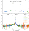 |
Fig. 1. Light curve of OGLE-2018-BLG-0584. The curve drawn over the data points is the model of the close 2L1S solution found from the fit of the data excluding those in the region 8224.5 ≤ HJD − 2450000 ≤ 8225.5. The upper panel shows the zoom of the anomaly region. |
Because caustics are produced by a multiple lens system, we excluded the 1L2S interpretation and started the analysis of the light curve with a 2L1S model. Despite a thorough investigation of the parameter space, we found no 2L1S solution that simultaneously described both anomalies. We then checked whether a 2L1S model could describe either of the anomalies. For this check, we conducted additional 2L1S modeling by fitting the light curve with the exclusion of the data around the second anomaly lying in the range of 8224.5 ≤ HJD′≤8225.5. From this, we found a pair of 2L1S models that could describe the first anomaly of the light curve. The two solutions with binary parameters of (s, q)close ∼ (0.6, 0.6) and (s, q)wide ∼ (2.4, 1.1) result from the close–wide degeneracy (Dominik 1999; An 2005). In Figs. 1 and 2, we have drawn the model curve over the data points for one (wide solution) of the two 2L1S solutions. The lens system configurations of the two 2L1S solutions are shown in the insets of the top panel in Fig. 2.
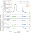 |
Fig. 2. Comparisons of models in anomaly region of OGLE-2018-BLG-0584 light curve. The top panel shows the four models of the close and wide 2L2S, 3L1S, and 2L1S solutions, and the lower panels show the residuals from the individual models. The three insets in the top panel show the lens system configurations of the 2L1S and 3L1S solutions. In each inset, the red figures represent the caustics and the line with an arrow indicates the source trajectory. The configuration of the 2L2S solutions are presented in Fig. 3. |
We further checked whether the data around the second anomaly could be explained with the introduction of a tertiary lens component. The model curve and residual of the best-fit 3L1S solution are presented in Fig. 2. We also present the lens system configuration of the 3L1S solution in the inset of the top panel. We found that the 3L1S model approximately describes both anomaly features at around t1 and t2, but it leaves systematic, subtle negative residuals in the region around the first anomaly and positive residuals in the region around the second anomaly, indicating that another interpretation is needed for the precise description of the anomalies.
We additionally tested a 2L2S interpretation of the anomalies by adding an extra source component to the 2L1S model. From this test, we found that both anomalies were well explained by a 2L2S interpretation. We identified two 2L2S solutions that resulted from the initial parameters of the close and wide 2L1S solutions. The lensing parameters of the individual solutions, which we refer to as “close” (s > 1.0) and “wide” (s > 1.0) solutions, are listed in Table 3 together with the values of χ2/d.o.f.. For the values of tE, ρ1, and ρ2 of the wide solution, we additionally present the values scaled to the Einstein radius of the lens component lying closer to the source trajectory, values in the parentheses, to show that these values are similar to those of the close solution. The fits of the two solutions are nearly the same, and the wide solution is preferred over the close solution by a mere Δχ2 = 2.3. Although the binary parameters (s, q) of the two degenerate solutions are substantially different from each other, the flux ratios between the source stars, qF ∼ 0.28, estimated by the two degenerate solutions are similar to each other.
2L2S models of OGLE-2018-BLG-0584.
The lens system configuration of the 2L2S model is shown in Fig. 3. The configuration is similar to those of the corresponding 2L1S models, shown in the top-panel insets of Fig. 2, except that there is an additional trajectory of the second source (“S2”) that trails the primary source (“S1”) with a small separation. According to the models, the anomaly at t2, which could not be explained by the 2L1S models, was produced by the crossing of S2 over the tip of the caustic with an impact parameter slightly greater than that of S1. We found that the 2L2S model yields a better fit than the 3L1S model by Δχ2 = 220.1, and this strongly supports the 2L2S interpretation of the anomaly.
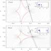 |
Fig. 3. Lens system configurations for the close (upper panel) and wide (lower panel) 2L2S solutions of OGLE-2018-BLG-0584. In each panel, the close figure represents the caustic, and the two lines with arrows marked by S1 and S2 represent the trajectories of the primary (S1) and secondary (S2) source stars. The grey curves encompassing the caustic represent the equimagnification contours. The inset in each panel shows the whole view of the lens system, where the blue dots represent the positions of the binary lens components and the dotted circle is the Einstein ring. |
According to the close 2L2S solution, the separation between the two source stars is Δu = {(u0, 1 − u0, 2)2 + [(t0, 1 − t0, 2)/tE]2}1/2 ∼ 0.044. As is discussed in Sect. 4, the angular Einstein radius is θE ∼ 0.57 mas. By adopting the distance to the source of DS ∼ 8 kpc, the two stars of the binary source were separated by a⊥ = ΔuDSθE ∼ 0.20 AU in projection, and probably a ∼ 0.25 AU in three-dimensional space. Assuming that the intrinsic separation is a = 0.25 AU, the orbital period of the source would be about  days where we adopt the total mass of the source of MS, tot ∼ 1.8 M⊙, considering the stellar types of the source stars discussed in Sect. 4. This orbital period is long enough to ignore source orbital motion because the anomaly lasted only about two days.
3.2. KMT-2018-BLG-2119
The light curve of the lensing event KMT-2018-BLG-2119 is presented in Fig. 4. It shows a strong anomaly appearing about two days after the peak, and the anomaly is characterized by three features: a weak bump at HJD′∼8378 (t1) and two strong features at ∼8380.4 (t2) and ∼8381.0 (t3). From the discontinuous derivatives of the source flux, the features around t2 and t3 are likely to be involved with a caustic, and these anomaly features exclude the 1L2S interpretation of the light curve. Despite the fact that the source of the event lies in the two overlapping KMTNet prime fields of BLG02 and BLG42, toward which the event was covered with a high combined cadence of 0.25 h, the features at around the peak of the anomaly were only partially covered. This was not only because the observing window at the time of the anomaly (around September 17) was short but also because the sky in South Africa was cloudy during the anomaly.
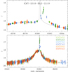 |
Fig. 4. Light curve of KMT-2018-BLG-2119. The curve drawn over the data points is a 2L1S model (close solution) obtained by fitting the light curve with the exclusion of the data in the region of 8380.7 ≤ HJD′≤8384.0. |
As in the case of OGLE-2018-BLG-0584, we found that a 2L1S model could not precisely describe all the anomaly features. In order to check whether a 2L1S model could provide a partial description of the anomaly, we divided the anomaly into two parts. The first part includes the features around t1 and t2, and the second part includes the feature around t3. We then fit the light curve by excluding the data around the second part lying in the range of 8380.7 ≤ HJD′≤8384.0. From this modeling, we found that the anomaly features in the first part were well explained by a pair of 2L1S models resulting from the close–wide degeneracy with (s, q)close ∼ (0.32, 0.13) and (s, q)wide ∼ (2.53, 0.11). The model curve of the close solution is drawn over the data points in Figs. 4 and 5, and the lens system configurations of the close and wide solutions are presented in the insets of the top panel in Fig. 5. According to these solutions, the first part of the anomaly is explained by the approach of the source close to the upper cusp of the caustic, producing the weak anomaly at around t1, and the subsequent passage of the source through the protruding right-side tip of the caustic, producing the sharp anomaly feature at around t2. The KMTC data around t2 correspond to the falling side of the caustic crossing.
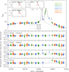 |
Fig. 5. Comparison of models in the anomaly region of the KMT-2018-BLG-2119 light curve. Notations are the same as those in Fig. 2. |
For the explanation of the whole anomaly features, we tested a 3L1S interpretation by modeling the light curve with the use of the initial lensing parameters from the 2L1S modeling. The model curve of the best-fit 3L1S solution and its residual are shown in Fig. 5 together with the lens-system configuration of the solution, shown in the inset of the top panel. We found that the model could not precisely describe the anomaly features, although it approximately delineated the feature at around t3.
We further tested a 2L2S interpretation of the anomaly by adding an extra source to the 2L1S system. From this, we found that all the features of the anomaly were well explained by this model. We found a pair of solutions obtained with the initial parameters of the close and wide 2L1S solutions. The full lensing parameters of the close and wide solutions are listed in Table 4, and the model curve of the close solution and residuals of both solutions are shown in Fig. 5. The close solution yielded a modestly better fit to the data than the wide solution: Δχ2 = 14.5. The binary lens parameters are (s, q)close ∼ (0.55, 0.06) and (s, q)wide ∼ (2.11, 0.06) for the close and wide solutions, respectively. Considering that typical lensing events detected toward the Galactic bulge fields are generated by low-mass stars (Han & Gould 2003), the low mass ratio between the lens components suggests that the lens companion is likely a brown dwarf. The flux from the second source corresponds to about 20% of the flux from the primary source, that is, qF ∼ 0.2. The orbital period of the binary source, estimated in a similar fashion to that of the OGLE-2018-BLG-0584 binary source, is P ∼ 14 days. Considering that the anomaly features are separated by about one day, the orbital motion of the source does not significantly affect the anomaly. The effect of the lens orbital motion would be even smaller because the orbital period of the lens is P ∼ 2 yr, which is based on the lens mass and binary separation estimated in Sect. 5, even for the close solution.
2L2S models of KMT-2018-BLG-2119.
Figure 6 shows the lens system configurations of the close (upper panel) and wide (lower panel) 2L2S solutions. The caustics of the individual solutions are similar to those of the corresponding 2L1S solutions presented in the insets of Fig. 5. For both the close and wide 2L2S solutions, the features in the second half of the anomaly are explained by an extra source. The second source approached the left on-axis cusp of the caustic and then successively crossed the lower-left and right folds of the caustic. The anomaly feature around t3 covered by the KMTA data set was produced from the combination of the cusp approach and caustic entrance of the second source, and the three KMTC data points at HJD′∼8381.5 correspond to the U-shape region between the caustic entrance and exit of the second source, although the caustic exit was not covered by the data.
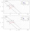 |
Fig. 6. Lens system configurations for the close and wide 2L2S solutions of KMT-2018-BLG-2119. Notations are the same as those in Fig. 3. |
4. Source stars and Einstein radii
In this section, we specify the source stars of the events for the estimation of the angular Einstein radii as well as for the full characterization of the events. We specify the source of each event by measuring the extinction- and reddening-corrected (dereddened) color and magnitude using the Yoo et al. (2004) routine. In this routine, the source location in the instrumental CMD of neighboring stars around the source is first determined by measuring the instrumental magnitudes of the source in two passbands, IS and VS, and then the source color and magnitude, (V − I, I)S, are calibrated using the red giant clump (RGC) centroid, with the instrumental color and magnitude of (V − I, I)RGC, in the CMD. The RGC centroid is used as a reference for calibration because its dereddened color and magnitude, (V − I, I)RGC, 0, are known (Bensby et al. 2013; Nataf et al. 2013).
Figure 7 shows the source locations of the two events in the instrumental CMDs constructed with the KMTC data sets that were processed using the pyDIA code. For each event, we first measured the combined magnitudes of the source IS and VS with the flux values of FS, I and FS, V, respectively, by regressing the pyDIA light curve data measured in the individual passbands with respect to the flux predicted by the model of
![$$ \begin{aligned} F_{\rm p}(t) = F_{\rm S,p} [A_1(t) + q_{\rm F,p} A_2(t)] + F_{\rm b,p}. \end{aligned} $$](/articles/aa/full_html/2023/02/aa45525-22/aa45525-22-eq4.gif)
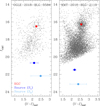 |
Fig. 7. Locations of the binary source stars in the instrumental color–magnitude diagrams. In each panel, the blue and cyan dots represent the locations of the primary (S1 and S2) and secondary source stars, resprectively, and the red dot denotes the centroids of red giant clump (RGC). |
Here A1(t) and A2(t) represent the lensing magnifications involved with the primary and secondary source stars, respectively; FS, p is the combined flux from the two source stars; Fb, p represents the blended flux from nearby unresolved stars; and the subscript “p” denotes the observation passband, that is, I and V. With the measured FS, p, we then estimated the flux values of the individual source components S1 and S2 using the relations
where FS, p = FS1, p + FS2, p. The V-band flux ratios, which are qF, V = 0.18 ± 0.15 for KMT-2018-BLG-0584 and qF, V = 0.18 ± 0.09 for KMT-2018-BLG-2119, were measured from the additional modeling conducted with the inclusion of the V-band data of the individual events. The instrumental color and magnitude were then calibrated by (V − I, I)0 = (V − I, I)RGC, 0 + Δ(V − I, I), where Δ(V − I, I) = (V − I, I)S − (V − I)RGC denotes the color and magnitude offsets of the source from the RGC centroid.
In Table 5, we list the values of (V − I, I)S, (V − I, I)RGC, (V − I, I)RGC, 0, and (V − I, I)S, 0 of the stars comprising the binary sources of the two events. According to the estimated colors and magnitudes, the source of OGLE-2018-BLG-0584 is a binary composed of two K-type dwarfs, and the source of KMT-2018-BLG-2119 is a binary composed of two dwarfs of G and K spectral types.
Source colors, magnitudes, angular radii, Einstein radii, and relative proper motion.
With the estimated source color and magnitude, the angular Einstein radius was estimated from the relation

where the angular radius of the source star, θ*, was deduced from the dereddened color and magnitude and the normalized source radius was obtained from modeling. For the estimation of θ*, we first converted the V − I color into the V − K color using the Bessell & Brett (1988) relation and then deduced θ* from the Kervella et al. (2004) relation between (V − K, V) and θ*. With the measured Einstein radius, the relative lens-source proper motion was estimated from θE and tE by

The estimated values of θ*, θE, and μ are presented in Table 5. In the table, we list two sets of (θ*, θE, μ) values. In one set, the values are based on the color and magnitude of the primary source S1 (the values presented in the column with the heading “S1”), and in the other set, the values are based on those of the secondary source S2 (in the column with the heading “S2”). We found that the values θE and μ estimated from S1 and S2 are consistent, giving more credibility to the 2L2S interpretations of the events.
We note that the estimated lens-source proper motion of OGLE-2018-BLG-0584, μ ≳ 12.2 mas yr−1, is substantially bigger than ∼5 mas yr−1 of typical lensing events. The lens of this event can be resolved from the source in about ten years by high angular resolution observations with 8 m class telescopes or the Hubble Space Telescope, as in the case of the planetary event OGLE-2005-BLG-169 (Batista et al. 2015; Bennett et al. 2015). The lens luminosity measurement from this high resolution image will be useful not only to confirm the 2L2S interpretation but also to constrain the physical lens parameters. For potential follow-up observations in the future, we estimate that the K-band magnitude of the combined source stars would be K ∼ 17.5.
5. Physical lens parameters
In this section, we estimate the physical parameters of the lens systems, including the mass and distance. These parameters can be uniquely determined by measuring the extra lensing observables of the microlens parallax πE and Einstein radius by
where  , πS = AU/DS, and DS denotes the distance to the source. For both OGLE-2018-BLG-0584 and KMT-2018-BLG-2119 events, the Einstein radii were measured, but the values of the microlens parallax could not be securely measured for either of the events. We therefore estimated M and DL by conducting Bayesian analyses based on the measured observables of tE and θE, which are related to the physical parameters by
respectively. Here πrel = AU(1/DL − 1/DS) denotes the relative lens-source parallax.
The Bayesian analysis of each lensing event was conducted by producing a large number of artificial events. For the individual artificial events, the locations and velocities of the lenses and source stars were derived from a Galactic model, and the masses of the lenses were derived from a model mass function by conducting a Monte Carlo simulation. In the simulation, we adopted the Galactic model and mass function described in detail by Jung et al. (2021). We then constructed the posteriors of M and DL by imposing a weight of wi = exp(−χ2/2) to each simulated event. Here, the χ2 value is computed by
![$$ \begin{aligned} \chi ^2 = {(t_{\mathrm{E},i} - t_{\rm E})^2 \over [\sigma (t_{\rm E})]^2} + {(\theta _{\mathrm{E},i} - \theta _{\rm E})^2 \over [\sigma (\theta _{\rm E})]^2}, \end{aligned} $$](/articles/aa/full_html/2023/02/aa45525-22/aa45525-22-eq11.gif)
where (tE, i, θE, i) denote the event timescale and Einstein radius of each simulated lensing event computed from the relations in Eq. (6), (tE, θE) indicate the measured values, and [σ(tE),σ(θE)] represent their measurement uncertainties. In our analyses, we use the values of θE estimated from the colors and magnitudes of the primary source stars.
The posteriors of the mass of the primary lens and distance to the lens systems constructed from the Bayesian analyses for the OGLE-2018-BLG-0584 and KMT-2018-BLG-2119 events are presented in Figs. 8 and 9, respectively. In each panel, we represent the distributions obtained based on the close and wide solutions. The distribution of the source distance DS in the bottom panel of each figure is presented to show the relative locations of the lens and source.
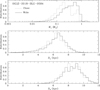 |
Fig. 8. Bayesian posteriors of primary lens mass, distance to lens, and source for the lensing event OGLE-2018-BLG-0584. Dotted and solid curves are based on the close and wide solutions, respectively. |
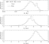 |
Fig. 9. Bayesian posteriors of physical lens parameters for KMT-2018-BLG-2119. Notations are the same as those in Fig. 8. |
In Table 6, we list the Bayesian estimates of the primary and secondary lens masses, M1 and M2; distance, DL; and projected separation, a⊥, between the lens components for the individual events. The projected separation is computed from the binary separation, angular Einstein radius, and lens distance by a⊥ = sDLθE. The upper and lower limits of the individual lens parameters are set as the 16% and 84% ranges of the posterior distributions. We note that there are some variations in the parameters depending on the close and wide solutions of the events. Nevertheless, the estimated parameters indicate that the lens of OGLE-2018-BLG-0584 is a binary composed of two M dwarfs and that the lens of KMT-2018-BLG-2119 is a binary composed of a low-mass M dwarf and a brown dwarf. The detection of the brown dwarf companion of KMT-2018-BLG-2119L demonstrates the usefulness of binary lens events in detecting microlensing brown dwarfs, as recently illustrated by Han et al. (2022c,e).
Physical lens parameters.
6. Summary
We re-investigated the two lensing events OGLE-2018-BLG-0584 and KMT-2018-BLG-2119, as there had been no suggested models explaining the anomalies in their lensing light curves. We found that the light curves could not be explained by the usual models based on either a 2L1S or a 1L2S interpretation.
We re-analyzed the light curves of the events with more sophisticated models that included an extra lens or a source component to the 2L1S lens system configuration. From our analyses, we found that a 2L2S interpretation explains the light curves of both events well and that for each event there exists a pair of solutions resulting from the close–wide degeneracy.
The two events studied in this paper are the sixth and seventh events for which both the lens and source are identified as binaries. For the event OGLE-2018-BLG-0584, the source is a binary composed of two K-type stars and the lens is a binary composed of two M dwarfs. For the event KMT-2018-BLG-2119, the source is a binary composed of two dwarfs of G and K spectral types and the lens is a binary composed of a low-mass M dwarf and a brown dwarf.
For example, the lensing event model page maintained by Cheongho Han (http://astroph.chungbuk.ac.kr/~cheongho).
Acknowledgments
Work by C.H. was supported by the grants of National Research Foundation of Korea (2020R1A4A2002885 and 2019R1A2C2085965). J.C.Y. acknowledges support from U.S. NSF Grant No. AST-2108414. Y.S. acknowledges support from BSF Grant No. 2020740. This research has made use of the KMTNet system operated by the Korea Astronomy and Space Science Institute (KASI) and the data were obtained at three host sites of CTIO in Chile, SAAO in South Africa, and SSO in Australia.
References
- Albrow, M. 2017, https://doi.org/10.5281/zenodo.268049 [Google Scholar]
- Albrow, M., Horne, K., Bramich, D. M., et al. 2009, MNRAS, 397, 2099 [Google Scholar]
- Aubourg, E., Bareyre, P., Bréhin, S., et al. 1993, Nature, 365, 623 [NASA ADS] [CrossRef] [Google Scholar]
- Alcock, C., Akerlof, C. W., Allsman, R. A., et al. 1993, Nature, 365, 621 [NASA ADS] [CrossRef] [Google Scholar]
- An, J. H. 2005, MNRAS, 356, 1409 [Google Scholar]
- Batista, V., Beaulieu, J.-P., Bennett, D. P., et al. 2015, ApJ, 808, 170 [Google Scholar]
- Beaulieu, J.-P., Bennett, D. P., Batista, V., et al. 2016, ApJ, 824, 83 [CrossRef] [Google Scholar]
- Bennett, D. P., & Rhie, S. H. 1996, ApJ, 472, 660 [NASA ADS] [CrossRef] [Google Scholar]
- Bennett, D. P., Rhie, S. H., Nikolaev, S., et al. 2010, ApJ, 713, 837 [Google Scholar]
- Bennett, D. P., Bhattacharya, A., Anderson, J., et al. 2015, ApJ, 808, 169 [Google Scholar]
- Bennett, D. P., Rhie, S. H., Udalski, A., et al. 2016, AJ, 152, 125 [Google Scholar]
- Bennett, D. P., Udalski, A., Han, C., et al. 2018, AJ, 155, 141 [Google Scholar]
- Bennett, D. P., Udalski, A., Bond, I. A., et al. 2020, AJ, 160, 72 [NASA ADS] [CrossRef] [Google Scholar]
- Bond, I. A., Abe, F., Dodd, R. J., et al. 2001, MNRAS, 327, 868 [Google Scholar]
- Bensby, T., Yee, J. C., Feltzing, S., et al. 2013, A&A, 549, A147 [NASA ADS] [CrossRef] [EDP Sciences] [Google Scholar]
- Bessell, M. S., & Brett, J. M. 1988, PASP, 100, 1134 [Google Scholar]
- Bozza, V. 1999, A&A, 348, 311 [NASA ADS] [Google Scholar]
- Daněk, K., & Heyrovský, D. 2015a, ApJ, 806, 63 [CrossRef] [Google Scholar]
- Daněk, K., & Heyrovský, D. 2015b, ApJ, 806, 99 [CrossRef] [Google Scholar]
- Daněk, K., & Heyrovský, D. 2019, ApJ, 880, 72 [CrossRef] [Google Scholar]
- Dominik, M. 1999, A&A, 349, 108 [NASA ADS] [Google Scholar]
- Gaudi, B. S., Naber, R. M., & Sackett, P. D. 1998, ApJ, 502, L33 [CrossRef] [Google Scholar]
- Gaudi, B. S., Bennett, D. P., Udalski, A., et al. 2008, Science, 319, 927 [Google Scholar]
- Griest, K., & Hu, W. 1993, ApJ, 407, 440 [NASA ADS] [CrossRef] [Google Scholar]
- Han, C., & Gould, A. 1997, ApJ, 480, 196 [NASA ADS] [CrossRef] [Google Scholar]
- Han, C., & Gould, A. 2003, ApJ, 592, 172 [Google Scholar]
- Han, C., Chang, H.-Y., An, J. H., & Chang, K. 2001, MNRAS, 328, 986 [NASA ADS] [CrossRef] [Google Scholar]
- Han, C., Udalski, A., Choi, J.-Y., et al. 2013, ApJ, 762, L28 [Google Scholar]
- Han, C., Udalski, A., Gould, A., et al. 2017, AJ, 154, 223 [Google Scholar]
- Han, C., Bennett, D. P., Udalski, A., et al. 2019, AJ, 158, 114 [Google Scholar]
- Han, C., Lee, C.-U., Udalski, A., et al. 2020, AJ, 159, 48 [Google Scholar]
- Han, C., Albrow, M. D., Chung, S.-J., et al. 2021a, A&A, 652, A145 [NASA ADS] [CrossRef] [EDP Sciences] [Google Scholar]
- Han, C., Lee, C.-U., Ryu, Y.-H., et al. 2021b, A&A, 649, A91 [NASA ADS] [CrossRef] [EDP Sciences] [Google Scholar]
- Han, C., Udalski, A., Kim, D., et al. 2021c, AJ, 161, 270 [NASA ADS] [CrossRef] [Google Scholar]
- Han, C., Gould, A., Bond, I. A., et al. 2022a, A&A, 662, A70 [NASA ADS] [CrossRef] [EDP Sciences] [Google Scholar]
- Han, C., Gould, A., Kim, D., et al. 2022b, A&A, 663, A145 [NASA ADS] [CrossRef] [EDP Sciences] [Google Scholar]
- Han, C., Jung, Y. K., Kim, D., et al. 2022c, A&A, submitted [Google Scholar]
- Han, C., Kim, D., Yang, H., et al. 2022d, A&A, 662, A70 [NASA ADS] [CrossRef] [EDP Sciences] [Google Scholar]
- Han, C., Ryu, Y.-H., Shin, I.-G., et al. 2022e, A&A, 667, A64 [NASA ADS] [CrossRef] [EDP Sciences] [Google Scholar]
- Han, C., Udalski, A., & Lee, C.-U. 2022f, A&A, 658, A93 [NASA ADS] [CrossRef] [EDP Sciences] [Google Scholar]
- Han, C., Jung, Y. K., Gould, A., et al. 2023, A&A, in press https://doi.org/10.1051/0004-6361/202245644 [Google Scholar]
- Hwang, K.-H., Choi, J.-Y., Bond, I. A., et al. 2013, ApJ, 778, 55 [Google Scholar]
- Jung, Y. K., Udalski, A., Bond, I. A., et al. 2017, ApJ, 841, 75 [Google Scholar]
- Jung, Y. K., Han, C., Udalski, A., et al. 2021, AJ, 161, 293 [NASA ADS] [CrossRef] [Google Scholar]
- Kervella, P., Thévenin, F., Di Folco, E., & Ségransan, D. 2004, A&A, 426, 29 [Google Scholar]
- Kim, S.-L., Lee, C.-U., Park, B.-G., et al. 2016, J. Korean Astron. Soc., 49, 37 [Google Scholar]
- Kim, D.-J., Kim, H.-W., Hwang, K.-H., et al. 2018a, AJ, 155, 76 [Google Scholar]
- Kim, H. W., Hwang, K. H., Shvartzvald, Y., et al. 2018b, AAS, submitted [arXiv:1806.07545] [Google Scholar]
- Mao, S., & Paczyński, B. 1991, ApJ, 374, L37 [Google Scholar]
- Nataf, D. M., Gould, A., Fouqué, P., et al. 2013, ApJ, 769, 88 [Google Scholar]
- Paczyński, B. 1986, ApJ, 301, 503 [NASA ADS] [CrossRef] [Google Scholar]
- Poleski, R., Skowron, J., Udalski, A., et al. 2014, ApJ, 795, 42 [Google Scholar]
- Udalski, A. 2003, Acta Astron., 53, 291 [NASA ADS] [Google Scholar]
- Udalski, A., Szymański, M., Kałużny, J., et al. 1994, Acta Astron., 44, 1 [Google Scholar]
- Udalski, A., Szymański, M. K., & Szymański, G. 2015, Acta Astron., 65, 1 [NASA ADS] [Google Scholar]
- Yee, J. C., Shvartzvald, Y., Gal-Yam, A., et al. 2012, ApJ, 755, 102 [Google Scholar]
- Yoo, J., DePoy, D. L., Gal-Yam, A., et al. 2004, ApJ, 603, 139 [Google Scholar]
- Zang, W., Han, C., Kondo, I., et al. 2021, RAA, 21, 239 [NASA ADS] [Google Scholar]
All Tables
Source colors, magnitudes, angular radii, Einstein radii, and relative proper motion.
All Figures
|
Fig. 1. Light curve of OGLE-2018-BLG-0584. The curve drawn over the data points is the model of the close 2L1S solution found from the fit of the data excluding those in the region 8224.5 ≤ HJD − 2450000 ≤ 8225.5. The upper panel shows the zoom of the anomaly region. |
| In the text | |
|
Fig. 2. Comparisons of models in anomaly region of OGLE-2018-BLG-0584 light curve. The top panel shows the four models of the close and wide 2L2S, 3L1S, and 2L1S solutions, and the lower panels show the residuals from the individual models. The three insets in the top panel show the lens system configurations of the 2L1S and 3L1S solutions. In each inset, the red figures represent the caustics and the line with an arrow indicates the source trajectory. The configuration of the 2L2S solutions are presented in Fig. 3. |
| In the text | |
|
Fig. 3. Lens system configurations for the close (upper panel) and wide (lower panel) 2L2S solutions of OGLE-2018-BLG-0584. In each panel, the close figure represents the caustic, and the two lines with arrows marked by S1 and S2 represent the trajectories of the primary (S1) and secondary (S2) source stars. The grey curves encompassing the caustic represent the equimagnification contours. The inset in each panel shows the whole view of the lens system, where the blue dots represent the positions of the binary lens components and the dotted circle is the Einstein ring. |
| In the text | |
|
Fig. 4. Light curve of KMT-2018-BLG-2119. The curve drawn over the data points is a 2L1S model (close solution) obtained by fitting the light curve with the exclusion of the data in the region of 8380.7 ≤ HJD′≤8384.0. |
| In the text | |
|
Fig. 5. Comparison of models in the anomaly region of the KMT-2018-BLG-2119 light curve. Notations are the same as those in Fig. 2. |
| In the text | |
|
Fig. 6. Lens system configurations for the close and wide 2L2S solutions of KMT-2018-BLG-2119. Notations are the same as those in Fig. 3. |
| In the text | |
|
Fig. 7. Locations of the binary source stars in the instrumental color–magnitude diagrams. In each panel, the blue and cyan dots represent the locations of the primary (S1 and S2) and secondary source stars, resprectively, and the red dot denotes the centroids of red giant clump (RGC). |
| In the text | |
|
Fig. 8. Bayesian posteriors of primary lens mass, distance to lens, and source for the lensing event OGLE-2018-BLG-0584. Dotted and solid curves are based on the close and wide solutions, respectively. |
| In the text | |
|
Fig. 9. Bayesian posteriors of physical lens parameters for KMT-2018-BLG-2119. Notations are the same as those in Fig. 8. |
| In the text | |
Current usage metrics show cumulative count of Article Views (full-text article views including HTML views, PDF and ePub downloads, according to the available data) and Abstracts Views on Vision4Press platform.
Data correspond to usage on the plateform after 2015. The current usage metrics is available 48-96 hours after online publication and is updated daily on week days.
Initial download of the metrics may take a while.