| Issue |
A&A
Volume 662, June 2022
|
|
|---|---|---|
| Article Number | A99 | |
| Number of page(s) | 29 | |
| Section | Planets and planetary systems | |
| DOI | https://doi.org/10.1051/0004-6361/202142652 | |
| Published online | 24 June 2022 | |
Feasibility of detecting and characterizing embedded low-mass giant planets in gaps in the VIS/NIR wavelength range
University of Kiel, Institute of Theoretical Physics and Astrophysics,
Leibnizstrasse 15,
24118
Kiel, Germany
e-mail: This email address is being protected from spambots. You need JavaScript enabled to view it.
Received:
12
November
2021
Accepted:
1
February
2022
Abstract
High-contrast imaging in the visible and near-infrared (VIS/NIR) has revealed the presence of a plethora of substructures in circumstellar disks (CSDs). One of the most commonly observed substructures are concentric gaps that are often attributed to the presence of embedded forming planets. However, direct detections of these planets are extremely rare, and thus ambiguity regarding the origin of most gap features remains. The aim of this study is to investigate the capabilities of high-contrast VIS/NIR imaging of directly detecting and characterizing low-mass giant planets in gaps in a broad systematic parameter study. To this end, a grid of models of protoplanetary disks was generated. The models include a central T Tauri star surrounded by a face-on CSD harboring an accreting planet, which itself is surrounded by a circumplanetary disk (CPD) and carves a gap. These gaps are modeled using empirically determined profiles, and the whole system is simulated fully self-consistently using the Monte Carlo radiative transfer code Mol3D in order to generate temperature distributions and synthetic observations assuming a generic dust composition consisting of astronomical silicate and graphite. Based on these simulations, we measured the impact the planet and its CPD have on contrast curves and quantified the impact of the observing wavelength and of five key parameters (planetary mass, mass accretion rate, distance to the star, mass of the CPD, and mass of the CSD) on the determined signal strength. Subsequently, we applied a detection criterion on our results and assess the capabilities of the instrument SPHERE/VLT of detecting the embedded planets. We find that a part of the investigated parameter space includes detectable planets, and we elaborate on the implication a non-detection has on the underlying parameters of a potential planet and its CPD. Furthermore, we analyze the potential loss of valuable information that would enable the detection of embedded planets by the use of a coronagraphic mask. However, we find this outcome to be extremely unlikely in the case of SPHERE. Finally, within the VIS/NIR wavelength range we identify for each of the investigated basic properties of the planets and the disks the most promising observing wavelengths that enable us to distinguish between different underlying parameter values. In doing so, we find that the detectability and the characterization often benefit from different observing wavelengths, highlighting the complementarity and importance of multiwavelength observations.
Key words: methods: numerical / protoplanetary disks / radiative transfer / planets and satellites: detection / planets and satellites: fundamental parameters / infrared: planetary systems
© ESO 2022
1 Introduction
In recent years, the quest to observe embedded accreting planets as they form has come a long way as a result of combined observations that are covering the ultraviolet to the millimeter wavelength ranges. One instrument in particular has been playing a major role in this, due to its diffraction-limited and high-contrast observations: the Spectro-Polarimetric High contrast imager for Exoplanets REsearch (SPHERE; Beuzit et al. 2019), which covers the visible and near-infrared (VIS/NIR) wavelength ranges. Together with other instruments, it has revealed a large abundance of substructures that are now known to be commonly present in protoplanetary disks (PPDs) ranging from gaps and rings to spiral arms, cavities, and various asymmetric features (e.g., Garufi et al. 2016, 2018; Avenhaus et al. 2018; Andrews et al. 2018, DSHARP). These features are often interpreted as the result of embedded planets that interact with their natal circumstellar disk (CSD; e.g., Wolf & D’Angelo 2005; Fouchet et al. 2010; Ruge et al. 2013; Ober et al. 2015; Dong et al. 2016). However, other origins have been proposed as well (e.g., Flock et al. 2015; Zhang et al. 2015; Ruge et al. 2016; Gonzalez et al. 2017; Suriano et al. 2017, 2019; Dullemond & Penzlin 2018). Despite the ambiguity of their particular origins, the properties of the potential planets that may produce these features have been studied extensively, especially using hydrodynamics simulations (e.g., Bae et al. 2019; Toci et al. 2020; Calcino et al. 2020). Dong & Fung (2017), for instance, analyzed observed gap features in order to determine the masses of planets that may have caused them by using 2D and 3D hydrodynamics simulations with 3D radiative transfer simulations of five scattered light observations of CSDs around Herbig Ae/Be and T Tauri stars: HD 97048 (Ginski et al. 2016), TW Hya (van Boekel et al. 2017), HD 169142 (Momose et al. 2015), LkCa15 (Thalmann et al. 2016), and RX J1615 (de Boer et al. 2016). By assuming an α-viscosity model (Shakura & Sunyaev 1973) with αvisc = 10−3 and single gap-opening planets as origins, they deduced that the corresponding planetary masses are all of typical low-mass giant planets between about 0.1 and 1 MJ.
While the kinematic detection of a planet has proven to be very useful (Pinte et al. 2018, 2019), in order to avoid much of the ambiguity that is present in the analysis of indirect features it is highly desirable to directly image the embedded planets. Unfortunately, this task is extremely challenging and observations are still rare. To date, the only two thus confirmed embedded planets, PDS 70 b and PDS 70 c, are both located around PDS 70 (Keppler et al. 2018; Müller et al. 2018; Haffert et al. 2019; Mesa et al. 2019), in which case it was even possible to restrict the basic parameters of potential circumplanetary disks (CPDs) surrounding both of them (Isella et al. 2019; Benisty et al. 2021).
In this study, we focus on systems of low-mass giant planets carving gaps into the CSDs of T Tauri stars in which the planets themselves are surrounded by their own CPDs characterized by their accretion luminosity. Our goal is to assess the potential for direct detections and for the characterization of these planets and their CPDs in the VIS/NIR wavelength range in a systematic manner. Studying this particular class of planets is important as they are likely much more prevalent than their more massive counterparts; the overall occurrence rate of 5 to 13 MJ companions located at orbital distances of 30 to 300 au is only  in systems with stellar masses of 0.1 to 3 M⊙ (Bowler 2016). Therefore, we generated models of these systems and made use of the gap profiles that were empirically determined by Kanagawa et al. (2016, 2017) and subsequently improved (Gyeol Yun et al. 2019). We then conducted a broad parameter study by performing fully self-consistent Monte Carlo radiative transfer (MCRT) simulations based on these models using the code Mol3D (Ober et al. 2015). The code was equipped with a method for dealing with the extremely high optical depths encountered in CPDs (Krieger & Wolf 2020) in order to significantly reduce noise in the determined temperature distributions and flux maps and, thus, improve the reliability of our simulations.
We then use the generated synthetic observations to assess the relevance of the different sources of flux observed in the VIS/NIR when trying to directly detect planets and their CPDs. Here we particularly elaborate on the relevance of proper simulations of thermal self-scattered flux of the CPDs as this turns out to be of high importance for this purpose. We generated convolved radial contrast profiles and quantified the impact of the planet and CPD on observations for each model at different observing wavelengths. The particular method that we used to measure the impact requires a conversion of the Cartesian detector grid to a polar detector grid, for which we present for this purpose the specifically written python package CartToPolarDetector1. The obtained contrast values that measure the impact were then used as a basis for studying the detectability and “characterizability” of embedded planets and their CPDs with respect to the various underlying parameters of the model. With a particular focus on observing modes possible with SPHERE, we then discuss the possibility of losing valuable information due to the use of a coronagraph as a result of an inner working angle that is too small. And last, we deduce observing wavelengths that are best suited for detecting planets and CPDs and for characterizing their various basic properties in the VIS/NIR wavelength range.
The paper is structured as follows. In Sect. 2, the model setup and methods to reliably perform MCRT simulations are described. Instruments that are analyzed later on are listed in Sect. 2.4. Subsequently, Sect. 3 presents the method we use to measure the impact of embedded planets and their CPDs on observations, and discuss the detectability and characterizability of these planets and their CPDs. Finally, Sect. 4 presents a summary of our results and conclusions regarding observations with SPHERE and future instruments.
2 Setup and methods
This study is performed on the basis of PPD models that are analyzed by the use of MCRT simulations and then evaluated with regard to the detectability and characterization of their embedded protoplanets. In this section, we lay the foundation for the study by briefly summarizing the core principles of MCRT simulations and describing the components that constitute the models.
2.1 MCRT
In this study we perform MCRT simulations based on the code Mol3D (Ober et al. 2015). Given a density distribution of dust and gas and a list of sources for radiation, Mol3D simulates the path and interactions of emitted photon packages individually and randomly according to their corresponding probability distributions. To this end, the model space is described by a grid whose cells have homogeneous and constant physical properties (e.g., density and temperature) in which the various sources are placed. This eventually allows a precise temperature distribution to be determined as well as wavelength-dependent flux maps (i.e., synthetic observations) to be produced. The high level of computational performance that is required to properly simulate complex systems is achieved by utilizing a method of locally divergence-free continuous absorption of photon packages (Lucy 1999) together with an immediate reemission scheme according to a temperature-corrected spectrum (Bjorkman & Wood 2001) and a method that utilizes a large database of precalculated photon paths in optically thick dusty media (Krieger & Wolf 2020).
2.2 Setup
In the following we describe the simulated models in terms of their structural components as well as the instruments and corresponding wavelengths that we studied. In general, the setup is composed of a star that is located in the center of a CSD, which harbors an accreting planet that itself is embedded in a CPD and carves a gap into the CSD. A list of the model parameters used can be found in Table 1.
2.2.1 Stellarand CSD model
The star and the planet are implemented as point sources, described by a blackbody spectrum corresponding to their assigned effective temperatures and radii, which are surrounded by their corresponding disks. The effective temperature of the star and its radius are given by T* and R*, respectively, and the star is located at a distance d from the observer. In this study we apply a disk model that is described by a three-dimensional parameterized density distribution given by
 (1)
(1)
where r is the distance to its corresponding central object n in the direction perpendicular to the z-axis, and Σn(r) and hn(r) are the surface density distribution and scale height of the disk, respectively. For the description of the CSD we use the subscript n = s where s is referring to the star. In this case the surface density distribution and scale height are given by
 (2)
(2)
and
 (3)
(3)
respectively, which is based on the description of Lynden-Bell & Pringle (1974) and Hartmann et al. (1998); however, the CSD density distribution is additionally adapted for the purpose of modeling a gap that arises due to the presence of an embedded accreting planet. In general, the parameters αn and βn describe the compactness and the flaring of the disk around the central object n, respectively; Σ0; n and h0; n describe the corresponding surface density and scale height evaluated at the reference radius r0; n, respectively; and rin; n is the inner and rout; n the outer radius of the disk. For most model parameters we chose commonly used values constrained from observations of CSDs around T Tauri stars (e.g., DSHARP; Andrews et al. 2009; Galli et al. 2015). Additionally, the surface density is perturbed by an accreting planet, which carves a gap into the disk, whose surface density profile is described by  . The gap profile is based on an empirically determined (Kanagawa et al. 2016, 2017) and later improved (Gyeol Yun et al. 2019) model that is given by
 (4)
(4)
with
 (5)
(5)
 (6)
(6)
 (7)
(7)
 (8)
(8)
and hp = hs(rp). Here, rp, Mp, and hp are the radius of the planetary orbit, the mass of the planet, and the scale height of the CSD at the position of the planet, respectively. In addition, M* is the mass of the central star and αvisc the parameter of the α-viscosity model (Shakura & Sunyaev 1973). The gap profile is azimuthally symmetric with the planet marking the center of a plateau (|r − rp| < ∆r1), where the profile reaches its minimal value  as can be seen in Eq. (4). Outside of this minimum, the gap profile increases linearly in the radial direction until it reaches a value of 1 at |r − rp| = ∆r2, as described by Eq. (5). Outside the gap region (i.e., at |r − rp| > ∆r2) the CSD is unperturbed by the planetary gravitational impact. The quantities ∆r1 and ∆r2 from Eq. (6) are thus half of the radial width of the gap plateau and half of the total radial width of the gap, respectively.
Collection of selected model parameters.
2.2.2 Planetary and CPD model
Similarly to the star, the planet is characterized by a point-source that is described by a blackbody spectrum. Since the planet is young and still accretes matter, its effective temperature is a combination of its intrinsic temperature and its accretion temperature.
The accretion temperature is linked via the Stefan-Boltzmann law to the accretion luminosity which itself is given by (e.g., Marleau et al. 2017, 2019)
 (9)
(9)
where G is the gravitational constant,  the mass accretion rate onto the planet, Rp the radius of the planet, and η the efficiency by which gravitational energy is converted into radiative energy as matter falls onto the planet. We note that the efficiency η in general depends on various quantities; however, for simplicity we assume the case of cold accretion (i.e., η = 1). In this study the parameter
  assumes two different values that correspond to a relatively low and a relatively high mass accretion rate with respect to the chosen part of the parameter space (see Table 1). The chosen values were estimated using the empirical results of Tanigawa & Tanaka (2016). The point-source approximation is justified since most of the accreted material is assumed to be accreted via the poles of the planet or in its radially close vicinity (Klahr & Kley 2006; Tanigawa et al. 2012).
Within the considered planetary mass range the intrinsic luminosity is expected to be given by roughly Lint = 10−5 L⊙ (see, e.g., Fig. 7 in Mordasini et al. 2017). However, by comparing the corresponding expected intrinsic temperature of the simulated planets with their accretion temperature, we find that the latter is strongly dominating. In particular, the resulting effective temperature of our simulated planets changes only by a few percent, and thus we neglect the contribution from the intrinsic luminosity in this study.
The density distribution of the CPD is defined in Eq. (1) and uses the subscript n = p. Its corresponding surface density and scale height are then given by
 (10)
(10)
and
 (11)
(11)
respectively. Contrary to the observation-based choice of CSD parameters, the CPD parameters are based on results of hydrodynamic simulations. While these parameters may differ in different simulations and studies, we tried to choose generic values for our models. The chosen parameters are αp = 2.5 (compare with Tanigawa et al. 2012; Szulágyi 2017), hout;p = hp(rout) = 0.5 rout (compare with Ayliffe & Bate 2009), and
 (12)
(12)
for the outer radius of the CPD (compare with Szulágyi 2017). The parameter βp is obtained via the relation α = 3 (β − 0.5) (Shakura & Sunyaev 1973). The parameter MCPD typically reaches a value of ~10−3 MJ for a Jupiter-mass planet (Szulágyi 2017) and is one of the parameters varied within this study. The reference radius for the CPD is chosen depending on the size of the Hill sphere in such a way that the density of the CPD reaches a value well below the ambient gap density to prevent abrupt density changes at the outer edge of the CPD. The exact values of these parameters can be found in Table 1.
The density distribution of the CPD is then added to the density distribution of the CSD and in a final step the region around the planet within its corresponding sublimation radius is cleared from all of its dust (i.e., the dust density is set to zero). However, the inner radius of the CPD rin;p, which is defined by the sublimation radius, has to be determined for each of the models individually before the actual MCRT simulations can be performed, which is described in Sect. 3.1. In total, we simulate 72 different models among which we vary rp (three values), Mp (three values),  (two values), MCPD (two values), and MCSD (two values). Each model is then analyzed at three different wavelengths λ, which eventually results in a total of 216 fully performed and subsequently analyzed simulations.
2.2.3 Dust model
While dust growth and settling of dust grains has a major impact on the grain size distribution close to the midplane of curcumstellar disks (e.g., Pinte et al. 2007, 2008; Madlener et al. 2012; Gräfe et al. 2013; Wolff et al. 2021), the disk layers traced in the VIS/NIR wavelength range are dominated by small interstellar medium-like dust grains (e.g., Wolf et al. 2003; Sauter & Wolf 2011).
For this reason, we assume spherical dust grains with radii a ranging from 5 nm to 250 nm that follow a grain size distribution  with grain size distribution exponent qg = −3.5 (Mathis et al. 1977). With a bulk densit y of ρbulk = 2.5 g cm−3, dust grains consist of fSi = 62.5% astronomical silicate and fGr = 37.5% graphite, for which we apply the 1/3 : 2/3 approximation (
 ; Draine & Malhotra 1993). The corresponding wavelength-dependent refractive indices of these components are obtained from Draine & Lee (1984), Laor & Draine (1993), and Weingartner & Draine (2001) and used to calculate corresponding cross-sections under the assumption of Mie theory by using the code miex (Wolf & Voshchinnikov 2004). In a final step, the mean optical properties of dust grains are computed (Wolf 2003). The ratio of gas to dust is set to the canonical value of 100:1.
2.3 Simulation grid
The model is embedded in a grid that is defined in spherical coordinates. It is centered around the star, has an inner radius rin; s defined by the sublimation radius of dust using a sublimation temperature of Tsubl = 1500 K, and an outer radius rout; s, which is chosen large enough to ensure that the density drops sufficiently and the disk becomes optically thin at large radii. For the purpose of this paper, two grid regions have been defined: a highly resolved region around the planet and a region of low resolution far away from the planet.
The high-resolution region centers around the planet and extends up to the Hill radius. Within this region, we use 61 cells in each of the directions r, θ, and ϕ. Due to the high resolution, the cells in the vicinity of the planet strongly resemble a Cartesian grid with flat cell borders. The planetary cell (i.e., the cell whose center corresponds to the center of the planet) has a cell width that is defined by the diameter of the planet, thus barely fitting the planet inside it. Along the three orthogonal axes, cell widths grow exponentially with a constant step-factor. Outside the high-resolution region, the cell widths are constant for both angular coordinates θ and ϕ and their respective widths are chosen such that they are larger than the widths of the adjacent cells in the high-resolution region. Combined, this results in 172 cells in the θ-direction and 174 cells in the ϕ-direction. Contrary to the linear sampling angular coordinates in the low-resolution region, we use a logarithmic sampling of cell borders in the r-direction. To this end, we first define a step factor for the low-resolution region of sf = 1.05, and determine a radial width of the innermost cell that is as close as possible to but lower than Δrin;s = 0.02 rin;s, which is done in such a way that ensures a smooth transition between the low- and high-resolution region in r-direction. We then increase the cell width in the r-direction exponentially, starting from the innermost cell close to the star and moving outward with the chosen constant step factor until the high-resolution region is reached. At large enough radii, even outside the highly resolved Hill sphere, the low-resolution region begins again. Here, cell widths also grow exponentially according to sf, thus ensuring a smooth transition from the high- to the low-resolution region. As a consequence, the number of cells in the r-direction depends on the position and size of the Hill sphere of the planet, and ranges from 319 to 344 cells among all simulations.
A consequence of setting up this specific grid structure is the abundance of irregularly shaped cells in regions where one coordinate has a fine sampling and another coordinate a coarse sampling, leading to very oblate and prolate cells. Unfortunately, such cells may pose a problem to MCRT simulations when placed in an optically thick region far away from any source of radiation. In these regions of the model space, photon package counts are relatively low, which leads to a poor representation of potential photon paths in these irregularly shaped cells. Consequently, the determined temperature suffers from a relatively high level of noise. While the noise does not significantly change the overall integrated flux of these regions, it unfortunately has an impact on their spectra.
Even though it is not possible to completely eliminate the noise, there are methods for reducing it significantly. It is possible to check the effectiveness of such a method by generating flux maps and simply verifying whether or not flux maps of pure thermal emission are noisy. The method we apply to overcome this issue is to overlay these particular regions of higher resolution outside the Hill sphere, which are regions of irregularly shaped cells, with a coarse grid. Next, we combine multiple adjacent irregularly shaped cells into groups of cells, such that the shape of the group is more regularly shaped. During the temperature calculation, whenever a photon package traverses a cell that belongs to such a cell group, the temperature of the whole group is increased equally and simultaneously. In particular, the deposited energy is distributed equally between all the dust grains present in the corresponding group of cells. In order to achieve this, we assign a weight to every member of a group of cells, which equals the ratio of dust grains the cell contains to the total number within the whole group, and distribute the deposited energy accordingly. To this end, we define the groups of cells as follows. In both angular directions, the coarse grid is linearly sampled with a cell width of ~1 deg. In the radial direction we use the same number of linearly sampled coarse grid cells. This particular definition has proven to result in a substantially reduced level of noise.
Instrument specifications.
2.4 Instruments
Detecting and characterizing embedded planets requires state-of-the-art instrumentation. In this study we particularly focus on two promising instruments that are installed on SPHERE: IRDIS and ZIMPOL. These instruments allow us to perform high-contrast observations in the VIS/NIR wavelength range using broadband filters in the classical imaging mode. Additionally, the use of a coronagraph further boosts their performance at detecting even comparably dim objects in the vicinity of a bright stars. To benefit from high planetary temperatures, we primarily focus on short observational wavelengths. Furthermore, we study the impact of the inner working angle (IWA) of coronagraphs on observations of close-in embedded planets. In particular, we measure the signal strength of simulated embedded planets that are hidden inside the IWA or located close to the its rim to assess the potential loss of detectable planets due to the application of a too small IWA. For this purpose, we simulate coronagraphs with the smallest possible IWA that are offered for their corresponding instruments and filters. Chosen instruments, modes, broadband filters, wavelengths, coronagraphs, and their corresponding IWAs are summarized in Table 2.
3 Results and discussion
In this section, we present the results of simulating embedded accreting planets, as described in Sect. 2.2. First, we present the findings regarding the determined inner radius of the CPD as well as its resulting temperature distribution. Then, we discuss resulting flux maps of all simulated systems regarding the relevance of their different sources of radiation. Subsequently, we describe a procedure with which we analyze all flux maps with respect to the detectability and characterization of the embedded planets and their CPDs. This method is applied and its results are used as a basis for discussing the relevance of different model parameters and deciding which SPHERE instrument, in terms of its observational wavelength, is best suited for characterizing which model parameter.
3.1 Determination of the CPD inner radius
As mentioned before, the inner radius rin;p is defined by the sublimation radius of dust in the vicinity of the planet (see Sect. 2.2.2). In general, its determination requires an iterative procedure that aims to narrow down the radius from both sides. On the one hand, the radius has to be large enough to eliminate the possibility of the onset of unexpected sublimation of dust during the run of a simulation. On the other hand, the radius has to be small enough to enable the dust to reach temperatures as close as possible to its sublimation temperature.
The temperature of any cell of the grid emerges as a consequence of exposure to direct or indirect stellar and planetary radiation. However, as expected at the sublimation radius of the planet we find that the contribution from the star is negligible compared to that of the planet. Therefore, during the determination of the inner radius of the CPD rin;p we only consider planetary radiation. Since MCRT simulations of highly optically thick regions are very time consuming and require the calculation of a high number of individual interactions per photon package, which in general should not be limited, we use Nγ = 105 photon packages per test run, which is the number of photon packages that were emitted from the planet to determine the resulting temperature distribution. For every test run we set a value for rin;p, beginning with the value rin;p = Rp, and calculate the resulting temperature distribution. Doing so, we are able to narrow down the value for rin;p from both sides. A value for rin;p is accepted, if (i) it did not result in the onset of unexpected sublimation during the test run, (ii) it is narrowed down to its actual value with an accuracy of <10% or ∆r < 1 Rp, and (iii) it is narrowed down to its actual value with an accuracy of ∆r < 2Rp. The reasoning for these criteria is as follows. The first criterion is generally required in any MCRT simulation of this type which determines equilibrium temperature distributions. The second and third criteria define relative and absolute levels of accuracy, respectively, with which rin; p has to be determined. However, since the grid has a finite resolution, the second criterion can also be satisfied if rin;p is determined down to the accuracy of the width of the planetary cell, which in terms of its volume is the smallest cell in the vicinity of the planet. It is worth mentioning that this method results in inner radii that may be rather slightly overestimated than underestimated, which is a direct consequence of the first mandatory criterion.
In general, the value of rin; p depends on the model parameters and needs to be determined individually for each simulation. However, we find that determining rin;p for models with a high value for MCSD first and then using the same sublimation radius for simulations with a lower value for MCSD, where all other underlying parameters coincide, is justified. In order to test the validity of this approach, we compare the maximum temperature of dust just outside the sublimation radius of all models, which only differ in their assumed parameter value of MCSD, and find that it differs by <3.3% for all simulations. This suggests only a weak dependence of rin;p on MCSD and affirms the viability of our approach. A list containing all determined inner radii rin; p can be found in Table C.1.
Dependence on rin;p. Results from Table C.1 suggest clear trends that describe the effect of different model parameters on rin;p. When keeping the remaining parameters constant, we find that rin;p increases if rp decreases, Mp increases,  increases, or MCPD increases. There are two underlying processes that can explain these trends. First, an increase in Lacc results in an extended sublimation radius. Second, an increased density at the inner rim of the CPD causes an enhanced back-warming effect, which leads to a larger sublimation radius. The effect can be described as follows. By increasing the density in the region behind the illuminated surface of the inner rim of the CPD, photons that cross that surface now have an increased probability of leaving the CPD through that same surface, as the probability of traveling through the already optically thick CPD and leaving it on the other side decreases. In a state of equilibrium this leads to an amplified radiation field at the illuminated surface of the inner rim of the CPD, and thus to an increased dust temperature. A more in-depth description of the back-warming effect including a one-dimensional derivation is presented in the Appendix A.
 |
Fig. 1 Temperature distribution in the midplane (left) and in a vertical cut through the midplane at the position of the planet (right) for a model with rp = 10 au, Mp = 1 MJ, |

3.2 Temperature distribution
Before the detectability of planets and their CPDs can be discussed, we determine the underlying temperature structure in a self-consistent manner. In order to do that for all models presented in Table 1, we set rin;p to the values deduced in the previous section and summarized in Table C.1. Additionally, we use rin;s = 0.07 au for all simulations. The dust emission properties of cells were precalculated for 501 logarithmically sampled temperature values between 2.7 and 3000 K and for 132 wavelenghts between 50 nm and 2 mm. For each model the temperature calculation is performed in two steps. In the first step, the star emits a total of Nγ = 108 photon packages, which increase the temperature in the whole model space. In the second step, the less luminous planet emits Nγ = 107 photon packages, which mainly leads to a significant change in the temperature distribution in the immediate vicinity of the planet. However, there are two exceptions made in the case of models with the lowest accretion luminosity Lacc and the greatest potential for high CPD densities (i.e., for the two models with the lowest values for Mp,  , and rp and the highest value for MCPD), where only Nγ = 106 photon packages are used in order to avoid very long simulation times. It was verified that these simulations, nonetheless, resulted in sufficiently smooth flux maps (see Sect. 2.3). Therefore, the reduced number of photon packages is not expected to reduce the quality of the results.
Figure 1 shows an example of the resulting temperature distribution for a model with rp = 10 au, Mp = 1MJ,  , MCPD = 0.1 × 10⁻³ MJ, and MCSD = 0.001 M⊙ in the midplane (left) as well as in a vertical cut through the midplane at the azimuthal position of the planet (right). The temperature distribution reaches its highest values in the vicinity of the star and the planet, and rapidly falls off at greater distances from the two objects. This temperature decrease is particularly strong in the region of the planet (i.e., in the CPD) effectively leading to a spatially confined impact of the planet on the temperature distribution. Moreover, the vertical cut shows a strong shadowing effect in the sense that the immediate planetary light is blocked by the CPD, and thus casts a shadow inside the gap, which keeps an otherwise hot region in the gap at a lower temperature. This effect is enhanced by the geometry of the CPD, which has an opening angle of ~90° (e.g., Szulágyi 2017), which is much wider than that of the CSD.
 |
Fig. 2 Flux maps at λ = 653 nm for a model with rp = 10 au, Mp = 1 MJ, |

3.3 Ideal observations
In order to determine the detectability of planets and their CPDs we have to calculate and evaluate flux maps for all models. There are different sources for radiation that constitute the total flux map detected by an observer: the star, the planet, and thermal radiation of dust. It is important to note that line emission may also play an important role in detecting embedded accreting planets; however, in this study we focus on the continuum emission of dust. In the case of thermal radiation, we additionally distinguish between unscattered radiation (Nsca = 0) and self-scattered radiation (Nsca ≥ 1). The latter is often understimated and omitted; however, we show that it is in general important in the case of embedded planets.
In order to determine the contribution of the different sources of radiation to the total flux map, all sources are calculated individually and their contributions are subsequently added up. For each model, wavelength, and radiation source the flux map is calculated individually, thus any declared number of photon packages refers to each of these flux maps individually. For the simulation of stellar and planetary radiation we use Nγ = 107 and Nγ = 106 photon packages, respectively. The unscattered thermal dust radiation is calculated with a ray-tracing algorithm that integrates and attenuates thermal dust radiation along the lines of sight in the direction of the detector. This method guarantees a smooth flux profile, but does not take into account self-scattering of thermal dust radiation. The process of self-scattering is simulated with Nγ = 108 photon packages that are distributed among all dust containing grid cells proportionally to their respective total luminosity, meaning that more luminous cells emit more photon packages. In addition, our method assures that every cell emits exactly its corresponding total luminosity.
Figure 2 shows examples of ideal flux maps for each of the four different sources at λ = 653 nm, which add up to the total flux of the model. Here, the model is described by rp = 10 au, Mp = 1MJ,  , MCPD = 0.1 × 10⁻³ MJ, and MCSD = 0.001 M⊙, and thus corresponds to the temperature distribution shown in Fig. 1. Every map consists of 1201 × 1201 pixels, each with a width of ~0.5 au, with the star located in the central pixel. The resulting flux map due to direct and scattered stellar light (upper left plot) shows some striking features: first, a peak of flux at the position of the star; second, an overall decline of flux toward greater radii; and third, the gap carved by the planet into the CSD. The planetary flux map (upper right plot) shows a strong peak at the position of the planet and a decline in flux toward greater distances from the planet, meaning that the signal is broadened due to the optical depth between the planet and the observer. The direct (i.e., unscattered) thermal radiation of dust (lower left plot) has its peak at the central pixel and quickly falls of toward larger radii. A second local maximum is reached at the position of the planet; however, its contribution is generally the weakest. The self-scattered radiation (lower right plot), which is composed of thermal dust radiation that has scattered at least once, reaches its highest value at the central pixel, overall falls off toward larger radii, has a bright ring just outside a clear gap, and shows a stronger signal at the position of the planet and its CPD than anywhere else inside the gap. Comparing the resulting contributions of these four sources we find that in the vicinity of the star scattered stellar light dominates the flux making all other contributions negligible. In the vicinity of the planet, however, stellar radiation, planetary radiation, and self-scattering of thermal dust radiation all play a crucial role. The contribution due to direct thermal radiation is comparably low in the considered wavelength range. Finally, it is important to note that in later sections we take into account the level of noise present across all flux maps in order to avoid overinterpreting any results with weak planetary and CPD signals.
For comparison purposes, Fig. 3 shows a cut of these flux maps along the x-axis. In particular, a stripe centered at the x-axis with a width of ∆y = 2RHill was averaged across the y-axis in order to reduce noise and better encompass the effect of the planet and the CPD. The plot clearly shows that despite the overall dominance of stellar flux, both the planetary radiation and the self-scattered thermal dust radiation may dominate the signal at the position of the planet. This emphasizes the need for a proper treatment of self-scattering in radiative transfer simulations in order to simulate embedded accreting planets.
Finally, Fig. 4 shows the total sum of all flux maps that are displayed individually in Fig. 2. It shows that for the most part the flux map is dominated by stellar radiation. There is also a very high contrast between the region around the star and the rest of the map, showing the need for methods that suppress the stellar contribution in order to directly detect a planet.
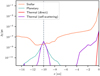 |
Fig. 3 Vertical cut through various flux maps at λ = 653 nm along the x-axis for a model with rp = 10 au, Mp = 1 MJ, |

3.4 Convolved observations
In order to systematically assess the expected strength of the signal of the combined system of planet and CPD, we perform the following steps. First, the total flux maps are convolved with a point-spread-function (PSF) that is defined by a Gaussian with a full width at half maximum given by FWHM = 1.22λ/D, with D = 8.2m as diameter2. Second, the Cartesian detector grid is converted to a polar detector grid in order to make use of the high degree of azimuthal symmetry of the observed PPD. Third, three regions are defined, namely an azimuthal region where the combined planetary and CPD signal is the strongest, a clearly defined gap region that is effectively free from any planetary and CPD signal, and a transition region connecting the azimuthal CPD and the azimuthal gap region. Finally, by subtracting the mean azimuthal gap radial profile from the mean azimuthal CPD radial profile we deduce the excess signal strength of the planet and its CPD3.
After an ideal (simulated) observation has been convolved using a wavelength-dependent beam size, a polar representation of the resulting map is constructed. The conversion of the Cartesian detector grid to a polar detector grid is performed with the python package CartToPolarDetector that was particularly written for this task. In order to find the polar representation of an originally Cartesian detector grid, the code overlays the Cartesian detector with a chosen polar grid and calculates the polar pixel values. Every Cartesian pixel is assumed to represent a homogeneous flux distribution across its full area. The associated value of a polar pixel is then the sum of all values of overlapping Cartesian pixels, each weighted with its geometrical intersection area with the polar pixel. Under the assumption of a homogeneous flux distribution within a Cartesian pixel, and since this approach does not rely on any method of interpolation, flux is conserved during the conversion. For the polar grid we choose Nϕ = 7200 and Nr = 3000 azimuthal and radial pixels, respectively, and place the center of the grid at the position of the star. This setup assures that the polar pixel area is smaller than the Cartesian pixel area in the vicinity of the planet, even in the case rp = 50 au, where the polar planetary pixel covers about half the area of the Cartesian planetary pixel. For more details regarding the python package, see Appendix B.
Next, we define three azimuthal regions. The azimuthal CPD region is defined as the smallest azimuthal interval that contains the full wavelength-dependent width of the beam in terms of its FWHM centered at the position of the planet, meaning that the radius that defines this region is given by
 (13)
(13)
Within this beam, the planetary pixel always has the highest absolute flux value within each simulation. Similar to the previous definition, the azimuthal gap region as well as the transition region is defined by a wavelength-dependent radius  in such a way that the contamination due to a planetary or CPD signal becomes insignificant outside this radius. In general, there are three different effects that have to be considered in order to determine
  , each extending the apparent spread of the planetary and CPD signal. There is, first, the spread due to the extended beam size
  ; second, the spread due to the optical depth between the planet and the observer
  ; and third, the spread due to the geometrical extent of the CPD
  . Apart from the third effect, which arises due to the geometrical extent of the area the signal originates from, the first two act on the signal solely by smearing it out radially. As a result,
  can be approximated as the sum of these radii given by
 (14)
(14)
The last contributor (i.e., the geometrical extent of the CPD) can be estimated based on the position and mass of the star and its companion. To mimic the situation of a real observation, where both the position and mass of an accreting planet are initially not known, we simply use an upper bound for the planetary mass, which in our case is given by 1MJ, and estimate  with the corresponding Hill radius as follows:
 (15)
(15)
Both of the other contributions are generally more difficult to estimate as they are wavelength-dependent and in general unconfined. However, an empirical analysis of our data shows that the relation presented in Eq. (16) is reliable for all models and wavelengths, as we make clear in later sections. As a result, we find that
 (16)
(16)
leads to a practically contamination-free azimuthal gap region in all simulations. We note that according to this definition, for any planet that is too close to the star, no contamination-free azimuthal gap region can be defined. In particular, the method can only be properly applied to systems that satisfy the condition
 (17)
(17)
Simulated SPHERE observations for long wavelengths and rp = 5 au, for instance, may not satisfy this condition (i.e., no clear gap signal can be deduced), which makes the determination of an excess planetary and CPD signal ambiguous. Nonetheless, even for these simulations we determine a signal, as discussed below. Finally, the azimuthal transition region is defined by  and
and  as the region that is neither part of the azimuthal CPD region nor of the azimuthal gap region.
The resulting ϕ interval that covers the azimuthal CPD region has an extent of
 (18)
(18)
In the case that the azimuthal gap region can be defined, it covers an angular extent of
 (19)
(19)
Figures 5 and 6 show radial profiles for two simulations at λ = 653 nm, whose parameters differ only in their values of rp.
The gray shaded area indicates the region in the plot where individual radial profiles that belong to one of the three azimuthal regions lie. The black curve is the mean radial profile of its corresponding azimuthal region. Additionally, each subplot highlights radial profiles that are located at the edges of their corresponding azimuthal regions and the left and right subplot also shows the central radial profile for the azimuthal gap and the azimuthal CPD region, respectively.
Both simulations show a distinct gap profile in their left plots. As expected, the gap depth is wider for the simulation with rp = 50 au compared to that with rp = 10 au. Even though they are not as smooth as the black mean curves, the light blue radial profiles (which indicate the border between the gap and the transition region) are not contaminated by planetary or CPD flux. Their level of statistical noise arises from the use of the Monte Carlo method and the limited number of simulated photon packages. Due to the definition of rtrans, the gap is practically free from any planetary or CPD flux. The gap region adjoins the transition region, which is shown in the middle plots. They clearly show an overall increase in flux going from the azimuthal gap region border (light blue curve) to the border of the azimuthal CPD region (orange curve), which was expected. The azimuthal CPD region is shown in the right plots, which features the strongest signal at the azimuthal and radial position of the planet inside the gap among all individual radial profiles in that azimuthal CPD region. In Fig. 5, however, the effect of the planet and its CPD is not strong enough to result in a local maximum at the position of the planet in the radial profile. Nonetheless, by comparison with the mean azimuthal gap profile, it becomes clear that the planet is indeed contributing strongly to the observed local flux value. Another interesting feature can be seen in the azimuthal gap region plot in Fig. 6, where a clear kink appears in the radial profile at ~ 10 au. This kink marks the transition where the contribution through stellar light, which is dominating the radial profile at small radii, becomes secondary to the contribution from the CSD and its embedded objects. In the next step we analyze the obtained mean radial profiles regarding the planetary and CPD signal strength, which leads into a discussion of the detectability and characterizability of embedded planets.
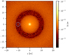 |
Fig. 4 Total flux map at λ = 653 nm for a model with rp = 10 au, Mp = 1 MJ, |

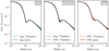 |
Fig. 5 Radial profiles at λ = 1.24 µm for a model with rp = 10 au, Mp = 1 MJ, |

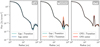 |
Fig. 6 Radial profiles at λ = 1.24 µm for a model with rp = 50 au, Mp = 1 MJ, |

3.5 Planetary and CPD signal strength
The purpose of this section is to describe the method with which the planetary and CPD signal strength as well as other detectable features are quantified, which lays the groundwork for the subsequent discussion on the detectability of embedded planets and the characterization of their properties. To this end, the shape of the mean radial profile of the azimuthal gap region as well as that of the azimuthal CPD region exhibit some common features that can be analyzed. The left plot in Fig. 7 shows a typical mean radial profile for the azimuthal gap region (gray curve) and, in addition, various relevant flux levels. As expected, the highest level of flux always originates from the position of the star at r = 0 au (gray solid line). As discussed in Sect. 2.4, we also simulate a coronagraph to study the impact of its inner working angle. In our simplified model of the coronagraph it acts on flux maps by reducing all incoming flux to zero within the full area of the IWA by granting unhindered transmission of flux outside of it. For the resulting exemplary observed radial profile (blue curve), we measure the flux level that is reached just outside the IWA of the coronagraph (short dashed line). If the radial profile features a gap, as can be seen in this plot, we also measure the minimum flux level inside the gap (dotted line) and the flux level of the adjacent ring (long dashed line), which is defined as the absolute maximum outside the gap region. In many simulations we find that no particular gap feature is present. This is usually the case, when the distance of the planet to the star is small and the observed wavelength relatively long. In this case, the aforementioned kink feature arises at a large radius and the stellar contribution, consequently, overlays any potential gap feature. However, we find that in this case the impact of an embedded planet shows mostly in a change of slope at the position of the kink, when comparing the mean radial profile of the azimuthal gap region with that of the azimuthal CPD region. Therefore, we identify those simulations and measure the level of flux at the kink, which is defined as an inflection point with a locally maximum positive change in slope.
Furthermore, to measure the impact of the planet and its CPD, we compute the contrast between the mean radial profile of the azimuthal gap region and the azimuthal CPD region, which is shown in the right plot in Fig. 7. To infer the correct radial position and magnitude of the planetary and CPD signal, even in the case of a weak signal, it is crucial to search for it in the correct radial range. In the case of simulations with rp = 50 au, this is done straightforwardly, since a clear plateau appears in the azimuthal gap profile between approximately rleft = 45 au and rright = 55 au. Here, rleft and rright denote the left and right border, respectively, of the interval within which the planetary and CPD signal is searched for, which itself is defined as the absolute maximum of the contrast profile in that interval.
In the case of rp ≤ 10 au we rely on a different method. If a gap feature is present, the gap depth is computed as the difference in flux between the gap and the ring. Next, the radial position of two points  and
and  are identified, where the gap reaches 50% of its depth. By definition, one of these points
  is to the left of the radial location of the gap minimum and one point
  is to the right. Using these points to define the search range for the planetary and CPD signal can potentially lead to false results, however. This is particularly the case if the gap is very shallow, which would often be accompanied by a very narrow search interval. To solve this issue, we introduce a minimum half interval length
  , which is the minimum distance the two interval borders individually need to be apart from the position of the gap minimum. We set
  , where rfeature is the radial position of the gap minimum. A review of all deduced planetary and CPD signals shows that this method results in a reliable identification of the planetary and CPD signal across all simulations and wavelengths. Furthermore, we also deduce a planetary and CPD signal in the absence of a gap feature. In this case we define the search interval such that the radial position of the kink feature is at its center and the two interval borders are placed at a distance of
  both left and right of the position of the kink, with rfeature being the radial position of the kink feature. We note that in some cases the deduced signal strength of the planet and CPD in the contrast profile is at about the level of noise which is present in the contrast curves at very small or large radii, which can also be found in the right plot of Fig. 7. Consequently, we classify a signal strength of <0.2 mag as noise. Choosing magnitude (mag) as the units in our definition is suitable since SPHERE detection limits are typically defined in mag as well, which is relevant in the following sections. In order not to lose potentially valuable simulation results, we also perform our analysis on simulations that are classified as contaminated. These simulations do not satisfy the condition in Eq. (17), and therefore do not have a defined azimuthal gap region that is free of contamination. In this case, we instead use the mean radial profile of the region on the opposite side of the planet in the CSD, which spans an angular range of 90° as a replacement for the azimuthal gap region, and we perform all calculations using this mean radial profile. After the contrast value between the gap and the planetary and CPD signal (Gap: CPD) and the radial position of that signal have been deduced, the mean radial profile of the azimuthal CPD region is evaluated at the position of the signal to obtain a corresponding planetary and CPD flux level.
In a final step, contrast values are calculated between the stellar flux level and the determined flux levels of the coronagraph (C : Star), the gap (Gap : Star), the ring (R : Star), and the planet and CPD (CPD: star). The results of this analysis are listed in Tables C.2 to C.4. These tables contain additional information. For every simulation, it is specified which type of feature was used in determining the signal strength of the planet and CPD, which can either be a kink or a gap feature. In the latter case the contrast values Gap : Star and R : Star are listed, since a kink based analysis is only performed in the absence of any gap and ring feature. The tables also specify whether the feature is hidden inside the IWA of the coronagraph, and whether or not a proper azimuthal gap region could be defined, meaning that Eq. (17) is satisfied and the used mean azimuthal gap profile is free of planetary or CPD light (i.e., not contaminated). These results form the basis for the following study on the detectability of embedded planets, the impact of the coronograph, and the particular parameter dependences of crucial contrast values that inform the detectability and characterization of these planets and their CPDs.
 |
Fig. 7 Flux thresholds used in determining contrast levels (left plot) and the contrast between the gap and CPD region (right plot). Results are shown at λ = 1.24 µm for a model with rp = 10 au, Mp = 1 MJ, |

3.6 Detectability
In this section, we focus on two crucial contrast values, CPD: Star and Gap: CPD, and analyze the detectability of planets within the parameter space as described in Table 1. Detectability strongly benefits from low contrast values of CPD: Star since that implies less difference in flux between the star and the dimmer planet and CPD. Moreover, a higher contrast value of Gap: CPD is beneficial as well as it implies that the planet and CPD signal better stand out in the comparably dimmer gap. To illustrate the results from Tables C.2 to C.4, corresponding boxplots are displayed in Fig. 8 that concisely summarize the data. In these boxplots the red vertical line is the median, the box represents the middle 50% of the data, and the left and right whiskers respectively spread to the minimum and maximum value within a range Δw from the box. Here the maximum whisker range is chosen to be Δw = 1.5 IQR, where IQR is the interquartile range (i.e., the width of the box). Data points outside the whisker range are classified as outliers, and are shown as black diamonds.
Every row in Fig. 8 contains a boxplot for the CPD: Star distribution and another boxplot for the Gap: CPD distribution. The label to the left of each row describes the selected data for the corresponding boxplots to the right. In the case of the label “All simulations”, all of the simulations were used to generate the boxplots. Any other label refers to a parameter value that is shared by simulations whose data went into the corresponding boxplots. This illustration allows us to visually asses the relevance of different parameters and their particular values and to evaluate the overall state of the depicted parameter space. We note that since the whisker range depends on the IQR the number of outliers in general varies across different boxplots. Since all labels, except for “All simulations”, display a subset of all results, the distributions differ and result in differently placed and sized boxes and whisker lengths and in different selected and displayed outliers.
Considering all simulations, the median contrast value between the star and the planet and CPD is ≈9 mag and the contrast Gap: CPD is roughly at the level of noise. This suggests that it is unlikely to detect a planet in this part of the parameter space, in particular a planet whose mass is Mp ≤ 1 MJ since its detected flux is often too weak compared to the flux level of the gap. This is consistent with the fact that no such planet detection has yet been confirmed. However, a part of the parameter space seems to result in significantly better contrast values, and thus may represent candidates for future detections. By comparing the different median values we find that the best contrast values are achieved for a low value of MCSD and for high values of Mp, rp, and λ. This can be explained by considering the following effects. By reducing MCSD, the optical depth (which dims the planetary and CPD light) is also reduced. This effect is relatively strong and affects both Gap: CPD and CPD: Star positively. This drop in optical depth is also part of why for higher distances rp and higher masses Mp both Gap: CPD and CPD: Star improve. Additionally, the Mp = 1 MJ simulations benefit from a relatively high accretion luminosity. Furthermore, simulations with a planet at rp = 50 au form a gap whose detected flux level is relatively low, which is a consequence of the relatively small portion of direct and indirect stellar light that scatters far from the star, thus directly benefiting Gap: CPD. The majority of rp = 50 au simulations even result in Gap: CPD > 3 mag, further highlighting the importance of the parameter rp. However, if the optical depth between the observer and planet is too high, for instance due to a high value of MCSD, even a planet at rp = 50 au may not lead to a sufficiently strong planetary and CPD signal. On the contrary, the vast majority of rp = 5 au planets do not generate a signal that can be spotted in the bright gap, since Gap: CPD is mostly at the level of noise, and even though the median value of CPD: Star is lower for rp = 5 au simulation than that of rp = 10 au simulations, it is not actually a sign of a stronger planetary and CPD signal, but rather a consequence of the increased stellar flux that originates from all regions that are close to the star. The wavelength λ also plays an intricate role. The spectral flux density originating from the planet and that from the comparably colder CPD both change with increasing λ.
Additionally, the optical depth between the planet and the observer is directly linked to it; in particular, the optical depth decreases as λ increases. Overall, the relatively low optical depth at λ = 2.11 µm allows for the most beneficial contrast values.
Comparing different values of  , we find that the higher parameter value of
  also slightly benefits the two contrast values. The effect of different values of MCPD, however, seems to be overall rather weak. This is interesting, since its increase leads to an extended inner CPD radius due to the back-warming effect (see Sect. 3.1). This in turn changes the overall thermal and density structure, particularly in the hot regions of the CPD. Nonetheless, the impact of an altered CPD structure does not generally seem to result in very different outcomes, making an observational determination of it solely based on SPHERE observations very challenging.
The detection of embedded planets and their CPDs using SPHERE, though, is possible for a certain part of the parameter space. Thus, a detectable planetary and CPD signal restricts its underlying parameters, and can therefore already be used to restrict basic properties. We classify a planet and CPD as detectable if the contrast CPD: Star falls below a certain wavelength-dependent and rp-dependent limit. The criterion we apply here is designed to be a weak criterion for detectability that solely considers the contrast CPD: Star. However, as we show in the following, this criterion alone already restricts the parameter space of detectable planets and their CPDs strongly.
To estimate the detection limits, we make use of the SPHERE ESO exposure time calculator (ETC)4. We use the properties of HL Tau as a proxy in order to generate generic estimates for T Tauri stars. Slight changes to the spectral type or provided J-band magnitude change these estimates only marginally. Additionally, we opt for a pupil-stabilized observation in this tool, choose filters as listed in Table 2, activate the use of a coronagraph, and set the exposure time to the standard 3600 s with a DIT of 8 s. As a result, the ETC generates 5σ performance curves that show the maximum contrast between the star and its companion that allows for a successful 5σ detection of the planetary signal. The obtained contrast values generally depend on the distance of the companion from the star. For the three considered observing wavelengths we generate these curves and read data points off of the performance curve, which are closest to 5, 10, and 50 au, assuming a distance of 140pc to the simulated star. The obtained contrast values are then used as detection limits Ąim and are listed in Table 3.
The previous results shown in Fig. 8 already give a very general overview. To better study the significance of specific parameter values and assess the simulated parameter space with regard to the detectability of planetary and CPD signal, however, Fig. 9 explicitly shows the wavelength dependence of the results. Compared to Fig. 8, it divides the data into sets for a single wavelength, which is shown above its corresponding column in Fig. 9. Thus, the data is divided into groups that share a parameter λ and one additional parameter, except for boxplots that belong to the “All simulations” label which only share a wavelength. Additionally, the detection limits Dlim from Table 3 are indicated in the three bottom rows of the plot by yellow vertical lines, with arrows that indicate the direction of detectable planetary and CPD signals.
We find that all simulations with rp ≤ 10 au produce planetary and CPD signals that satisfy CPD: Star ≥ Dlim, meaning that only in the best cases is the detection limit barely reached, but most of these simulations exceed the limit and are thus not detectable. However, it is also clear that reducing the required significance level, for example to 3σ, would increase the number of planets that are classified as detectable. This means that some planetary and CPD signals might just fall short of being detectable, and slightly improved performance curves or slightly increased detection limits would already allow more detections to be performed. However, it is also important to note that in particular simulations with rp = 5 au additionally suffer from an extremely low-contrast Gap: CPD, which would make improving performance curves a pointless endeavor as they would still miss their goal of detecting these close-in embedded planets. Instead, a detection of far-out planets at rp = 50 au is much more likely, and in fact at λ = 2.11 µm all simulations produce a signal that is detectable, and Gap: CPD reaches values that often exceed ≈7 mag. As a result, detections of far-out planets at λ = 2.11 µm have the best conditions for being detectable within the investigated parameter domain. It is also interesting to compare the position and IQR of the plotted boxes for fixed values of λ and across different values of rp. At λ = 652 nm the median of the CPD: star values clearly increases for increasing rp, while it first increases and then decreases for λ = 1.24 µm, and mostly decreases for λ = 2.11 µm. Apart from this change in sign of contrast value differences, it is also striking that the blue boxes that represent CPD: Star data points are covering very different intervals at λ = 2.11 µm across different values of rp, which could be useful for identifying planetary properties. Even more remarkable is the fact that at this wavelength the contrast intervals that are covered by Gap: CPD boxes are almost distinct and in the case of rp = 50 au even reach values >10 mag. For all three wavelengths, we find that the Gap: CPD boxes are shifted increasingly toward higher contrast values for increasing rp, which benefits the detectability of these planets. At a fixed wavelength, rp is the only parameter that results in almost distinct contrast intervals for its different parameter values.
While in many situations changes to rp can enable detections, changes in other parameters can be particularly detrimental for that purpose. At λ = 652 nm, for instance, having Mp ≤ 0.5 MJ or MCSD = 0.01 M⊙ results in overall extremely low contrast values of Gap: CPD. In particular, a planetary mass of Mp = 0.25 MJ struggles to produce significant contrast values, which is the case even at an increased wavelength of λ = 1.24 µm. Overall, we find that observations at λ = 2.11 µm have the greatest potential for finding and identifying planetary signals in the studied part of the parameter space. However, in Sect. 3.7 we particularly focus on the potential to characterize embedded planets with regard to their underlying parameter values, where we break down each individual parameter and come to more specific conclusions.
It is first worth mentioning the characteristics of simulations labeled “Contaminated” based on the results of Fig. 9. These models are all observed at λ ≥ 652 nm and share the parameter value rp = 5 au. As mentioned before, these simulations do not satisfy the condition presented in Eq. (17), and thus they also do not allow a proper azimuthal gap region to be defined that is contamination-free. As a consequence, the measured flux level of the gap is elevated and the Gap: CPD value is reduced. This effect results in Gap: CPD < 0.2 mag for all contaminated simulations (i.e., the signal is dominated by noise), which highlights the difficulty of detecting planets that fail to satisfy the condition in Eq. (17).
Finally, Fig. 9 also allows us to easily assess the role of the IWA and coronagraphs. In general, the importance of using a coronagraph is very obvious as it strongly suppresses stellar light, and therefore enables the detection of dimmer sources in the vicinity of the star. However, the IWA can be adjusted, and it is worth evaluating whether currently available coronagraphs are blocking otherwise valuable planetary or CPD signals due to the extent of their mask. These planets are labeled “Hidden” in Tables C.2 to C.4, and are located at rp = 5 au when observed at λ = 652 nm. In Fig. 9, we find that these simulations show rather low CPD: Star values, which are well inside the undetectable range. Additionally, their Gap: CPD values are extremely low as well. Only two of these simulations resulted in Gap: CPD > 1 mag, and both simulations are based on the highest possible values of Mp and  and on the lowest possible value for MCSD within the studied parameter ranges, only differing in their MCPD value. These results clearly suggest that decreasing the IWA would not result in any more detections of planets that are within the studied parameter domain when using SPHERE/ZIMPOL. Based on the presented data, we conclude that the currently available coronagraphs in terms of their IWAs are not limiting the ability of SPHERE to detect embedded planets within the studied part of the parameter space.
 |
Fig. 8 Distribution of contrast values CPD: Star and Gap: CPD shown in Tables C.2 to C.4 using boxplots. Each median is highlighted by a red line, the middle 50% of data are represented by a box, and the maximum whisker length equals Δw = 1.5 IQR. The labels to the left characterize the data used for generating the corresponding boxplots to the right of the label. The label “All Simulations” in the first row refers to unrestricted data. In any other case the label refers to a shared parameter value. Outliers are shown as black diamonds. For details, see Sect. 3.6. |
Detection limits Dlim derived from ETC 5σ performance curves for three different values of λ and rp.
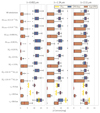 |
Fig. 9 Wavelength-dependent distribution of contrast values CPD: Star and Gap: CPD shown in Tables C.2 to C.4 using boxplots. Each median is highlighted by a red line, the middle 50% of data are represented by a box, and the maximum whisker length equals Δw = 1.5IQR. The labels to the left characterize the data used in generating the corresponding boxplots to the right of the label. The label “All Simulations” in the first row refers to wavelength-dependent but otherwise unrestricted data. In any other case the label refers to a shared parameter value. The wavelength is shown above its corresponding column. The 5σ detection limits Dlim are shown as vertical yellow lines, with arrows indicating the direction of detectable signals. Outliers are shown as black diamonds. For details, see Sect. 3.6. |
 |
Fig. 10 Distribution of contrast value changes of CPD: Star and Gap: CPD with respect to the change in a single model parameter using boxplots. Each median is highlighted by a red line, the middle 50% of data are represented by a box, and the maximum whisker length equals Δw = 1.5 IQR. The labels to the left characterize the data used in generating the corresponding boxplots to the right of the label. A label refers to a parameter that has been increased to its next simulated value. Outliers are shown as black diamonds. For details, see Sect. 3.7. |
3.7 Parameter impact and characterization
Thus far, we have presented an analysis of the potential for detecting embedded planets in the VIS/NIR with a focus on SPHERE. However, the gathered data can also be examined regarding the best approaches for characterizing these planets and their surrounding CPDs. As it turns out, these purposes do not benefit from the same observational strategies. To characterize single basic properties, it is crucial to understand the impact they have on observations, in particular, the sensitivity with which measured contrast values react to a change of a single parameter is important.
To better assess the impact of a parameter change on observations of different models and disentangle the information presented thus far, Fig. 10 illustrates the effect of all varied parameters separately. In particular, we compute the difference of contrast values of two simulations whose underlying parameters differ only in the value of a single parameter and illustrate the distribution of contrast difference values with boxplots. To not restrict this analysis to a specific set of wavelength-dependent inner working angles, we consider all planetary and CPD signals, even if they are labeled Hidden, which allows for a more general analysis.
Generally, an increase in any parameter value may lead to an improved or a worsened contrast. In this context, an improved contrast refers to a contrast change that is beneficial for a detection, for instance a reduced contrast CPD: Star or an increased contrast Gap: CPD. The presented results allow us to identify some clear trends that can be found for the majority of simulations. In order to identify these trends, we mainly focus on the sign of the change in contrast values, particularly of the median, and on the distribution of the middle 50% of data. We also note that even if the median is at about zero, there may still be a difference between the left and right sides of a distribution of data points, in that the data may be left-skewed or right-skewed. In the framework of detectability and characterizability, this translates to an advantageously skewed or disadvantageously skewed distribution of data points, depending on the type of contrast and direction of skewness. This means that an advantageously skewed distribution of data points is either a left-skewed CPD: Star distribution or a right-skewed Gap: CPD distribution. A broad overview of the trends that can be found in Fig. 10 is concisely summarized in Table 4. Additionally, to highlight and discuss some of these findings, we focus only on the key results.
In the following we present an analysis of all studied varied parameters and how their changes affect measurements.
3.7.1 Wavelength dependence
In this parameter study, the observing wavelength λ is a unique parameter in the sense that it is the only parameter that is in the control of the observer. Therefore, this section presents some general trends that can be found for λ and we will have a dedicated in-depth discussion of the best choice for λ for every other parameter separately.
Overall, we find that increasing the observing wavelength λ has the strongest beneficial effect on the contrast CPD: Star, as can be seen in Fig. 10. Moreover, this effect is consistent, meaning that all data points within the IQR are shifted toward a single side. This can be explained by the strong change in optical depth between the observer and the planet. In particular, at λ = 2.11 µm the extinction cross-section, and thus the optical depth, is roughly 3 or 9 times smaller than that at λ = 1.24 µm or at λ = 652 nm, respectively. It is also important to note that the temperature of dust in the CPD has a natural upper limit given by the sublimation temperature. Using Wien’s displacement law as a rough approximation, an upper temperature of ≈1500 K yields a wavelength of λ ≳ 3.4 µm at the peak of spectral flux per unit frequency. As a consequence, the optical depth decreases and the spectral flux of the CPD increases toward larger values of λ. Despite its higher temperature, the planet also increases its spectral flux and benefits from the decreased optical depth.
To further elaborate on these finding, Figs. C.1 and C.2 give a more in-depth view into the impact of a single parameter on the contrast values, which is achieved by also sorting the data into groups of shared parameter values. Similarly to Fig. 9, the shared parameter value is displayed to the left. Here, the increased parameter is shown above its corresponding column. The results for the group of constant rp value in the left column (↑ λ) of Fig. C.1 is particularly interesting. Here we find that the benefit of an increasing wavelength seems to rise rather strongly with rp, particularly in the case of CPD: Star. However, an increase in λ for rp = 5 au simulations is leaving Gap: CPD almost unchanged. At rp = 10 au we find a disadvantageously skewed distribution for Gap: CPD, meaning that the contrast tends to worsen for increasing λ, before drastically improving toward rp = 50 au. Moreover, for rp = 50 au the beneficial effect is becoming very consistent. The fact that this effect is not strictly positive for increasing values of rp may be explained by considering the temperature of the star and its spectral flux, which reaches its highest value at λ = 1.24 µm and dominates the detected flux in the azimuthal gap region (see Sect. 3.3). A negative impact on rp = 10 au simulations suggests that despite the discussed benefits of an increased wavelength, the contrast Gap: CPD may still decrease due to an elevated gap flux level induced by a change in spectral stellar flux.
Overall we conclude that a detection of a planet at larger radii is more likely to benefit from a longer observational wavelength. At shorter distances rp, though, it is rather unlikely to make any detection for different reasons. On the one hand, at shorter wavelengths the optical depth leads to an overall low-contrast CPD: Star that we find to be deep inside the undetectable range. On the other hand, at longer wavelengths we find that the gap region becomes increasingly contaminated, as discussed in Sect. 3.6, diminishing Gap: CPD values to the level of noise. Nonetheless, in this case the CPD: Star values come close to the detectable range. Finally, when comparing the impact of an increase in λ for simulations with shared values of λ, we identify a diminishing return for higher wavelengths. Overall, the explored wavelength dependence suggests that observations at λ = 2.11 µm carry the greatest potential for future detections. A study of the best suited wavelength choice for characterizing basic planetary and CPD properties is presented in each of the following sections for every parameter separately.
3.7.2 rp-dependence
Among all investigated parameters, the radial position of the planet (rp) is the only parameter that when varied usually improves one contrast while worsening the other (see Fig. 10). While an increase in rp improves Gap: CPD strongly and consistently, its effect on CPD: Star varies strongly depending on the underlying model parameters. This can be clearly seen in the middle column (↑ rp) of Fig. C.1. We find that its increase affects rp = 5 au and rp = 10 au simulations in a noticeably different way; specifically, it adversely affects the former and benefits the latter. The difference of median values from the displayed CPD: Star and Gap: CPD distributions, which can be viewed as a measure for the overall impact on the observability of the models, shows a striking increase for increasing rp values. The same is true when increasing the observing wavelength λ, as can be seen in the bottom three rows of Fig. C.1. In particular the median of the CPD: Star simulations shifts from a clearly positive value at λ = 652 nm to a negative value at λ = 2.11 µm, yet again highlighting the combined benefit of models with high rp value observed at longer wavelengths. This trend can also be observed for the shared parameter Mp. Increasing the planetary mass Mp shifts the median of the CPD: Star distribution from positive values toward roughly zero, while clearly benefiting Gap: CPD by shifting it consistently toward higher positive values. Therefore, we find that rp has the most diverse effect on all simulations. This behavior can be explained by two effects. First, rp strongly affects the stellar flux level at the position of the gap and, second, it also strongly impacts the optical depth between the observer and the planet. Therefore, an increase in rp on the one hand decreases the stellar flux level; on the other hand, it exposes the planetary and CPD signal. Our results suggest that both effects compete at a similar level and either one can dominate. For instance, low Mp simulations suffer from a high optical depth, even at higher values of rp, and as a consequence, these planets still appear very dim, which in turn leads to an overall decrease in flux at the position of the planet and an increase in CPD: Star. The higher the Mp, the more planetary and CPD flux is revealed, and the gap further deepens, which leads to a better CPD: Star value change. The same effect as described for fixed increasing Mp values holds for increasing λ values as well, but it is even stronger.
Finally, the parameter rp is unique in that its determination on the basis of directly imaged can be estimated by simply measuring the position of the peak in flux. In that regard, its determination can be best achieved at a wavelength that shows the strongest signal, which we find to be λ = 2.11 µm.
3.7.3 Mp-dependence
For the majority of simulations, higher masses Mp result in better contrast values (see Fig. 10). In particular, the Gap: CPD distribution is strongly advantageously skewed, meaning, more models benefit strongly from an increase in Mp than weakly. Moreover, the right column (↑ Mp) of Fig. C.1 shows interesting dependences on rp and λ. We find that an increase in Mp is particularly beneficial for far-out planets regarding both CPD: Star and Gap: CPD. Here the IQR of CPD: Star is especially noticeable, which is the narrowest for rp = 10 au simulations, where in addition the median is close to but smaller than zero. This is interesting since an increase in Mp causes various effects. First, the optical depth between planet and observer is decreased. Second, the accretion luminosity is increased. Third, the inner radius of the CPD is widened, which changes the density and thermal structure of the CPD as a whole. Fourth, the optical depth in radial direction within the gap is decreased due to the its increased depth, which reduces the scattering probability of stellar photons. The small width of the distribution suggests that these effects are competing with each other and the overall result in similar outcomes when increasing Mp. This is contrary to the scenarios of planets that are located either farther in or farther out. The latter especially tend to greatly benefit from an increase in Mp. In order to identify one of the modeled planets it is crucial to observe at a wavelength where the observed contrast levels are the most diverse. Judging from the IQRs of both contrasts for different wavelengths we find that it is the widest for short wavelengths (i.e., at λ = 652nm). Combining these results with results from Sect. 3.6, we find that the chances for detectability and the capability of characterizing the planetary mass directly counteract each other in the sense that a single wavelength observation can improve one only by diminishing the other.
3.7.4  -dependence
An increase in the accretion rate onto the planet  leads to a proportional increase in Lacc, which leads to an advantageously skewed distribution of contrast changes according to Fig. 10. Compared to the other parameters, these differences are small as the median is at zero and the IQR is rather narrow. On the one hand, the fact that all of the medians of the boxes match their corresponding box edges, which are placed with contrast differences of zero, shows that a large part of models would not benefit from an increase in
  . On the other hand, the large number of outliers also shows that a significant portion of simulations are actually affected far beyond the level of noise. Moreover, we find that an increase often results in a negative impact on both contrast values as well. The left column
  in Fig. C.2 also shows that negatively impacted outliers for the two contrast values are caused under different circumstances. In particular, negatively impacted outliers of CPD: Star, which distinguish themselves due to high positive values, are typically based on simulations with higher planetary masses Mp, while outliers of Gap: CPD, which have high negative values, usually originate in simulations with low values of Mp. The most positively impacted outliers, though, are caused for both contrasts in simulations with higher planetary mass. Similarly, we find that the most negatively impacted outliers of CPD: Star and Gap: CPD are caused for close-in and far-out planets, respectively, while most positively impacted outliers come from far-out rp = 50 au simulations for both contrast distributions. Moreover, we find that the simulated observations react most sensitively to changes of
  when observed at the shortest simulated wavelength λ = 652 nm. At longer wavelengths, the impact of
  is much weaker, although it has the potential for the highest negative outliers regarding CPD: Star.
As mentioned before, the primary effect of increasing  is an increase in the accretion luminosity Lacc, which in turn results, first, in an extended inner radius rin;p of the CPD that is changing its density and thermal structure and, second, in higher spectral planetary flux. Since both effects are confined to the planet and its vicinity and since this region is deeply embedded in the CSD, the impact of a change in
  at any observational wavelength best shows when the region is exposed the most, which means that when the optical depth between the observer and the planet is the lowest. This explains the increase in the IQR of simulations with higher values of Mp or rp. Since the increase in
  strictly increases the planetary flux, a negative impact is mostly the result of a reduction of the observed spectral CPD flux. The most negatively impacted outliers of CPD: Star, for instance, come from simulations with high values for Mp and MCPD and with low values of rp. This coincides exactly with the dependences found for increasing rin;p values in Sect. 3.1. Thus, more extended CPDs are more likely to result in worse CPD: Star values when being further extended due to an increase in
  . For Gap: CPD, however, the situation is more complicated. Due to the locality of induced changes, one might expect that the measured contrast values CPD: Star and Gap: CPD behave in exactly the same way except for their sign (i.e., that the distributions are mirrored). However, this is not the case, as can already be seen in Fig. 10. Figure C.2 shows mirrored distributions only for the rp ≥ 10 au and for Mp = 0.25 MJ simulations. What these simulations have in common is either that they harbor relatively far-out planets or generally planets with low Lacc. On the other hand, it is those simulations with close-in planets and high accretion rates Lacc that typically cause the asymmetry between the two distributions. The reason is that for these simulations the aforementioned argument of locality does not apply, meaning that a change in
  affects the whole contaminated gap region, which is why these simulations are labeled Contaminated in Tables C.2 to C.4. The effect is only present in the rp = 5 au simulations and enhanced by higher values of Lacc particularly at longer observation wavelengths, which is in agreement with our results regarding
  and generally simulations that do not satisfy the condition in Eq. (17). Overall, we conclude that observations aimed at detecting mass accretion rates ought to take into account primarily short observational wavelengths given their higher level of sensitivity regarding
  .
.
3.7.5 MCPD-dependence
Of all the investigated parameters, the mass of the CPD (MCPD) has the smallest overall impact on the two contrast values. While both contrast distributions in Fig. 10 are advantageously skewed, a large portion of their data points fall into a very narrow IQR. Moreover, outliers are even more abundant in these distributions than they are in those corresponding to an increase in the planetary mass accretion rate  . In the middle column (↑ MCPD) of Fig. C.2 we find that the widest IQRs can be found for rp = 50 au and λ = 2.11 µm simulations. The overall narrowness of most IQRs, though, can be explained by considering the effect that a change in MCPD induces. Already at MCPD = 0.1 × 10⁻³ MJ the CPD is optically thick at all investigated wavelengths; therefore, increasing it mostly causes a strengthening of the back-warming effect (see Sect. 3.1). As a consequence, the inner radius rin;p increases and the thermal and density structure of the CPD changes. Within the investigated parameter space MCPD has the greatest impact on rin;p, as can be seen in Table C.1. Despite its overall weak impact, we generally find that this redistribution of dust grains induced by an increase in dust mass in the CPD is beneficial for a detection; this means that the back-warming effect is acting in favor of this goal, in particular at λ = 2.11 µm, where the impact is the greatest. Similarly to
  , we also find that some distributions of Gap: CPD and CPD: Star are linked, in that they are symmetric and only differ in the sign of change. Here we observe this type of symmetry, yet again, for far-out planets at rp ≥ 10 au, as well as a relatively strong symmetry for wavelengths λ ≤ 1.24 µm. At rp = 5 au, however, this effect cannot be found, which is most likely due to contaminated contrast values, analogously to the case of
  . Contrary to the results for
  , we conclude that the highest sensitivity for an observationally based measurement of MCPD can be achieved at longer wavelengths, particularly at λ = 2.11 µm. These results are expected since the temperature of the CPD typically reaches values far below the planetary temperature, and thus has its emission maximum shifted toward longer wavelengths.
3.7.6 MCSD-dependence
The CSD mass MCSD plays a crucial role in the detectability of embedded planets, which can be seen in the corresponding contrast distributions in Fig. 10. Judging from the medians, we find that the majority of simulations strongly benefit from a reduction in MCSD, particularly the Gap: CPD distribution, which additionally shows a very consistent beneficial result. In the right column (↑ MCSD) of Fig. C.2 we find some clear trends regarding the interplay of MCSD and rp. Here, the total range of data points of both contrast values strictly increases with rp and the medians are shifted increasingly toward an unfavorable direction. At rp = 50 au both contrast distributions are very consistent, meaning that all data points within each IQR share the same sign. In contrast, at rp = 5 au the CPD: Star distribution is strongly advantageously skewed and the IQR extends deeply into the beneficial range. Therefore, there are instances where an increase in MCSD actually is beneficial for the detectability of an embedded planet. However, this is mostly restricted to close- in planets, which are unfortunately difficult to detect. Regarding the wavelength dependence we find that the IQR of CPD: Star distributions is significantly wider at λ = 652 nm compared to the longer wavelengths. At this wavelength, we also find the largest fraction of beneficial contrast differences. According to the different results from Fig. C.2 we find that the fraction of models that benefit from an increase in MCSD mostly consist of simulated planets at rp = 5 au when observed at λ = 652 nm. Moreover, these planets are rather low in mass and particularly Mp = 0.5 MJ planets seem to cause this effect. Furthermore, since the CPD: Star distributions for the parameters MCPD and Mp only show weak differences among shared values, we conclude that this is for the most part an optical depth effect. That this occurs more often for farther-in planets suggests that the effect is most likely caused by scattered stellar flux, and is therefore less dependent on the optical depth between the observer and the planet than on the optical depth as observed from photons that are emitted from the star and scatter off dust grains located inside the gap. This hypothesis is further supported by the fact that at rp = 5 au the Gap: CPD distribution is extremely narrow and even centered around zero. When trying to deduce the mass of the CSD solely using VIS/NIR data, these results suggest that different values of MCSD can be best distinguished when observing at λ = 652 nm.
3.8 Caveats
This study presents and applies a method of testing the abilities of SPHERE to detect and characterize embedded planets. In this section we assess potential caveats regarding the method and underlying assumptions. In this context we discuss the robustness of our method, the impact of the chemical composition of the dust and of the inclination angle, and finally the existence and potential structure of the CPD. Further elaborating on these topics, for instance in the framework of a broad parameter study, would certainly deepen our understanding of the capabilities of SPHERE. Based on the results of this study, though, we can only attempt to estimate the relevance these topics.
The method we used to quantify the strength of the planetary and CPD signal involves the determination of three different regions: the azimuthal CPD region, the gap region, and the transition region. The robustness of this method thus depends on the capability of properly identifying them. This process, however, may be performed inaccurately either due to the misidentification of the position of the potential planet or due to an incorrect estimation of the radius  from Eq. (16). The consequence of such an error certainly depends on its severity; however, small errors can be expected to only result in slight changes of the outcome. If, for instance, the azimuthal CPD region is slightly shifted but still covers the brightest local region at the position of the planet, the subsequently determined signal strength of the planet and CPD will be reduced. However, due to the averaging that is involved in the calculation of the radial CPD region only a fraction of the flux is lost, which stems from the rim of the azimuthal CPD region. Similarly, if the estimation of the azimuthal gap region is slightly off, the azimuthal averaging of the gap profile suppresses potentially considered contaminated flux that once more stems from the rim of the azimuthal gap region. Thus, it can be expected that both errors only slightly lower the determined planetary and CPD signal at any observed wavelength.
Next, we discuss different assumptions that were made in the course of this study. The chemical composition of dust in general plays a crucial role for the observed properties of a PPD. Even though silicates and carbonaceous material make up a significant portion of dust in the interstellar medium and consequently in CSDs (e.g., Draine 2003; Lommen et al. 2010), it can be expected that these disks contain various other materials as well (e.g., in the form of water ice). To reduce the complexity of the modeled systems we focused on these key components, even though an extended study with a particular focus on the dust composition, size, and shape would certainly add to our findings.
Furthermore, we assumed the disk to be observed face-on (i.e., an inclination angle of i = 0°). This angle has an impact on the optical depth between the observer and the embedded planet, and thus influences the attenuation of light originating from the planet and its CPD before its detection. As a function of the orbital phase angle of the planet the determined excess signal strength of the planet and CPD thus varies. Overall, it can be expected that an inclined CSD would often lead to an increase in the optical depth, and as a result would lower the possibility of unveiling planets, making their direct detections in more inclined disks more challenging.
Moreover, we made a particular choice for the model of a CPD. However, to date, none of the modern instruments is capable of providing a high-resolution image of any such disk. To provide the most reliable results, this study assumes models of a CPD that are constructed based on results of state-of-the-art hydrodynamics simulations. Since the thermal and density structure of the CPD determines its detectability, a different model or the complete absence of the CPD may very well change the determined signal strength. Consequently, conducting a similar study but using a model of a circumplanetary envelope or even assuming the lack of any circumplanetary material instead would certainly be insightful. However, since the presence of CPDs seems to be a very likely scenario for the range of considered planetary masses, it can be expected that the results of this study apply to a wide range of PPDs harboring young accreting planets.
4 Summary and conclusions
We present a study on the detectability and characterizability of embedded low-mass giant planets in gaps of CSDs of typical T Tauri stars in the VIS/NIR wavelength range. To this end, we performed fully self-consistent MCRT simulations using the code Mol3D (Ober et al. 2015) for 72 models and three different observing wavelengths (652 nm, 1.24 µm, and 2.11 µm) each. Our model is composed of a central star that is surrounded by a CSD in which a planet is harbored that carves a gap into the CSD as it accretes material. The models make use of empirically determined gap profiles (Kanagawa et al. 2016, 2017; Gyeol Yun et al. 2019) and the embedded planets themselves are surrounded by optically thick CPDs and emit accretion luminosity, thus heating up the corresponding environment. The parameter domain that is covered by the models is described in Table 1 and contains, in addition to the wavelength λ, five other parameters: the planetary mass Mp, the planet’s distance to the star rp, its mass accretion rate  , the CPD mass MCPD, and the CSD mass MCSD. In order to properly treat the extremely high optical depths encountered in CPDs we made use of a method for optically thick dusty media as introduced by Krieger & Wolf (2020). Furthermore, a method to access the impact of a planet and its CPD was introduced that distinguishes between three azimuthally divided regions in the CSD: the azimuthal gap region, the azimuthal CPD region, and the transition region that separates these two regions. This method utilizes a procedure to convert a Cartesian detector grid to a polar detector grid, for which the python package CartToPolarDetector was specifically written, and which is described in Appendix B. The measured and quantified impact of a planet and its CPD on observations in the VIS/NIR is summarized in Tables C.2 to C.4, and subsequent analyses of these data were presented throughout this paper. The results are summarized in the following:
We apply a detection criterion (see Sect. 3.6) based solely on the contrast between the stellar and the planetary and CPD region (CPD: Star) which is λ- and rp-dependent, and find that the majority of simulations in the investigated part of the parameter space would result in a non-detection of the planetary and CPD signal when using SPHERE. However, there are simulations that satisfy our condition for detectability even within the studied parameter domain. In particular, we find that all investigated simulations at rp ≤ 10 au are not detectable, and only far-out planets have a chance to be detected;
-
According to our results, a non-detection far-out at rp = 50 au can still be used to restrict the underlying properties of a potential embedded planet which depend on the wavelength at which the observation was performed. Considering the trends found in Fig. 10 and described in Table 4, these are our findings.
First, using ZIMPOL at λ = 652 nm, a non-detection implies
- (i)
Mp < 1 MJ or
 for MCSD = 0.01 M⊙, and
 - (ii)
(
 ) or Mp < 0.5 MJ for MCSD = 0.001 M⊙.
Second, using IRDIS at λ = 1.24 µm, a non-detection implies (i) Mp < 0.5 MJ or
 for MCSD = 0.01 M⊙, and
 - (iii)
Mp < 0.25 MJ or
 for MCSD = 0.001 M⊙.
Third, using IRDIS at λ = 2.11 µm, a non-detection implies Mp < 0.25 MJ or
 for both MCSD = 0.01 M⊙ and MCSD = 0.001 M⊙. Overall, our results within the VIS/NIR wavelength range suggest that observations at λ = 2.11 µm provide the greatest potential for future detections, which in the case of SPHERE is possible using IRDIS.
- (i)
The characterization of the planets and their CPDs has been studied with regard to the observing wavelength and five different other parameters. We find that characterizing and detecting low-mass giant planets in gaps in the VIS/NIR wavelength range often benefit from the contribution of various observing wavelengths (see Sect. 3.7). In the following we present a list of our key findings regarding the relevance and impact of each of those studied parameters on the characterizability of directly imaged planets:
- (a)
The distance between the star and the planet rp is decisive for the detectability. In general, its increase can both improve and worsen the contrast CPD: Star. However, far-out planets strongly benefit from high values of rp due to the effect on the optical depth between the planet and the observer, which decreases as rp increases and thus exposes the planetary and CPD signal. Since the position of a directly imaged planet can be inferred straightforwardly from the position on the image, we find that its determination has the greatest potential at longer wavelengths when the chances for a detection are the highest (i.e., at λ = 2.11 µm);
- (b)
The planetary mass Mp is highly responsible for the observed planetary and CPD signal. Judging from the high sensitivity with which the observed planetary signal reacts to a change in Mp within the studied parameter domain, we find that observations at λ = 652 nm are best suited for its characterization;
- (c)
The mass accretion rate
 onto the planet has a comparably weak impact on the observed contrast values. We find a correlation between CPD: Star and the inner radius of the CPD rin;p when varying
  . In particular, for increasing
  values the contrast CPD: Star often worsens as rin; p further increases. Overall, our results suggest that λ = 652 nm is the best suited observing wavelength for distinguishing between different values of
  ;
; - (d)
Overall, the CPD mass MCPD has the smallest impact on the measured contrast values, making it the most difficult to determine in the investigated parameter domain. We find that its increase shows the trend to improving the observed signal of the planet and CPD. Moreover, its characterizability benefits the most from longer observing wavelengths (i.e., λ = 2.11 µm) since an increase (decrease) of MCPD mainly induces a strengthening (weakening) of the back-warming effect (see Sect. 3.1), which primarily affects the thermal radiation of the CPD;
- (e)
The CSD mass MCSD plays a crucial role in the detectability of an embedded planet. Most systems benefit from a reduction of MCSD; however, we also identified a potentially beneficial effect for CPD: Star from its increase for far-in planets and in particular planets of mass Mp = 0.5 MJ, which we attribute to an optical depth effect (for details see Sect. 3.7.6). Within the VIS/NIR wavelength range we find that the best suited observing wavelength for distinguishing between different values of MCSD is λ = 652 nm.
- (a)
An analysis of planetary signals that are blocked by a coronagraphic mask clearly suggests that the current capabilities of SPHERE regarding the detection of embedded planets are not limited by the use of a coronagraph (see Sect. 3.6). In particular, we find that the majority of simulated planets whose signal is blocked by the coronagraphic mask, which in our case are planets at rp = 5 au that are observed with ZIMPOL at λ = 652 nm, result in very low CPD: Star values, which are well inside the undetectable range. In addition, we find that the majority of these systems generate contrast values between the gap and the planetary and CPD region of Gap: CPD < 1 mag. Consequently, this clearly suggest that decreasing the IWA would not result in any more detections of planets that are within the studied parameter domain when using SPHERE/ZIMPOL;
Our applied method for quantifying the planetary and CPD signal includes the definition of a contamination-free azimuthal gap region, which is defined via the wavelength-dependent radius
 and the distance between the star and the planet rp. In Sect. 3.6 we find that the contrast Gap: CPD is strikingly reduced for all contaminated systems, which is likely a consequence of an elevated flux level of the contaminated gap. The contrast reaches in all simulated cases values of only Gap: CPD < 0.2 mag. This shows, first of all, that our definition of the azimuthal gap region via
  in Eq. (16) together with the condition for a contamination-free gap in Eq. (17) is reliably categorizing systems with low contrast values and, second, that the detection of embedded planets that do not satisfy the condition in Eq. (17) is indeed extremely challenging;
We find that the inner radius of the CPD rin;p is strongly affected by the back-warming effect described in Sect. 3.1. As a consequence, we find that when keeping the remaining parameters constant the inner radius of the CPD (rin; p) increases if rp decreases, Mp increases, Mp increases, or MCPD increases. Its dependence on MCSD is shown to be comparably weak. A change in rin; p leads to a change in the thermal and density structure of the CPD, which consequently affects its spectral energy distribution. This is relevant since we find that the thermal radiation of the CPD may strongly contribute to the measured flux at the position of the planet (see Sect. 3.3), in particular the self-scattered part of its thermal radiation since the direct part is highly attenuated by the optical depth between the planet and the observer.
Finally, it is possible to evaluate the fact that to this day only the planets PDS 70 b and PDS 70 c have been confirmed by direct imaging. Even though these two giant planets are outside the investigated parameter domain, the trends we find are very much in line with the observations, since we find great benefits for the contrast for high values of rp and Mp. We find this to be particularly the case for SPHERE/IRDIS observations, which were also part of the multiwavelength analysis that was performed to confirm the presence of these planets. It is interesting, though, that our parameter study reveals the possibility for detecting significantly lower planets with a mass of Mp = 1 MJ using SPHERE. However, such a detection seems to be only feasible in the case of far-out planets with high mass accretion rates and especially low CSD masses leading to a lower optical depth between the observer and the planet.
Nonetheless, to reliably deduce the presence of a low-mass giant planet embedded in a gap of a CSD it is crucial to perform multiwavelength observations. This is not only increasing the chances for detecting such a planet but is at the same time beneficial for its characterization, since we have seen that different wavelengths, even within the VIS/NIR wavelength range, possess different potentials for characterizing the various basic properties of both the planet and its CPD. Therefore, to assess the full potential for detecting and characterizing embedded planets, it would be important to conduct another study focusing primarily on the millimeter and submillimeter wavelength range. This would allow us to evaluate the potential for detecting and confirming additional planets in the future either by using state-of-the-art or future instrumentation. In addition, it may provide new insights that help guide the planning and design of future observatories in the quest for observing embedded accreting planets while they form.
Acknowledgements
We thank all the members of the Astrophysics Department Kiel for helpful discussions and remarks. We acknowledge the support of the DFG priority program SPP 1992 “Exploring the Diversity of Extrasolar Planets (WO 857/17-1)”. This research has made use of seaborn (Waskom 2021), a library for making statistical graphics in python.
Appendix A Back-warming in 1D
To explain the back-warming effect, we use a one-dimensional mono-chromatic model that is composed of a isotropically radiating light source in a vacuum that illuminates a one-dimensional connected density distribution (slab) of total optical thickness τb = 2b. In this section we show how the temperature distribution inside the slab changes as its density changes. In particular, we show that the temperature at the inner edge of the slab (i.e., the illuminated edge) increases and the temperature of the outer edge decreases when the density of the slab is increased. Since the effect is independent of the albedo A of the medium, we chose A = 1.
The derivation of the resulting temperature distribution presented in this section is fully based on the eigenstate-based description of this problem introduced by Krieger & Wolf (2021) (hereafter KW21).
The initial distribution of photons ν0(x) is described by
 (A.1)
(A.1)
where x ∈ [−b, b] is the optical depth coordinate and δ(x) the delta distribution. A portion of the emitted photons enter the slab and are absorbed and reemitted, potentially multiple times, before all photons eventually (i.e., in the limit of n → ∞ interactions) leave the slab through either of its edges. The distribution of photons that interacted n times is described by
 (A.2)
(A.2)
where ak and bk are expansion coefficients of ν0(x); λk and are the eigenvalues of eigenstates cos(σkx) and sin(σkx), respectively; and A is the albedo, which in our case is 1. Applying Eqs. (A.13) to (A.16) from KW21 gives
 (A.3)
(A.3)
The temperature at any point of the slab is determined by the ambient radiation field at that point. The quantity νtot(x) is a measure of the radiation field and is given by
 (A.4)
(A.4)
Using the previous equations and applying Eqs. A.6 to A.8, A.39, and A.43 from KW21, we arrive at
 (A.5)
(A.5)
Therefore, the radiation field reaches its maximum at the inner edge, where  , and its minimum at the outer edge, where
  . Here, we use the optical depth coordinate x rather than a spatial coordinate. Thus, an increase in total optical depth is equivalent to an increase in density of the medium. According to Eq. A.5, the radiation field consequently increases with increasing optical depth b. In other words, if a photon exits a slab at its outer edge, it will no longer increase the temperature of the slab, unless more optical depth is added the outer edge, which has the potential to interact with the photon and warm up the slab from the back. This effect is called back-warming.
Interestingly, even though the slab warms up at the inner edge and cools down at the outer edge, when increasing the density the average temperature of the slab in this one-dimensional setup stays constant. This is the case since the average radiation field, according to Eq. A.5, is constant and in particular independent of the optical depth τb. Additionally, this can be shown by calculating the mean traversed path length of photons traveling through the slab, which is given by
 (A.6)
(A.6)
where l(x) is the mean optical depth traversed by a neutral photon package (i.e., weight equals 1), originating from position x within one step of interaction. The quantity l(x) contains contributions from photons that leave the slab through its inner edge, from photons that are absorbed inside the slab, and from photons that leave the slab through the outer edge. It is thus given by
 (A.7)
(A.7)
Performing the integration in Eq. A.6 yields
 (A.8)
(A.8)
The mean length traversed by a photon that enters the slab is therefore exactly given by the optical depth of the slab. In this one-dimensional case, the mean deposited energy per optical depth unit for photons that enter the slab thus equals 〈l〉/τb = 1 and does not depend on τb.
Appendix B Converting Cartesian to polar detector
In this section we describe the basic principle of the python package CartToPolarDetector which is used to convert a Cartesian detector into its polar representation. The original Cartesian detector is described by Nx and Ny pixels of equal width in x-direction and y-direction, respectively. Each of these pixels has an assigned flux density value measured in Jy. Properties of the desired polar grid can be defined by the user. In particular, the grid is defined by the position of its center with regard to the original grid (shift), its radial extent, the number of cells in ϕ-direction Nϕ, and the number of cells in r-direction Nr. By default, the shift is deactivated, meaning the two grid centers coincide, and the radial extent is chosen, such that the whole Cartesian detector is embedded in the polar detector. Nr and Nϕ can take any integer number greater than zero; however, Nϕ must be divisible by four.
During its execution, the code loops over all Cartesian pixels and classifies each pixel’s respective position relative to the polar grid center with terms such as left, right, top, bottom, middle, or combinations of them. Then, the ϕ-range is determined in which polar pixels may intersect with the Cartesian pixel. Since any determined intersection area of two pixels does not change when the detectors rotate, the detectors are rotated by an integer multiple of π/2 such that the new Cartesian pixel position is either in the top or in the top right position. An exception to this is made only in the case that the position is initially classified as middle, which means that the polar center is inside the pixel, but not in any of the pixel’s edges or corners, in which case no rotation is performed. Such a pixel is unique and is treated separately. After the intersection area calculation step, the pixels are rotated back and the corresponding contributions of Cartesian pixels to polar pixels are added to the polar grid. The assigned value that is added to a polar pixel is a product of the value assigned to the Cartesian pixel and the ratio of the corresponding intersection area to the total area of the Cartesian pixel. In a last step, after all Cartesian pixels have been looped over and the polar grid has been calculated, it is stored. Additionally, all input parameters as well as a list of pixel border values for ϕ and r are stored, where ϕ and r are measured in radians and in original Cartesian pixels, respectively.
 |
Fig. B.1 Integrated intersection area (orange). It is the intersection area of a Cartesian pixel (black) with a segment of a circle (blue) and it is assigned to a polar pixel (hatched region) that is defined by an inner radius rinner, an outer radius router, a left border ϕl and a right border ϕr. The overlayed polar grid is shown in gray and the two radial and angular borders of a selected polar pixel are highlighted in dark gray. |
The calculation of the intersection area is the most complicated step in terms of the number of possible ways an arbitrarily shaped polar pixel can intersect a Cartesian pixel. However, in-stead of showing the exact intersection formula for all cases, we briefly summarize the general approach by which they were obtained. However, to remove some of the complexity of this step, we divide it into two parts. In the first part we determine an integrated intersection area. Figure B.1 illustrates the concept of the integrated intersection area. A polar pixel is defined by an inner and an outer radius, as well as two ϕ borders. Since we are dealing with pixels that, after a potential rotation, are located in the top region or top right region, we can define one ϕ border as the left and the other ϕ border as the right border, where the right border ϕr is pointing more toward the direction of the positive x-axis than the left border ϕl. In the upper half of this plot a segment of a circle (blue) can be defined by the outer pixel radius and covering the range from ϕ = −π/2 to the right border ϕr, as can be seen in the plot, where ϕ = 0 corresponds to the direction of the positive y-axis. The integrated intersection area (orange) is then the intersection area of this segment of the circle with the Cartesian pixel (black). It is called the integrated intersection area as it contains the desired individual intersection area (hatched), but may also contain intersection areas that belong to other polar pixels.
In the second part of this calculation, the individual contributions can easily be obtained after determining the integrated intersection areas of all relevant polar pixels. Let Si,j the integrated intersection area of a polar pixel (i, j), where i and j are non-negative integers with i < Nϕ and j < Nr, and let Ii,j the individual intersection area of that same pixel, then we find for all pixels in the upper half the relation
 (B.1)
(B.1)
where mod denotes modulo operation. Due to the previously performed rotation, polar pixels in the lower half do not intersect with the Cartesian pixel.
Appendix C Results
Compilation of results for all simulated models at λ = 652 nm. The first five columns give the set of underlying parameter values. Contrast values (in mag) are obtained based on either of two types of features (Gap or Kink). Hidden planets are flagged with a cross and refer to planets whose inferred position of the planetary and CPD signal is hidden inside the IWA of the corresponding coronagraph, which can be found in Tab. 2. Contaminated planetary and CPD signals are flagged with a cross in the “Cont” column and correspond to simulations that do not satisfy the condition stated in Eq. (17). The last five columns refer to contrast values either with respect to the stellar (Star) flux or to the flux of the gap region (Gap), where the following abbreviations were used: Coronagraph (C), ring (R), planet and CPD (CPD). For details, see Sect. 3.5.
Compilation of results for all simulated models at λ = 1.24µm. The first five columns list the set of underlying parameter values. Contrast values (in mag) are obtained based on either of the two types of features (Gap or Kink). Hidden planets are flagged with a cross and refer to planets whose inferred position of the planetary and CPD signal is hidden inside the IWA of the corresponding coronagraph, which can be found in Tab. 2. Contaminated planetary and CPD signals are flagged with a cross in the “Cont.” column and correspond to simulations that do not satisfy the condition stated in Eq. (17). The last five columns refer to contrast values either with respect to the stellar (Star) flux or to the flux of the gap region (Gap), where the following abbreviations were used: Coronagraph (C), ring (R), planet and CPD (CPD). For details, see Sect. 3.5.
Compilation of results for all simulated models at λ = 2.11 µm. The first five columns give the set of underlying parameter values. Contrast values (in mag) are obtained based on either of the types of features (Gap or Kink). Hidden planets are flagged with a cross and refer to planets whose inferred position of the planetary and CPD signal is hidden inside the IWA of the corresponding coronagraph, which can be found in Tab. 2. Contaminated planetary and CPD signals are flagged with a cross in the “Cont” column and correspond to simulations that do not satisfy the condition stated in Eq. (17). The last five columns refer to contrast values either with respect to the stellar (Star) flux or to the flux of the gap region (Gap), where the following abbreviations were used: Coronagraph (C), ring (R), planet and CPD (CPD). For details, see Sect. 3.5.
 |
Fig. C.1 Distribution of contrast value changes in CPD : Star and Gap : CPD with respect to the change in a single model parameter using boxplots. Each median is highlighted by a red line, the middle 50% of data are represented by a box, and the maximum whisker length equals ∆w = 1.5 IQR. The labels to the left characterize the data used in generating the corresponding boxplots to the right of the label. A label refers to a shared parameter value. The label above any column refers to a parameter that has been increased to its next simulated value. Outliers are shown as black diamonds. For details, see Sect. 3.7. |
 |
Fig. C.2 Distribution of contrast value changes in CPD : Star and Gap : CPD with respect to the change in a single model parameter using boxplots. Each median is highlighted by a red line, the middle 50% of data are represented by a box, and the maximum whisker length equals ∆w = 1.5 IQR. The labels to the left characterize the data used in generating the corresponding boxplots to the right of the label. A label refers to a shared parameter value. The label above any column refers to a parameter that has been increased to its next simulated value. Outliers are shown as black diamonds. For details, see Sect. 3.7. |
References
- Andrews, S. M., Wilner, D. J., Hughes, A. M., Qi, C., & Dullemond, C. P. 2009, ApJ, 700, 1502 [CrossRef] [Google Scholar]
- Andrews, S. M., Huang, J., Pérez, L. M., et al. 2018, ApJ, 869, L41 [NASA ADS] [CrossRef] [Google Scholar]
- Avenhaus, H., Quanz, S. P., Garufi, A., et al. 2018, ApJ, 863, 44 [NASA ADS] [CrossRef] [Google Scholar]
- Ayliffe, B. A., & Bate, M. R. 2009, MNRAS, 397, 657 [Google Scholar]
- Bae, J., Zhu, Z., Baruteau, C., et al. 2019, ApJ, 884, L41 [NASA ADS] [CrossRef] [Google Scholar]
- Benisty, M., Bae, J., Facchini, S., et al. 2021, ApJ, 916, L2 [NASA ADS] [CrossRef] [Google Scholar]
- Beuzit, J. L., Vigan, A., Mouillet, D., et al. 2019, A&A, 631, A155 [NASA ADS] [CrossRef] [EDP Sciences] [Google Scholar]
- Bjorkman, J. E., & Wood, K. 2001, ApJ, 554, 615 [NASA ADS] [CrossRef] [Google Scholar]
- Bowler, B. P. 2016, PASP, 128, 102001 [Google Scholar]
- Calcino, J., Christiaens, V., Price, D. J., et al. 2020, MNRAS, 498, 639 [CrossRef] [Google Scholar]
- de Boer, J., Salter, G., Benisty, M., et al. 2016, A&A, 595, A114 [NASA ADS] [CrossRef] [EDP Sciences] [Google Scholar]
- Dong, R., & Fung, J. 2017, ApJ, 835, 146 [NASA ADS] [CrossRef] [Google Scholar]
- Dong, R., Fung, J., & Chiang, E. 2016, ApJ, 826, 75 [Google Scholar]
- Draine, B. T. 2003, ARA&A, 41, 241 [NASA ADS] [CrossRef] [Google Scholar]
- Draine, B. T., & Lee, H. M. 1984, ApJ, 285, 89 [NASA ADS] [CrossRef] [Google Scholar]
- Draine, B. T., & Malhotra, S. 1993, ApJ, 414, 632 [Google Scholar]
- Dullemond, C. P., & Penzlin, A. B. T. 2018, A&A, 609, A50 [NASA ADS] [CrossRef] [EDP Sciences] [Google Scholar]
- Flock, M., Ruge, J. P., Dzyurkevich, N., et al. 2015, A&A, 574, A68 [NASA ADS] [CrossRef] [EDP Sciences] [Google Scholar]
- Fouchet, L., Gonzalez, J. F., & Maddison, S. T. 2010, A&A, 518, A16 [NASA ADS] [CrossRef] [EDP Sciences] [Google Scholar]
- Galli, P. A. B., Bertout, C., Teixeira, R., & Ducourant, C. 2015, A&A, 580, A26 [NASA ADS] [CrossRef] [EDP Sciences] [Google Scholar]
- Garufi, A., Quanz, S. P., Schmid, H. M., et al. 2016, A&A, 588, A8 [NASA ADS] [CrossRef] [EDP Sciences] [Google Scholar]
- Garufi, A., Benisty, M., Pinilla, P., et al. 2018, A&A, 620, A94 [NASA ADS] [CrossRef] [EDP Sciences] [Google Scholar]
- Ginski, C., Stolker, T., Pinilla, P., et al. 2016, A&A, 595, A112 [NASA ADS] [CrossRef] [EDP Sciences] [Google Scholar]
- Gonzalez, J. F., Laibe, G., & Maddison, S. T. 2017, MNRAS, 467, 1984 [NASA ADS] [Google Scholar]
- Gräfe, C., Wolf, S., Guilloteau, S., et al. 2013, A&A, 553, A69 [NASA ADS] [CrossRef] [EDP Sciences] [Google Scholar]
- Gyeol Yun, H., Kim, W.-T., Bae, J., & Han, C. 2019, ApJ, 884, 142 [NASA ADS] [CrossRef] [Google Scholar]
- Haffert, S. Y., Bohn, A. J., de Boer, J., et al. 2019, Nat. Astron., 3, 749 [Google Scholar]
- Hartmann, L., Calvet, N., Gullbring, E., & D’Alessio, P. 1998, ApJ, 495, 385 [Google Scholar]
- Isella, A., Benisty, M., Teague, R., et al. 2019, ApJ, 879, L25 [Google Scholar]
- Kanagawa, K. D., Muto, T., Tanaka, H., et al. 2016, PASJ, 68, 43 [NASA ADS] [Google Scholar]
- Kanagawa, K. D., Tanaka, H., Muto, T., & Tanigawa, T. 2017, PASJ, 69, 97 [NASA ADS] [CrossRef] [Google Scholar]
- Keppler, M., Benisty, M., Müller, A., et al. 2018, A&A, 617, A44 [NASA ADS] [CrossRef] [EDP Sciences] [Google Scholar]
- Klahr, H., & Kley, W. 2006, A&A, 445, 747 [NASA ADS] [CrossRef] [EDP Sciences] [Google Scholar]
- Krieger, A., & Wolf, S. 2020, A&A, 635, A148 [NASA ADS] [CrossRef] [EDP Sciences] [Google Scholar]
- Krieger, A., & Wolf, S. 2021, A&A, 645, A143 [NASA ADS] [CrossRef] [EDP Sciences] [Google Scholar]
- Laor, A., & Draine, B. T. 1993, ApJ, 402, 441 [NASA ADS] [CrossRef] [Google Scholar]
- Lommen, D. J. P., van Dishoeck, E. F., Wright, C. M., et al. 2010, A&A, 515, A77 [NASA ADS] [CrossRef] [EDP Sciences] [Google Scholar]
- Lucy, L. B. 1999, A&A, 344, 282 [NASA ADS] [Google Scholar]
- Lynden-Bell, D., & Pringle, J. E. 1974, MNRAS, 168, 603 [Google Scholar]
- Madlener, D., Wolf, S., Dutrey, A., & Guilloteau, S. 2012, A&A, 543, A81 [NASA ADS] [CrossRef] [EDP Sciences] [Google Scholar]
- Marleau, G.-D., Klahr, H., Kuiper, R., & Mordasini, C. 2017, ApJ, 836, 221 [Google Scholar]
- Marleau, G.-D., Mordasini, C., & Kuiper, R. 2019, ApJ, 881, 144 [Google Scholar]
- Mathis, J. S., Rumpl, W., & Nordsieck, K. H. 1977, ApJ, 217, 425 [Google Scholar]
- Mesa, D., Keppler, M., Cantalloube, F., et al. 2019, A&A, 632, A25 [NASA ADS] [CrossRef] [EDP Sciences] [Google Scholar]
- Momose, M., Morita, A., Fukagawa, M., et al. 2015, PASJ, 67, 83 [Google Scholar]
- Mordasini, C., Marleau, G. D., & Mollière, P. 2017, A&A, 608, A72 [NASA ADS] [CrossRef] [EDP Sciences] [Google Scholar]
- Müller, A., Keppler, M., Henning, T., et al. 2018, A&A, 617, L2 [Google Scholar]
- Ober, F., Wolf, S., Uribe, A. L., & Klahr, H. H. 2015, A&A, 579, A105 [NASA ADS] [CrossRef] [EDP Sciences] [Google Scholar]
- Pinte, C., Fouchet, L., Ménard, F., Gonzalez, J. F., & Duchêne, G. 2007, A&A, 469, 963 [NASA ADS] [CrossRef] [EDP Sciences] [Google Scholar]
- Pinte, C., Padgett, D. L., Ménard, F., et al. 2008, A&A, 489, 633 [NASA ADS] [CrossRef] [EDP Sciences] [Google Scholar]
- Pinte, C., Price, D. J., Ménard, F., et al. 2018, ApJ, 860, L13 [Google Scholar]
- Pinte, C., van der Plas, G., Ménard, F., et al. 2019, Nat. Astron., 3, 1109 [NASA ADS] [CrossRef] [Google Scholar]
- Ruge, J. P., Wolf, S., Uribe, A. L., & Klahr, H. H. 2013, A&A, 549, A97 [NASA ADS] [CrossRef] [EDP Sciences] [Google Scholar]
- Ruge, J. P., Flock, M., Wolf, S., et al. 2016, A&A, 590, A17 [NASA ADS] [CrossRef] [EDP Sciences] [Google Scholar]
- Sauter, J., & Wolf, S. 2011, A&A, 527, A27 [NASA ADS] [CrossRef] [EDP Sciences] [Google Scholar]
- Shakura, N. I., & Sunyaev, R. A. 1973, A&A, 24, 337 [NASA ADS] [Google Scholar]
- Suriano, S. S., Li, Z.-Y., Krasnopolsky, R., & Shang, H. 2017, MNRAS, 468, 3850 [NASA ADS] [CrossRef] [Google Scholar]
- Suriano, S. S., Li, Z.-Y., Krasnopolsky, R., Suzuki, T. K., & Shang, H. 2019, MNRAS, 484, 107 [NASA ADS] [CrossRef] [Google Scholar]
- Szulágyi, J. 2017, ApJ, 842, 103 [Google Scholar]
- Tanigawa, T., & Tanaka, H. 2016, ApJ, 823, 48 [NASA ADS] [CrossRef] [Google Scholar]
- Tanigawa, T., Ohtsuki, K., & Machida, M. N. 2012, ApJ, 747, 47 [NASA ADS] [CrossRef] [Google Scholar]
- Thalmann, C., Janson, M., Garufi, A., et al. 2016, ApJ, 828, L17 [Google Scholar]
- Toci, C., Lodato, G., Fedele, D., Testi, L., & Pinte, C. 2020, ApJ, 888, L4 [Google Scholar]
- van Boekel, R., Henning, T., Menu, J., et al. 2017, ApJ, 837, 132 [Google Scholar]
- Waskom, M. L. 2021, J. Open Source Softw., 6, 3021 [CrossRef] [Google Scholar]
- Weingartner, J. C., & Draine, B. T. 2001, ApJ, 548, 296 [Google Scholar]
- Wolf, S. 2003, ApJ, 582, 859 [NASA ADS] [CrossRef] [Google Scholar]
- Wolf, S., & D’Angelo, G. 2005, ApJ, 619, 1114 [NASA ADS] [CrossRef] [Google Scholar]
- Wolf, S., & Voshchinnikov, N. V. 2004, Computer Physics Communications, 162, 113 [NASA ADS] [CrossRef] [Google Scholar]
- Wolf, S., Padgett, D. L., & Stapelfeldt, K. R. 2003, ApJ, 588, 373 [NASA ADS] [CrossRef] [Google Scholar]
- Wolff, S. G., Duchêne, G., Stapelfeldt, K. R., et al. 2021, AJ, 161, 238 [NASA ADS] [CrossRef] [Google Scholar]
- Zhang, K., Blake, G. A., & Bergin, E. A. 2015, ApJ, 806, L7 [Google Scholar]
SPHERE is installed on the telescope UT3 of the VLT with a diameter of D = 8.2m: https://www.eso.org/sci/facilities/paranal/instruments.html
The planetary and CPD signal is derived from the total flux map. Therefore, it also includes any effect that the presence of the planet and the CPD has on observed scattered light of external sources, for example the star or dust outside the CPD.
ESO exposure time calculator: https://www.eso.org/observing/etc/
All Tables
Detection limits Dlim derived from ETC 5σ performance curves for three different values of λ and rp.
Compilation of results for all simulated models at λ = 652 nm. The first five columns give the set of underlying parameter values. Contrast values (in mag) are obtained based on either of two types of features (Gap or Kink). Hidden planets are flagged with a cross and refer to planets whose inferred position of the planetary and CPD signal is hidden inside the IWA of the corresponding coronagraph, which can be found in Tab. 2. Contaminated planetary and CPD signals are flagged with a cross in the “Cont” column and correspond to simulations that do not satisfy the condition stated in Eq. (17). The last five columns refer to contrast values either with respect to the stellar (Star) flux or to the flux of the gap region (Gap), where the following abbreviations were used: Coronagraph (C), ring (R), planet and CPD (CPD). For details, see Sect. 3.5.
Compilation of results for all simulated models at λ = 1.24µm. The first five columns list the set of underlying parameter values. Contrast values (in mag) are obtained based on either of the two types of features (Gap or Kink). Hidden planets are flagged with a cross and refer to planets whose inferred position of the planetary and CPD signal is hidden inside the IWA of the corresponding coronagraph, which can be found in Tab. 2. Contaminated planetary and CPD signals are flagged with a cross in the “Cont.” column and correspond to simulations that do not satisfy the condition stated in Eq. (17). The last five columns refer to contrast values either with respect to the stellar (Star) flux or to the flux of the gap region (Gap), where the following abbreviations were used: Coronagraph (C), ring (R), planet and CPD (CPD). For details, see Sect. 3.5.
Compilation of results for all simulated models at λ = 2.11 µm. The first five columns give the set of underlying parameter values. Contrast values (in mag) are obtained based on either of the types of features (Gap or Kink). Hidden planets are flagged with a cross and refer to planets whose inferred position of the planetary and CPD signal is hidden inside the IWA of the corresponding coronagraph, which can be found in Tab. 2. Contaminated planetary and CPD signals are flagged with a cross in the “Cont” column and correspond to simulations that do not satisfy the condition stated in Eq. (17). The last five columns refer to contrast values either with respect to the stellar (Star) flux or to the flux of the gap region (Gap), where the following abbreviations were used: Coronagraph (C), ring (R), planet and CPD (CPD). For details, see Sect. 3.5.
All Figures
|
Fig. 1 Temperature distribution in the midplane (left) and in a vertical cut through the midplane at the position of the planet (right) for a model with rp = 10 au, Mp = 1 MJ, |
| In the text | |
|
Fig. 2 Flux maps at λ = 653 nm for a model with rp = 10 au, Mp = 1 MJ, |
| In the text | |
|
Fig. 3 Vertical cut through various flux maps at λ = 653 nm along the x-axis for a model with rp = 10 au, Mp = 1 MJ, |
| In the text | |
|
Fig. 4 Total flux map at λ = 653 nm for a model with rp = 10 au, Mp = 1 MJ, |
| In the text | |
|
Fig. 5 Radial profiles at λ = 1.24 µm for a model with rp = 10 au, Mp = 1 MJ, |
| In the text | |
|
Fig. 6 Radial profiles at λ = 1.24 µm for a model with rp = 50 au, Mp = 1 MJ, |
| In the text | |
|
Fig. 7 Flux thresholds used in determining contrast levels (left plot) and the contrast between the gap and CPD region (right plot). Results are shown at λ = 1.24 µm for a model with rp = 10 au, Mp = 1 MJ, |
| In the text | |
|
Fig. 8 Distribution of contrast values CPD: Star and Gap: CPD shown in Tables C.2 to C.4 using boxplots. Each median is highlighted by a red line, the middle 50% of data are represented by a box, and the maximum whisker length equals Δw = 1.5 IQR. The labels to the left characterize the data used for generating the corresponding boxplots to the right of the label. The label “All Simulations” in the first row refers to unrestricted data. In any other case the label refers to a shared parameter value. Outliers are shown as black diamonds. For details, see Sect. 3.6. |
| In the text | |
|
Fig. 9 Wavelength-dependent distribution of contrast values CPD: Star and Gap: CPD shown in Tables C.2 to C.4 using boxplots. Each median is highlighted by a red line, the middle 50% of data are represented by a box, and the maximum whisker length equals Δw = 1.5IQR. The labels to the left characterize the data used in generating the corresponding boxplots to the right of the label. The label “All Simulations” in the first row refers to wavelength-dependent but otherwise unrestricted data. In any other case the label refers to a shared parameter value. The wavelength is shown above its corresponding column. The 5σ detection limits Dlim are shown as vertical yellow lines, with arrows indicating the direction of detectable signals. Outliers are shown as black diamonds. For details, see Sect. 3.6. |
| In the text | |
|
Fig. 10 Distribution of contrast value changes of CPD: Star and Gap: CPD with respect to the change in a single model parameter using boxplots. Each median is highlighted by a red line, the middle 50% of data are represented by a box, and the maximum whisker length equals Δw = 1.5 IQR. The labels to the left characterize the data used in generating the corresponding boxplots to the right of the label. A label refers to a parameter that has been increased to its next simulated value. Outliers are shown as black diamonds. For details, see Sect. 3.7. |
| In the text | |
|
Fig. B.1 Integrated intersection area (orange). It is the intersection area of a Cartesian pixel (black) with a segment of a circle (blue) and it is assigned to a polar pixel (hatched region) that is defined by an inner radius rinner, an outer radius router, a left border ϕl and a right border ϕr. The overlayed polar grid is shown in gray and the two radial and angular borders of a selected polar pixel are highlighted in dark gray. |
| In the text | |
|
Fig. C.1 Distribution of contrast value changes in CPD : Star and Gap : CPD with respect to the change in a single model parameter using boxplots. Each median is highlighted by a red line, the middle 50% of data are represented by a box, and the maximum whisker length equals ∆w = 1.5 IQR. The labels to the left characterize the data used in generating the corresponding boxplots to the right of the label. A label refers to a shared parameter value. The label above any column refers to a parameter that has been increased to its next simulated value. Outliers are shown as black diamonds. For details, see Sect. 3.7. |
| In the text | |
|
Fig. C.2 Distribution of contrast value changes in CPD : Star and Gap : CPD with respect to the change in a single model parameter using boxplots. Each median is highlighted by a red line, the middle 50% of data are represented by a box, and the maximum whisker length equals ∆w = 1.5 IQR. The labels to the left characterize the data used in generating the corresponding boxplots to the right of the label. A label refers to a shared parameter value. The label above any column refers to a parameter that has been increased to its next simulated value. Outliers are shown as black diamonds. For details, see Sect. 3.7. |
| In the text | |
Current usage metrics show cumulative count of Article Views (full-text article views including HTML views, PDF and ePub downloads, according to the available data) and Abstracts Views on Vision4Press platform.
Data correspond to usage on the plateform after 2015. The current usage metrics is available 48-96 hours after online publication and is updated daily on week days.
Initial download of the metrics may take a while.