| Issue |
A&A
Volume 661, May 2022
|
|
|---|---|---|
| Article Number | A54 | |
| Number of page(s) | 13 | |
| Section | Extragalactic astronomy | |
| DOI | https://doi.org/10.1051/0004-6361/202243119 | |
| Published online | 02 May 2022 | |
Flare echoes from relaxation shocks in perturbed relativistic jets
Laboratoire Univers et Théories, Observatoire de Paris, Université PSL, Université Paris Cité, CNRS, 92190 Meudon, France
e-mail: This email address is being protected from spambots. You need JavaScript enabled to view it.
Received:
13
January
2022
Accepted:
5
March
2022
Abstract
Context. One of the main scenarios to account for the multiwavelength flux variability observed in relativistic jets of active galactic nuclei (AGNs) is based on the diffusive shock acceleration of a population of relativistic electrons on internal shocks of various origins. Any complete AGN emission scenario has to be able to explain the wide range of observed variability timescales, which change over several orders of magnitude between the radio and gamma-ray band. In addition to observations of flux variability, constraints are also provided by very-long-baseline interferometry (VLBI), which shows a large variety of moving and standing emission zones with distinct behaviors.
Aims. Combining dynamic hydrodynamic jet simulations with radiative transfer, we aim to characterize the evolution of stationary and moving emission zones in the jet and study their multiwavelength signatures through emission maps and light curves. We focus our study on flare events that occur during strong interactions between moving ejecta and stationary recollimation shocks. Such events are shown to lead to a significant perturbation of the stationary jet structure.
Methods. We simulate relativistic jets with the magneto-hydrodynamic code MPI-AMRVAC and inject nonthermal particle distributions of electrons into shock regions. We follow the propagation of a moving shock and its interactions with a structure of standing recollimation shocks in the jet. Synchrotron emission and radiative transfer are calculated in the post-processing code RIPTIDE for given observation angles and frequencies, assuming a turbulent magnetic field and taking the light crossing effect into account.
Results. In the case of strong shock–shock interactions, we demonstrate the appearance of trailing components behind the leading moving shock. The latter destabilizes the jet, causing the emergence of oscillating standing shocks and relaxation shocks. Emissions from these regions can dominate the overall flux or lead to “flare echoes” in the light curve. Another observational marker for the presence of relaxation shocks appears in time-distance plots of bright VLBI components of the jet. Our scenario provides a plausible explanation for radio VLBI observations of the radio galaxy 3C 111, where trailing components were observed during a radio outburst event in 1997, and may be applicable to other sources with similar features.
Key words: ISM: jets and outflows / radiation mechanisms: non-thermal / galaxies: active / methods: numerical / quasars: individual: 3C 111 / hydrodynamics
© G. Fichet de Clairfontaine et al. 2022
 Open Access article, published by EDP Sciences, under the terms of the Creative Commons Attribution License (https://creativecommons.org/licenses/by/4.0), which permits unrestricted use, distribution, and reproduction in any medium, provided the original work is properly cited.
1. Introduction
Relativistic jets in active galactic nuclei (AGNs) are among the most powerful phenomena in the universe. Their emission is observed across the entire electromagnetic spectrum, from the radio to the γ-ray band, and can exhibit extreme variability, especially at high energies. The mechanisms behind this variability are still a matter of debate since the fastest flaring events occur at spatial scales that remain inaccessible even to interferometric observations. The comparison of multiwavelength (MWL) data on flares and flux variability with radiative and jet models helps to narrow down the physical scenarios that may be at play. Today, different scenarios are proposed that explain the observed variations in terms of internal or external shocks (Marscher & Gear 1985; Böttcher & Baring 2019; Pelletier et al. 2019), magneto-hydrodynamic instabilities (Tammi & Duffy 2009; Tramacere et al. 2011) and magnetic reconnection (Blandford et al. 2017; Shukla & Mannheim 2020), pulsar-like emission events close to the central black hole (Aleksi et al. 2014; Aharonian et al. 2017), or geometric effects, such as jet precession (Raiteri et al. 2017; Britzen et al. 2019). While several of these mechanisms may account for flaring events in different sources, the scenarios that evoke internal shocks can provide a straightforward connection between time-dependent very-long-baseline interferometry (VLBI) data, which probe the structure of nearby relativistic jets, and MWL flares.
Such radio observations have revealed both moving and quasi-stationary features in different classes of AGNs (Lister et al. 2018, 2021). These bright “radio knots” have been seen from the radio to the millimeter band (Lister et al. 2009; Perlman et al. 1999; Britzen et al. 2010; Fromm et al. 2011, 2013a,b; Jorstad et al. 2013; Hervet et al. 2016), with counterparts up to the X-ray band in the most nearby sources (Marshall et al. 2002; Wilson & Yang 2002). In the γ-ray range, these knots cannot be resolved, but the high-energy emission is usually attributed, at least in part, to compact regions inside the jet due to the observed very rapid variability. Quasi-stationary knots may be interpreted as recollimation shocks, which naturally occur in over-pressured jets (Marscher et al. 2008; Fromm et al. 2013a; Hervet et al. 2017; Fichet de Clairfontaine et al. 2021). This mechanism is, for example, widely accepted to explain one of the brightest radio knot, HST-1, in the nearby radio galaxy M 87 (Stawarz et al. 2006).
Moving knots have been observed in many sources (Lister et al. 2013; Walker et al. 2018), injected at the base of the jet or as a result of the “detachment” of previously stationary knots, and can have superluminal apparent speeds at large distances from the core. In some cases, new moving knots seem to be created by interactions within the jet. In their work, Kadler et al. (2008) observed, in VLBI data of the radio galaxy 3C 111, the displacement of “trailing components” that can emerge in the wake of bright, rapidly moving components.
It has been proposed that interactions between moving knots and standing knots give rise to MWL flares (Agudo et al. 2012; Wehrle et al. 2016; Kim et al. 2020), which can be interpreted as shock–shock interactions. The typical timescale and temporal shape of flares are wavelength-dependent. In the radio band, using a sample of 24 radio loud AGNs (BL Lacertae objects; Nieppola et al. 2009) shows that the variability timescale in the radio domain is close to 2.5 years. This variability timescale can decrease to hours in the X-ray band due to much faster electron synchrotron cooling (Massaro et al. 2004).
While certain quasi-stationary VLBI knots in AGN jets are well understood, most stationary or moving features are still difficult to comprehend with the current models. Jorstad et al. (2005) study the dynamics of 73 superluminal knots for various types of sources. They find a large variety of behavior, including purely ballistic motion, accelerated motions, and evidence of trailing components that appear in the wake of rapidly moving knots. Such observations emphasize the need for a coherent scenario for interpreting VLBI observations and linking them to the observed MWL variability.
In a previous study (Fichet de Clairfontaine et al. 2021), it was shown how flares can emerge in the radio band from shock–shock interactions for different jet configurations. It was also seen that interactions between moving and standing shocks can have a non-negligible effect on the jet structure, leading to a temporary displacement of standing shocks. To further explore this effect, we concentrate here on the study of MWL flares resulting from strong interactions between moving shock waves and standing shocks, which will be shown to trigger secondary, trailing shocks with characteristic signatures. With this aim, we perform special-relativistic hydrodynamic simulations of propagating shock waves in over-pressured jets subject to recollimation shocks (cf. Fromm et al. 2016). The initial model presented by Fichet de Clairfontaine et al. (2021) has been extended to cover a larger wavelength range, up to the X-ray domain.
To correctly treat the impact of radiative cooling on the particle population and its emission at high energies, electrons are injected only in shock regions and propagated along the jet. The spatial and temporal evolution of this electron fluid is treated in the hydrodynamic simulation, taking fluid advection and radiative and adiabatic energy losses into account (cf. van Eerten et al. 2010).
The radiative transfer equation is solved in post-processing (Fichet de Clairfontaine et al. 2021), accounting for synchrotron absorption along a given line of sight (l.o.s.). Various methods have been proposed in the literature to take the time delays between signals emitted from different regions inside the jet into account. For the present study, we start from the method proposed by Chiaberge & Ghisellini (1999) and extend it to be applicable to a general flux map of a fully simulated jet and for arbitrary viewing angles.
So far, most hydrodynamic studies of shock–shock interactions in jets have focused on interactions of weak, moving perturbations with standing or moving shocks (Mimica et al. 2009; Fromm et al. 2016; Vaidya et al. 2018; Winner et al. 2019; Fichet de Clairfontaine et al. 2021; Huber et al. 2021). In this paper, the study of the interaction between strong, moving shocks with successive recollimation shocks allows us to investigate the perturbation of the standing shock structure and the emergence of relaxation shocks, which can arise after strong shock–shock interactions.
In Sect. 2 we summarize the numerical method implemented in the MPI-AMRVAC code to solve the relativistic hydrodynamic equations and the temporal evolution of relativistic electrons. Then we briefly present the RIPTIDE code (Radiation and Integration Processes with Time Dependence), which calculates the synchrotron flux and ensures the treatment of the light crossing effect (LCE). In Sects. 3 and 4 we present our results respectively from a hydrodynamic and radiative point of view. Two observable features linked to the occurrence of relaxation shocks are described in Sect. 5, and their presence in already existing data sets, for example from the source 3C 111, is discussed. Throughout this paper we use natural units where the speed of light c = 1.
2. Model description
The fluid simulation is performed with the special relativistic magneto-hydrodynamic finite volume code MPI-AMRVAC (Meliani & Keppens 2007; Keppens et al. 2012) using the Harten-Lax-van Leer-Contact Riemann solver (Mignone & Bodo 2006) with a third order reconstruction method, cada3 (Čada & Torrilhon 2009). The output, in the form of two-dimensional maps of a large set of variables for a series of time-steps, is treated in post-processing with RIPTIDE, to compute synthetic emission maps and light curves.
2.1. Governing fluid equations
The special-relativistic hydrodynamic evolution of a perfect fluid is governed by the conservation of mass, momentum, and energy,
 (1)
(1)
 (2)
(2)
 (3)
(3)
where D = γρ is the lab-frame density, γ is the Lorentz factor, ρ is the density in the comoving frame, p is the thermal pressure, S = D h γ v is the momentum, and τ = γD h − p − D is a function of the total energy. The enthalpy h = 1 + ϵ + p/ρ, with ϵ the internal energy. To close the system of equations, we used the Synge equation of state (Mathews 1971; Meliani et al. 2004).
2.2. Governing electron equations
At shocks, a fraction ne = ϵeρ/mp of the electron population are injected in a power-law energy distribution (with ϵe = 0.01 and mp the proton mass) and an upper cut-off Lorentz factor γe, max that is arbitrarily set to an initial value of 107. In the fluid simulation, this electron population is only characterized by γe, max and ne, while the explicit distribution over a power law is carried out in post-processing.
The evolution of the electron number density is governed by the mass conservation equation,
 (4)
(4)
To compute MWL light curves, we followed the temporal evolution of γe, max by resolving the evolution equation of the electron Lorentz factor, γe, taking into account adiabatic and synchrotron cooling,
 (5)
(5)
where σT is the Thomson cross section, me is the electron mass, ne is the electron number density in the comoving frame, and B is the magnetic field strength.
For implementation in MPI-AMRVAC, we rewrote Eq. (5) in the form of partial differential equations (cf. van Eerten et al. 2010),
 (6)
(6)
We set the minimum electron Lorentz factor to a fixed value of γe, min = 1. For the treatment of the electron synchrotron cooling time step (Eq. (6)), we used a time steeping scheme (Keppens et al. 2020). The values of ϵe and ϵB were set in such a way that the electron injection and the small-scale magnetic field strength are in good agreement with shock physics and do not influence the dynamics of the jet itself (Zhang & MacFadyen 2009; Vlasis et al. 2011, and references therein).
2.3. Shock detection
The electron distribution was reset according to the properties of the fluid at each shock. The accuracy of the shock detection method depends greatly on its ability to differentiate true shocks from compression waves. A robust method is required as shocks can be weak and therefore difficult to detect. In this work, we use the shock detection method described by Zanotti et al. (2010), which is based on a close follow-up of the fluid Mach number.
2.4. Evolution of turbulent magnetic field strength
In each shock region, a turbulent magnetic field was introduced that carries a fraction of the thermal energy, eth, based on the following parametrization,
 (7)
(7)
where the free parameter ϵB is set to 0.01.
As in van Eerten et al. (2010), the evolution of the advected small-scale turbulent magnetic field strength is given by
 (8)
(8)
2.5. Radiative transfer with the RIPTIDE code
The population of accelerated electrons that is injected and followed in the MPI-AMRVAC code is distributed in the post-processing code RIPTIDE over a power-law distribution, as would be expected from shock acceleration,
 (9)
(9)
where K is the normalization factor and p = 2.2 the typical power-law index for relativistic shocks. The above equation is valid for γe, min < γ < γe, max, which evolves following Eq. (5). Apart from the evolution of γe, max due to cooling, the description of radiation and radiative transfer follows the procedure detailed in Fichet de Clairfontaine et al. (2021), which we summarize here for completeness sake.
The normalization factor, K, is evaluated in each cell as follows,
 (10)
(10)
where CE = γe, max/γe, min and ne are given by MPI-AMRVAC.
The radiative transfer equation is solved along a given l.o.s and with a given observation angle, θobs (the angle between the observer l.o.s and the jet axis). Numerically, we obtain the synchrotron intensity for a given cell index i as
 (11)
(11)
where Sν = jν/αν the source function defined as the ratio of synchrotron emissivity jν and absorption coefficient αν, and τν the optical depth.
As the synchrotron intensity is emitted at the luminous distance, dl, from the emitting surface, Se, we consider the solid angle by calculating the synchrotron flux as measured from Earth,
 (12)
(12)
where Fν is the flux in units of [erg cm−2 s−1 Hz−1]. In this study, we assume a Hubble constant of H0 = 70 km s−1 Mpc−1. For illustration purposes, we chose a redshift equal to that of the radio galaxy 3C 111 at z = 0.049 (Truebenbach & Darling 2017), since we discuss VLBI observations of this source in Sect. 5.
2.6. Light crossing effect
The LCE accounts for the different duration it takes photons emitted in different cells to propagate through the jet.
For a given choice of time steps with intervals Δt′ in the fluid simulation, the corresponding intervals in the observer frame are given as
 (13)
(13)
where δ(θobs, γ) = (γ(1−βcos(θobs)))−1 is the Doppler factor, determined for an average jet Lorentz factor γ.
To account for the LCE, we divided the jet into N layers of equal width perpendicular to the observer’s l.o.s. The width of each layer corresponds to the distance traveled by the light during one time step in the observer’s frame c Δtobs. For a given source geometry and average jet Lorentz factor, the layers of simulated maps corresponding to different time steps are then matched to reproduce the radiative transfer with LCE. This method is presented in detail in Appendix A. It should be noted that the full treatment of the LCE can require a large computation time as the number of emission layers increases with increasing Lorentz factor, decreasing viewing angle, and decreasing simulation time step.
The present model shows some similarities with the one presented by Fromm et al. (2016). In both cases the observed variability is explained through the shock–shock interaction scenario, where an initial perturbation is injected at the base of a jet that is structured with stationary recollimation shocks. However, in our scenario, we investigate a stronger shock–shock interaction, where the stationary recollimation shocks are strongly disturbed, to study the appearance of trailing features, which requires a high initial energy of the ejecta. Concerning the physic treated in our model, we extend the analysis toward a wider emission range, where the study by Fromm et al. (2016) focuses on radio frequencies. Finally, the treatment of the particle is different in a way that we inject them directly on detected shocks. As we evaluate their temporal evolution though the jet simulations, this ensure the treatment of the radiative and adiabatic cooling.
2.7. Setup of the variable jet scenario
To investigate the propagation of moving and relaxation shocks and their interactions with standing recollimation shocks, we consider an over-pressured hydrodynamic jet surrounded by a uniform ambient medium. Initially in a stationary state with standing shocks, the jet is destabilized by a component of the fluid at high Lorentz factor injected at its base (the “ejecta”). The overall magnetization is supposed to be weak and only the magnetic field generated at shocks is being considered. This assumption is in accordance with the requirements for an efficient diffuse shock acceleration mechanism on internal shocks (Plotnikov et al. 2018). The magnetic field thus only affects electron cooling and not the jet dynamics.
For the jet geometry, we use values typical for radio loud relativistic AGNs, with a total kinetic luminosity of Lkin = 1046 erg s−1 (Ghisellini et al. 2014) and a jet radius of Rjet = 0.1 pc (Biretta et al. 2002). We assume an initial Lorentz factor γjet = 3. To trigger internal recollimation shock patterns inside the jet, we assume that the jet is over-pressured compared to the ambient medium with a fixed pressure ratio of pjet/pam = 1.5 (Gómez et al. 1997) and a ratio of the rest mass density of ρjet/ρam = 10−2. As we apply a constant density and pressure profile in the ambient medium and as the jet inlet is cylindrical, we expect to observe only an intrinsic jet opening angle of small amplitude (Fichet de Clairfontaine et al. 2021). While this configuration does not reproduce the jet opening that is observed on the average (Pushkarev et al. 2017), the objective here is to study the strong interaction of the moving shock with multiple stationary shocks. The cylindrical configuration permits these conditions to be fulfilled while maximizing the number of stationary shocks. The study of the behavior of moving shocks and shock–shock interactions in open jets is beyond the scope of this study and will be investigated in a dedicated application of the model to observational data.
The perturbation injected at the jet base (with coordinates (R, Z)=(0, 10) Rjet) is modeled as a cold spherical region with radius Rej = Rjet/2 and a density and pressure that are identical to those of the jet. However, its Lorentz factor is fixed to a larger value γej = 24. The ejecta will interact strongly with standing recollimation shocks and disturb them. Its chosen characteristics allow the rapid formation of a detected moving shock in front of the ejecta. In this paper, since we are more concerned by the interaction between the moving shock and recollimation shocks, we consider a basic initial shape of the ejecta. Indeed, in our scenario, the shape for the ejecta does not change the characteristics of the resulting moving shock wave. The only important aspect is the initial energy flux of the ejecta. Its resulting luminosity is Lej ≃ 1048 erg s−1. All the parameters used in the simulations are summed up in Table 1.
Ambient medium, jet, and ejecta parameters used in the simulation.
3. Jet dynamics
We first let the simulation of the over-pressured and supersonic jet evolve until it reaches a steady state with a pattern of standing shocks (Fig. 1), similar to the one obtained in previous studies (Fichet de Clairfontaine et al. 2021). A “diamond” like structure with a succession of compression and rarefaction regions arises within the jet as a result of the establishment of pressure equilibrium between the jet and the ambient medium (for more details, see Wilson 1987; Marscher et al. 2008; Fromm et al. 2016; Hervet et al. 2017; Fichet de Clairfontaine et al. 2021). When the steady state is reached, the distance between two successive recollimation shocks is quasi constant and equal to δZshock = 2ℳ ⋅ Rjet ≃ 22 Rjet, where the Mach number ℳ = γv/(γscs) (with cs the sound speed and γs its associated Lorentz factor).
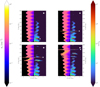 |
Fig. 1. Snapshots of the jet with an injected perturbation. The jet is propagating from the bottom to the top along the Z axis. The electron number density contour (in log-scale) is drawn on the left side, and the maximum value of the electron Lorentz factor (also in log-scale) on the right side. Both radial coordinates R and Z are given in Rjet units. The generated moving shock wave is located at ∼20 Rjet (A), ∼70 Rjet (B), ∼120 Rjet (C), and ∼170 Rjet (D) from the jet base and is marked with a white star. |
Our detection method successfully identifies the standing shock regions, where relativistic electrons are injected. In these zones, the fluid has a bulk Lorentz factor of γ = 3 and can accelerate in rarefaction regions up to γ = 4.
Map A in Fig. 1 shows the relativistic electron density and their maximum Lorentz factors of the jet shortly after injection of the perturbation. Since the strength of the shock waves decreases with distance from the jet inlet, the radial expansion of detected shock regions decreases with distance. Thus, electron injection takes place mainly at the first few shocks and the electrons undergo radiative cooling as they move away from the shocks.
Once the jet has reached its steady state, a perturbation is injected at its base as described above. Figures 1B and C show the propagation of the fast ejecta, which interacts strongly with the jet material and triggers a moving shock. This main moving shock goes through a weak deceleration phase each time it crosses a standing recollimation shock, which increases its thermal energy. A fraction of the jet material that is swept up and heated by the shock wave escapes radially toward the edge of the jet, which limits the amount of matter accreted by the moving shock and therefore its deceleration. As the moving shock runs into a rarefaction zone, it accelerates. This process is repeated each time the shock wave encounters a recollimation shock and its following rarefaction zone.
The first standing shock is only slightly disturbed by the passage of the moving shock. The second one is made to oscillate, leading to the emergence of rarefaction waves. In our setup, the third stationary shock is strongly destabilized. The interaction with the moving shock causes the emergence of a relaxation shock that propagates itself along the jet as a secondary moving, trailing shock.
As the primary moving shock sweeps up the jet material, it generates behind it a rarefaction zone (Figs. 1B and C). Initially, the rarefaction zone expands along the jet axis between the moving shock and the standing recollimation shock behind it. At the back of this zone, a relaxation shock emerges within the jet. During the first phase, until the moving shock reaches the third recollimation shock, the relaxation shock remains a compression wave. Afterward, this moving compression wave turns into a moving shock (Figs. 1B and C). Behind this relaxation shock, the recollimation shock undergoes a weak oscillation phase before it stabilizes. The strength of the relaxation shock increases with distance, disturbs the following recollimation shock more, and triggers another relaxation shock behind it. This succession of compression and rarefaction regions generated initially by the propagation of the perturbation is illustrated by the toy model in Fig. 2. At the end, when the moving shock and the trailing relaxation shocks leave the simulated jet, the jet recovers its quasi-initial state (Fig. 1D).
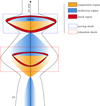 |
Fig. 2. Schematic representation of the jet geometry during the propagation of the primary perturbation. We represent the formation of a relaxation shock in the trail of the moving shock. The scheme is not to scale. |
4. Emission signature from moving and relaxation shocks
Applying the RIPTIDE post-processing code to the jet simulations, we calculated synthetic images and light curves for two observation angles (θobs = 20°, θobs = 90° from the jet axis) and for four frequencies (ν ∈ [1010, 1012, 1014, 1018] Hz), with a time step of Rjet/c. To investigate the impact of the LCE at θobs = 90°, we present results on a selected time range with a smaller time step of 0.05 Rjet/c in Appendix A.
4.1. Synthetic images
As seen in Fig. 1, which presents the jet in its initial, steady state, the shock strength decreases with distance from the jet inlet. Moreover, shocks are more pronounced toward the edge of the jet than along the jet axis, since the jet sound speed decreases outward. Consequently, more electrons are injected near the jet edges and they remain advected along the steady shock pattern. They cool down by synchrotron emission as they propagate away from the shocks. Therefore, X-ray emission is most pronounced at shocks close to the jet inlet (Fig. 3, bottom), where the highly relativistic electrons with γmax ≃ 107 cool promptly. In the radio band, electrons continue to emit as they are propagating along the jet, given the longer cooling time for smaller Lorentz factors (Fig. 3, top).
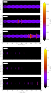 |
Fig. 3. Snapshots of the synchrotron emission maps of the jet before and after introduction of the ejecta, seen at two frequencies, ν = 1010 Hz (top) and ν = 1018 Hz (bottom). Each map represents the flux intensity in mJy units. The R and the Z axes are given in Rjet units. These maps represent the flux in the comoving frame for a viewing angle of θobs = 90° at three different comoving times (see the white boxes). The flux is evaluated at the distance of the radio galaxy 3C 111. |
The emission from the moving shocks (leading and trailing) follows the same behavior. Each time a moving shock interacts with a standing shock, the number of injected electrons grows, since ne = 0.01 ρ/mp. In the X-ray band, these electrons emit in a region close to the shock front and cool rapidly, while in the radio band,freshly injected electrons radiate during the propagation of the shock along the jet until they escape the jet at its edges. The escape time for the latter is close to Rjet/cℳ, the time taken by the moving shock to travel half the distance between two successive recollimation shocks.
In the synthetic maps, one also clearly sees the emergence of relaxation shocks after the third shock–shock interaction. If only one relaxation shock is visible at the beginning, their numbers increase at large distance. In the radio band, the emission surface associated with relaxation shocks increases and tends to dominate the emitted flux. In the X-ray band, individual relaxation shocks are clearly distinguishable.
4.2. Light curves
In Fig. 4 we present synthetic MWL light curves computed for a viewing angle of θobs = 90° and for four different frequencies (ν ∈ [1010, 1012, 1014, 1018] Hz). Overall a continuous increase in the total observed flux (in black) is seen until the main moving shock and trailing relaxation shocks leave the simulated jet. Each time a moving shock crosses a recollimation shock, a flare is triggered. This is particularly visible at high frequencies. As the LCE does not change the global shape of the light curve at θobs = 90° and with a time-step of Rjet/c, this effect is not taken into account here. Its impact on the detailed structure of the flares is shown in Fig. A.2, where a higher temporal resolution was used.
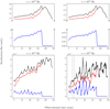 |
Fig. 4. Light curves obtained by integrating the total synchrotron flux. The computation of the light curve is realized for four different frequencies (see the titles). The overall flux is shown in black (upper curve), with the component from the original moving shock marked in blue (lowest curve) and the remaining jet emission in red. The flux is integrated from the injection time of the ejecta (at t = 0 yr) until t ∼ 250 yr. The dashed vertical lines in the plot with the X-ray light curve indicate the position of the first main flare (blue curve) and the associated flare echo from the perturbed jet (red curve). The flux is evaluated at the distance of the radio galaxy 3C 111. |
At radio frequencies ν = [1010, 1012] Hz, the flux is dominated by the emission from electrons injected on recollimation shocks (Fig. 4, red line) and propagating along the jet. Each time the leading moving shock interacts with a recollimation shock, a new electron population starts contributing to the total flux, which thus increases continuously. After each interaction, depending on its strength, the disturbed recollimation shock can radiate a remnant emission, which can lead to an elongation and asymmetry of the primary flare. The overall flux starts to decrease when the recollimation shocks relax to their initial states and when relaxations shocks leave the observed jet fraction.
With increasing frequency, from the optical (ν = 1014 Hz) to the X-ray band (ν = 1018 Hz), the proportion of the flux coming from the moving shock increases to reach on the average 20% of the total flux in our setup (Fig. 4, blue line). In the light curves, rapid variability can be seen for each interaction between the moving and standing shocks. In the X-ray band, the typical variability timescale is given by the size of the stationary emission region, for example 5−10 Rjet/c (in the comoving frame), as at this frequency the synchrotron cooling timescale is shorter. It corresponds to the radial advection of the electrons by the shocked jet fluid toward the ambient medium along the moving shock front (Meliani et al. 2007).
The proportion of the flux coming from standing shocks and relaxation shocks is still important at high frequencies. We observe, after each interaction, a radiative response of the jet, which can be classified in two types: during the two first shock–shock interactions, emission coming from perturbed standing shocks can be seen as delayed flares (or “flare echoes”; cf. Fig. 4, last panel, vertical lines). Starting from the third shock–shock interaction, delayed emission stemming from the moving relaxation shocks is added as well.
After the exit of the perturbation from the simulation box, relativistic electrons are still injected at moving relaxation shocks and provoke fast variability during interactions before the flux returns to its quasi-initial state (see Fig. 4). In Fig. 5 we represent a zoomed-in view of the light curves centered around the third standing shock. We clearly distinguish the flare and its associated echo and avoid being dominated by the large contribution from the emission of the surrounding jet.
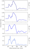 |
Fig. 5. Light curves for four different frequencies integrated between Z ∈ [75, 90] Rjet, for an observational time between t ∈ [4.8, 14.6] yr and a jet viewing angle of θobs = 90°. Fluxes are normalized to the maximum value. |
At X-ray frequencies, due to the fast cooling, the flares from electron injection into the moving shocks show a substructure of several peaks (see Fig. 5, bottom). As the standing shocks are formed by two shock fronts corresponding to the compression and rarefaction region (cf. Fig. 2), one observes two injection events for each passing of a moving shock. This structure is also visible in Fig. 4 (blue curve) in the X-ray light curve, for several flares coming from the principal moving shock. It should be noted that the width of the initial flare and flare echo in the radio band in Fig. 5 is artificially reduced by the restricted size of the zoomed-in simulation box. As seen in the full simulation, flares are wider in the radio band.
5. Discussion
5.1. Observable markers of jet relaxation
In our framework, we can classify the emission coming from the jet into four components. The first is the continuous emission from the steady jet, which corresponds to the more or less extensive emission coming from electrons injected at standing shocks. Second is the emission from the moving shock leading the ejecta, which causes strong variability at high frequencies due to fast-cooling electrons as the ejecta propagates through the jet. Third is the remnant emission coming from oscillating standing shocks following an interaction with the ejecta. Fourth is the emission from relaxation shocks trailing the leading shock. This emission can be extended over a long time.
The temporal evolution of the jet internal shocks structure at 90° and 20° in the presence of fast-moving ejecta is shown in Fig. 6, where the apparent distances from the base of the jet of the brightest regions in the radio emission maps are indicated as a function of time in the observer frame. The regular structure of the equally spaced standing shocks corresponds to the blue points. The leading moving shock (red points) is identified by a line of constant slope, corresponding to the apparent speed of the ejecta.
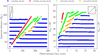 |
Fig. 6. Apparent distance traveled by standing and moving knots in time. Each point represents, for a given time, the position of local maxima in the radio synchrotron flux at ν = 1010 Hz. For θobs = 20°, the LCE is taken into account. The diagonal in the inset box corresponds to an apparent speed of c. |
In our simulations, the two first interactions with standing shocks cause remnant emissions that are clearly visible (especially in the X-ray band) in the light curves (see Fig. 4). At the third interaction, the resulting oscillation is sufficiently strong to lead to the emergence of a relaxation shock with a lower speed corresponding to a second diagonal line with a smaller slope in Fig. 6 (green points). The velocity of the relaxation shock is always greater than the jet velocity; an upper limit on the jet velocity can thus be determined by analyzing the velocity of such relaxation shocks. As can be seen in Fig. 6 for a viewing angle of 90°, the emergence of a relaxation shock at the intersection of a moving shock and a stationary shock is visible as a characteristic “fork” in the distance versus time plot. At 20°, this feature seems more difficult to detect (see the right part of Fig. 6), due to higher opacity in the radio band and the limiting spatial resolution.
Flare echoes may arise from the oscillation of perturbed standing shocks or from the propagation of relaxation shocks. This can be seen in Fig. 4 and more clearly in Fig. 5, where a first flare from the shock–shock interaction occurs after 60 years in the observer frame, followed by a second flare due to a relaxation wave 20 years later, for this specific event. In our simulations, a relaxation shock appears after the third interaction. From this point on, it is difficult to distinguish, in the light curve, the remnant emission from oscillating standing shocks and emission from relaxation shocks. A non-negligible emission counterpart due to either of the two mechanisms is expected at all frequencies and may be detected either as a separate flare echo or, if the initial flare has not ended by the time the secondary emission arises, in the form of a longer flare with a high asymmetry. The latter would be expected in particular in the radio band, where longer cooling times lead to a slower decay of the initial flare.
5.2. Observations of trailing shocks in 3C 111
Relaxation shocks may be identified with the trailing shocks that have already been detected in VLBI radio observations of several sources. Many of these trailing components do seem to appear after interactions of a moving radio knot with standing knots. Trailing components have apparent velocities that are always lower than that of the leading component.
A prominent example is the nearby Fanaroff-Riley II radio galaxy 3C 111, at a redshift of z = 0.049 (Truebenbach & Darling 2017). Its parsec-scale jet has been observed in the radio band (Kadler et al. 2008), in X-rays (Marscher 2006; Fedorova et al. 2020), and up to the γ-ray band (Grandi et al. 2012). Long-term VLBI monitoring of 3C 111 reveals the existence of bright superluminal knots (Preuss et al. 1988; Kadler et al. 2008; Schulz et al. 2020). Recent observations by Schulz et al. (2020), as well as Very Long Baseline Array (VLBA) polarization monitoring (Beuchert et al. 2018), suggest the presence of two stationary knots, C2 and C3, located respectively at ∼0.1 mas and 3 mas from the core.
During the period of 1996 to 1997, radio monitoring with the VLBA 2 cm Survey and the MOJAVE (Monitoring Of Jets in Active galactic nuclei with VLBA Experiments) monitoring programs detected two newly formed moving knots (named E and F; Kadler et al. 2008) emerging at the position where later on, during the 1999 observational campaign, the stationary knot C2 was detected (Beuchert et al. 2018). The appearance of knots E and F are associated with a bright radio flare event, which shows a strong asymmetry.
Additionally, in 2007 Schulz et al. (2020, Fig. 1) detected a second radio flare event with a complex flare structure. The authors suggest that trailing components are present and find some evidence of similarities between this event and the one in 1997, although the characteristic fork signature cannot be seen in this case. The radio flare seems correlated to the traveling of moving knots near the first recollimation shock, C2.
Kadler et al. (2008) interpreted the trailing component, F, as a reverse shock formed behind the leading knot, E, according to the scenario proposed by Perucho et al. (2008) using one-dimensional numerical hydrodynamic simulations. Further observations of the 1999 monitoring of the moving knot E show that at the position of the standing radio knot C3, the moving knot E splits up into a principal component E1 and three trailing components (E2, E3, and E4; Kadler et al. 2008). The emergence of these trailing features are interpreted by the authors following the scenario of the formation of conical moving shocks due to Kelvin-Helmholtz instabilities triggered solely by the propagation of an ejecta E within a hydrodynamic jet (Agudo et al. 2001). During this phase no noticeable flares were detected in association with the knots (E1, E2, E3, and E4).
5.3. Interpretation with the relaxation shock scenario
In our proposed scenario, we interpret the knot E as a leading moving shock formed by an ejecta and F as the first standing shock perturbed by the leading moving shock (Fig. 4). After the interaction, the standing shock relaxes and retrieves its initial position. We can understand the linear flux increase in component E (cf. Fig. 6 in Kadler et al. 2008) as a consequence of continuous injection of electrons at the moving shock. The fast decrease in the emission from knot F might be better explained by a remnant emission coming from a perturbed standing shock, than by a relaxation shock. Such displacements of perturbed standing shocks can be seen in Fig. 6 (orange points) with an apparent speed close to the speed of light. It should be noted that, for small viewing angles, such perturbed shocks are difficult to distinguish from relaxation shocks, due to strong Doppler boosting, combined with the LCE.
As the ejecta E is accelerated along the jet and interacts with C3, several trailing components, which we interpret as relaxation shocks, can be seen with a large variety of velocities. In our simulations, similar fork events can be seen at large distances from the core with an appearance of several relaxation shocks. The large number of relaxation shocks might be explained by the strength of the interaction of the main moving knot E with standing knot C3. The lower flux measured might be linked to a lower jet density in this region, as the moving shocks propagate in an expanding jet (Beuchert et al. 2018). Very recently, study by Weaver et al. (2022) updated the 43 GHz VLBA jet kinematic data for 3C 111 from the VLBA-BU-BLAZAR Program1. In their results, they may have find evidence of new trailing features which form the forked structure mention above.
The main difference between our scenario and the scenario proposed by Agudo et al. (2001) is the presence of stationary shocks in the jets. The presence of stationary components allows the emergence of relaxation shocks during their oscillation after a strong interaction. While their appearance is also possible in the absence of stationary components under certain conditions, interactions with such stationary components lead to a larger diversity of trailing components. Stationary components and their apparent drifting after interactions with a perturbation are observed in many sources with VLBI observations (Kim et al. 2020; Lico et al. 2022). The oscillation or drifting of stationary features can lead to additional emission counterparts and can help to explain observations as in the case of 3C 111.
5.4. Further examples for applications
Another example of where our scenario may apply is given by VLBI observations of the broad line radio galaxy 3C 120. Gomez et al. (2001) identified several trailing components triggered by an ejecta from the radio core in the 1998 VLBA data, which they ascribe to the result of dynamically induced recollimation shocks, again following Agudo et al. (2001). A later data set of VLBA monitoring data (Jorstad et al. 2017) then revealed three stationary knots at a distance of < 0.5 mas from the radio core (within the region where the trailing shocks arise). If these knots can be identified with stationary shocks that were already present, but undetected, in 1998, our scenario of relaxation shocks triggered by interactions between a primary moving shock and one or several standing shocks would apply.
More generally, observations of trailing components are not limited to prominent cases such as 3C 111 or 3C 120. Jorstad et al. (2005) have identified several sources with trailing components that may be signs of the presence of relaxation shocks. As an example, the radio sources PKS 0823+033 and 4C +10.45 show characteristic fork signatures of relaxation shocks (Appendix B).
In addition to the study of VLBI maps, relaxation shocks should also be detectable as flare echoes. As seen in Fig. 5, such temporal signatures are more easily distinguishable at high energies, such as in X-ray light curves. Compared to the radio band, flares are sharper at higher frequencies since self-absorption is negligible and the cooling timescales shorter in comparison with the dynamical time. X-ray flare echoes or flare asymmetries might provide evidence for relaxation shocks or remnant emission from perturbed standing shocks in blazars, where the small observation angles make the observation of fork events in VLBI very difficult. However, the identification of such events might be complicated by the impact of the LCE on the light curve.
6. Conclusion
We have investigated, for the first time, the emergence of relaxation shocks resulting from the interaction of strong moving and standing recollimation shocks in relativistic jets.
We carried out high resolution special-relativistic hydrodynamic simulations using the MPI-AMRVAC code of an over-pressured jet subject to a strong variability at its inlet. We developed a new radiative transfer code, RIPTIDE, which handles the LCE and is able to post-process large-scale high resolution special-relativistic hydrodynamic simulations of AGN jets for different observation angles and to compute synthetic synchrotron images and light curves at various frequencies.
Based on these simulations, we propose a scenario that is able to reproduce the formation and the propagation of transient trailing shocks observed in VLBI observations. In our scenario, such features are induced by the strong interaction between shocks inside the jet. We showed that during such interactions the standing shocks start to oscillate around their equilibrium position. For sufficiently strong oscillation events, new moving shocks are released, which follow the leading one.
The synthetic synchrotron light curves help us to distinguish between flares coming from interactions of the leading moving shock and additional flares associated with perturbed standing shocks and relaxation shocks. These additional components can lead to a high asymmetry of flares or flare echoes in the observed light curve.
A qualitative comparison of the expected observable features of the relaxation shock scenario with publicly available data of the radio galaxy 3C 111 seems promising. We propose a new coherent scenario to explain the appearance of different trailing components in VLBI observations and their emission counterpart in radio light curves. Trailing components are also seen in other radio galaxies, and this might again be explained with our scenario.
More informations at https://www.bu.edu/blazars/
Acknowledgments
The authors thank the anonymous reviewer for her or his peer review. Computations of the SR-HD results were carried out on the OCCIGEN cluster at CINES (https://www.cines.fr/) in Montpellier (project named lut6216, allocation A0090406842 and A0100412483). Radiative outputs given by the RIPTIDE code were carried out by the MesoPSL cluster at PSL University (http://www.mesopsl.fr/) in the Observatory of Paris. This work was granted access to the HPC resources of MesoPSL financed by the Region Ile de France and the project Equip at Meso (reference ANR-10-EQPX-29-01) of the programme Investissements dAvenir supervised by the Agence Nationale pour la Recherche. This research has made use of data from the MOJAVE database that is maintained by the MOJAVE team (Lister et al. 2018, 2021).
References
- Agudo, I., Gómez, J.-L., Martí, J.-M., et al. 2001, ApJ, 549, L183 [Google Scholar]
- Agudo, I., Gómez, J. L., Casadio, C., Cawthorne, T. V., & Roca-Sogorb, M. 2012, ApJ, 752, 92 [NASA ADS] [CrossRef] [Google Scholar]
- Aharonian, F. A., Barkov, M. V., & Khangulyan, D. 2017, ApJ, 841, 61 [NASA ADS] [CrossRef] [Google Scholar]
- Aleksi, J., Ansoldi, S., Antonelli, L. A., et al. 2014, Science, 346, 1080 [NASA ADS] [CrossRef] [Google Scholar]
- Beuchert, T., Kadler, M., Perucho, M., et al. 2018, A&A, 610, A32 [NASA ADS] [CrossRef] [EDP Sciences] [Google Scholar]
- Biretta, J. A., Junor, W., & Livio, M. 2002, New Astron. Rev., 46, 239 [Google Scholar]
- Blandford, R., Yuan, Y., Hoshino, M., & Sironi, L. 2017, Space Sci. Rev., 207, 291 [Google Scholar]
- Britzen, S., Kudryavtseva, N. A., Witzel, A., et al. 2010, A&A, 511, A57 [NASA ADS] [CrossRef] [EDP Sciences] [Google Scholar]
- Britzen, S., Fendt, C., Zajaček, M., et al. 2019, Galaxies, 7, 72 [NASA ADS] [CrossRef] [Google Scholar]
- Böttcher, M., & Baring, M. G. 2019, ApJ, 887, 133 [CrossRef] [Google Scholar]
- Čada, M., & Torrilhon, M. 2009, J. Comput. Phys., 228, 4118 [Google Scholar]
- Chiaberge, M., & Ghisellini, G. 1999, MNRAS, 306, 551 [Google Scholar]
- Fedorova, E., Hnatyk, B. I., Zhdanov, V. I., & Popolo, A. D. 2020, Universe, 6, 219 [NASA ADS] [CrossRef] [Google Scholar]
- Fichet de Clairfontaine, G., Meliani, Z., Zech, A., & Hervet, O. 2021, A&A, 647, A77 [NASA ADS] [CrossRef] [EDP Sciences] [Google Scholar]
- Fromm, C. M., Perucho, M., Ros, E., et al. 2011, A&A, 531, A95 [NASA ADS] [CrossRef] [EDP Sciences] [Google Scholar]
- Fromm, C. M., Ros, E., Perucho, M., et al. 2013a, A&A, 551, A32 [NASA ADS] [CrossRef] [EDP Sciences] [Google Scholar]
- Fromm, C. M., Ros, E., Perucho, M., et al. 2013b, A&A, 557, A105 [NASA ADS] [CrossRef] [EDP Sciences] [Google Scholar]
- Fromm, C. M., Perucho, M., Mimica, P., & Ros, E. 2016, A&A, 588, A101 [NASA ADS] [CrossRef] [EDP Sciences] [Google Scholar]
- Ghisellini, G., Tavecchio, F., Maraschi, L., Celotti, A., & Sbarrato, T. 2014, Nature, 515, 376 [NASA ADS] [CrossRef] [Google Scholar]
- Gomez, J.-L., Marscher, A. P., Alberdi, A., Jorstad, S. G., & Agudo, I. 2001, ApJ, 561, L161 [NASA ADS] [CrossRef] [Google Scholar]
- Gómez, J. L., Martí, J. M., Marscher, A. P., Ibáñez, J. M., & Alberdi, A. 1997, ApJ, 482, L33 [Google Scholar]
- Grandi, P., Torresi, E., & Stanghellini, C. 2012, ApJ, 751, L3 [NASA ADS] [CrossRef] [Google Scholar]
- Hervet, O., Boisson, C., & Sol, H. 2016, A&A, 592, A22 [NASA ADS] [CrossRef] [EDP Sciences] [Google Scholar]
- Hervet, O., Meliani, Z., Zech, A., et al. 2017, A&A, 606, A103 [NASA ADS] [CrossRef] [EDP Sciences] [Google Scholar]
- Huber, D., Kissmann, R., Reimer, A., & Reimer, O. 2021, A&A, 646, A91 [NASA ADS] [CrossRef] [EDP Sciences] [Google Scholar]
- Jorstad, S. G., Marscher, A. P., Lister, M. L., et al. 2005, AJ, 130, 1418 [Google Scholar]
- Jorstad, S. G., Marscher, A. P., Smith, P. S., et al. 2013, ApJ, 773, 147 [Google Scholar]
- Jorstad, S. G., Marscher, A. P., Morozova, D. A., et al. 2017, ApJ, 846, 98 [Google Scholar]
- Kadler, M., Ros, E., Perucho, M., et al. 2008, ApJ, 680, 867 [NASA ADS] [CrossRef] [Google Scholar]
- Keppens, R., Meliani, Z., van Marle, A. J., et al. 2012, J. Comput. Phys., 231, 718 [Google Scholar]
- Keppens, R., Teunissen, J., Xia, C., & Porth, O. 2020, Comput. Math. Appl., submitted [arXiv:2004.03275] [Google Scholar]
- Kim, D.-W., Trippe, S., & Kravchenko, E. V. 2020, A&A, 636, A62 [EDP Sciences] [Google Scholar]
- Lico, R., Casadio, C., Jorstad, S. G., et al. 2022, A&A, 658, L10 [NASA ADS] [CrossRef] [EDP Sciences] [Google Scholar]
- Lister, M. L., Aller, H. D., Aller, M. F., et al. 2009, AJ, 137, 3718 [Google Scholar]
- Lister, M. L., Aller, M. F., Aller, H. D., et al. 2013, AJ, 146, 120 [Google Scholar]
- Lister, M. L., Aller, M. F., Aller, H. D., et al. 2018, ApJS, 234, 12 [CrossRef] [Google Scholar]
- Lister, M. L., Homan, D. C., Kellermann, K. I., et al. 2021, ApJ, 923, 30 [NASA ADS] [CrossRef] [Google Scholar]
- Marscher, A. P. 2006, Astron. Nachr., 327, 217 [NASA ADS] [CrossRef] [Google Scholar]
- Marscher, A. P., & Gear, W. K. 1985, ApJ, 298, 114 [Google Scholar]
- Marscher, A. P., Jorstad, S. G., D’Arcangelo, F. D., et al. 2008, Nature, 452, 966 [Google Scholar]
- Marshall, H. L., Miller, B. P., Davis, D. S., et al. 2002, ApJ, 564, 683 [Google Scholar]
- Massaro, E., Perri, M., Giommi, P., & Nesci, R. 2004, A&A, 413, 489 [NASA ADS] [CrossRef] [EDP Sciences] [Google Scholar]
- Mathews, W. G. 1971, ApJ, 165, 147 [Google Scholar]
- Meliani, Z., & Keppens, R. 2007, A&A, 475, 785 [NASA ADS] [CrossRef] [EDP Sciences] [Google Scholar]
- Meliani, Z., Sauty, C., Tsinganos, K., & Vlahakis, N. 2004, A&A, 425, 773 [NASA ADS] [CrossRef] [EDP Sciences] [Google Scholar]
- Meliani, Z., Keppens, R., Casse, F., & Giannios, D. 2007, MNRAS, 376, 1189 [NASA ADS] [CrossRef] [Google Scholar]
- Mignone, A., & Bodo, G. 2006, MNRAS, 368, 1040 [Google Scholar]
- Mimica, P., Aloy, M. A., Agudo, I., et al. 2009, ApJ, 696, 1142 [Google Scholar]
- Nieppola, E., Hovatta, T., Tornikoski, M., et al. 2009, ApJ, 137, 5022 [CrossRef] [Google Scholar]
- Pelletier, G., Gremillet, L., Vanthieghem, A., & Lemoine, M. 2019, Phys. Rev. E, 100, 013205 [Google Scholar]
- Perlman, E. S., Biretta, J. A., Zhou, F., Sparks, W. B., & Macchetto, F. D. 1999, AJ, 117, 2185 [NASA ADS] [CrossRef] [Google Scholar]
- Perucho, M., Agudo, I., Gómez, J. L., et al. 2008, A&A, 489, L29 [NASA ADS] [CrossRef] [EDP Sciences] [Google Scholar]
- Plotnikov, I., Grassi, A., & Grech, M. 2018, MNRAS, 477, 5238 [Google Scholar]
- Preuss, E., Alef, W., & Kellermann, K. I. 1988, in The Impact of VLBI on Astrophysics and Geophysics, eds. M. J. Reid, & J. M. Moran, 129, 105 [NASA ADS] [CrossRef] [Google Scholar]
- Pushkarev, A. B., Kovalev, Y. Y., Lister, M. L., & Savolainen, T. 2017, MNRAS, 468, 4992 [Google Scholar]
- Raiteri, C. M., Villata, M., Acosta-Pulido, J. A., et al. 2017, Nature, 552, 374 [NASA ADS] [CrossRef] [Google Scholar]
- Schulz, R., Kadler, M., Ros, E., et al. 2020, A&A, 644, A85 [NASA ADS] [CrossRef] [EDP Sciences] [Google Scholar]
- Shukla, A., & Mannheim, K. 2020, Nat. Commun., 11, 4176 [NASA ADS] [CrossRef] [Google Scholar]
- Stawarz, Ł., Aharonian, F., Kataoka, J., et al. 2006, MNRAS, 370, 981 [NASA ADS] [CrossRef] [Google Scholar]
- Tammi, J., & Duffy, P. 2009, MNRAS, 393, 1063 [NASA ADS] [CrossRef] [Google Scholar]
- Tramacere, A., Massaro, E., & Taylor, A. M. 2011, ApJ, 739, 66 [Google Scholar]
- Truebenbach, A. E., & Darling, J. 2017, ApJS, 233, 3 [CrossRef] [Google Scholar]
- Vaidya, B., Mignone, A., Bodo, G., Rossi, P., & Massaglia, S. 2018, ApJ, 865, 144 [Google Scholar]
- van Eerten, H. J., Leventis, K., Meliani, Z., Wijers, R. A. M. J., & Keppens, R. 2010, MNRAS, 403, 300 [NASA ADS] [CrossRef] [Google Scholar]
- Vlasis, A., van Eerten, H. J., Meliani, Z., & Keppens, R. 2011, MNRAS, 415, 279 [NASA ADS] [CrossRef] [Google Scholar]
- Walker, R. C., Hardee, P. E., Davies, F. B., Ly, C., & Junor, W. 2018, ApJ, 855, 128 [Google Scholar]
- Weaver, Z. R., Jorstad, S. G., Marscher, A. P., et al. 2022, ApJS, submitted [arXiv:2202.12290] [Google Scholar]
- Wehrle, A. E., Grupe, D., Jorstad, S. G., et al. 2016, ApJ, 816, 53 [Google Scholar]
- Wilson, M. J. 1987, MNRAS, 226, 447 [NASA ADS] [CrossRef] [Google Scholar]
- Wilson, A. S., & Yang, Y. 2002, ApJ, 568, 133 [Google Scholar]
- Winner, G., Pfrommer, C., Girichidis, P., & Pakmor, R. 2019, MNRAS, 488, 2235 [Google Scholar]
- Zanotti, O., Rezzolla, L., Del Zanna, L., & Palenzuela, C. 2010, A&A, 523, A8 [NASA ADS] [CrossRef] [EDP Sciences] [Google Scholar]
- Zhang, W., & MacFadyen, A. 2009, ApJ, 698, 1261 [NASA ADS] [CrossRef] [Google Scholar]
Appendix A: Light crossing effect
A.1. Implementation and test on a toy model
The method we implemented to account for the LCE is an extension of the procedure described by Chiaberge & Ghisellini (1999), which was limited to a simple geometry of the emission region, seen by a comoving observer under an angle of 90°.
The implementation of the LCE requires knowledge of the simulation time step Δt′ and average bulk Doppler factor of the jet. Depending on these parameters, we divide the simulation box, projected in the observer’s frame for a given viewing angle, into N layers perpendicularly to the observer’s l.o.s., such that the width of each layer equals the distance light travels in one time step in the observer frame Δtobs (cf. Eq. 13).
We first tested the procedure on a simple toy model, similar to the one referred to by Chiaberge & Ghisellini (1999), which describes a flare event where a moving shock crosses a standing shock. The two-dimensional jet is modeled with square cells and the standing shock region corresponds to a small slice of a few cell columns (red region in Fig. A.1). The interaction is represented by the injection of electrons in all cells inside the shock region. As the moving shock passes through the standing shock region, injection takes place first at the beginning of the region at time tstart and then also in consecutive columns. Injection stops everywhere, as the moving shock exits from the region at time tend. The post-processing code is directly applied to this model, assuming a viewing angle of 90° in the observer frame. As electrons are injected in the cells moving through the shock region, a flare appears in the synthetic synchrotron light curve.
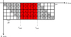 |
Fig. A.1. Schematic representation of our toy model. The red area represents the region where the shock is “on”, gray when it is “off”. The number on each cell indicates the generation of electrons. |
In Fig. A.1, the numbers correspond to time steps in the observer frame. Light from cells with the same number reaches the observer at the same time. At time step 1, the observer starts detecting emission from the onset of the shock interaction, but only from a position at the front edge of the jet and at the beginning of the shock region. For consecutive time steps, emission reaches the observer from cells farther along the jet, as the moving shock crosses the standing shock region. At the same time, emission from cells closer to the jet axis has propagated to the observer through the jet. This leads to the diagonal arrangement of cells with the same number. After the shock has left the standing shock region, emission will continue during time steps 6, 7, 8, 9, as photons close to the jet axis arrive at the observer with an additional delay of Δtobs = c ⋅ l for each additional time step, where l is the width of one cell.
To correctly account for this effect, before treating the ray tracing along each vertical column, the jet is split into layers, corresponding to the rows of cells in the toy model example. Each consecutive layer is shifted by one additional time step, such that, for example, photons emitted from the second layer propagate into the front layer, as it appears one time step later.
The resulting effect for the toy model is seen in Fig. A.2. Ignoring the LCE, the light curve is a simple Heaviside function with a width corresponding to the size of the injection region (red curve). Turning on the LCE, the number of “activated” cells for a given time step follows a moving average with a maximum at time step 5, when injection occurs over the whole stationary shock region. The result with a full treatment of the LCE is shown as the dashed blue curve. The change in shape is in good agreement with the result from Chiaberge & Ghisellini (1999) at high energies (see Fig. 6 in their paper).
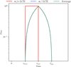 |
Fig. A.2. Light curves (ν = 1018 Hz) with and without the LCE obtained for an observed situated in the co-mobile frame at θobs = 90°. |
For this particular case of a simple geometric emission region and a 90° observation angle, one can reproduce the LCE by applying a simple moving average on the light curve, as is shown with the green curve, requiring far less computing time. The temporal width of this moving average must be equal to the light crossing time of one layer.
A.2. Application to full simulations for various θobs
We first apply the “layer method” to full jet simulations for a viewing angle of θobs = 90° in the observer frame. The simulation time step needs to be sufficiently small, compared to the light crossing time of the jet radius, if one wants to resolve the LCE. Here we present results with  (while for the general simulation we are using 1 Rjet/c). Due to the large amount of computing time, we restricted the ray tracing treatment to emission coming from a restrained area of the jet centered on an X-ray flare event. At this angle, the LCE leads only to a small distortion and smoothing of the overall shape of the light curve, without a significant impact on the observable structure.
When comparing the result with an application of a simple moving average (cf. A.1), a good agreement is seen. The residuals between both methods show an average relative error of ∼1%.
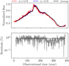 |
Fig. A.3. Light curves with (blue) and without (red) the LCE for 1018 Hz at θobs = 90°. The dark line represents the “moving average method”. The gray line in the lower panel shows the residuals between both methods (light curves with the LCE minus the moving average over the light curve with the LCE). |
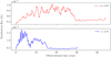 |
Fig. A.4. Light curve without and with the LCE for 1018 Hz at θobs = 20°. The flux is evaluated at the distance of the radio galaxy 3C 111. |
We also present a result with a much smaller observation angle of θobs = 20°, using the nominal simulation time step of Rjet/c. We here compute the light curve by integrating the flux over the entire simulated jet, focusing again on the X-ray band. At this angle, the LCE has a significant impact on the observed light curve. We recover a temporal compression of the light curve, with flare activities concentrated in a period of ∼5 yr. This shortened timescale is also reflected in Fig. 6. Due to the apparent superluminal motion, the flare variability decreases to reach 150−200 days. Additionally, the shape of the flares changes but dedicated, computationally intensive simulations with smaller time steps are needed for a more detailed study, which is beyond the scope of this work.
Appendix B: Two further sources with potential trailing shocks
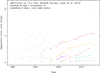 |
Fig. B.1. Core separation versus time for the source PKS 0823+033. Components 8 and 13 are candidates for relaxation shocks. A stationary shock is labeled “12”. |
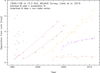 |
Fig. B.2. Core separation versus time for the source 4C +10.45. Component 8 may be a potential relaxation shock with component 9 as a stationary shock. |
In this section we present two further radio galaxies showing signs of the presence of trailing components in the core separation versus time plot, in the form of “fork events” connected to stationary knots. We use the MOJAVE database maintained by the MOJAVE team (Lister et al. 2018, 2021).
All Tables
All Figures
|
Fig. 1. Snapshots of the jet with an injected perturbation. The jet is propagating from the bottom to the top along the Z axis. The electron number density contour (in log-scale) is drawn on the left side, and the maximum value of the electron Lorentz factor (also in log-scale) on the right side. Both radial coordinates R and Z are given in Rjet units. The generated moving shock wave is located at ∼20 Rjet (A), ∼70 Rjet (B), ∼120 Rjet (C), and ∼170 Rjet (D) from the jet base and is marked with a white star. |
| In the text | |
|
Fig. 2. Schematic representation of the jet geometry during the propagation of the primary perturbation. We represent the formation of a relaxation shock in the trail of the moving shock. The scheme is not to scale. |
| In the text | |
|
Fig. 3. Snapshots of the synchrotron emission maps of the jet before and after introduction of the ejecta, seen at two frequencies, ν = 1010 Hz (top) and ν = 1018 Hz (bottom). Each map represents the flux intensity in mJy units. The R and the Z axes are given in Rjet units. These maps represent the flux in the comoving frame for a viewing angle of θobs = 90° at three different comoving times (see the white boxes). The flux is evaluated at the distance of the radio galaxy 3C 111. |
| In the text | |
|
Fig. 4. Light curves obtained by integrating the total synchrotron flux. The computation of the light curve is realized for four different frequencies (see the titles). The overall flux is shown in black (upper curve), with the component from the original moving shock marked in blue (lowest curve) and the remaining jet emission in red. The flux is integrated from the injection time of the ejecta (at t = 0 yr) until t ∼ 250 yr. The dashed vertical lines in the plot with the X-ray light curve indicate the position of the first main flare (blue curve) and the associated flare echo from the perturbed jet (red curve). The flux is evaluated at the distance of the radio galaxy 3C 111. |
| In the text | |
|
Fig. 5. Light curves for four different frequencies integrated between Z ∈ [75, 90] Rjet, for an observational time between t ∈ [4.8, 14.6] yr and a jet viewing angle of θobs = 90°. Fluxes are normalized to the maximum value. |
| In the text | |
|
Fig. 6. Apparent distance traveled by standing and moving knots in time. Each point represents, for a given time, the position of local maxima in the radio synchrotron flux at ν = 1010 Hz. For θobs = 20°, the LCE is taken into account. The diagonal in the inset box corresponds to an apparent speed of c. |
| In the text | |
|
Fig. A.1. Schematic representation of our toy model. The red area represents the region where the shock is “on”, gray when it is “off”. The number on each cell indicates the generation of electrons. |
| In the text | |
|
Fig. A.2. Light curves (ν = 1018 Hz) with and without the LCE obtained for an observed situated in the co-mobile frame at θobs = 90°. |
| In the text | |
|
Fig. A.3. Light curves with (blue) and without (red) the LCE for 1018 Hz at θobs = 90°. The dark line represents the “moving average method”. The gray line in the lower panel shows the residuals between both methods (light curves with the LCE minus the moving average over the light curve with the LCE). |
| In the text | |
|
Fig. A.4. Light curve without and with the LCE for 1018 Hz at θobs = 20°. The flux is evaluated at the distance of the radio galaxy 3C 111. |
| In the text | |
|
Fig. B.1. Core separation versus time for the source PKS 0823+033. Components 8 and 13 are candidates for relaxation shocks. A stationary shock is labeled “12”. |
| In the text | |
|
Fig. B.2. Core separation versus time for the source 4C +10.45. Component 8 may be a potential relaxation shock with component 9 as a stationary shock. |
| In the text | |
Current usage metrics show cumulative count of Article Views (full-text article views including HTML views, PDF and ePub downloads, according to the available data) and Abstracts Views on Vision4Press platform.
Data correspond to usage on the plateform after 2015. The current usage metrics is available 48-96 hours after online publication and is updated daily on week days.
Initial download of the metrics may take a while.